Density matrix Monte Carlo modeling of quantum cascade lasers

Abstract

By including elements of the density matrix formalism, the semiclassical ensemble Monte Carlo method for carrier transport is extended to incorporate incoherent tunneling, known to play an important role in quantum cascade lasers (QCLs). In particular, this effect dominates electron transport across thick injection barriers, which are frequently used in terahertz QCL designs. A self-consistent model for quantum mechanical dephasing is implemented, eliminating the need for empirical simulation parameters. Our modeling approach is validated against available experimental data for different types of terahertz QCL designs.

I Introduction

Advanced carrier transport modeling techniques for semiconductor devices evaluate the relevant processes, such as different scattering mechanisms, directly based on the corresponding Hamiltonians. Consequently, these approaches do not require specific experimental or empirical input, but only rely on well known material parameters. Especially for the modeling of advanced semiconductor nanodevices, theoretical methods beyond the standard drift-diffusion model are required. Various theoretical approaches with different levels of complexity are available, such as the ensemble Monte Carlo (EMC) method Jacoboni and Lugli (1989) or the nonequilibrium Green’s function (NEGF) approach Schwinger (1961); Kadanoff and Baym (1962); Keldysh (1965); Jirauschek and Kubis (2014).

Here, we focus on the modeling of quantum cascade lasers (QCLs) Faist et al. (1994). These devices are highly interesting from a scientific point of view as well as with respect to various applications, e.g., in metrology and sensing, and are already commercially available Curl et al. (2010). The active region consists of a quantum well structure, where the laser levels are formed between the quantized electron states in the conduction band. Thus, the lasing wavelength does not primarily depend on the material system used, but can be selected over a wide spectral range by adequate quantum design. In particular, the mid-infrared and terahertz (THz) regions become accessible, thus complementing the spectral range covered by conventional semiconductor lasers.

Modeling provides detailed insight into the complex interplay of the physical effects involved and allows for a systematic optimization of QCL designs, e.g., with respect to efficiency, operating temperature and spectral range. The ideal simulation approach should offer excellent accuracy and versatility, combined with decent computational efficiency to allow for design optimization over an extended parameter range. Advanced carrier transport modeling techniques not only consider the quantized energy states due to the electron confinement in growth direction, but also the in-plane wavevectors which are related to the kinetic electron energies. In this way, both the inter- and intrasubband carrier dynamics can be considered. EMC has been widely employed for the analysis and design of QCLs, offering a good compromise between reliability and numerical effort Borowik et al. (2017); Iotti and Rossi (2000); Köhler et al. (2001); Callebaut et al. (2003, 2004); Compagnone et al. (2002); Lü and Cao (2006a); Gao et al. (2007a, b); Mátyás et al. (2010, 2011); Jirauschek and Lugli (2009); Bonno et al. (2005). However, as a semiclassical method EMC neglects quantum coherence effects, most notably tunnel coupling between the two states spanning the injection barriers and the level broadening of the states Weber et al. (2009). Such effects become relevant especially for thick barriers, where the states involved in the electron transport have a small energy separation, and the electron transport is governed by resonant tunneling. This applies especially to the injection barriers in various types of THz QCL designs Callebaut and Hu (2005); Weber et al. (2009). Consequently, also quantum transport approaches are frequently used for the simulation of QCLs, including NEGF Wacker (2002); Banit et al. (2005); Kubis et al. (2009); Schmielau and Pereira (2009); Kubis and Vogl (2011); Schmielau and Pereira (2009); Kolek et al. (2012); Winge et al. (2012); Wacker et al. (2013); Grange (2015) as well as the density matrix (DM) Iotti and Rossi (2001a); Weber et al. (2009); Iotti and Rossi (2016); Lindskog et al. (2014) and related Wigner function Jonasson and Knezevic (2015) formalism. The computational load of these approaches is much higher than for their semiclassical counterparts, impeding their applicability to complex QCL structures with many subbands, and to QCL design and optimization in general.

Various strategies exist to obtain a simulation approach which includes the most important quantum effects and still provides acceptable computational efficiency. Particularly for the DM approach, the in-plane wavevector dependence is frequently neglected, reducing the order of the density matrix to the number of considered subbands Kumar and Hu (2009); Dupont et al. (2010); Terazzi and Faist (2010); Dinh et al. (2012); Fathololoumi et al. (2012). Another approach is to reduce the numerical burden of full quantum transport simulation methods by introducing simplifications. In particular, for NEGF various approximations have been developed which greatly simplify the evaluation of the scattering self-energies. This includes the constant $k$ approximation which assumes that the scattering self-energies are independent of the in-plane wavevector Schmielau and Pereira (2009); Kubis and Vogl (2011); Wacker et al. (2013), and the multi-scattering Büttiker probe model where the lesser self-energies are replaced by a quasi-equilibrium expression Greck et al. (2015). An opposite strategy is to start with a semiclassical method such as EMC and extend it to include quantum effects relevant for the carrier transport. An example is the consideration of collisional broadening in EMC Aksamija and Ravaioli (2009); Matyas et al. (2013). Furthermore, the DM formalism has been combined with EMC to describe the incoherent tunneling transport across thick injection barriers Callebaut and Hu (2005); Bhattacharya et al. (2012); Freeman (2016); Freeman and Karunasiri (2012). This hybrid approach overcomes the main weakness of semiclassical transport simulations, which treat the carrier transport through a barrier as instantaneous since electrons scattered into states extending over the barrier see no resistance Callebaut and Hu (2005). For biases where narrow anticrossings occur, this can result in excessive current spikes, indicating the breakdown of the semiclassical description Mátyás et al. (2010).

In this paper, we extend EMC to include incoherent tunneling transport, building upon the pioneering work of Callebaut and Hu Callebaut and Hu (2005). As in previous related approaches Callebaut and Hu (2005); Bhattacharya et al. (2012); Freeman (2016); Freeman and Karunasiri (2012), we use localized basis states to describe the incoherent tunneling mechanism. However, here this effect is not considered by solving the von Neumann and the Boltzmann transport equations in parallel, but rather directly built into EMC as an additional ”scattering-like” mechanism derived from the DM formalism. This enables a straightforward implementation into existing EMC codes, without significantly increasing the numerical load. In this way, all the features of advanced EMC QCL simulation tools, such as the consideration of electron-electron scattering beyond the Hartree approximation and coupling between carrier transport and optical cavity field Goodnick and Lugli (1988); Jirauschek (2010); Jirauschek and Kubis (2014), are taken advantage of. Furthermore, in the resulting DM-EMC approach the self-consistent character of EMC is preserved by implementing a self-consistent model for the dephasing rate Unuma et al. (2003); Freeman (2016); Ando (1985), thus avoiding the need for empirical parameters.

II Method

II.1 Localized states and tunneling

Electron transport across thick barriers, such as the injection barriers in various types of THz QCL designs, is governed by incoherent tunneling between near-resonant states Callebaut and Hu (2005); Weber et al. (2009). For these, the use of localized wavefunctions has proven advantageous, as can be obtained from a tight binding approach Callebaut and Hu (2005); Bhattacharya et al. (2012); Freeman (2016); Freeman and Karunasiri (2012). Rather than determining the extended eigenstates for the actual potential $V$ as in semiclassical simulations [see Fig. 1(a)], the active region structure is divided into modules separated by thick barriers, where each module is described by a separate potential $V_{\mathrm{tb}}$, as indicated in Fig. 1(b). The wavefunctions and eigenenergies are then calculated for each module separately using a Schrödinger-Poisson solver. In this tight-binding framework, the transport within a module can be implemented into EMC in the usual way by evaluating scattering-induced transport, since quantum coherence effects only appear for transitions across the module boundaries. We note that this approach can straightforwardly be extended to structures containing more than one thick barrier per period Dupont et al. (2010).

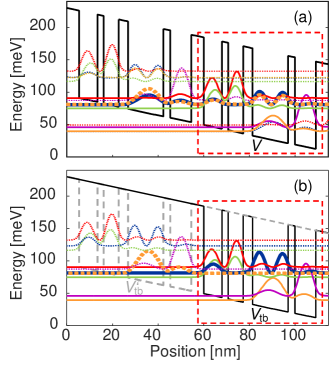
Figure 1: Conduction band profile and probability densities for a four-well THz QCL Benz et al. (2007) at a bias of $7.6\,\mathrm{kV}/\mathrm{cm}$, computed based on (a) the actual potential $V$ and (b) the tight-binding potential $V_{\mathrm{tb}}$. The rectangles denote a single QCL period. The wavefunctions involved in the electron transport across the thick barrier are marked by bold lines.

In our model, an electron state $\left|i,\mathbf{k}\right\rangle$ is characterized by its subband energy $E_{i}$, tight-binding wavefunction $\psi_{i}\left(z\right)$ where $z$ denotes the position coordinate along the growth direction, and in-plane wavevector $\mathbf{k}$. In the following, we assume decoupling between the confinement in $z$ direction and in-plane motion which strictly holds for infinite quantum wells Ekenberg (1989), implying $\mathbf{k}$ independent wavefunctions $\psi_{i}\left(z\right)$. The decoupling approximation also works reasonably well for finite, not too narrow quantum wells, and is frequently used for QCL modeling to reduce complexity Savić et al. (2006). Furthermore, decoupling is maintained for an elementary treatment of nonparabolicity, where an energy dependent effective mass is used to determine the $\psi_{i}\left(z\right)$ and $E_{i}$, and subsequently, for each subband $i$ an effective mass $m_{i}^{\ast}$ is computed describing the electron dispersion relation at the corresponding subband bottom Ekenberg (1989); Jirauschek and Kubis (2014).

Tunneling from a state $\left|i,\mathbf{k}\right\rangle$ to states $\left|j,\mathbf{k}\right\rangle$ across a barrier can be described by a density matrix equation combined with rate equation terms Iotti and Rossi (2001a); Terazzi and Faist (2010),

$$\mathrm{d}_{t}\rho_{ii,\mathbf{k}} =\sum_{\left(j,\mathbf{k}^{\prime}\right)\neq\left(i,\mathbf{k}\right)}r_{j,\mathbf{k}^{\prime}\rightarrow i,\mathbf{k}}\rho_{jj,\mathbf{k}^{\prime}}-r_{i,\mathbf{k}}\rho_{ii,\mathbf{k}}$$

$$+\sum_{j}\mathrm{i}\Omega_{ij}\left(\rho_{ij,\mathbf{k}}-\rho_{ji,\mathbf{k}}\right),$$ (1a)

$$\mathrm{d}_{t}\rho_{ij,\mathbf{k}} =\sum_{n}\mathrm{i}\left(\Omega_{nj}\rho_{in,\mathbf{k}}-\Omega_{in}\rho_{nj,\mathbf{k}}\right)-\mathrm{i}\omega_{ij}\rho_{ij,\mathbf{k}}-\gamma_{ij,\mathbf{k}}\rho_{ij,\mathbf{k}}.$$ (1b)

The diagonal density matrix elements $$\rho_{ii,\mathbf{k}} \left|i,\mathbf{k}\right\rangle \rho_{ij,\mathbf{k}} \left|i,\mathbf{k}\right\rangle \left|j,\mathbf{k}\right\rangle r_{j,\mathbf{k}^{\prime}\rightarrow i,\mathbf{k}} \left|j,\mathbf{k}^{\prime}\right\rangle \left|i,\mathbf{k}\right\rangle r_{i,\mathbf{k}} \left|i,\mathbf{k}\right\rangle$$ correspond to the electron occupation of state , while the off-diagonal elements are related to the coherences between states  and . The scattering rates from all possible states  to correspond in our approach to the conventional EMC scattering rates, and is the total scattering rate from state into all other states,

$$r_{i,\mathbf{k}}=\sum_{\left(j,\mathbf{k}^{\prime}\right)\neq\left(i,\mathbf{k}\right)}r_{i,\mathbf{k}\rightarrow j,\mathbf{k}^{\prime}}.$$ (2)

The modeling of the dephasing rate $\gamma_{ij,\mathbf{k}}$ is discussed in Section II.2. Furthermore, $\omega_{ij}=\left(E_{i}-E_{j}\right)/\hbar$ denotes the resonance frequency between states $\left|i,\mathbf{k}\right\rangle$ and $\left|j,\mathbf{k}\right\rangle$, which is $\mathbf{k}$ independent for parabolic subbands with identical effective mass. With the extended and tight-binding potentials $V$ and $V_{\mathrm{tb}}$ illustrated in Figs. 1(a) and 1(b), respectively, the tunnel coupling is approximately described by the matrix element $\left\langle i,\mathbf{k}\right|V-V_{\mathrm{tb}}\left|j,\mathbf{k}^{\prime}\right\rangle$. This expression becomes $0$ for $\mathbf{k}\neq\mathbf{k}^{\prime}$ since $V$ and $V_{\mathrm{tb}}$ only depend on $z$, and is given by $\hbar\Omega_{ij}$ for $\mathbf{k}=\mathbf{k}^{\prime}$, with the Rabi frequency $\Omega_{ij}=\left\langle\psi_{i}\right|V-V_{\mathrm{tb}}\left|\psi_{j}\right\rangle/\hbar$. Thus, in our model given by Eq. (1), incoherent tunneling only occurs between states with identical $\mathbf{k}$ Iotti and Rossi (2001a); Callebaut and Hu (2005); Wacker (2001, 2002). Furthermore, since in our approach this effect is only considered across thick barriers separating the individual modules, $\Omega_{ij}$ is nonzero only for the state doublets spanning these barriers Terazzi and Faist (2010).

In the following, interference effects between different tunneling transitions involving the same subband $i$ to the left or $j$ to the right of the barrier are neglected, i.e., only the terms containing $\Omega_{ij}$ are kept in the sum of Eq. (1b) Razavipour et al. (2013). The stationary solution of Eq. (1) is obtained by setting $\mathrm{d}_{t}=0$, which yields

$$0 =\sum_{\left(j,\mathbf{k}^{\prime}\right)\neq\left(i,\mathbf{k}\right)}r_{j,\mathbf{k}^{\prime}\rightarrow i,\mathbf{k}}\rho_{jj,\mathbf{k}^{\prime}}-r_{i,\mathbf{k}}\rho_{ii,\mathbf{k}}$$

$$+\sum_{j}\left(\rho_{jj,\mathbf{k}}-\rho_{ii,\mathbf{k}}\right)r_{i\rightarrow j,\mathbf{k}}^{\mathrm{t}},$$ (3)

with the single-electron tunneling rate from $\left|i,\mathbf{k}\right\rangle$ to $\left|j,\mathbf{k}\right\rangle$ given by

$$r_{i\rightarrow j,\mathbf{k}}^{\mathrm{t}}=\frac{2\Omega_{ij}^{2}\gamma_{ij,\mathbf{k}}}{\omega_{ij}^{2}+\gamma_{ij,\mathbf{k}}^{2}}.$$ (4)

Equation (3) is compatible with the EMC framework, since the tunneling rate given in Eq. (4) can be straightforwardly implemented as a pseudo-scattering mechanism. For calculating $\Omega_{ij}$, we consider the asymmetry of the structure with respect to the tunneling barrier, introduced by the module design and the applied bias, by using the improved formula $\left(\hbar\Omega_{ij}\right)^{2}=\left\langle\psi_{i}\right|V-V_{\mathrm{tb}}\left|\psi_{j}\right\rangle\left\langle\psi_{i}\right|V-V_{\mathrm{tb}}^{\prime}\left|\psi_{j}\right\rangle$. Here, $V_{\mathrm{tb}}^{\prime}$ and $V_{\mathrm{tb}}$ are the tight-binding potentials of the modules to the left and right of the tunneling barrier, respectively [see Fig. 1(b)] Grier et al. (2015); Yariv et al. (1985). Pauli blocking is accounted for by considering the final state occupation probability $f_{j,\mathbf{k}}$ in the form of an additional factor $\left(1-f_{j,\mathbf{k}}\right)$ in Eq. (4). This correction can be implemented into the DM-EMC algorithm by using the rejection method Lugli and Ferry (1985). A time dependent inclusion of light-matter interaction in Eq. (1) leads to similar terms as for tunneling, with the Rabi frequency now depending on the optical field strength. Within the rotating wave approximation, the photon-induced transition rates can be derived in a similar way as Eq. (4), again featuring a Lorentzian energy dependence and $\mathbf{k}$ conservation Boyd (2003); Jirauschek (2010, 2010). These rates are then included in Eq. (3) in the same way as $r_{i\rightarrow j,\mathbf{k}}^{\mathrm{t}}$, and a self-consistent evaluation of optical transitions can be achieved by coupled carrier transport and optical cavity field simulations Jirauschek (2010, 2010). As for Eq. (4), quantum interference effects between different optical transitions sharing a common level are neglected in the derivation of the photon-induced transition rates, as well as interferences between optical and tunneling transitions. We note that the latter can lead to a splitting of the gain spectrum into two lobes Kumar and Hu (2009); Dupont et al. (2010); Tzenov et al. (2016), which is not included in the model presented here.

As a consequence of $\mathbf{k}$ conservation for tunneling in Eq. (1), energy is not conserved for state doublets with $\omega_{ij}\neq 0$ Kumar and Hu (2009). Energy conservation can be restored by including higher order corrections which give rise to scattering-assisted tunneling Willenberg et al. (2003); Wacker (2001); Terazzi (2012). Since only doublets with small energy difference $\hbar\left|\omega_{ij}\right|$ contribute significantly to the tunneling transport across the thick barriers, as can be seen from Eq. (4), the assumption of $\mathbf{k}$ conservation involved in Eq. (4) has been proven to work well for QCLs Iotti and Rossi (2001a); Callebaut and Hu (2005); Bhattacharya et al. (2012).

II.2 Modeling of dephasing rates

The dephasing rates $\gamma_{ij,\mathbf{k}}$ in Eq. (4) are calculated based on Ando’s model Ando (1978, 1985); Unuma et al. (2003), which is compatible with EMC, and thus also with the DM-EMC approach envisaged here Freeman (2016). Ando’s model has already been successfully used for QCL simulations based on simplified DM methods Terazzi (2012); Terazzi and Faist (2010); Dupont et al. (2010), advanced DM approaches accounting for the in-plane electron dynamics Lindskog et al. (2014), and NEGF Nelander and Wacker (2009); Banit et al. (2005). In Ando’s approach, the dephasing rate is given by Ando (1985); Unuma et al. (2003)

$$\gamma_{ij,\mathbf{k}}=(\gamma_{i,\mathbf{k}}+\gamma_{j,\mathbf{k}})/2+\gamma_{ij,\mathbf{k}}^{\prime}.$$ (5)

The first term corresponds to the lifetime broadening already implemented in our EMC approach Jirauschek and Lugli (2009), which is computed based on the outscattering rate from state $\left|i,\mathbf{k}\right\rangle$ into other subbands,

$$\gamma_{i,\mathbf{k}}=\sum_{j\neq i}\sum_{\mathbf{k}^{\prime}}r_{i,\mathbf{k}\rightarrow j,\mathbf{k}^{\prime}}.$$ (6)

We note that Eq. (6) deviates from $r_{i,\mathbf{k}}$ defined in Eq. (2) in that Eq. (6) excludes intrasubband scattering, which is in Eq. (5) accounted for by the so-called pure dephasing contribution $\gamma_{ij,\mathbf{k}}^{\prime}$. For calculating the tunnel resonance linewidth, Eq. (6) contains all scattering mechanisms considered in the rates $r_{j,\mathbf{k}^{\prime}\rightarrow i,\mathbf{k}}$ of Eq. (1), i.e., the tunneling rate itself is not included in Eq. (6). Equation (5) can also be used to calculate the linewidth of optical transitions, which are described by a density matrix approach similar to Eq. (1) Boyd (2003), with stationary rate solutions analogous to Eq. (4) Jirauschek (2010, 2010). In this case, the lifetime broadening computed with Eq. (6) considers all scattering contributions with the exception of the stimulated optical transition rates, but including the tunneling rates given by Eq. (4). As mentioned in Section II.1, our approach neglects coherences between optical and tunneling transitions, which can for example lead to a splitting of the gain spectrum into two lobes Kumar and Hu (2009); Dupont et al. (2010); Tzenov et al. (2016).

In Eq. (5), intrasubband contributions to broadening are accounted for by the pure dephasing rate $\gamma_{ij,\mathbf{k}}^{\prime}$, given by Ando (1985)

$$\gamma_{ij,\mathbf{k}}^{\prime} =\frac{\pi}{\hbar}\iint\mathrm{d}^{2}\mathbf{k}^{\prime}\Big{\{}N\left(\mathbf{k}\right)\left\langle\left|\left\langle i\mathbf{k}^{\prime}\right|V^{\prime}\left|i\mathbf{k}\right\rangle-\left\langle j\mathbf{k}^{\prime}\right|V^{\prime}\left|j\mathbf{k}\right\rangle\right|^{2}\right\rangle$$

$$\times\delta\left[\varepsilon\left(\mathbf{k}\right)-\varepsilon\left(\mathbf{k}^{\prime}\right)\pm\hbar\omega_{0}\right]\Big{\}}.$$ (7)

Here, $\hbar$ denotes the reduced Planck constant, $N(\mathbf{k})=S/\left(2\pi\right)^{2}$ is the 2D density of states in $\mathbf{k}$ space with the in-plane cross section area $S$, $V^{\prime}$ denotes the scattering potential, $\varepsilon$ is the kinetic energy, and $\delta$ denotes the Dirac delta function. Furthermore, $\hbar\omega_{0}$ corresponds to the longitudinal optical (LO) phonon energy for phonon absorption (+) and emission (-), and is set to $0$ for elastic scattering processes. Lastly, $\left\langle\dots\right\rangle$ denotes statistical averaging over the distribution of scatterers. In this approach, the total broadening is obtained as the sum of each individual broadening mechanism Unuma et al. (2003). Equation (7) assumes parabolic subbands with identical effective masses, but can be generalized to the nonparabolic case Unuma et al. (2003); Terazzi (2012). Since we use Eq. (7) for optical as well as tunneling transitions, we re-emphasize that optical transitions within a module occur between energy eigenstates, while tunneling is here described in the localized representation based on eigenstates of the so-called pseudospin Hamiltonian Grifoni and Hänggi (1998), which should however not affect the validity of Eq. (7).

For calculating $\gamma_{ij,\mathbf{k}}^{\prime}$, we only consider ionized impurity and interface roughness scattering, since contributions due to electron-electron and LO phonon scattering have been found to be negligible as the corresponding matrix elements largely cancel in Eq. (7) Freeman (2016). While Ando’s derivation of Eq. (7) explicitly excludes effects due to electron-electron interactions Ando (1978), it could be theoretically shown that for transitions between parabolic subbands with identical effective masses, the lineshape is barely affected by electron-electron interactions beyond intersubband electron-electron collisions Nikonov et al. (1997); Waldmüller et al. (2004). Also the contribution of LO phonon scattering to pure dephasing in quantum well structures was investigated in detail, and found negligible even at room temperature Unuma et al. (2001, 2003). We have verified for selected tunneling and optical transitions that the LO phonon contribution to pure dephasingUnuma et al. (2003); Terazzi (2012) is indeed negligible for the QCL designs considered here, as further discussed in Section III.2. Assuming in-plane isotropy, we introduce $k=\left|\mathbf{k}\right|$, $k^{\prime}=\left|\mathbf{k}^{\prime}\right|$, $\varepsilon=\hbar^{2}k^{2}/\left(2m^{\ast}\right)$ with effective mass $m^{\ast}$, $\varepsilon^{\prime}=\hbar^{2}\left(k^{\prime}\right)^{2}/\left(2m^{\ast}\right)$, and the angle $\theta$ between $\mathbf{k}$ and $\mathbf{k}^{\prime}$. Setting $\omega_{0}=0$ for elastic processes, Eq. (7) then becomes with $\left\langle i\mathbf{k}^{\prime}\right|V^{\prime}\left|i\mathbf{k}\right\rangle=V^{\prime}\left(i,k^{\prime},k,\theta\right)$

$$\gamma_{ij,\mathbf{k}}^{\prime}=\frac{Sm^{\ast}}{4\pi\hbar^{3}}\int_{0}^{2\pi}\mathrm{d}\theta\left\langle\left|V^{\prime}\left(i,k,k,\theta\right)-V^{\prime}\left(j,k,k,\theta\right)\right|^{2}\right\rangle.$$ (8)

II.2.1 Interface roughness scattering

The matrix element for interface roughness scattering is with $\mathbf{q}=\mathbf{k}-\mathbf{k}^{\prime}$ given by Jirauschek and Kubis (2014)

$$\left\langle j\mathbf{k}^{\prime}\right|V^{\prime}\left|i\mathbf{k}\right\rangle=\pm\frac{V_{\mathrm{o}}}{S}\psi_{i}\left(z_{0}\right)\psi_{j}^{\ast}\left(z_{0}\right)\int\mathrm{d}^{2}\mathbf{r}\Delta\left(\mathbf{r}\right)\exp\left(\mathrm{i}\mathbf{qr}\right),$$ (9)

where $z_{0}$ denotes the average interface position and $\Delta\left(\mathbf{r}\right)$ is the local deviation of the interface as a function of the in-plane coordinates $\mathbf{r=}\left[x,y\right]$. $V_{\mathrm{o}}$ denotes the band offset, and the ”$+$” (”$-$”) sign corresponds to a barrier (well) located at $z<z_{0}$. The interface roughness is typically described by a Gaussian autocorrelation function Sakaki et al. (1987)

$$\left\langle\Delta\left(\mathbf{r}\right)\Delta\left(\mathbf{r}^{\prime}\right)\right\rangle =\frac{1}{S}\int\Delta\left(\mathbf{r}\right)\Delta\left(\mathbf{r+d}\right)\mathrm{d}^{2}\mathbf{r}$$

$$=\Delta^{2}\exp\left(-\frac{\mathbf{d}^{2}}{\Lambda^{2}}\right)$$ (10)

with $\mathbf{d}=\mathbf{r}^{\prime}-\mathbf{r}$, where $\Delta$ and $\Lambda$ denote the average root-mean-square roughness height and in-plane correlation length, respectively. Using Eqs. (9) and (10), we obtain

$$\left|\left\langle i\mathbf{k}^{\prime}\right|V^{\prime}\left|i\mathbf{k}\right\rangle-\left\langle j\mathbf{k}^{\prime}\right|V^{\prime}\left|j\mathbf{k}\right\rangle\right|^{2}$$

$$=\frac{V_{\mathrm{o}}^{2}}{S^{2}}\left|\int\mathrm{d}^{2}\mathbf{r}\Delta\left(\mathbf{r}\right)\exp\left(\mathrm{i}\mathbf{qr}\right)\right|^{2}\left[\left|\psi_{i}\left(z_{0}\right)\right|^{2}-\left|\psi_{j}\left(z_{0}\right)\right|^{2}\right]^{2}$$

$$=\frac{V_{\mathrm{o}}^{2}}{S}\pi\Delta^{2}\Lambda^{2}\exp\left(-\frac{1}{4}\Lambda^{2}\mathbf{q}^{2}\right)\left[\left|\psi_{i}\left(z_{0}\right)\right|^{2}-\left|\psi_{j}\left(z_{0}\right)\right|^{2}\right]^{2}.$$ (11)

Additionally summing over all interfaces located at positions $z_{n}$, Eq. (8) becomes

$$\gamma_{ij,\mathbf{k}}^{\prime} =\gamma_{ij,k}^{\prime}=\frac{V_{\mathrm{o}}^{2}\Delta^{2}\Lambda^{2}m^{\ast}}{2\hbar^{3}}\sum_{n}\left[\left|\psi_{i}\left(z_{n}\right)\right|^{2}-\left|\psi_{j}\left(z_{n}\right)\right|^{2}\right]^{2}$$

$$\times\int_{0}^{\pi}\mathrm{d}\theta\exp\left(-\frac{1}{4}\Lambda^{2}q^{2}\right),$$ (12)

with $q^{2}=2k^{2}\left(1-\cos\theta\right)$. The integral can be evaluated analytically,

$$\int_{0}^{\pi}\mathrm{d}\theta\exp\left(-\frac{1}{4}\Lambda^{2}q^{2}\right)=\pi\exp\left(-\frac{1}{2}\Lambda^{2}k^{2}\right)\mathrm{I}_{0}\left(\frac{1}{2}\Lambda^{2}k^{2}\right),$$

where $\mathrm{I}_{\nu}$ is the modified Bessel function of the first kind.

II.2.2 Impurity scattering

The matrix element for impurity scattering is given by

$$\left\langle j\mathbf{k}^{\prime}\right|V^{\prime}\left|i\mathbf{k}\right\rangle=-\frac{e^{2}}{2\epsilon qS}\int_{-\infty}^{\infty}\psi_{i}\left(z\right)\psi_{j}^{\ast}\left(z\right)\exp\left(-q\left|z-z^{\prime}\right|\right)\mathrm{d}z,$$ (13)

where $\epsilon$ is the permittivity, $z^{\prime}$ denotes the $z$ component of the impurity position, and $e$ is the elementary charge. We then obtain

$$\left\langle\left|\left\langle i\mathbf{k}^{\prime}\right|V^{\prime}\left|i\mathbf{k}\right\rangle-\left\langle j\mathbf{k}^{\prime}\right|V^{\prime}\left|j\mathbf{k}\right\rangle\right|^{2}\right\rangle=\frac{e^{4}}{4\epsilon^{2}q^{2}S}f_{ij}\left(q\right),$$ (14)

where

$$f_{ij}\left(q\right)=F_{ii}\left(q\right)-2F_{ij}\left(q\right)+F_{jj}\left(q\right),$$

with

$$F_{ij}\left(q\right) =\int\mathrm{d}z^{\prime}\,n_{\mathrm{D}}\left(z^{\prime}\right)\left[\int_{-\infty}^{\infty}\left|\psi_{i}\left(z\right)\right|^{2}\exp\left(-q\left|z-z^{\prime}\right|\right)\mathrm{d}z\right]$$

$$\times\left[\int_{-\infty}^{\infty}\left|\psi_{j}\left(z\right)\right|^{2}\exp\left(-q\left|z-z^{\prime}\right|\right)\mathrm{d}z\right].$$ (15)

Here we have integrated over the doping concentration $n_{\mathrm{D}}\left(z\right)$ to include the effect of all ionized impurities. The pure dephasing rate is with Eq. (8) and $q\left(\theta\right)=2^{1/2}k\left(1-\cos\theta\right)^{1/2}$ given by Unuma et al. (2003)

$$\gamma_{ij,\mathbf{k}}^{\prime}=\gamma_{ij,k}^{\prime}=\frac{e^{4}m^{\ast}}{8\pi\hbar^{3}}\int_{0}^{\pi}\mathrm{d}\theta\frac{f_{ij}\left[2^{1/2}k\left(1-\cos\theta\right)^{1/2}\right]}{2k^{2}\left(1-\cos\theta\right)\epsilon^{2}}.$$ (16)

Screening can for example be considered in the random phase approximation (RPA), resulting in modified matrix elements Lü and Cao (2006b). Simplifications of the RPA, such as the single subband screening model, result in a description of screening in terms of a constant inverse screening length $q_{\mathrm{s}}$, which is introduced by formally substituting $\epsilon\rightarrow\epsilon\left(1+q_{\mathrm{s}}/q\right)$ in Eqs. (13), (14) and (16) Lü and Cao (2006b).

III Results and discussion

In the following, we present simulation data obtained with a DM-EMC approach, developed from our well-proven semiclassical EMC simulation tool by implementing incoherent tunneling based on localized wavefunctions and a self-consistent pure dephasing model, as described in Section II. Pauli blocking is considered for all scattering mechanisms based on a rejection technique Lugli and Ferry (1985), and non-equilibrium phonon distributions (“hot phonons”) are explicitly taken into account Lü and Cao (2006a). For electron-electron interactions, an advanced model including screening effects in random phase approximation as well as electron spin is used Jirauschek et al. (2010). For impurity scattering, screening is considered based on the modified single subband model Jirauschek et al. (2010); Lü and Cao (2006b), and for LO phonon scattering, screening is also taken into account Ezhov and Jirauschek (2016). Importantly, our approach accounts for the coupling of the carrier transport to the optical intensity evolution, allowing for a self-consistent simulation of photon-induced electron transport and lasing Jirauschek (2010, 2010); Mátyás et al. (2011). Iterative DM-EMC and Schrödinger-Poisson simulations are performed until the electron transport and lasing field converge to steady state.

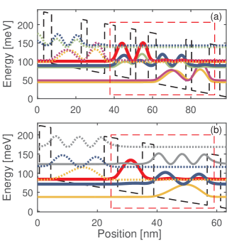
Figure 2: Conduction band profiles and probability densities of the investigated (a) four-well and (b) two-well THz QCL designs at a bias of $10\,\mathrm{kV}/\mathrm{cm}$ and $13\,\mathrm{kV}/\mathrm{cm}$, respectively. The main upper and lower laser level are marked by thick lines. The rectangles denote a single QCL period.

We apply the DM-EMC approach to two different THz QCL designs, the four-well LO phonon depopulation structure already shown in Fig. 1 where we focus on the design G951 with a sheet doping density of $1.2\times 10^{10}\,\mathrm{cm}^{-2}$,Benz et al. (2007) and a two-well photon-phonon structure Scalari et al. (2010). The conduction band diagrams of the two structures at lasing bias, obtained with a tight-binding Schrödinger-Poisson approach, are shown in Fig. 2.

We routinely consider four QCL modules, assuming periodic boundary conditions for the first and last one Iotti and Rossi (2001b), and simulate the coupled evolution of the carrier transport and optical cavity field over $70\,\mathrm{ps}$ to ensure convergence to steady state, using an ensemble of $10,000$ electrons. As pointed out in Section I, our main motivation behind DM-EMC is to increase the reliability and versatility of conventional EMC without sacrificing its relative computational efficiency. Our Fortran implementation of DM-EMC requires about $25$ minutes on a single thread of an Intel Xeon X5660 processor with a clock speed of $2.8\,\mathrm{GHz}$ for both the two- and the four-well design. The required memory is about $100\,\mathrm{MB}$ for the two-well and $150\,\mathrm{MB}$ for the four-well design per bias point, allowing parallel simulations of many bias points on a high performance server. This computational load is dominated by the evaluation of the scattering processes, and thus comparable to that of conventional EMC simulations.

III.1 Current-voltage characteristics

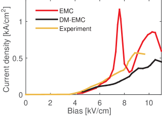
Figure 3: Comparison of simulated and experimental current-voltage characteristics for the four-well THz design at a lattice temperature of $77\,\mathrm{K}$. Shown are simulation results obtained with EMC and DM-EMC, and experimental data extracted from Ref. Benz et al., 2007.

In Fig. 3, the DM-EMC result for the current-voltage characteristics of the four-well THz QCL design is compared to semiclassical EMC results and available experimental data. DM-EMC shows good overall agreement with experiment. The computed peak current density is $0.48\,\mathrm{kA}/\mathrm{cm}^{2}$ at a bias of $10.5\,\mathrm{kV}/\mathrm{cm}$, as compared to $0.57\,\mathrm{kA}/\mathrm{cm}^{2}$ at $9\,\mathrm{kV}/\mathrm{cm}$ for the experiment. The slight deviations between simulation and measurement can partly be attributed to growth deviations of the experimental structure Benz et al. (2007). Furthermore, the exact amount of cavity loss is somewhat uncertain, since theoretical values extracted from waveguide modeling deviate significantly from experimental results obtained for similar QCL structures Benz et al. (2007). For our simulations, we assume waveguide and mirror power loss coefficients of $4\,\mathrm{cm}^{-1}$ and $3\,\mathrm{cm}^{-1}$, respectively, and a field confinement factor close to $1$ Benz et al. (2007); Ban et al. (2006); Kohen et al. (2005). The peak current density obtained by EMC in the lasing region is $0.86\,\mathrm{kA}/\mathrm{cm}^{2}$, significantly surpassing the experimental result. Furthermore, EMC produces a distinct spurious current spike of $1.17\,\mathrm{kA}/\mathrm{cm}^{2}$ at $7.6\,\mathrm{kV}/\mathrm{cm}$, which is almost four times higher than the experimental value of $0.31\,\mathrm{kA}/\mathrm{cm}^{2}$ at this bias. Such current spikes are well known artifacts of semiclassical EMC simulations Callebaut et al. (2003); Mátyás et al. (2010); Jirauschek et al. (2007), emerging at biases in the vicinity of small anticrossings. This scenario typically occurs for pairs of coupled states extending across thick injection barriers, which would in the semiclassical picture enable instantaneous electron tunneling across the barrier without resistance Callebaut and Hu (2005). This situation is illustrated in Fig. 1(a), where the corresponding extended wavefunctions are marked by bold lines. A suitable description of the tunneling transport is provided by the density matrix formalism of Section II.1, combined with the corresponding tight-binding wavefunctions as shown in Fig. 1(b). Here, tunneling is mediated by the coherent interaction between the left- and right-localized state, dampened by dephasing processes which can be modeled as described in Section II.2.

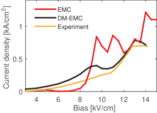
Figure 4: Comparison of simulated and experimental current-voltage characteristics for the two-well THz design at a lattice temperature of $10\,\mathrm{K}$. Shown are simulation results obtained with EMC and DM-EMC, and experimental data extracted from Ref. Scalari et al., 2010.

For further validation of DM-EMC, we have applied this approach to a two-well photon-phonon THz QCL design. Figure 4 contains the obtained current-voltage characteristics, along with the corresponding EMC and experimental results. For the simulation, we have assumed a total resonator loss coefficient of $15\,\mathrm{cm}^{-1}$, and again a field confinement factor close to $1$ Scalari et al. (2010); Kohen et al. (2005). The DM-EMC result agrees well with the experimental data, with an additional bump at around $9\,\mathrm{kV}/\mathrm{cm}$. Notably, such a feature has also been observed in NEGF simulations of this structure at the same bias, where it is attributed to tunneling through two barriers Wacker et al. (2013). The EMC simulation produces too low currents up to a bias of $8\,\mathrm{kV}/\mathrm{cm}$ and too high values above, caused by several extended current spikes which are due to narrow anticrossings of coupled states extending across the thick injection barrier.

III.2 Dephasing rates and subband electron distributions

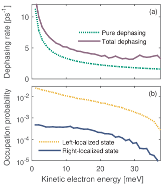
Figure 5: (a) Pure and total dephasing rate as a function of kinetic electron energy for the resonant tunneling transition across the thick barrier of the four-well QCL design at a bias of $7.6\,\mathrm{kV}/\mathrm{cm}$ and lattice temperature of $77\,\mathrm{K}$. (b) Occupation probability of the involved states, marked by bold lines in Fig. 1(b).

Figure 5(a) contains the pure and total dephasing rates as a function of kinetic electron energy $\varepsilon$ for the coupled state doublet mediating the tunneling transport across the injection barrier of the four-well design, marked in Fig. 1(b) by bold lines. The pure dephasing is obtained as a sum of the interface roughness and the impurity contribution, Eqs. (12) and (16). The total dephasing rate additionally contains the lifetime broadening contribution, computed based on the outscattering rate to states in other subbands Jirauschek and Lugli (2009). The occupation probabilities $f\left(\varepsilon\right)$ of the two subbands involved in the tunneling transition are shown in Fig. 5(b) on a logarithmic scale.

In one-dimensional DM QCL simulation approaches Kumar and Hu (2009); Dupont et al. (2010); Terazzi and Faist (2010); Dinh et al. (2012); Tzenov et al. (2016), the kinetic electron energy is not explicitly taken into account, and dephasing between two subbands $i$ and $j$ is often considered by an effective rate $\gamma_{ij}=\left(\gamma_{i}+\gamma_{j}\right)/2+\gamma_{ij}^{\prime}$, where $\gamma_{i}$ and $\gamma_{j}$ are the inverse electron lifetimes in subbands $i$ and $j$. The pure dephasing component $\gamma_{ij}^{\prime}$ is typically treated as an empirical or fitting parameter Kumar and Hu (2009); Dupont et al. (2010); Tzenov et al. (2016); Schrottke et al. (2010); Callebaut and Hu (2005), but can also be obtained from Ando’s model in Section II.2 by averaging over the inversion between the corresponding subbands Nelander and Wacker (2009); Freeman (2016). Assuming in-plane isotropy, we obtain with the in-plane wavevector $\mathbf{k}$, the kinetic electron energy $\varepsilon=\hbar^{2}k^{2}/\left(2m^{\ast}\right)$ and $k=\left|\mathbf{k}\right|$

$$\gamma_{ij}^{\prime} =\frac{\sum_{\mathbf{k}}\gamma_{ij,\mathbf{k}}^{\prime}\left|f_{i,\mathbf{k}}-f_{j,\mathbf{k}}\right|}{\sum_{\mathbf{k}}\left|f_{i,\mathbf{k}}-f_{j,\mathbf{k}}\right|}$$

$$\approx\frac{\int k\mathrm{d}k\gamma_{ij,k}^{\prime}\left|f_{i,k}-f_{j,k}\right|}{\int k\mathrm{d}k\left|f_{i,k}-f_{j,k}\right|}$$

$$=\frac{\int\mathrm{d}\varepsilon\gamma_{ij}^{\prime}\left(\varepsilon\right)\left|f_{i}\left(\varepsilon\right)-f_{j}\left(\varepsilon\right)\right|}{\int\mathrm{d}\varepsilon\left|f_{i}\left(\varepsilon\right)-f_{j}\left(\varepsilon\right)\right|}.$$ (17)

For the case depicted in Fig. 5, Eq. (17) yields a pure dephasing rate $\gamma_{ij}^{\prime}=4.62\,\mathrm{ps}^{-1}$ and a lifetime broadening contribution of $1.74\,\mathrm{ps}^{-1}$, resulting in $\gamma_{ij}=6.36\,\mathrm{ps}^{-1}$. Next, we investigate dephasing in the four- and the two-well QCL design at the lasing biases considered in Fig. 2. For the pair of tunneling states with the narrowest anticrossing, we obtain $\gamma_{ij}^{\prime}=2.04\,\mathrm{ps}^{-1}$, $\gamma_{ij}=2.69\,\mathrm{ps}^{-1}$ for the four-well structure, and $\gamma_{ij}^{\prime}=2.02\,\mathrm{ps}^{-1}$, $\gamma_{ij}=3.82\,\mathrm{ps}^{-1}$ for the two-well design. These obtained values of $\gamma_{ij}^{\prime}$ are consistent with the expected pure dephasing times $\left(\gamma_{ij}^{\prime}\right)^{-1}\sim 0.3..1\,\mathrm{ps}$, deduced from measurements and fits to experimental data Freeman (2016); Kumar and Hu (2009); Dupont et al. (2010); Callebaut and Hu (2005). For the main lasing transition, the dephasing rates are $\gamma_{ij}^{\prime}=0.24\,\mathrm{ps}^{-1}$, $\gamma_{ij}=2.37\,\mathrm{ps}^{-1}$ for the four-well structure, and $\gamma_{ij}^{\prime}=0.75\,\mathrm{ps}^{-1}$, $\gamma_{ij}=3.17\,\mathrm{ps}^{-1}$ for the two-well design, corresponding to full width at half-maximum Lorentzian gain bandwidths $\gamma_{ij}/\pi$ of $0.76\,\mathrm{THz}$ and $1.01\,\mathrm{THz}$, respectively. As expected, for the lasing transitions pure dephasing has a much smaller impact than for the tunneling transport across thick barriers Dupont et al. (2010), justifying the use of lifetime broadening approaches to calculate spectral gain bandwidths in QCLs Jirauschek and Lugli (2009). One reason is that the pure dephasing contribution $\gamma_{ij}^{\prime}$ tends to become small if there is a considerable overlap between the corresponding wavefunctions, e.g., for vertical lasing transitions, since then the matrix elements in Eq. (7) partially cancel Dupont et al. (2010). With sheet doping densities of $1.2\times 10^{10}\,\mathrm{cm}^{-2}$ and $1.5\times 10^{10}\,\mathrm{cm}^{-2}$ for the four- and two-well design, respectively, and assuming typical interface roughness parameters of $\Delta=0.12\,\mathrm{nm}$, $\Lambda=10\,\mathrm{nm}$ Nelander and Wacker (2008), the pure dephasing rates given above are dominated by impurity scattering, which contributes at least 70% to $\gamma_{ij}^{\prime}$. Additionally, we have verified that an inclusion of LO phonons would have modified above values of $\gamma_{ij}^{\prime}$ by less than 4%, justifying the omission of LO phonon contributions for the evaluation of pure dephasing in such types of QCL designs Freeman (2016). Instead of computing the lifetime broadening contribution $\left(\gamma_{i}+\gamma_{j}\right)/2$ from the inverse electron lifetimes $\gamma_{i}$ and $\gamma_{j}$ in subbands $i$ and $j$, respectively, an alternative approach would be to take the corresponding term $(\gamma_{i,\mathbf{k}}+\gamma_{j,\mathbf{k}})/2$  from Eq. (5), and average it in the same way as $\gamma_{ij,\mathbf{k}}^{\prime}$, by using Eq. (17). This leads to different results for transitions between subbands with non-identical electron temperatures or even non-thermal kinetic energy distributions. However, for the examples discussed above, both approaches yield similar values for the total linewidth $\gamma_{ij}$ to within 10%.

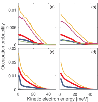
Figure 6: Subband electron distributions at lasing bias for the four-well QCL design at operating temperatures of (a) $10\,\mathrm{K}$ and (b) $147\,\mathrm{K}$, and for the two-well design at (c) $10\,\mathrm{K}$ and (d) $125\,\mathrm{K}$. The applied bias fields and line coding of the subbands are as in Fig. 2(a) and (b), respectively.

The electron distributions of the localized tunneling states shown in Fig. 5(b) are for a bias of $7.6\,\mathrm{kV}/\mathrm{cm}$, where a narrow anticrossing of these states occurs (see Fig. 1). Here, almost all electrons in this subband doublet are localized to the left of the barrier, which is the opposite scenario as assumed in the semiclassical picture, where instantaneous tunneling results in equal population distributions to the left and the right of the barrier Callebaut and Hu (2005). This observation is consistent with the breakdown of semiclassical EMC at this bias point, leading to the current spike shown in Fig. 3. In Fig. 6, the subband electron distributions of the four- and the two-well design are displayed at lasing bias for low ($10\,\mathrm{K}$) and the maximum experimentally achieved ($147\,\mathrm{K}$ and $125\,\mathrm{K}$ Benz et al. (2007); Scalari et al. (2010), respectively) operating temperatures. For the four-well structure, there are considerably less electrons in the right-localized tunneling state [the third highest occupied level in Fig. 6(a) and (b)] than in the closely aligned left-localized state (the highest occupied level), similarly as for the case shown in Fig. 5(b). Again, the current density obtained with EMC at the corresponding bias point of $10\,\mathrm{kV}/\mathrm{cm}$ in Fig. 3 is too high since the piling up of electrons behind the thick barrier is not contained in the semiclassical description. By contrast, for the two-well design the occupation in both tunneling states [the two highest occupied levels in Fig. 6(c) and (d)] is comparable, and the EMC result for the current density at the corresponding bias of $13\,\mathrm{kV}/\mathrm{cm}$ in Fig. 4 agrees well with the DM-EMC simulation. Equivalent electronic subband temperatures can be extracted from the expectation values of the kinetic electron energy Shi and Knezevic (2014); Ezhov and Jirauschek (2016). These are in the range of $121\,\mathrm{K}-145\,\mathrm{K}$ [Fig. 6(a)], $160\,\mathrm{K}-199\,\mathrm{K}$ [Fig. 6(b)], $116\,\mathrm{K}-127\,\mathrm{K}$ [Fig. 6(c)], and $154\,\mathrm{K}-165\,\mathrm{K}$ [Fig. 6(d)], significantly exceeding the lattice temperature (which corresponds to the operating temperature at low duty cycles). This is the well known hot electron effect, which has also been experimentally observed for resonant phonon THz QCLs Vitiello et al. (2005). We note that the subband electron distributions deviate, in part, significantly from heated Maxwellian distributions. In particular, the lower laser level distribution of the two-well structure [third highest occupied level in Fig. 6(c) and (d)] is highly non-Maxwellian, since its energetic distance of $33.5\,\mathrm{meV}$ to the ground level is below the LO phonon energy of $36\,\mathrm{meV}$. Consequently, the LO phonon depopulation channel is blocked for electrons at the bottom of the lower laser level. While, as mentioned above, the piling up of electrons behind thick tunneling barriers can only be modeled by considering quantum coherence effects, hot electrons and non-Maxwellian subband carrier distributions are also adequately described by semiclassical simulations Iotti and Rossi (2001b); Callebaut et al. (2004); Jirauschek and Lugli (2008); Iotti et al. (2010); Shi and Knezevic (2014).

IV Conclusion

In conclusion, we have presented a DM-based method to self-consistently include incoherent tunneling into the EMC framework for QCL simulations. The resulting DM-EMC approach maintains the strengths of EMC, such as its relative computational efficiency and the inclusion of intercarrier scattering as well as carrier-light coupling, while partially curing the main shortcoming of semiclassical QCL modeling techniques, i.e., the omission of quantum coherence effects. Out of these, tunnel coupling between state doublets spanning thick barriers plays an eminent role. For narrow anticrossings of the tunneling states, as especially occur in THz QCL designs with thick injection barriers, a semiclassical treatment can even break down completely, which manifests itself in the emergence of an artificial spike in the current-voltage characteristics. By a self-consistent implementation of tunnel dephasing based on Ando’s model, we have in our approach eliminated the need for empirical dephasing times. We have validated our simulation scheme against experimental data for a two- and a four-well THz QCL design, clearly demonstrating the superiority of DM-EMC over conventional EMC for those structures. The developed approach is not only relevant for steady-state QCL simulations, but will also be useful for Maxwell-Bloch-type modeling of the QCL dynamics where a coupling to steady-state carrier transport simulations can yield the required scattering and dephasing rates Tzenov et al. (2016, 2017).