SF2A 2017

Non-adiabatic oscillations of fast-rotating stars: the example of Rasalhague

Early-type stars generally tend to be fast rotators. In these stars, mode identification is very challenging as the effects of rotation are not well known. We consider here the example of $\alpha$ Ophiuchi, for which dozens of oscillation frequencies have been measured. We model the star using the two-dimensional structure code ESTER, and we compute both adiabatic and non-adiabatic oscillations using the TOP code. Both calculations yield very complex spectra, and we used various diagnostic tools to try and identify the observed pulsations. While we have not reached a satisfactory mode-to-mode identification, this paper presents promising early results.

1 Introduction

In many early-type (O-,B- and A-type) stars, the $\kappa$-mechanism excites both pressure and gravity modes. These stars are also usually fast rotators, with an average $v\sin i\sim 100-200{\mathrm{km~{}s^{-1}}}$ (Royer 2009). The impact of this rotation is twofold: the star is flattened by the centrifugal force, while the Coriolis acceleration modifies the mode properties. Both of those effects scramble the oscillation spectra and make mode identification much harder, requiring two-dimensional stellar models and oscillation calculations.

In this work, we extend the work by Mirouh et al. (2013) by using the so-called forward approach to model the fast rotator Rasalhague ($\alpha$ Ophiuchi). We model the star using the two-dimensional code ESTER that fully takes rotation into account, but leaves out mass loss and chemical diffusion in the star, and then compute the non-perturbative oscillation spectrum in the same geometry using the TOP program. Due to the high resolution used to describe the stellar interior and the modes, this typically yields several hundreds of modes, among which we need to select the most relevant candidates for identification. Another approach consists in looking for regular patterns in the oscillation spectrum: because of the effects of rotation, theoretically-predicted patterns (Lignières & Georgeot 2009) went long unnoticed, until García Hernández et al. (2015) was able to find a large separation in a small sample of stars and link it to stellar properties.

2 Rasalhague

Our study case is the A-type star Rasalhague. Interferometry showed that the star is seen almost equator-on, with a ratio between the equatorial and polar radii of $1.2$, i.e. $R({\rm pole})=1.2R({\rm equator})$ (Zhao et al. 2009). Its mass has been constrained by means of its orbiting companion (Hinkley et al. 2011) and interferometry to $M\sim 2.18-2.4M_{\odot}$. Moreover, fifty-seven oscillation frequencies, ranging from $1.768$ to $48.347$ c/d, have been measured with the asteroseismology mission MOST (Monnier et al. 2010).

We compute an ESTER model (Espinosa Lara & Rieutord 2013; Rieutord et al. 2016) that fits the luminosity and the equatorial and polar radii, the properties of which are summarized in table 1. This model is the same as the one presented in Mirouh et al. (2013).

$$\begin{array}[]{|c|c||c|c|}\hline\cr\Omega/\Omega_{K}&0.624&T_{\rm eff}(p)(K)&9177\\ M/M_{\odot}&2.22&T_{\rm eff}(e)(K)&7731\\ X_{c}/X&0.3685&R(p)/R_{\odot}&2.388\\ X&0.7&R(e)/R_{\odot}&2.858\\ Z&0.02&V_{\rm eq}({\rm km.s}^{-1})&240\\ &&L/L_{\odot}&31.1\\ \hline\cr\end{array}$$

Table 1: Properties of our model for Rasalhague ($\alpha$ Ophiuchi). The left part of the table contains the input parameters of the model, while the right part lists the quantities matched to the quantities observed for the star.

3 Adiabatic oscillations

The eigenvalue problem of adiabatic oscillations is solved with the TOP code (Reese et al. 2009) for modes with azimuthal orders $-4\leq m\leq 4$, in the range of frequencies in which modes are observed. We find g modes and p modes modified by rotation, and we can clearly distinguish these two populations in the spectra (see Figure 1).

To select the modes that might be seen from Earth, we compute the mode visibilities, following Reese et al. (2013). As the mode amplitudes cannot be derived from a linear calculation, we need to normalize the eigenmodes. For this purpose, we normalize all our solutions by $\max||\mbox{\boldmath{$\xi$}}||^{2}\left(\omega+m\Omega\right)^{2}$, where $\xi$ is the Lagrangian displacement and $\left(\omega+m\Omega\right)$ the corotating mode frequency (Reese et al. 2017). We find that g modes are the least visible, as one would expect, considering they probe deep layers of the star and are usually evanescent towards the surface. Located near the surface, p modes are much more visible.

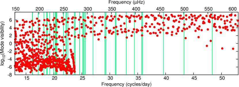
Figure 1: Mode visibilities of $m=0$ modes, obtained through adiabatic calculations. The low-frequency low-visibility clump corresponds mostly to g modes, while the higher-visibility strip spanning the whole frequency range corresponds to p modes. Each vertical green line corresponds to a frequency measured by Monnier et al. (2010).

We also compute the thermal dissipation rates using the quasi-adiabatic approximation (Unno et al. 1989), which yields only linearly stable modes. Using this method, the more visible p modes appear to be more damped than the g modes. This conundrum seems to prevent the identification of the modes.

4 Non-adiabatic oscillations

In an attempt to improve our description of the modes, we use the non-adiabatic version of TOP (Reese et al. 2016). This calculation is much more demanding numerically but results in complex eigenvalues that include both the modes’ frequencies and growth rates. While the mode visibilities present the same properties as that of the adiabatic modes shown in figure 1, we are able to find amplified modes. Figure 2 shows the growth rates of the modes. Keeping only the most visible amplified modes does not seem to allow a direct identification of the modes, but fine tuning the models might lead to a better match. The ESTER models also suffer from a couple of limitations that may affect our calculation: as of now, the code does not implement evolution but determines the stellar structure at a given time; it also leaves aside any surface convection. As this prevents us from describing accurately the transfer of heavy elements from the core to the envelope due to core recession or diffusive effects along the main-sequence evolution, and results in a two-domain chemical composition with a depleted core and a homogeneous envelope, it may impact individual eigenmodes, and especially the g modes that probe deep layers in the star.

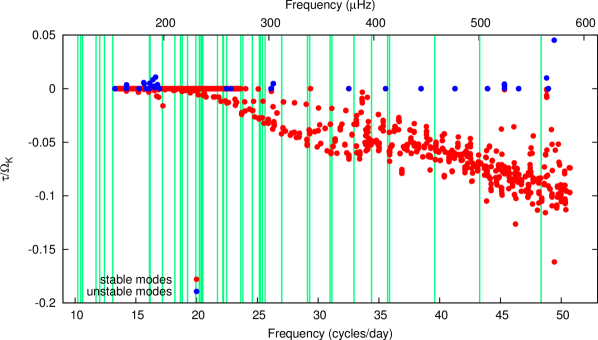
Figure 2: Damping rates for the axisymmetric modes ($m=0$) obtained through the non-adiabatic calculation. We find amplified g and p modes, most of the latter seem to follow a regular pattern.

We also find a series of amplified modes that seem spaced by a regular separation. However, this separation is not exactly constant ($\sim 30\mu$Hz) and does not seem to match the one uncovered by García Hernández et al. (2015) ($20\pm 1\mu$Hz). When checking the nature of the modes, it appears that these amplified modes are high-degree gravity modes, and not the island pressure modes hypothesized by Lignières & Georgeot (2009).

Two-dimensional non-adiabatic calculations are still at an early stage, and the needed resolution, associated with the high number of variables and equations involved, impact the precision of the solutions. To improve the numerical convergence, we decide to split the star in two domains: we solve the perturbed equations using the adiabatic approximation in the inner part of the star, while the full non-adiabatic equations are solved in the outer part. For a first exploration, we set the Lagrangian perturbation of entropy to zero at the interface between the two domains. Figure 3 shows the dispersion of the solutions for various sizes of the inner adiabatic domain, for the p mode at $f=424.378\mu$Hz when using slightly different input guesses.

We see that as we move the interface outwards, the solutions first get closer to the average value (that we suppose to be correct): this is explained by the disappearance of numerical errors, as the very small $\delta s$ is no longer computed in the inner part of the star but set to zero by hand. However, when the adiabatic region becomes larger, the growth rate gradually falls to zero, as we start neglecting non-adiabatic effects that are important in outer layers.

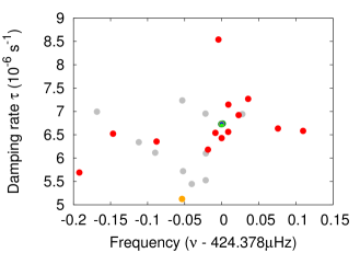
Figure 3: The left plot shows the dispersion for the split calculation. We place the adiabatic inner domain/non-adiabatic outer domain interface at various depths, shown on the meridional cut on the right plot. The colours of the symbols correspond to those of the interfaces: the grey points corresponding to the full non-adiabatic calculation, while the dark green, yellow, blue and green dots overlap. We omit the result of the fully adiabatic calculation, which would have $\tau=0$.

5 Conclusions and future prospects

In this work, we computed a two-dimensional model and both the adiabatic and non-adiabatic oscillations of the fast-rotating $\delta$ Scuti star $\alpha$ Ophiuchi, in order to identify the observed oscillation frequencies. Because of the complexity of the oscillation spectrum, and the high number of calculated eigenmodes, we computed the damping rates and mode visibilities in order to narrow down the range of possible matches between calculated and observed modes. The adiabatic calculation, using the so-called quasi-adiabatic approximation predicts only damped modes. This is due to a poor description of the modes near the stellar surface. Using a non-adiabatic calculation allows us to find amplified modes. As we cannot predict the amplitude of the modes, we normalize them and compute their visibilities. Using these two diagnostics, we are able to select only a reasonably small subsample of the whole synthetic spectrum, that we compare to the observations. At this point, we were unable to identify individual frequencies or find regular patterns that match the observations. This may come from the numerical issues raised by the non-adiabatic calculation or the limitations of the ESTER stellar models. Improving both of these aspects will be necessary to make the oscillation growth rates and the rotating star structures more reliable and reach a satisfying two-dimensional seismic inference for Rasalhague.

References

- Espinosa Lara & Rieutord (2013) Espinosa Lara, F. & Rieutord, M. 2013, A&A, 552, A35
- García Hernández et al. (2015) García Hernández, A., Martín-Ruiz, S., Monteiro, M. J. P. F. G., et al. 2015, ApJ Lett., 811, L29
- Hinkley et al. (2011) Hinkley, S., Monnier, J. D., Oppenheimer, B. R., et al. 2011, ApJ, 726, 104
- Lignières & Georgeot (2009) Lignières, F. & Georgeot, B. 2009, A&A, 500, 1173
- Mirouh et al. (2013) Mirouh, G. M., Reese, D. R., Espinosa Lara, F., Ballot, J., & Rieutord, M. 2013, in IAU Symposium 301, Vol. 865, Precision Asteroseismology, ed. W. Chaplin, J. Guzik, G. Handler, & A. Pigulski, 1
- Monnier et al. (2010) Monnier, J. D., Townsend, R. H. D., Che, X., et al. 2010, ApJ, 725, 1192
- Reese et al. (2016) Reese, D. R., Dupret, M.-A., & Rieutord, M. 2016, in Seismology of the Sun and the Distant Stars 2016, ed. M. J. P. F. G. Monteiro, M. S. Cunha, & J. M. T. Ferreira
- Reese et al. (2017) Reese, D. R., Lignières, F., Ballot, J., et al. 2017, A&A, 601, A130
- Reese et al. (2013) Reese, D. R., Prat, V., Barban, C., van ’t Veer-Menneret, C., & MacGregor, K. B. 2013, A&A, 550, A77
- Reese et al. (2009) Reese, D. R., Thompson, M. J., MacGregor, K. B., et al. 2009, A&A, 506, 183
- Rieutord et al. (2016) Rieutord, M., Espinosa Lara, F., & Putigny, B. 2016, Journal of Computational Physics, 318, 277
- Royer (2009) Royer, F. 2009, in Lecture Notes in Physics, Berlin Springer Verlag, Vol. 765, The Rotation of Sun and Stars, ed. J.-P. Rozelot & C. Neiner, 207–230
- Unno et al. (1989) Unno, W., Osaki, Y., Ando, H., Saio, H., & Shibahashi, H. 1989, Nonradial oscillations of stars (University of Tokyo Press)
- Zhao et al. (2009) Zhao, M., Monnier, J. D., Pedretti, E., et al. 2009, ApJ, 701, 209