Deep Matching Autoencoders

Abstract

Increasingly many real world tasks involve data in multiple modalities or views. This has motivated the development of many effective algorithms for learning a common latent space to relate multiple domains. However, most existing cross-view learning algorithms assume access to paired data for training. Their applicability is thus limited as the paired data assumption is often violated in practice: many tasks have only a small subset of data available with pairing annotation, or even no paired data at all.

In this paper we introduce Deep Matching Autoencoders (DMAE), which learn a common latent space and pairing from unpaired multi-modal data. Specifically we formulate this as a cross-domain representation learning and object matching problem. We simultaneously optimise parameters of representation learning auto-encoders and the pairing of unpaired multi-modal data. This framework elegantly spans the full regime from fully supervised, semi-supervised, and unsupervised (no paired data) multi-modal learning. We show promising results in image captioning, and on a new task that is uniquely enabled by our methodology: unsupervised classifier learning.

1 Introduction

Learning representations from multi-modal data is a widely relevant problem setting in many applications of machine learning and pattern recognition. In computer vision it arises in tagging [11, 16], cross-view [15, 27] and cross-modal [38] learning. It is particularly relevant at the border between vision and other modalities, for example audio-visual speech classification [36] and generating descriptions of images and videos [8, 18, 19, 30, 37] in the case of audio and text respectively.

The wide applicability of multi-modal representation learning has motivated the study of numerous cross-modal learning methods including Canonical Correlation Analysis (CCA) [21, 23] and Kernel CCA [3]. Progress has further accelerated recently with the contribution of large parallel datasets [34, 49], which have permitted the application of deep multi-modal models such as DeepCCA [2] and other two branch deep networks to tasks such as image-caption matching [45] and zero-shot learning [12]. Nevertheless a pervasive limitation of all these methods is that they are fully supervised methods in the sense that they require paired training data to learn the cross-modal mapping or embedding space. However, in many applications paired data may be relatively sparse compared to unpaired data, in which case semi-supervised cross-modal learning methods would be beneficial to exploit the abundant unpaired data. Moreover, in some cases it may be desirable to learn from pools of data in each modality which are completely unpaired, necessitating unsupervised cross-modal learning.

In this paper we address the task of cross-modal learning from partially or completely unpaired data. There have been only a few prior attempts to address inferring pairings from partially or completely unmatched data. These include Kernelized sorting (KS) [10, 26, 39], least-square object matching (LSOM) [46, 47], and matching CCA (MCCA) [20]. However these existing algorithms are all shallow and thus may not perform well on challenging complex data where representation learning is important, such as images and text. We introduce Deep Matching Autoencoders (DMAE), which to our knowledge provide the first deep representation learning approach to unpaired cross-modal learning.

Our  DMAE method employs an auto-encoder model for each data view, which are learned by minimizing reconstruction error as usual. We further introduce a latent alignment matrix to model the unknown pairing between views, which we optimize using cross-modal dependency measures kernel target alignment (KTA) [9] and squared-loss mutual information (SMI) [46]. With this framework we simultaneously learn the autoencoding representation and the cross-view pairing. In this way the representation is trained to support cross-view matching. During training the learned representation improves as cross-view matching is progressively disambiguated, and cross-modal items are paired more accurately as the learned representation progressively improves.

Our proposed framework elegantly spans the spectrum from fully supervised to fully unsupervised cross-modal learning. The fully supervised case corresponds to conventional cross-modal learning, where our approach is an alternative to DeepCCA [2] or two branch matching nets [45], except that we use a statistical dependency-based rather than correlation or ranking-based loss. We show that our approach performs comparably to state of the art alternatives for supervised tasks. More interestingly, our approach is effective for semi-supervised learning (only subset of pairings available), and we show that it is able to better exploit unlabeled multi-modal data to improve performance compared to alternatives such as matching CCA [20]. Most interestingly, our approach is even effective for unsupervised cross-modal learning where no pairings are given. We demonstrate this capability by introducing and solving a novel task termed unsupervised classifier learning (UCL).

In the UCL task we assume a pool of unlabelled images are given along with a pool of category embeddings (e.g., word-vectors) that describe the images in the pool. However it is unsupervised in that no pairings between images and categories are given. This task corresponds to an application where we have a pool of images and we have some idea of the classes likely to be represented in those images; but no specific class-image pairings. Based on these inputs alone we can train classifiers to recognise the categories represented in the category embedding pool. Like the classic clustering problem, this task is unsupervised in that there is no supervision/pairing given. However like the conventional supervised learning setting, UCL produces classifiers for specific nameable image categories as an output. This task can be seen as an extreme version of zero-shot learning [32, 43], where there is no auxiliary set with image + class embedding pairs available to learn an image-category embedding mapping. The image-category mapping must be learned in an entirely unsupervised way.

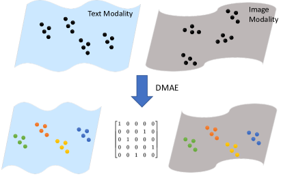
Figure 1: Multimodal learning from unpaired data problem setting. DMAE inputs a set of unpaired instances in each view and learns: (i) A permutation matrix associating objects across views. (ii) A new representation for each with maximum statistical dependency.

Our contributions can be summarized as follows:

• We propose DMAE, a cross-view learning and matching framework that elegantly spans supervised, semi-supervised and unsupervised cross-modal learning.

• Our framework performs comparably to state of the art on the topical image-caption matching benchmark.

• DMAE  is effective in leveraging unpaired data in a semi-supervised setting, and learning entirely from unpaired data in an unspervised setting.

• We introduce and provide a first solution to the the novel problem of unsupervised classifier learning.

2 Related Work

2.1 Multi-modal learning

Many modern digital events are inherently multimodal in nature, i.e a video or image that you favourite is followed with a caption, a tag or comment. In most supervised multi-modal learning setups, it is a privilege to have access to paired data (i.e., $\{({\bm{x}}_{i},{\bm{y}}_{i})\}_{i=1}^{n}$). For example where ${\bm{x}}$ is a vector of image and ${\bm{y}}$ is a vector of text. In unsupervised multi-modal learning setup, we can only access to unpaired data $\{{\bm{x}}_{i}\}^{n}_{i=1}$ and $\{{\bm{y}}_{j}\}^{n}_{j=1}$. The semi-supervised setup is a mixture of the supervised and unsupervised setup.

Supervised multi-modal learning  The most established supervised multi-modal learning algorithm is canonical correlation analysis (CCA) [23], which learns a linear projection of features in two views such that are maximally correlated in a common latent space. CCA has been studied extensively and has a number of useful properties [21]. In particular, the optimal linear projection mapping can be obtained by solving an eigenvalue decomposition. It has also been extended to the non-linear case via kernelization (KCCA) [3].

The huge success of deep neural network (DNN) in computer vision and NLP has inspired many deep multi-modal learning algorithms including DeepCCA [2], multi-modal deep autoencoders (DAEs) [11, 36], and two branch matching or ranking networks [45]. DeepCCA [2] shares the correlation maximizing objective with classic CCA, but learns a non-linear projection via deep neural networks. It has been shown to outperform linear CCA and its non-linear KCCA extension. In multi-modal DAEs [36] multi-modal autoencoders are trained with a shared hidden layer. More generally paired data has been used to train two branch DNNs to learn view-invariant embeddings for example via a learning to rank [12, 45] objective.

In contrast to these Euclidean-based metrics, statistical dependency-based measures have like the Hilbert-schmidt independence criterion (HSIC) [17] have been much less studied as objectives for multi-modal learning. One example is HSIC-CCA [5], which learned a CCA type architecture but with HSIC rather than correlation objective.

However, the above supervised algorithms – particularly the deep learning ones – require a large number of paired samples to learn an effective cross-modal embedding.

Unsupervised multi-modal learning  The desirability of learning from more widely available unpaired data has motivated some research into the harder problem of unsupervised cross-modal learning by introducing latent variables for cross-view pairing. An early approach was Matching CCA [20]. It alternates between learning a joint embedding space with CCA, and solving a bipartite matching problem to associate the unpaired data. Unlike the statistical dependency measures, CCA’s correlation-based objective requires comparable embeddings to estimate a match. So Matching CCA can never bootstrap itself if initialised with completely random embeddings and no pairing information at all. Indeed it was only shown to work when used with a seed of paired samples for bootstrapping [20] – i.e., in the semi-supervised setting. Probabilistic latent variable approaches have also been proposed to match across-views [24], however this was only demonstrated to work on toy problems. Both of these are limited to linear projections.

To handle non-linearity in unsupervised multi-modal learning, kernel based approaches were proposed including Kernelized sorting (KS) [10, 26, 39] and the least-squared object matching [46, 47]. In KS, unpaired data are matched by maximizing HSIC, and it has outperformed MCCA on NLP tasks [25]. In LSOM, squared-loss mutual information (SMI) is used as a dependence measure, and it was experimentally shown to outperform the HSIC-based KS. However, both KS and LSOM are shallow methods, so may not perform well for image and text data where representation learning is beneficial. In this paper we leverage HSIC and SMI-based objectives for learning representations for matching in a deeper context.

2.2 Applications

Visual Description with Natural Language  Generating or matching natural language descriptions for images and videos has recently become a popular topic in cross-modal learning in the last five years [37]. A common approach is to learn an image representation (e.g., CNN), a text representation (e.g., Bag of Words or LSTM [22]) and then map these into a common latent space via two-branch deep networks [29, 45, 48]. Based on this latent space, images or videos and associated text descriptions can be matched: supporting annotation or retrieval applications. Our proposed  DMAE  solves supervised image captioning comparably well to the state of the art methods. But unlike prior approaches it can be generalized to the semi-supervised and unsupervised case for exploiting unpaired data.

Zero-shot learning  Zero-shot learning (ZSL) aims to improve the scalability of visual classifier learning in terms of the required image annotation. Specifically, it assumes that a subset of image categories (‘seen’ categories) are provided with example images (i.e., annotations), and aims to generate classifiers for a disjoint set of image categories (‘unseen’ categories) that have no example images. This is achieved by further assuming that all image categories have an associated category embedding vector, for example word-vectors [35] or attributes [33]. Given this assumption a cross-modal mapping can be learned from visual feature space to category embedding space using the data for seen classes. The cross-modal mapping can then be used as a classifier in order to recognise those unseen categories for which no annotated examples were provided [12, 41].

Our  DMAE approach is related to ZSL methods in that it can be applied to learn cross-modal embeddings between images and category vectors, and hence it can also be used as a classifier for novel classes. However it has a few crucial benefits: (i) It can be learned in a semi-supervised way, which encompasses the transductive [14, 43] and semi-supervised [43] variants of ZSL. (ii) More interestingly, it can also be learned in an entirely un-supervised way – requiring no paired samples at all; unlike all existing ZSL methods. We term this specific problem setting  unsupervised classifier learning (UCL).

A recent ZSL method ReViSE [43] is related to ours in that it can also benefit from the semi-supervised learning setting via a HSIC-based domain adaptation loss. However ReViSE is engineered specifically for ZSL. In contrast our  DMAE is a general cross-modal learner, and can address the completely unsupervised setting unlike ReViSE.

3 Matching Deep Autoencoders

We introduce our cross-domain object matching methodology, Deep Matching Autoencoders (Figure 2) from the unsupervised learning perspective where no paired training data is assumed. From here semi-supervised and supervised variants are a straightforward special case. For exposition simplicity we also assume an equal number of samples in each view, but this can be relaxed in practice.

3.1 Multi-View Autoencoders

Consider two unpaired sets of samples, $\{{\bm{x}}_{i}\}_{i=1}^{n}$ and $\{{\bm{y}}_{i}\}_{i=1}^{{n}}$, where ${\bm{x}}\in\mathbb{R}^{d_{x}}$ and ${\bm{y}}\in\mathbb{R}^{d_{y}}$. For example, ${\bm{x}}$ is a feature vector extracted from an image and ${\bm{y}}$ is a vector representation of a text. We assume a heterogeneous setup; the dimensionality of ${\bm{x}}$ and ${\bm{y}}$ are completely different.

Let us denote the autoencoders of ${\bm{x}}$ and ${\bm{y}}$ as

$${\bm{f}}_{{\bm{x}}}({\bm{g}}_{{\bm{x}}}({\bm{x}};{\bm{\Theta}}_{{\bm{x}}});{\bm{\Theta}}_{{\bm{x}}}),~{}~{}~{}{\bm{f}}_{{\bm{y}}}({\bm{g}}_{{\bm{y}}}({\bm{y}};{\bm{\Theta}}_{{\bm{y}}});{\bm{\Theta}}_{{\bm{y}}}),$$

where ${\bm{g}}(\cdot)$ is an encoder and ${\bm{f}}(\cdot)$ is a decoder function, ${\bm{\Theta}}_{{\bm{x}}}$, and ${\bm{\Theta}}_{{\bm{y}}}$ are the autoencoder parameters.

Our goal is to learn comparable representation embeddings $\bm{g}_{x}(\cdot)$ and $\bm{g}_{y}(\cdot)$ given no paired training data. This is a significantly harder problem than other multi-modal autoencoder approaches that rely on paired data [4, 36].

3.2 Learning from Unpaired Data

To learn from unpaired data we introduce a permutation matrix to represent the unknown correspondence between data items in two views [39, 47, 46]. Let $\pi$ be an permutation function over $\{1,2,\ldots,n\}$, and let ${\bm{\Pi}}$ be the corresponding permutation indicator matrix:

$${\bm{\Pi}}\in\{0,1\}^{n\times n},{\bm{\Pi}}{\bm{1}}_{n}={\bm{1}}_{n},\text{and}~{}{\bm{\Pi}}^{\top}{\bm{1}}_{n}={\bm{1}}_{n},$$

where ${\bm{1}}_{n}$ is the $n$-dimensional vector with all ones.

Then, we consider the following optimization problem:

$$\min_{{\bm{\Theta}}_{{\bm{x}}},{\bm{\Theta}}_{{\bm{y}}},{\bm{\Pi}}}\sum_{i=1}^{n}\|{\bm{x}}_{i}-{\bm{f}}_{{\bm{x}}}({\bm{g}}_{{\bm{x}}}({\bm{x}}_{i}))\|_{2}^{2}+\|{\bm{y}}_{i}-{\bm{f}}_{{\bm{y}}}({\bm{g}}_{{\bm{y}}}({\bm{y}}_{i})))\|_{2}^{2}$$

$$\phantom{\min_{{\bm{\Theta}}_{{\bm{x}}},{\bm{\Theta}}_{{\bm{y}}},{\bm{\Pi}}}}-\lambda D_{\Pi}(\{{\bm{g}}_{{\bm{x}}}({\bm{x}}_{i}),{\bm{g}}_{{\bm{y}}}({\bm{y}}_{\pi(i)})\}_{i=1}^{n}),$$ (1)

where we are simultaneously optimising the autoencoders (${\bm{\Theta}}_{{\bm{x}}}$ and ${\bm{\Theta}}_{{\bm{y}}}$ ) as well as the cross-domain match (${\bm{\Pi}}$) with tradeoff parameter $\lambda$. The key component here is the function $D_{{\bm{\Pi}}}(\cdot,\cdot)$ which is a non-negative statistical dependence measure between the $x$ and $y$ views. $D_{{\bm{\Pi}}}(\cdot,\cdot)$ needs to be a measure which does not require comparable representations a priori in order to enable learning to get started.

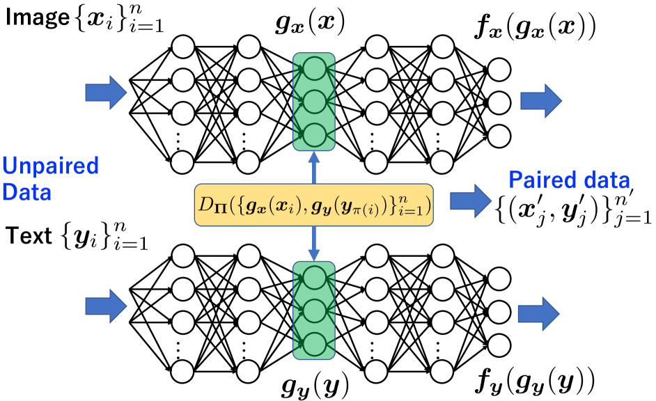
Figure 2: Model Architecture of DMAE.

3.3 Dependence Measures

The statistical dependence measure is the crucial component in achieving our goal. In this paper, we explore two alternatives: the unnormalized kernel target alignment (KTA) [9] and the squared-loss mutual information (SMI) [42, 46, 47]. Note that SMI is an independence measure. However, since we want to make ${\bm{\Theta}}_{\bm{x}}$ and ${\bm{\Theta}}_{\bm{y}}$ generate similar representations, we use SMI as a dependence measure.

Unnormalized kernel target alignment (uKTA)  In uKTA [9], we consider the following similarity function $D$ for paired data:

$$\text{uKTA}(\{({\bm{x}}_{i},{\bm{y}}_{i})\}_{i=1}^{n})=\text{tr}\left({\bm{K}}{\bm{L}}\right),$$

where $\text{tr}(\cdot)$ is the trace operator, ${\bm{K}}$ is the Gram matrix for ${\bm{x}}$ and ${\bm{L}}$ is the Gram matrix for ${\bm{y}}$. This similarity function takes large value if the Gram matrices ${\bm{K}}$ and ${\bm{L}}$ are similar, and a small value if they are not similar. Note that, in the original KTA, we have the normalization term. However, this makes the optimization hard, and thus we employ the unnormalized variant of KTA. Moreover, uKTA can be regarded as a non-centered variant of HSIC [17].

We use the Gaussian kernel:

$${\bm{K}}_{ij}\!\!=\!\exp\left(-\frac{\|{\bm{x}}_{i}-{\bm{x}}_{j}\|_{2}^{2}}{2\sigma_{x}^{2}}\right),~{}{\bm{L}}_{ij}\!\!=\!\exp\left(-\frac{\|{\bm{y}}_{i}-{\bm{y}}_{j}\|_{2}^{2}}{2\sigma_{y}^{2}}\right),$$

where $\sigma_{x}>0$ and $\sigma_{y}>0$ are the Gaussian width.

Given un-aligned data which depends on a permutation matrix ${\bm{\Pi}}$ with respect to ${\bm{y}}$, we can write uKTA as

$$\text{uKTA}(\{({\bm{x}}_{i},{\bm{y}}_{\pi(i)})\}_{i=1}^{n})=\text{tr}\left({\bm{K}}{\bm{\Pi}}^{\top}{\bm{L}}{\bm{\Pi}}\right).$$ (2)

Squared-Loss Mutual Information (SMI) The squared loss mutual information (SMI) between two random variables is defined as [42]

$$\text{SMI}=\iint\left(\frac{p({\bm{x}},{\bm{y}})}{p({\bm{x}})p({\bm{y}})}-1\right)^{2}p({\bm{x}})p({\bm{y}})\text{d}{\bm{x}}\text{d}{\bm{y}},$$

which is the Pearson divergence [13] from $p({\bm{x}},{\bm{y}})$ to $p({\bm{x}})p({\bm{y}})$. The SMI is an $f$-divergence [1] that is it is a non-negative measure and is zero only if the random variables are independent.

To estimate the SMI, a direct density ratio estimation approach is useful. The key idea is to approximate the true density ratio by the model:

$$r({\bm{x}},{\bm{y}};{\bm{\alpha}})=\sum_{\ell=1}^{n}\alpha_{\ell}K({\bm{x}}_{\ell},{\bm{x}})L({\bm{y}}_{\ell},{\bm{y}}),$$

where ${\bm{\alpha}}=[\alpha_{1},\ldots,\alpha_{n}]^{\top}\in\mathbb{R}^{n}$ is the model parameter.

Then, the model parameter is given by minimizing the error between true density-ratio and its model:

$$J({\bm{\alpha}})=\iint\left(\frac{p({\bm{x}},{\bm{y}})}{p({\bm{x}})p({\bm{y}})}-r({\bm{x}},{\bm{y}};{\bm{\alpha}})\right)^{2}p({\bm{x}})p({\bm{y}})\textnormal{d}{\bm{x}}\textnormal{d}{\bm{y}}.$$

By approximating the loss function by samples, we have the following optimization problem [42]:

$$\min_{{\bm{\alpha}}} \hskip 8.5359pt\frac{1}{2}{\bm{\alpha}}^{\top}\widehat{{\bm{H}}}{\bm{\alpha}}-{\bm{\alpha}}^{\top}\widehat{{\bm{h}}}+\frac{\lambda}{2}\|{\bm{\alpha}}\|_{2}^{2},$$

where

$$\widehat{{\bm{H}}} =\frac{1}{n^{2}}({\bm{K}}{\bm{K}}^{\top})\circ({\bm{L}}{\bm{L}}^{\top}),~{}~{}~{}\widehat{{\bm{h}}}=\frac{1}{n}({\bm{K}}\circ{\bm{L}}){\bm{1}}_{n},$$

$\lambda\geq 0$ is a regularization parameter and $\circ$ is the elementwise product.

The optimal solution of the above optimization problem can be analytically obtained

$$\widehat{{\bm{\alpha}}} =\left(\widehat{{\bm{H}}}+\lambda{\bm{I}}_{n}\right)^{-1}\widehat{{\bm{h}}},$$

where ${\bm{I}}_{n}$ is the $n\times n$ dimensional identity matrix.

Then, the estimator of SMI can be given as [46, 47]:

$$\widehat{\text{SMI}}(\{({\bm{x}}_{i},{\bm{y}}_{i})\}_{i=1}^{n})=\frac{1}{2n}\text{tr}\left(\mathrm{diag}\left(\widehat{{\bm{\alpha}}}\right){\bm{K}}{\bm{L}}\right)-\frac{1}{2},$$

where $\mathrm{diag}\left({\bm{\alpha}}\right)\in\mathbb{R}^{n\times n}$ is the diagonal matrix whose diagonal elements are ${\bm{\alpha}}$. We can see that uKTA is a special case of SMI. Specifically, if we set $\widehat{{\bm{\alpha}}}={\bm{1}}_{n}$, SMI boils down to uKTA.

To extend SMI-based dependency to the permuted case, we can replace ${\bm{L}}\rightarrow{\bm{\Pi}}^{\top}{\bm{L}}{\bm{\Pi}}$:

$$\widehat{\text{SMI}}(\{({\bm{x}}_{i},{\bm{y}}_{\pi(i)})\}_{i=1}^{n})\!=\!\frac{1}{2n}\text{tr}\left(\mathrm{diag}\left(\widehat{{\bm{\alpha}}}_{{\bm{\Pi}}}\right){\bm{K}}{\bm{\Pi}}^{\top}{\bm{L}}{\bm{\Pi}}\right)\!-\!\frac{1}{2}.$$

3.4 Optimization

For initializing ${\bm{\Theta}}_{{\bm{x}}}$ and ${\bm{\Theta}}_{{\bm{y}}}$, we first independently estimate ${\bm{\Theta}}_{{\bm{x}}}$ and ${\bm{\Theta}}_{{\bm{y}}}$ by using autoencoders. Then we employ an alternative optimization for learning ${\bm{\Theta}}_{{\bm{x}}}$ and ${\bm{\Theta}}_{{\bm{y}}}$ and ${\bm{\Pi}}$ together. We optimize ${\bm{\Theta}}_{{\bm{x}}}$ and ${\bm{\Theta}}_{{\bm{y}}}$ with fixed ${\bm{\Pi}}$, and then optimize ${\bm{\Pi}}$ with fixed ${\bm{\Theta}}_{{\bm{x}}}$ and ${\bm{\Theta}}_{{\bm{y}}}$. This alternation is continued until convergence.

Optimization for ${\bm{\Theta}}_{{\bm{x}}}$ and ${\bm{\Theta}}_{{\bm{y}}}$  With fixed permutation matrix ${{\bm{\Pi}}}$ (or ${\pi}$), the objective function is written as

$$\min_{{\bm{\Theta}}_{{\bm{x}}},{\bm{\Theta}}_{{\bm{y}}}} \sum_{i=1}^{n}\|{\bm{x}}_{i}-{\bm{f}}_{{\bm{x}}}({\bm{g}}_{{\bm{x}}}({\bm{x}}_{i}))\|_{2}^{2}+\|{\bm{y}}_{i}-{\bm{f}}_{{\bm{y}}}({\bm{g}}_{{\bm{y}}}({\bm{y}}_{i})))\|_{2}^{2}$$

$$-\lambda D_{\bm{\Pi}}(\{{\bm{g}}_{{\bm{x}}}({\bm{x}}_{i}),{\bm{g}}_{{\bm{y}}}({\bm{y}}_{{\pi}(i)})\}_{i=1}^{n}).$$

This problem is an autoencoder optimization with regularizer $D_{\bm{\Pi}}(\cdot,\cdot)$, and can be solved with backpropagation.

Optimization for ${\bm{\Pi}}$ (KTA) For optimizing ${\bm{\Pi}}$, we employ a kernelized sorting [10, 39] strategy.

The empirical estimate of uKTA using $\{{\bm{g}}_{{\bm{x}}}({\bm{x}}_{i}),{\bm{g}}_{{\bm{y}}}({\bm{y}}_{\pi(i)})\}_{i=1}^{n}$ is given as

$$\text{uKTA}=\text{tr}\left({\bm{K}}_{{\bm{\Theta}}_{{\bm{x}}}}{\bm{\Pi}}^{\top}{\bm{L}}_{{\bm{\Theta}}_{{\bm{y}}}}{\bm{\Pi}}\right),$$ (3)

where

$$[{\bm{K}}_{{\bm{\Theta}}_{{\bm{x}}}}]_{ij} =\exp\left(-\frac{\|{\bm{g}}_{{\bm{x}}}({\bm{x}}_{i})-{\bm{g}}_{{\bm{x}}}({\bm{x}}_{j})\|_{2}^{2}}{2\sigma_{x}^{2}}\right),$$

$$[{\bm{L}}_{{\bm{\Theta}}_{{\bm{y}}}}]_{ij} =\exp\left(-\frac{\|{\bm{g}}_{{\bm{y}}}({\bm{y}}_{i})-{\bm{g}}_{{\bm{y}}}({\bm{y}}_{j})\|_{2}^{2}}{2\sigma_{y}^{2}}\right).$$

The optimization problem can then be written as:

$$\max_{{\bm{\Pi}}\in\{0,1\}^{n\times n}} \hskip 8.5359pt\text{tr}\left({\bm{K}}_{{\bm{\Theta}}_{{\bm{x}}}}{\bm{\Pi}}{\bm{L}}_{{\bm{\Theta}}_{{\bm{y}}}}{\bm{\Pi}}^{\top}\right)$$

s.t. $$\hskip 8.5359pt{\bm{\Pi}}{\bm{1}}_{n}={\bm{1}}_{n},{\bm{\Pi}}^{\top}{\bm{1}}_{n}={\bm{1}}_{n}.$$

This problem is known as quadratic assignment programming and NP-hard. Thus, we relax the assignment matrix ${\bm{\Pi}}$ to take real values as

$${\bm{\Pi}}\in[0,1]^{n\times n},{\bm{\Pi}}{\bm{1}}_{n}={\bm{1}}_{n},{\bm{\Pi}}^{\top}{\bm{1}}_{n}={\bm{1}}_{n}.$$

Lemma 1

[10]

$$\mathop{\mathrm{argmax\,}}_{{\bm{\Pi}}}\textnormal{tr}\left({\bm{K}}{\bm{\Pi}}^{\top}{\bm{L}}{\bm{\Pi}}\right)\!=\!\mathop{\mathrm{argmin\,}}_{{\bm{\Pi}}}\|{\bm{K}}{\bm{\Pi}}^{\top}\!-\!({\bm{L}}{\bm{\Pi}})^{\top}\|_{F}^{2}.$$

where $\|{\bm{A}}\|_{F}$ is Frobenius norm and ${\bm{\Pi}}\in\{0,1\}^{n\times n}$.

Using the continuous relaxation of ${\bm{\Pi}}$ and Lemma 1, we can write the optimization function as

$$\min_{{\bm{\Pi}}\in[0,1]^{n\times n}} \hskip 8.5359pt\|{\bm{K}}_{{\bm{\Theta}}_{{\bm{x}}}}{\bm{\Pi}}^{\top}-({\bm{L}}_{{\bm{\Theta}}_{{\bm{y}}}}{\bm{\Pi}})^{\top}\|_{F}^{2}$$

s.t. $$\hskip 8.5359pt{\bm{\Pi}}{\bm{1}}_{n}={\bm{1}}_{n},{\bm{\Pi}}^{\top}{\bm{1}}_{n}={\bm{1}}_{n}.$$

This problem is convex with respect to ${\bm{\Pi}}$, and thus, we can obtain a globally optimal solution for this sub-problem.

To efficiently estimate the permutation matrix, we employ the regularization based optimization technique [10]:

$$\min_{{\bm{\Pi}}} \hskip 8.5359pt\|{\bm{K}}_{{\bm{\Theta}}_{{\bm{x}}}}{\bm{\Pi}}^{\top}-({\bm{L}}_{{\bm{\Theta}}_{{\bm{y}}}}{\bm{\Pi}})^{\top}\|_{F}^{2}$$

$$\hskip 8.5359pt+\lambda_{{\bm{\Pi}}}\sum_{k=1}^{n}\left((\sum_{\ell=1}^{n}{\bm{\Pi}}_{k\ell}-1)^{2}+(\sum_{\ell=1}^{n}{\bm{\Pi}}_{\ell k}-1)^{2}\right)$$

s.t. $$\hskip 8.5359pt{\bm{\Pi}}_{k\ell}\geq 0,\text{for}~{}k,\ell\in\{1,2,\ldots,n\},$$

where $\lambda_{{\bm{\Pi}}}\geq 0$ is the regularization parameter. The ${\bm{\Pi}}$ can be optimized by using gradient descent.

Optimization for ${\bm{\Pi}}$ (SMI)  For optimizing ${\bm{\Pi}}$, we employ a regularized variant of LSOM [46, 47].

The empirical estimate of SMI using $\{{\bm{g}}_{{\bm{x}}}({\bm{x}}_{i}),{\bm{g}}_{{\bm{y}}}({\bm{y}}_{\pi(i)})\}_{i=1}^{n}$ is given as

$$\text{SMI}=\frac{1}{2n}\text{tr}\left(\mathrm{diag}\left(\widehat{{\bm{\alpha}}}_{{\bm{\Theta}}}\right){\bm{K}}_{{\bm{\Theta}}_{{\bm{x}}}}{\bm{\Pi}}^{\top}{\bm{L}}_{{\bm{\Theta}}_{{\bm{y}}}}{\bm{\Pi}}\right)-\frac{1}{2}.$$ (4)

The optimization problem can be given as

$$\max_{{\bm{\Pi}}} \hskip 8.5359pt\text{tr}\left(\mathrm{diag}\left(\widehat{{\bm{\alpha}}}_{{\bm{\Theta}}}\right){\bm{K}}_{{\bm{\Theta}}_{{\bm{x}}}}{\bm{\Pi}}^{\top}{\bm{L}}_{{\bm{\Theta}}_{{\bm{y}}}}{\bm{\Pi}}\right)$$

$$\hskip 8.5359pt+\lambda_{{\bm{\Pi}}}\sum_{k=1}^{n}\left((\sum_{\ell=1}^{n}{\bm{\Pi}}_{k\ell}-1)^{2}+(\sum_{\ell=1}^{n}{\bm{\Pi}}_{\ell k}-1)^{2}\right)$$

s.t. $$\hskip 8.5359pt{\bm{\Pi}}_{k\ell}\geq 0,\text{for}~{}k,\ell\in\{1,2,\ldots,n\}$$

This optimization problem can be solved by using gradient ascent.

3.5 Learning from Paired and Unpaired Data

In the previous section we introduced our method assuming no paired data was available (unsupervised) case. In this section we explain our method in the case of some paired data (semi-supervised) case.

Denote the paired data as $\{({\bm{x}}^{\prime}_{j},{\bm{y}}^{\prime}_{j})\}_{j=1}^{n^{\prime}}$ and unpaired data as $\{{\bm{x}}_{i}\}_{i=1}^{n}$ and $\{{\bm{y}}_{i}\}_{i=1}^{n}$ ($n^{\prime}<n$). Then, the semi-supervised variant of  DMAE is as follows:

Optimization for ${\bm{\Theta}}_{{\bm{x}}}$ and ${\bm{\Theta}}_{{\bm{y}}}$  With fixed permutation matrix ${{\bm{\Pi}}}$ (or ${\pi}$), the objective function is written as

$$\min_{{\bm{\Theta}}_{{\bm{x}}},{\bm{\Theta}}_{{\bm{y}}}} \sum_{i=1}^{n}\|{\bm{x}}_{i}-{\bm{f}}_{{\bm{x}}}({\bm{g}}_{{\bm{x}}}({\bm{x}}_{i}))\|_{2}^{2}+\|{\bm{y}}_{i}-{\bm{f}}_{{\bm{y}}}({\bm{g}}_{{\bm{y}}}({\bm{y}}_{i})))\|_{2}^{2}$$

$$+\sum_{j=1}^{n^{\prime}}\|{\bm{x}}^{\prime}_{j}-{\bm{f}}_{{\bm{x}}}({\bm{g}}_{{\bm{x}}}({\bm{x}}^{\prime}_{i}))\|_{2}^{2}+\|{\bm{y}}^{\prime}_{j}-{\bm{f}}_{{\bm{y}}}({\bm{g}}_{{\bm{y}}}({\bm{y}}^{\prime}_{j})))\|_{2}^{2}$$

$$-\lambda D_{\bm{\Pi}}(\{{\bm{g}}_{{\bm{x}}}({\bm{x}}_{i}),{\bm{g}}_{{\bm{y}}}({\bm{y}}_{{\pi}(i)})\}_{i=1}^{n})$$

$$-\lambda D(\{{\bm{g}}_{{\bm{x}}}({\bm{x}}^{\prime}_{i}),{\bm{g}}_{{\bm{y}}}({\bm{y}}^{\prime}_{j})\}_{j=1}^{n^{\prime}}).$$

This is optimized with backpropagation as before.

Optimization for ${\bm{\Pi}}_{n}$  With given ${\bm{\Theta}}_{{\bm{x}}}$ and ${\bm{\Theta}}_{{\bm{y}}}$, we optimize ${\bm{\Pi}}$.

$$\max_{{\bm{\Pi}}} D_{{\bm{\Pi}}}(\{{\bm{g}}_{{\bm{x}}}({\bm{x}}_{i}),{\bm{g}}_{{\bm{y}}}({\bm{y}}_{{\pi}(i)})\}_{i=1}^{n})$$

$$\hskip 8.5359pt+\lambda_{{\bm{\Pi}}}\sum_{k=1}^{n}\left((\sum_{\ell=1}^{n}{\bm{\Pi}}_{k\ell}-1)^{2}+(\sum_{\ell=1}^{n}{\bm{\Pi}}_{\ell k}-1)^{2}\right)$$

s.t. $$\hskip 8.5359pt{\bm{\Pi}}_{k\ell}\geq 0,\text{for}~{}k,\ell\in\{1,2,\ldots,n\}.$$

Fully Supervised Case  The fully supervised case is a trivial extension of the above. In this case $n=0$, ${\bm{\Pi}}$ is given, and we only need to optimize ${\bm{\Theta}}_{x}$ and ${\bm{\Theta}}_{y}$ for matching criterion $D_{\bm{\Pi}}(\cdot,\cdot)$.

Many-one-Pairing  We introduced the methodology for 1-1 pairing with a square $\bm{\Pi}$ matrix. We can relax this assumption to obtain many-one pairing by considering rectangular $\bm{\Pi}$ and removing the column-sum constraint.

4 Experiments

We evaluate our contributions with two sets of experiments including image-caption matching (Section 4.1) and classifier learning (Section 4.2).

Alternatives: Semi-supervised  We evaluate our proposed DMAE-uKTA and DMAE-SMI methods against the following alternatives for unpaired data learning:
MCCA: Matching CCA [20] for learning from paired and unpaired data across multiple views.
Deep-MCCA: The original Matching CCA [20] is a shallow method. We extend it to a multi-layer deep architecture.
Deep-uKTA: DMAE-uKTA without reconstruction loss.
Deep-SMI: Our DMAE-SMI without reconstruction loss.

Alternatives: Supervised  For supervised learning, we evaluate the following state of the art alternatives:
DeepCCA: CCA with deep architecture [2].
HSIC-DeepCCA: A baseline we created. Extending HSIC-CCA [5] to include a deep architecture, or updating DeepCCA to use HSIC rather than correlation-based loss.
Two-way Nets: Two way nets use pre-trained VGG networks followed by fully connected layers (FC) and ReLU nonlinearities [44, 45]. Captioning only.
ReViSE: uses autoencoders for each modality, minimizing the reconstruction loss for each modality and also the maximum mean discrepancy between them [43] . ZSL only.

Settings  We implement DMAE with Theano. The number of encoding and decoding layers were set to 3 (See Figure 2 for the model architecture). The regularization parameter were set to $\lambda=0.7$, $\lambda_{{\bm{\Pi}}}=1.0$, and the kernel parameters $\sigma_{x}^{2}=2.5$ and $\sigma_{y}^{2}=0.5$ for all experiments. The experiments were run on NVIDIA P100 GPU processors.

4.1 Image-Sentence/Sentence-Image Retrieval

Benchmark Details  We evaluate Image$\to$Sentence and Sentence$\to$Image retrieval using the widely studied Flickr30K [49] and MS-COCO [34] datasets. Flickr30K consists of 31,783 images accompanied by descriptions. The larger MS-COCO dataset [34] consists of 123,000 images, along accompanied by descriptions. Each dataset has 1000 testing images. Flickr30K has 5000 test sentences and COCO has 1000. To compare the methods, we use the evaluation metrics proposed in [28]: Image-text and text-image matching performance quantified by Recall@$K=\{1,5\}$. We encode each image with $4096d$ VGG-19 deep feature [40] and a 300$d$ word-vector [35] average for each sentence.

Supervised Learning  In the first experiment we evaluate our methods against prior state of the art in Image-Sentence matching under the standard supervised learning setting. From the results in Table 1 we make the following observations: (i) Our SMI provides a better objective for our method than uKTA, this is expected since as we saw uKTA is a special case of SMI. (ii) Our autoencoding approach is helpful for cross-view representation learning as DMAE-SMI and DMAE-uKTA outperform Deep-SMI and Deep-uKTA respectively. (iii) Overall our approach performs comparably or slightly better than alternatives in this fully supervised image-caption matching setting. This is despite that the most competitive alternative [44, 45] uses a more advanced Fisher-vector representation of text domain.

Table 1: Fully supervised image-sentence matching results on Flickr30K and MS-COCO. ¹ Our improved fusion of HSIC-CCA [2] and Deep-CCA [5] ² Our implementation of ReViSE^b variant (reconstruction loss and MMD). Top block: Prior methods. Middle block: Ablations of our method. Bottom block: Our methods.

Flickr30K
	Image-to-Text		Text-to-Image
Approach	R@1	R@5	R@1	R@5
DeepCCA [2]	29.3	57.4	28.2	54.7
HSIC-DeepCCA1	34.2	64.4	28.7	56.8
Two-way nets [45]	49.8	67.5	36.0	55.6
ReViSE b [43] 2	34.7	63.2	29.2	58.0
MCCA [20]	17.3	35.2	18.3	30.3
Deep-MCCA	27.8	37.7	24.0	28.4
Deep-uKTA	28.7	52.6	26.0	50.1
Deep-SMI	34.2	65.3	29.6	57.8
DMAE-uKTA	47.4	63.7	32.7	51.4
DMAE-SMI	50.1	70.4	37.2	59.8
MS-COCO
DeepCCA [2]	40.2	68.7	27.8	58.9
HSIC-DeepCCA1	44.2	72.1	31.2	64.6
Two-way nets [45]	55.8	75.2	39.7	63.3
ReViSE [43]	51.8	76.3	38.7	64.2
MCCA [20]	21.4	30.2	15.7	26.3
Deep-MCCA	25.6	30.2	19.8	27.0
Deep-uKTA	40.4	67.8	27.3	58.6
Deep-SMI	51.4	74.6	36.8	62.6
DMAE-uKTA	49.8	68.2	37.2	65.2
DMAE-SMI	54.2	78.6	38.4	68.4

Flickr30K
	Supervised								Un/Semi-Supervised
	MCCA		Deep-MCCA		DMAE-uKTA		DMAE-SMI		MCCA		Deep-MCCA		DMAE-uKTA		DMAE-SMI
Labels	I$\to$T	T $\to$ I	I $\to$ T	T $\to$ I	I $\to$ T	T $\to$ I	I $\to$T	T $\to$ I	I $\to$ T	T$\to$I	I$\to$T	T$\to$I	I$\to$T	T$\to$I	I$\to$T	T$\to$I
0%	-	-	-	-	-	-	-	-	1.2	0.8	1.8	1.2	4.2	2.3	4.9	3.0
20%	5.2	2.5	7.8	5.3	18.7	16.0	21.2	22.8	7.3	2.8	11.7	5.8	21.3	17.8	25.2	23.3
40%	8.9	12.0	21.8	16.2	30.8	22.8	32.7	29.6	10.2	12.8	23.4	17.0	32.8	24.3	35.3	31.8
100%	17.3	18.3	27.8	24.0	47.4	32.7	50.1	37.2	17.3	18.3	27.8	24.0	47.4	32.7	50.1	37.2

MS-COCO
	Supervised								Un/Semi-Supervised
	MCCA		Deep-MCCA		DMAE-uKTA		DMAE-SMI		MCCA		Deep-MCCA		DMAE-uKTA		DMAE-SMI
Labels	I$\to$T	T $\to$ I	I $\to$ T	T $\to$ I	I $\to$ T	T $\to$ I	I $\to$T	T $\to$ I	I $\to$ T	T$\to$I	I$\to$T	T$\to$I	I$\to$T	T$\to$I	I$\to$T	T$\to$I
0%	-	-	-	-	-	-	-	-	0.7	0.3	1.2	0.8	1.8	1.0	2.2	1.6
20%	4.0	2.3	5.2	3.0	11.8	8.0	14.4	11.6	4.6	3.3	6.0	3.8	12.4	10.8	15.6	12.8
40%	10.1	12.0	15.8	16.2	21.8	18.8	26.8	24.8	15.3	10.2	18.4	11.3	22.4	19.7	28.4	25.6
100%	21.4	15.7	25.6	19.8	49.8	37.2	54.2	38.4	21.4	15.7	25.6	19.8	49.8	37.2	54.2	38.4

Table 2: Semi-supervised and unsupervised image-sentence retrieval results on Flickr30K and MS-COCO. R@1 metric.

Semi-supervised and Unsupervised Learning  In the second experiment we investigate whether it is possible to learn captioning from partially paired or unpaired data. For the results in Table 2 the left (Supervised) block uses only the specified % of labeled data, and the right (Un/Semi-supervised) block uses both labeled and the available unlabeled data. We make the following observations: (i) As expected the task is clearly significantly harder as the percentage of labeled data decreases towards zero (rapid drop for methods under the supervised condition, left block). (ii) Our DMAE, and particularly DMAE-SMI perform effective semi-supervised learning (right), exploiting the unlabelled data to outperform the supervised only case (left), and performance decreases less rapidly as the % of labeled data decreases. (iii) DMAE, and particularly our DMAE-SMI uses the unlabeled data much more effectively than prior MCCA [20] and our Deep-MCCA extension, outperforming them on semi-supervised learning at each evaluation point. (iv) DMAE-SMI performs significantly above chance (0.1%) in completely unsupervised image-caption matching.

4.2 Unsupervised Classifier Learning

We consider training a classifier given a stack of images and stack of category embeddings (we use word vectors) that describe the categories covered by images in the stack.

This is the ‘unsupervised classifier learning’ problem when there are no annotated images, so no pairings given. If the category labels of some images are unknown, and all categories have at least one annotated image, this a semi-supervised learning problem. In the case where the category labels of some images are unknown and some categories have no annotated images, this is a zero-shot learning problem. If category labels of all images are known (all pairings given), this is the standard supervised learning problem. Our framework can apply to all of these settings, but as fully supervised and zero-shot learning are well studied, we focus on the unsupervised and semi-supervised variants.

Benchmark Details  We evaluate our approach on AwA [32] and CIFAR-10 [31] datasets. As category embeddings, we use $300d$ word-vectors [35]. For image features we use $4096d$ VGG-19 [40] features for AwA, and the $12800d$ feature of [6] for CIFAR-10. Thus for AwA, image data is a $4096\times n$ stack of $n$ images, and category domain data is a $300\times m$ stack of $m=50$ word vectors. Unsupervised DMAE learns a joint embedding and the association matrix ${\bm{\Pi}}\in\{0,1\}^{n\times m}$ that pairs images with categories. The learned ${\bm{\Pi}}$ should ideally match the 1-hot label matrix that would normally be given as a target in supervised learning.

Settings  We consider three settings: 1. Unsupervised learning: No paired data are given. 2. Semi-supervised learning: A subset of paired data are given, and the remaining unpaired data are to be exploited. 3. Transductive semi-supervised: As for semi-supervised, but the model can also see the (unpaired) testing data during training.

Metrics  To fully diagnose the performance, we evaluate a few metrics: (i) Matching accuracy. The accuracy of predicted $\widehat{{\bm{\Pi}}}$ on the training split compared to the ground-truth ${\bm{\Pi}}$ as quantified by average precision and average recall. (ii) Classifier accuracy. Using $\widehat{{\bm{\Pi}}}$ as labels to train a SVM classifier, we evaluate the accuracy of image recognition on the testing split using the trained SVM.

Results: Unsupervised Matching  In the unsupervised classifier learning setting, it is a non-trivial achievement to correctly estimate associations between images and categories better than chance since we have no annotated pairings, and the domains are not a priori comparable. To quantify the accuracy of pairing, we compare estimated $\widehat{{\bm{\Pi}}}$ and true ${{\bm{\Pi}}}$ and compute compute the precision and recall by class. After learning DMAE-SMI on AwA we obtain an impressive precision of $0.90$ and recall of $0.84$ averaged over all 50 classes given no prior pairings to start with.

To see how the accuracy of ${\bm{\Pi}}$ estimation changes during learning, we visualise the mean precision and recall over learning iterations in Figure 3. We can see that: (i) Precision and recall rise monotonically over time before eventually asymptoting. (ii) DMAE-SMI performance grows faster and converges to a higher point than the alternatives.

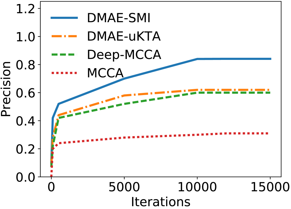
(a) Precision.

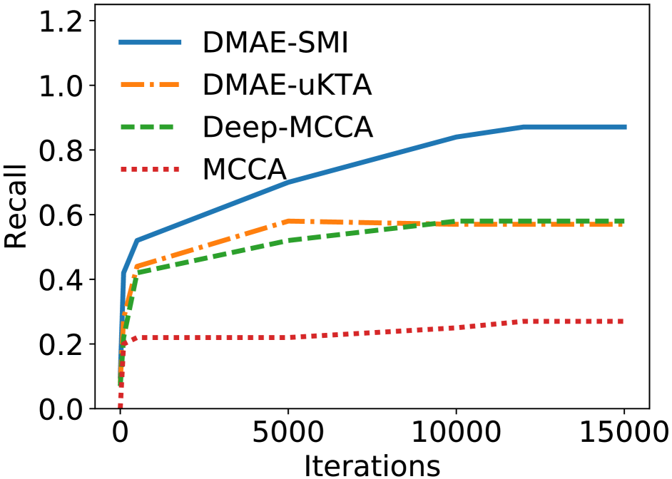
(b) Recall.

Figure 3: Evolution of ${\bm{\Pi}}$ (label) matrix prediction accuracy during unsupervised classifier learning.

Results: Testing Accuracy  To complete the evaluation of the actual learned classifier, we next assume that the estimated $\widehat{{\bm{\Pi}}}$ label matrix is correct, and use these labels to train a SVM classifier, which is evaluated on the testing split of each dataset. The results for CIFAR-10 and AwA are shown in Tables 3 and 4 respectively. As shown by the L/U/T proportions listed, supervised (all training data pairs given), semi-supervised (some training pairs given), semi-supervised transductive, and unsupervised (no training pairs given) settings are evaluated. From the results we can see that: (i) Our unsupervised learned classifiers work well (eg DMAE-SMI in 0-40-60 condition on AwA is 32% vs 2% chance). (ii) Our method can exploit semi-supervised learning (eg in CIFAR the 10-40-10 vs 10-0-10 condition shows the benefit of exploiting 80% unlabeled train data in addition to 20% labeled train data). (iii) We can also exploit seamlessly semi-supervised transductive learning if unpaired testing data is available (top vanilla vs bottom transductive condition). (iv) Our method outperforms alternatives in each experiment (DMAE-SMI vs others).

Table 3: Classification accuracy on CIFAR-10 test set. The data is split into labeled training data (L), unlabeled training data (U) and test data (T) in units of 10,000. Train on L and U, test on T.

CIFAR-10
L-U-T data (10K)	DMAE-SMI	DMAE-uKTA	Deep-MCCA	MCCA
0-50-10	0.70	0.59	0.20	0.15
10-40-10	0.86	0.73	0.40	0.26
10- 0-10	0.72	0.62	0.21	0.17
50- 0-10	0.91	0.84	0.57	0.52
CIFAR-10 Transductive
0-50-10	0.76	0.66	0.22	0.16
10-40-10	0.89	0.80	0.45	0.29
10- 0-10	0.75	0.64	0.23	0.16
50- 0-10	0.92	0.85	0.60	0.54

Table 4: Classification accuracy on AWA test set (50-way). The data is split into labeled training data (L), unlabeled training data (U) and test data (T) with listed %. Train on L and U, test on T.

AwA
L-U-T data (%)	DMAE-SMI	DMAE-uKTA	Deep-MCCA	MCCA
0-40-60	0.32	0.20	0.16	0.12
20- 0-60	0.40	0.28	0.15	0.11
20-20-60	0.47	0.32	0.18	0.14
40- 0-60	0.60	0.48	0.24	0.18
AWA Transductive
0-40-60	0.42	0.28	0.21	0.16
20-20-60	0.54	0.40	0.22	0.17
20- 0-60	0.52	0.38	0.22	0.17
40- 0-60	0.70	0.52	0.28	0.20

5 Conclusion

We proposed Deep Matching Autoencoders (DMAE), which are capable of learning pairing and a common latent space from unpaired multi-modal. The  DMAE  approach elegantly spans unsupervised, semi-supervised, fully supervised and zero-shot settings. In the supervised setting it is competitive with state of the art alternatives on captioning. In the less studied semi-supervised and unsupervised settings it outperforms the few existing alternatives. Prior studies of unsupervised cross-domain matching have generally used toy data. We showed that our DMAE approach can scale to real vision and language data and solve a novel unsupervised classifier learning problem. Although we evaluated our approach on captioning and classifier learning, it is a widely applicable cross-modal method with potential applications from person re-identification [11] to word-alignment [7], which we will explore in future work.

References

- [1] S. M. Ali and S. D. Silvey. A general class of coefficients of divergence of one distribution from another. Journal of the Royal Statistical Society. Series B (Methodological), 28(1):131–142, 1966.
- [2] G. Andrew, R. Arora, J. Bilmes, and K. Livescu. Deep canonical correlation analysis. In ICML, 2013.
- [3] F. R. Bach and M. I. Jordan. Kernel independent component analysis. JMLR, 3:1–48, Mar. 2003.
- [4] S. Chandar, M. M. Khapra, H. Larochelle, and B. Ravindran. Correlational neural networks. Neural Computation, 28(2):257–285, February 2016.
- [5] B. Chang, U. Kruger, R. Kustra, and J. Zhang. Canonical correlation analysis based on hilbert-schmidt independence criterion and centered kernel target alignment. In ICML, 2013.
- [6] A. Coates and A. Y. Ng. The importance of encoding versus training with sparse coding and vector quantization. In ICML, 2011.
- [7] A. Conneau, G. Lample, M. Ranzato, L. Denoyer, and H. Jégou. Word translation without parallel data. CoRR, abs/1710.04087, 2017.
- [8] B. Coyne and R. Sproat. Wordseye: An automatic text-to-scene conversion system. In SIGGRAPH, 2001.
- [9] N. Cristianini, J. Shawe-Taylor, A. Elisseeff, and J. S. Kandola. On kernel-target alignment. In NIPS, 2002.
- [10] N. Djuric, M. Grbovic, and S. Vucetic. Convex kernelized sorting. In AAAI, 2012.
- [11] F. Feng, X. Wang, and R. Li. Cross-modal retrieval with correspondence autoencoder. In ACM Multimedia, 2014.
- [12] A. Frome, G. Corrado, J. Shlens, S. Bengio, J. Dean, M. Ranzato, and T. Mikolov. Devise: A deep visual-semantic embedding model. In NIPS, 2013.
- [13] K. P. F.R.S. X. on the criterion that a given system of deviations from the probable in the case of a correlated system of variables is such that it can be reasonably supposed to have arisen from random sampling. The London, Edinburgh, and Dublin Philosophical Magazine and Journal of Science, 50(302):157–175, 1900.
- [14] Y. Fu, T. Hospedales, T. Xiang, and S. Gong. Transductive multi-view zero-shot learning. IEEE TPAMI, 37(11):2332 – 2345, 2015.
- [15] S. Gong, M. Cristani, S. Yan, and C. C. Loy, editors. Person Re-Identification. Springer, 2014.
- [16] Y. Gong, Q. Ke, M. Isard, and S. Lazebnik. A multi-view embedding space for modeling internet images, tags, and their semantics. IJCV, 2013.
- [17] A. Gretton, O. Bousquet, A. Smola, and B. Schölkopf. Measuring statistical dependence with Hilbert-schmidt norms. In ALT, 2005.
- [18] S. Guadarrama, N. Krishnamoorthy, G. Malkarnenkar, S. Venugopalan, R. Mooney, T. Darrell, and K. Saenko. YouTube2Text: Recognizing and describing arbitrary activities using semantic hierarchies and zero-shot recognition. In ICCV, 2013.
- [19] A. Gupta, Y. Verma, and C. V. Jawahar. Choosing linguistics over vision to describe images. In AAAI, 2012.
- [20] A. Haghighi, P. Liang, T. Berg-Kirkpatrick, and D. Klein. Learning bilingual lexicons from monolingual corpora. In ACL, 2008.
- [21] D. R. Hardoon, S. R. Szedmak, and J. R. Shawe-taylor. Canonical correlation analysis: An overview with application to learning methods. Neural Computation, 16(12):2639–2664, 2004.
- [22] S. Hochreiter and J. Schmidhuber. Long short-term memory. Neural Computation, 9(8):1735–1780, 1997.
- [23] H. Hotelling. Relations between two sets of variates. Biometrika, 28(3/4):321–377, 1936.
- [24] T. Iwata, T. Hirao, and N. Ueda. Unsupervised cluster matching via probabilistic latent variable models. In AAAI, 2013.
- [25] J. Jagarlamudi, S. Juarez, and H. Daumé III. Kernelized sorting for natural language processing. In AAAI, 2010.
- [26] T. Jebara. Kernelizing sorting, permutation and alignment for minimum volume PCA. In Conference on Learning Theory, 2004.
- [27] M. Kan, S. Shan, and X. Chen. Multi-view deep network for cross-view classification. In CVPR, 2016.
- [28] A. Karpathy and L. Fei-Fei. Deep visual-semantic alignments for generating image descriptions. IEEE TPAMI, 39(4):664–676, 2017.
- [29] B. Klein, G. Lev, G. Sadeh, and L. Wolf. Associating neural word embeddings with deep image representations using fisher vectors. In CVPR, 2015.
- [30] N. Krishnamoorthy, G. Malkarnenkar, R. Mooney, K. Saenko, and S. Guadarrama. Generating natural-language video descriptions using text-mined knowledge. In AAAI, 2013.
- [31] A. Krizhevsky and G. Hinton. Learning multiple layers of features from tiny images. 2009.
- [32] C. H. Lampert, H. Nickisch, and S. Harmeling. Learning to detect unseen object classes by between-class attribute transfer. In CVPR, 2009.
- [33] C. H. Lampert, H. Nickisch, and S. Harmeling. Attribute-based classification for zero-shot visual object categorization. IEEE TPAMI, 36(3):453–465, 2014.
- [34] T.-Y. Lin, M. Maire, S. Belongie, J. Hays, P. Perona, D. Ramanan, P. Dollár, and C. L. Zitnick. Microsoft COCO: Common Objects in Context. 2014.
- [35] T. Mikolov, I. Sutskever, K. Chen, G. S. Corrado, and J. Dean. Distributed representations of words and phrases and their compositionality. In NIPS, 2013.
- [36] J. Ngiam, A. Khosla, M. Kim, J. Nam, H. Lee, and A. Y. Ng. Multimodal deep learning. In ICML, 2011.
- [37] V. Ordonez, G. Kulkarni, and T. L. Berg. Im2text: Describing images using 1 million captioned photographs. In NIPS, 2011.
- [38] S. Ouyang, T. Hospedales, Y.-Z. Song, X. Li, C. C. Loy, and X. Wang. A survey on heterogeneous face recognition: Sketch, infra-red, 3d and low-resolution. Image and Vision Computing, 56:28 – 48, 2016.
- [39] N. Quadrianto, L. Song, and A. J. Smola. Kernelized sorting. In NIPS, 2009.
- [40] K. Simonyan and A. Zisserman. Very deep convolutional networks for large-scale image recognition. arXiv preprint arXiv:1409.1556, 2014.
- [41] R. Socher, M. Ganjoo, C. D. Manning, and A. Y. Ng. Zero-shot learning through cross-modal transfer. In NIPS, 2013.
- [42] T. Suzuki and M. Sugiyama. Sufficient dimension reduction via squared-loss mutual information estimation. In AISTATS, 2010.
- [43] Y. H. Tsai, L. Huang, and R. Salakhutdinov. Learning robust visual-semantic embeddings. In ICCV, 2017.
- [44] L. Wang, Y. Li, and S. Lazebnik. Learning deep structure-preserving image-text embeddings. In CVPR, 2016.
- [45] L. Wang, Y. Li, and S. Lazebnik. Learning two-branch neural networks for image-text matching tasks. CoRR, abs/1704.03470, 2017.
- [46] M. Yamada, L. Sigal, M. Raptis, M. Toyoda, Y. Chang, and M. Sugiyama. Cross-domain matching with squared-loss mutual information. IEEE TPAMI, 37(9):1764–1776, 2015.
- [47] M. Yamada and M. Sugiyama. Cross-domain object matching with model selection. In AISTATS, 2011.
- [48] F. Yan and K. Mikolajczyk. Deep correlation for matching images and text. In CVPR, 2015.
- [49] P. Young, A. Lai, M. Hodosh, and J. Hockenmaier. From image descriptions to visual denotations: New similarity metrics for semantic inference over event descriptions. TACL, 2:67–78, 2014.