Frame Interpolation with Multi-Scale Deep Loss Functions and Generative Adversarial Networks

Abstract

Frame interpolation attempts to synthesise frames given one or more consecutive video frames. In recent years, deep learning approaches, and notably convolutional neural networks, have succeeded at tackling low- and high-level computer vision problems including frame interpolation. These techniques often tackle two problems, namely algorithm efficiency and reconstruction quality. In this paper, we present a multi-scale generative adversarial network for frame interpolation (FIGAN). To maximise the efficiency of our network, we propose a novel multi-scale residual estimation module where the predicted flow and synthesised frame are constructed in a coarse-to-fine fashion. To improve the quality of synthesised intermediate video frames, our network is jointly supervised at different levels with a perceptual loss function that consists of an adversarial and two content losses. We evaluate the proposed approach using a collection of 60fps videos from YouTube-8m. Our results improve the state-of-the-art accuracy and provide subjective visual quality comparable to the best performing interpolation method at $\times 47$ faster runtime.

1 Introduction

Frame interpolation attempts to synthetically generate one or more intermediate video frames from existing ones, the simple case being the interpolation of one frame given two adjacent video frames. This is a challenging problem requiring a solution that can model natural motion within a video, and generate frames that respect this modelling. Artificially increasing the frame-rate of videos enables a range of applications. For example, data compression can be achieved by actively dropping video frames at the emitting end and recovering them via interpolation on the receiving end [1]. Increasing video frame-rate also directly allows to improve visual quality or to obtain an artificial slow-motion effect [2, 3, 4].

(a) Original image

(b) Original

(c) [5]

(d) [6]

(e) FIGAN

Figure 1: Visual example of frame interpolation results using PCA-layers [5], SepConv $\mathcal{L}_{F}$ [6], and the proposed solution FIGAN, which combines a multi-scale neural network design with a perceptual training loss that surpasses state-of-the-art accuracy with real-time runtime. Visual quality is comparable to SepConv [6] while requiring $\times 3.24$ fewer computations.

Frame interpolation commonly relies on optical flow [7, 8, 9, 4]. Optical flow relates consecutive frames in a sequence describing the displacement that each pixel undergoes from one frame to the next. One solution for frame interpolation is therefore to assume constant velocity in motion between existing frames and interpolate frames via warping. However, optical flow estimation is difficult and time-consuming, and a good illustration of this is that the average run-time per $480\times 640$ frame of the top five performing methods of 2017 in the Middlebury benchmark dataset [9] is 1.47 minutes. Furthermore, there is in general no consensus on a single model that can accurately describe it. Different models have been proposed based on inter-frame colour or gradient constancy, but these are susceptible to failure in challenging conditions such as occlusion, illumination or nonlinear structural changes. As a result, methods that obtain frame interpolation as a derivative of flow suffer from inaccuracies in flow estimation.

Recently, deep learning approaches, and in particular Convolutional Neural Networks (CNNs), have set up new state-of-the-art results across many computer vision problems, and have also provided new optical flow estimation methods. In [10, 11], optical flow features are trained in a supervised setup mapping two frames to their ground truth optical flow field. Spatial transformer networks [12] allow an image to be spatially transformed as part of a differentiable network, learning a transformation implicitly in an unsupervised fashion, hence enabling frame interpolation with an end-to-end differentiable network [4]. Choices in network design and training strategy can directly affect interpolation quality as well as efficiency. Multi-scale residual estimations have been repeatedly proposed in the literature [13, 14, 8], but only simple models based on colour constancy have been explored. More recently, training strategies have been proposed for low-level vision tasks to go beyond pixel-wise error metrics making use of more abstract data representations and adversarial training, producing visually more pleasing results [15, 16]. An example of this notion applied to frame interpolation networks is explored very recently in [6].

In this paper we propose a real-time frame interpolation method that can generate realistic intermediate frames with high Peak Signal-to-Noise Ratio (PSNR). It is the first model that combines the pyramidal structure of classical optical flow modeling with recent advances in spatial transformer networks for frame interpolation. Compared to naive CNN processing, this leads to a $\times 9,3$ speedup with a $2.38$dB increase in PSNR. Furthermore, to work around natural limitations of intensity variations and nonlinear deformations, we investigate deep loss functions and adversarial training. These contributions result in an interpolation model that is more expressive and informative relative to models based solely on pixel intensity losses as illustrated in Table 3 and Fig. 6.

2 Related Work

2.1 Frame interpolation with optical flow

The main challenge in frame interpolation lies in respecting object motion and occlusions such as to recreate a plausible frame that preserves structure and consistency of data. Although there has been work in frame interpolation without explicit motion estimation [3], the vast majority of methods relies on flow estimation as a description of motion across frames [9, 8, 4].

Let us define two consecutive frames with $I_{0}$ and $I_{1}$, their optical flow relationship can be formulated as

$$I_{0}(x,y)=I_{1}(x+u,y+v),$$ (1)

where $u$, and $v$ are pixel-wise displacement fields for dimensions $x$ and $y$. For convenience, we will use the shorter notation $I(\Delta)$ to refer to an image $I$ with coordinate displacement $\Delta=(u,v)$, and write $I_{0}=I_{1}(\Delta)$. Multiple strategies can be adopted for the estimation of $\Delta$, ranging from a classic minimisation of an energy functional given flow smoothness constraints [17], to recent proposals employing neural networks [10]. Flow amplitude can vary greatly (eg. slow moving details versus camera panning), and in order to efficiently account for this variability flow can be approximated at multiple scales. Finer flow scales take advantage of estimations at lower coarse scales to progressively estimate the final flow in a coarse-to-fine fashion [18, 19, 20]. Given an optical flow between two frames, an interpolated intermediate frame $\hat{I}_{0.5}$ can be estimated by projecting the flow at time $t=0.5$ and pulling intensity values bidirectionally from frames $I_{0}$ and $I_{1}$. A description of this interpolation mechanism can be found in [9].

2.2 Neural networks for frame interpolation

Neural network solutions have been proposed for the supervised learning of optical flow fields from labelled data [10, 11, 21, 6]. Although these have been successful and could be used for frame interpolation in the paradigm of flow estimation and independent interpolation, there exists an inherent limitation in that flow labelled data is scarce and expensive to produce. It is possible to work around this limitation by training on rendered videos where ground truth flow is known [10, 11], although this solution is susceptible to overfitting synthetically generated data. An approach to directly interpolate images has been recently suggested in [21, 6] where large convolution kernels are estimated for each output pixel value. Although results are visually appealing, the complexity of these approaches has not been constrained to meet real-time runtime requirements.

Spatial transformers [12] have recently been used for unsupervised learning of optical flow by learning how to warp a video frame onto its consecutive frame [22, 23, 24]. In [4] it is used to directly synthesise an interpolated frame using a CNN to estimate flow features and spatial weights to handle occlusions. Although flow is estimated at different scales, fine flow estimations do not reuse coarse flow estimation like in the traditional pyramidal flow estimation paradigm, potentially indicating design inefficiencies.

2.3 Deep loss functions

Low-level vision problem optimisation often minimise a pixel-wise metric such as squared or absolute errors, as these are objective definitions of the distance between true data and its estimation. However, it has been recently shown how departing from pixel space to evaluate modelling error in a different, more abstract dimensional space can be beneficial. In [15] it is shown how high dimensional features from the VGG network are helpful in constructing a training loss function that correlates better with human perception than Mean-Squared Error (MSE) for the task of image super-resolution. In [16] this is further enhanced with the use of Generative Adversarial Networkss (GANs). Neural network solutions for frame interpolation have been limited to the choice of classical objective metrics such as colour constancy [4, 21], but recently [6] has shown how perceptual losses can also be beneficial for this problem. Training for frame interpolation involving adversarial losses have nevertheless not yet been explored.

2.4 Contribution

We propose a neural network solution for frame interpolation that benefits from a multi-scale refinement of the flow learnt implicitly. The structural change to progressively apply and estimate flow fields has runtime implications as it presents an efficient use of computational network resources compared to the baseline as illustrated in Table 2. Additionally, we introduce a synthesis refinement module for the interpolation result inspired by [25], which shows helpful in correcting reconstruction results. Finally, we propose a higher level, more expressive interpolation error modelling taking account of classical colour constancy, a perceptual loss and an adversarial loss functions. Our main contributions are:

• A real-time neural network for frame interpolation.

• A multi-scale network architecture inspired by multi-scale optical flow estimation that progressively applies and refines flow fields.

• A reconstruction network module that refines frame synthesis results.

• A training loss function that combines colour constancy, a perceptual and adversarial losses.

3 Proposed Approach

The method proposed is based on a trainable CNN architecture that directly estimates an interpolated frame from two input frames $I_{0}$ and $I_{1}$. This approach is similar to the one in [4], where given many examples of triplets of consecutive frames, we solve an optimisation task minimising a loss between the estimated frame $\hat{I}_{0.5}$ and the ground truth intermediate frame $I_{0.5}$. A high-level overview of the method is illustrated in Fig. 2, and details about it’s design and training are detailed in the following sections.

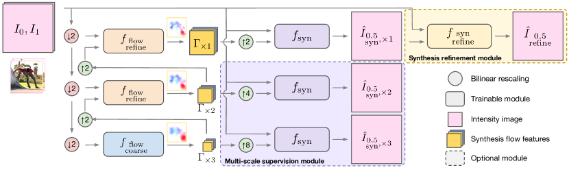
Figure 2: Overview of the frame interpolation method. Flow is estimated from two input frames at scales $\times 8$, $\times 4$ and $\times 2$. The finest flow scale is used to synthesise the final frame. Optionally, intermediate flow scales can be used to synthesise coarse interpolated frames in a multi-scale supervision module contributing to the training cost function, and the synthesised frame can be further processed through a synthesis refinement module.

3.1 Network design

3.1.1 Multi-scale frame synthesis

Let us assume $\Delta$ to represent the flow from time point $0.5$ to $1$, and for convenience, let us refer to synthesis features as $\Gamma=\{\Delta,W\}$, where spatial weights $W_{i,j}=[0,1]\;\forall i,j$ can be used to handle occlusions and disocclusions. The synthesis interpolated frame is then given by

$$\hat{I}_{\begin{subarray}{c}0.5\\ \text{syn}\end{subarray}}=f_{\text{syn}}(I_{0},I_{1},\Gamma)=W\circ I_{0}(-\Delta)+(1-W)\circ I_{1}(\Delta),$$ (2)

with $\circ$ denoting the Hadamard product. This is used in [4] to synthesise the final interpolated frame and is referred to as voxel flow. Although a multi-scale estimation of synthesis features $\Gamma$ is presented to process input data at different scales, coarser flow levels are not leveraged for the estimation of finer flow results. In contrast, we propose to reuse a coarse flow estimation for further processing with residual modules, in the same spirit as in [25].

To estimate synthesis features $\Gamma$ we build a pyramidal structure progressively applying and estimating optical flow between two frames at different scales $j=[1,J]$, with $J$ the coarsest level. We refer to synthesis features at different scales as $\Gamma_{\times j}$. If $U$ and $D$ denote $\times 2$ bilinear up- and down-sampling matrix operators, flow features are obtained as

$$\Gamma_{\times j}=\begin{cases}f_{\begin{subarray}{c}\text{flow}\\ \text{coarse}\end{subarray}}(D^{j}I_{0},D^{j}I_{1})&\text{if $j=J$},\\ f_{\begin{subarray}{c}\text{flow}\\ \text{refine}\end{subarray}}(D^{j}I_{0},D^{j}I_{1},U\Gamma_{\times(j+1)})&\text{otherwise}.\end{cases}$$ (3)

The processing for flow refinement is show in Fig. 3, and is formally given by

$$f_{\begin{subarray}{c}\text{flow}\\ \text{refine}\end{subarray}}(I_{0},I_{1},\Gamma)=\text{tanh}(\Gamma+\Gamma_{\text{res}}),$$ (4)

$$\Gamma_{\text{res}}=f_{\begin{subarray}{c}\text{flow}\\ \text{res}\end{subarray}}(I_{0}(-\Delta),I_{1}(\Delta),\Gamma),$$ (5)

with the tanh non-linearity keeping the synthesis flow features within the range $[-1,1]$. The coarse flow estimation and flow residual modules, $f_{\begin{subarray}{c}\text{flow}\\ \text{coarse}\end{subarray}}$ and $f_{\begin{subarray}{c}\text{flow}\\ \text{res}\end{subarray}}$ in Fig. 2 and Fig. 3 respectively, are both based on the CNN architecture described in Table 1. Both modules use $\phi=\text{tanh}$ to produce $N_{o}=3$ output synthesis features within the range $[-1,1]$, corresponding to flow features $\Gamma$. For $3$ image color channels, coarse flow estimation uses $N_{i}=6$, and residual flow uses $N_{i}=9$.

Fixing $J=3$, found to be a good compromise between efficiency and performance, the final features are upsampled from the first scale to be $\Gamma=U\Gamma_{\times 1}$. Note that intermediate synthesis features can be used to obtain intermediate synthesis results as

$$\hat{I}_{\begin{subarray}{c}0.5\\ \text{syn}\end{subarray},\times j}=f_{\text{syn}}(I_{0},I_{1},U^{j}\Gamma_{\times j}).$$ (6)

In Section 3.2.1 we describe how intermediate synthesis results can be used in a multi-scale supervision module to facilitate network training.

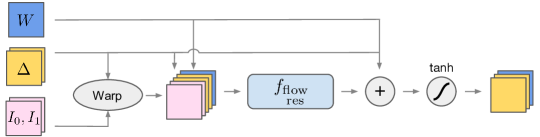
Figure 3: Flow refinement module. A coarse flow estimation wraps the input frames, which are then passed together with the coarse synthesis flow features to a flow residual module. The sum of the residual flow and the coarse flow features results in a fine flow estimation . A tanh non-linearity clips the result to within $[-1,1]$.

3.1.2 Synthesis refinement module

Frame synthesis can be challenging in cases of complex motion or occlusions where flow estimation may be inaccurate. In these situations, artifacts usually produce an unnatural look for moving regions of the image that benefit from further correction. We therefore introduce a synthesis refinement module that consists of a CNN allowing for further joint processing of the synthesised image with the original input frames that produced it.

$$\hat{I}_{\begin{subarray}{c}0.5\\ \text{refine}\end{subarray}}=f_{\begin{subarray}{c}\text{syn}\\ \text{refine}\end{subarray}}(\hat{I}_{\begin{subarray}{c}0.5\\ \text{syn}\end{subarray}},I_{0},I_{1}).$$ (7)

This was shown in [25] to be beneficial in refining the brightness of a reconstruction result and to handle difficult occlusions. This module also uses the convolutional block in Table 1 with $N_{i}=9$, $N_{o}=3$ and $\phi$ the identity function.

Layer	Convolution kernel	Non-linearity
$1$	$N_{i}\times 32\times 3\times 3$	ReLU
$2$, …, $5$	$32\times 32\times 3\times 3$	ReLU
$6$	$32\times N_{o}\times 3\times 3$	$\phi$

Table 1: Convolutional network block used for coarse flow, flow residual and reconstruction refinement modules. Convolution kernels correspond to number of input and output features, followed by kernel size dimensions $3\times 3$.

3.2 Network training

Given loss functions $l_{i}$ between the network output and the ground-truth frame, defined for an arbitrary number of components $i=\{1,I\}$, we solve

$$\hat{I}_{0.5}=\operatorname*{arg\,min}_{\theta}\frac{1}{N}\sum_{n=1}^{N}\sum_{i=1}^{I}\lambda_{i}l_{i}\left(f_{\theta}(I^{n}_{0},I^{n}_{1}),I^{n}_{0.5}\right).$$ (8)

The output $\hat{I}_{0.5}$ is $\hat{I}_{\begin{subarray}{c}0.5\\ \text{syn}\end{subarray}}$ or $\hat{I}_{\begin{subarray}{c}0.5\\ \text{refine}\end{subarray}}$ depending on whether the refinement module is used, and $\theta$ represents all trainable parameters in the interpolation network $f_{\theta}$.

3.2.1 Multi-scale synthesis supervision

The multi-scale frame synthesis described in Section 3.1.1 can be used to define a loss function at the finest synthesis scale with a synthesis loss

$$l_{\text{syn},\times 1}=\tau(\hat{I}_{\begin{subarray}{c}0.5\\ \text{syn}\end{subarray},\times 1},I_{0.5}),$$ (9)

with $\tau$ a distance metric. However, an optimisation task based solely on this cost function suffers from the fact that it leads to an ill-posed solution, that is, for one particular flow map there will be multiple possible solutions. It is therefore likely that the solution space contains many local minima, making it challenging to solve via gradient descent. The network can for instance easily get stuck in degenerate solutions where a case with no motion, $\Gamma_{\times 1}=\mathbf{0}$, is represented by the network as $\Gamma_{\times 1}=U\Gamma_{\times 2}+U^{2}\Gamma_{\times 3}$, in which case there are infinite solutions for the flow fields at each scale.

In order to prevent this, we supervise the solution of all scales such that flow estimation is required to be accurate at all scales. In practice, we define the following multi-scale synthesis loss function

$$l_{\begin{subarray}{c}\text{multi}\\ \text{syn}\end{subarray}}=\sum_{j=1}^{J}\lambda_{\text{syn},j}l_{\text{syn},\times j}.$$ (10)

We heuristically choose the weighting of this multiscale loss to be $\lambda_{\text{syn},j}=\{1\text{ if }j=1;0.5\text{ otherwise}\}$ to prioritise the synthesis at the finest scale.

Additionally, the network using the synthesis refinement module adds a term to the cost function expressed as

$$l_{\begin{subarray}{c}\text{syn}\\ \text{refine}\end{subarray}}=\tau(\hat{I}_{\begin{subarray}{c}0.5\\ \text{refine}\end{subarray}},I_{0.5}),$$ (11)

and the total loss function for $J=3$ scales is

$$L=l_{\begin{subarray}{c}\text{multi}\\ \text{syn}\end{subarray}}+l_{\begin{subarray}{c}\text{syn}\\ \text{refine}\end{subarray}}=l_{\text{syn},\times 1}+\frac{1}{2}[l_{\text{syn},\times 2}+l_{\text{syn},\times 3}]+l_{\begin{subarray}{c}\text{syn}\\ \text{refine}\end{subarray}}.$$ (12)

We propose to combine traditional pixel-wise distance metrics with higher order metrics given by a deep network, which have been shown to correlate better with human perception. As a pixel-wise metric we choose the $l1$-norm, which has been shown to produce sharper interpolation results than MSE [26], and we employ features 5_4 from the VGG network [27] as a perceptual loss, as proposed in [15, 16]. Denoting with $\gamma$ the transformation of an image to VGG space, the distance metric is therefore given by

$$\tau(a,b)=\|a-b\|_{1}+\lambda_{\text{VGG}}\|\gamma(a)-\gamma(b)\|^{2}_{2}.$$ (13)

Throughout this work we fix $\lambda_{\text{VGG}}=0.001$. We include results when this term is not included in training ($\lambda_{\text{VGG}}=0$) to analyse its impact.

3.2.2 Generative adversarial training

In the loss functions described above, there is no mechanism to avoid solutions that may not be visually pleasing. A successful approach to force the solution manifold to correspond with images of a realistic appearance has been GAN training. We can incorporate such loss term to the objective function Eq. 12 as follows

$$L=l_{\begin{subarray}{c}\text{multi}\\ \text{syn}\end{subarray}}+l_{\begin{subarray}{c}\text{syn}\\ \text{refine}\end{subarray}}+0.0001l_{\text{GAN}}$$ (14)

Let us call the interpolation network the generator network $f_{\theta_{G}}$, the GAN term $l_{\text{GAN}}$ optimises the loss function

$$\min_{\theta_{G}}\max_{\theta_{D}} \mathbb{E}_{I_{0.5}\sim p_{\text{train}}(I_{0.5})}[\log d_{\theta_{D}}(I_{0.5})]+$$ (15)

$$\mathbb{E}_{(I_{0},I_{1})\sim p_{f}(I_{0},I_{1})}[\log(1-d_{\theta_{D}}(f_{\theta_{G}}(I_{0},I_{1}))))],$$ (16)

with $d_{\theta_{D}}$ representing a discriminator network that tries to discriminate original frames from interpolated results. The weighting parameter $0.0001$ was chosen heuristically in order to avoid the GAN loss overwhelming the total loss.

Adding this objective to the loss forces the generator $f_{\theta_{G}}$ to attempt fooling the discriminator. It has been shown that in practice this leads to image reconstructions that incorporate visual properties of photo-realistic images, such as improved sharpness and textures [16, 28]. The discriminator architecture is based on the one described in figure 4 of [16], with minor modifications. We start with 32 filters and follow up with 8 blocks of convolution, batch normalization and leaky ReLU with alternating strides of 2 and 1. At each block of stride 2 the number of features is doubled, which we found to improve the performance of the discriminator.

4 Experiments

We first compute the performance of a baseline version of the model that performs single-scale frame synthesis without synthesis refinement and is trained using a simple colour constancy $l1$-norm loss. We gradually incorporate to a baseline network the design and training choices proposed in Section 3.1 and Section 3.2, and evaluate their benefits visually and quantitatively. As a performance metric for reconstruction accuracy we use PSNR, however we note that this metric is known to not correlate well with human perception [16].

4.1 Data and implementation details

The dataset used is a collection of 60fps videos from YouTube-8m [29] resized to $640\times 360$. Training samples are obtained by extracting one triplet of consecutive frames every second, discarding samples for which two consecutive frames were found to be almost identical with a small squared error threshold. Unless otherwise stated, all models used $20$k, $1.5$k and $375$ triplets of frames corresponding to the training, validation and testing sets.

All network layers from convolutional building blocks based on Table 1 are orthogonally initialised with a gain of $\sqrt{2}$, except for the final layer which is initialised from a normal distribution with standard deviation $0.01$. This forces the network to initialise flow estimation close to zero, which leads to more stable training. Training was performed on batches of size $128$ using frame crops of size $128\times 128$ to diversify the content of batches and increase convergence speed. Furthermore, we used Adam optimisation [30] with learning rate $0.0001$ and applied early stopping with a patience of 10 epochs. All models converge around roughly $100$ epochs with this setup.

4.2 Complexity and speed analysis

To remain framework and hardware agnostic, we report computational complexity of CNNs in floating point operations (FLOPs) necessary for the processing of one $360\times 640$ frame, and in the number of trainable parameters. The bottleneck of the computation is in convolutional operations to estimate a flow field and refine the interpolation, therefore we ignore operations necessary for intermediate warping stages. Using $H$ and $W$ to denote height and width, $n_{l}$ the number of features in layer $l$, and $k$ the kernel size, the number of FLOPs per convolution are approximated as

$$HWn_{l+1}\left[2n_{l}k^{2}+2\right].$$ (17)

We additionally report GPU runtimes for the methods proposed as well as for SepConv $\mathcal{L}_{F}$ as a reference for network efficiency. Experiments were run on an NVIDIA M40 GPU.

4.3 Network design experiments

In the first set of experiments we evaluate the benefits of exploiting an implicit estimation of optical flow as well as a synthesis refinement module.

4.3.1 Implicit optical flow estimation

CNNs can spatially transform information through convolutions without the need for spatial transformer pixel regridding. However, computing an internal representation of optical flow that is used by a transformer is a more efficient alternative to achieve this goal. In Table 2 we compare results for our baseline architecture using multi-scale synthesis (MS $l_{\text{syn},\times 1}$), relative to a simple CNN that attempts to directly estimate frame $I_{0.5}$ from inputs $I_{0}$ and $I_{1}$. Both models are trained with $l1$-norm colour constancy loss (ie. $\lambda_{\text{VGG}}=0$ in Eq. 13). In order to replicate hyperparameters, all layers in the baseline CNN model are convolutional layers of $32$ kernels of size $3\times 3$ followed by ReLU activations, except for the last layer which uses a linear activation.

The baseline model uses $15$ layers, which results in approximately the same number of trainable parameters to the proposed spatial transformer method. Note that the multi-scale design allows to obtain an estimation with $\times 9.2$ fewer FLOPs. The baseline CNN produces a PSNR $2.4$dB lower than multi-scale synthesis on the test set. The visualisations in Fig. 4 show that the baseline CNN struggles to produce a satisfactory interpolation (b, d), and tends to produce an average of previous and past frames. The proposed multi-scale synthesis method results in more accurate approximations (e, g).

Method	PSNR	Parameters	FLOPs
Baseline CNN	$33.93$	$123$k	$57$G
MS $l_{\text{syn},\times 1}$	$36.31$	$121$k	$6.1$G
MS $l_{\text{syn},\times 1}+l_{\text{refine}}$	$36.78$	$161$k	$25$G

Table 2: Impact of network design on performance.

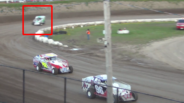
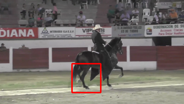
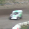
(a)

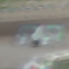
(b)

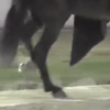
(c)

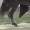
(d)

(e)

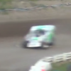
(f)

(g)

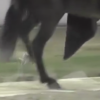
(h)

Figure 4: Impact of network design on two visual examples. Top: two full size original $360\times 640$ images with highlighted crops. Bottom: (a, c) ground-truth, (b, d) baseline CNN, (e, g) MS $l_{\text{syn},\times 1}$, (f, h) MS $l_{\text{syn},\times 1}+l_{\text{refine}}$.

4.3.2 Synthesis refinement

Frames directly synthesised from flow estimation can exhibit spatial distortions leading to visually unsatisfying results. This limitation can be substantially alleviated with the refinement module described in Section 3.1.2. In Table 2 we also include results for a multi-scale synthesis model that additionally uses a synthesis refinement module (MS $l_{\text{syn},\times 1}+l_{\text{refine}}$). This increases the number of trainable parameters by $\times 1.33$ and the number of FLOP by $\times 4.1$, but achieves adds $0.47$dB in PSNR and is able to correct inaccuracies in the estimation from the simpler MS $l_{\text{syn},\times 1}$, as shown in Fig. 4 (f, h).

4.4 Network training experiments

In this section we analyse the impact on interpolation results brought by multi-scale synthesis supervision and by the use of a perceptual loss term and GAN training for an improved visual quality.

4.4.1 Multi-scale synthesis supervision

As described previously, the performance of synthesis models presented in Table 2 is limited by the fact that flow estimation in multiple scales is ill-posed. We retrained model MS $l_{\text{syn},\times 1}+l_{\text{refine}}$, showing the best performance from the design choices proposed, but changed the objective function to supervise frame interpolation at all scales as proposed in Section 3.2.1. This model, which we refer to as MS for brevity (short for MS $l_{\begin{subarray}{c}\text{multi}\\ \text{syn}\end{subarray}}+l_{\text{refine}}$), increases PSNR on the test set compared to MS $l_{\text{syn},\times 1}+l_{\text{refine}}$ by $0.19$dB up to $36.97$dB as shown in Table 3 when trained on the same set of $20$k training frames.

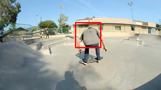
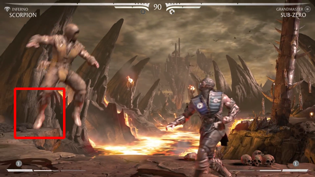
(a)

(b)

(c)

(d)

(e)

(f)

(g)

(h)

Figure 5: Impact of network training on two visual examples. Top: two full size original $360\times 640$ images with highlighted crops. Bottom: (a, c) ground-truth, (b, d) MS, (e, g) MS$+$VGG, (f, h) MS$+$VGG$+$GAN (FIGAN).

4.4.2 Impact of training data

Unsupervised motion learning is challenging due to the large space of possible video motion. In order to learn a generalisable representation of motion, it is important to have a diverse training set with enough representative examples of expected flow directions and amplitudes. We evaluated the same mode MS when trained on different training set sizes, in particular reducing the training set to $5$k random frames and increasing it to $200$k. Although increasing the training set size inevitably increases training time, it also has a considerable impact on PSNR as shown in Table 3. The remaining experiments use a training set size of $20$k as a compromise for performance and ease of experimentation.

4.4.3 Perceptual loss and GAN training

Extending the objective loss function with more abstract components such as a VGG term ($\lambda_{\text{VGG}}=0.001$ in Eq. 13) and a GAN training strategy (Eq. 14) also affects results. In Table 3 we also include results for a network MS$+$VGG, trained with the combination of $l1$-norm and VGG terms suggested in Eq. 13. We also show results for MS$+$VGG$+$GAN, which is a network additionally using adversarial training. This result of PSNR on the full test set shows that both of these modifications lower the performance relative to the simpler colour constancy training loss. However, a visual inspection of results in Fig. 5 demonstrate how these changes help obtaining a sharper, more pleasing interpolation. This is in line with the findings from [16, 6].

Method	Training set size	PSNR (dB)	FLOPs (G)	GPU speed (s)
Farneback [31]	-	$35.7$	-	-
Deep Flow 2 [14]	-	$35.88$	-	-
PCA-layers [5]	-	$36.3$	-	-
Phase-based [3]	-	$35.17$	-	-
FlowNet 2 [11]	-	$35.26$	-	-
SepConv $\mathcal{L}_{1}$ [6]	-	$37.04$	$81$	$0.7$
SepConv $\mathcal{L}_{F}$ [6]		$36.86$
MS	$5$k	$36.67$	$\mathbf{25}$	$\mathbf{0.015}$
	$20$k	$36.97$
	$200$k	$\mathbf{37.23}$
MS$+$VGG	$20$k	$36.89$	$\mathbf{25}$	$\mathbf{0.015}$
MS$+$VGG$+$GAN	$20$k	$36.68$	$\mathbf{25}$
(FIGAN)				$\mathbf{0.015}$

Table 3: State-of the-art interpolation comparison.

4.5 State-of-the-art comparison

In this section, several frame interpolation methods are compared to the algorithm proposed. Table 3 summarises PSNR results on the full tests set for all methods. The interpolation from flow-based methods [31, 14, 5, 11] was done as described in [9] using the optical flow features generated from implementations of the respective authors. The phase-based approach in [3] and SepConv [6] are both able to directly generate an interpolated frame. We include results from SepConv using both a colour constancy loss ($\mathcal{L}_{1}$) and a perceptual loss ($\mathcal{L}_{F}$).

As shown in Table 3, the best performing method in terms of PSNR is MS when trained on the large training set, however we found the best visual quality to be produced by FIGAN and SepConv-$\mathcal{L}_{F}$, both trained using perceptual losses. Visual examples from selected methods are provided in Fig. 6. Notice that some optical flow based methods such as Farneback and PCA-layers are unable to merge information from consecutive frames correctly, which can be attributed to an inaccurate flow estimation. In contrast, FIGAN shows more precise reconstructions, and most importantly preserves sharpness and features that make interpolation results perceptually more pleasing.

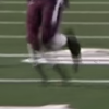
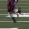
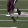
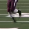
Figure 6: Visualisation of sate-of-the-art comparison. From left to right: full size original $360\times 640$ image with highlighted crop, Farneback’s method [31], PCA-layers [5], SepConv $\mathcal{L}_{F}$ [6], proposed FIGAN, and ground-truth.

(a) Original

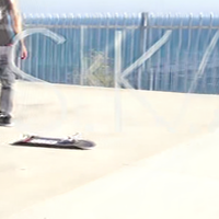
(b) SepConv $\mathcal{L}_{F}$

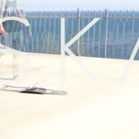
(c) FIGAN

Figure 7: SepConv $\mathcal{L}_{F}$ and FIGAN interpolation for conflicting overlaid motions. FIGAN favours an accurate reconstruction of the foreground while SepConv approximates the reconstruction of the background at the expense of distorting the foreground structure.

We found SepConv $\mathcal{L}_{F}$ and FIGAN to have visually comparable results for easily resolvable motion like those in Fig. 6. Their largest discrepancies in behaviour were found in challenging situations, such as static objects overlaid on top of a fast moving scene, as shown in Fig. 7. Whereas SepConv favours resolving large displacements in the background, FIGAN produces a better reconstruction of foreground objects at the expense of accuracy in the background. This could be due to the fact that SepConv estimates motion at $\times 32$ undersampling, while FIGAN only downscales by $\times 8$. Coarse-to-fine flow estimation approaches can fail when coarse scales dominate the motion of finer scales [32], and this is likely to be more pronounced the larger the gap between the coarse and fine scales.

A relevant difference between SepConv and FIGAN is found in complexity. SepConv includes $1.81$M training parameters, which is $\times 11.2$ more than FIGAN, but also each $360\times 640$ frame interpolation requires $81$G FLOPs, or $\times 3.24$ more compared to FIGAN. Noting a comparable visual quality and PSNR figures for a small fraction of training parameters, this highlights the efficiency advantages of FIGAN, which was designed under real-time constraints. The proposed networks run in real-time, attain state-of-the-art performance, and are $\times 47$ faster than the closest competing method.

5 Conclusion

In this paper, we have described a multi-scale network based on recent advances in spatial transformers and composite perceptual losses. Our proposed architecture sets a new state of the art in terms of PSNR, and produces visual quality results comparable to the best performing neural network solution with $\times 3.24$ fewer computations. Our experiments confirm that a network design drawing from traditional pyramidal flow refinement allows to reduce its complexity while maintaining a competitive performance. Furthermore, training losses beyond classical pixel-wise metrics and adversarial training provide an abstract representation that translate into sharper, and visually more pleasing interpolation results.

References

- [1] Sekiguchi, S., Idehara, Y., Sugimoto, K., Asai, K.: A low-cost video frame-rate up conversion using compressed-domain information. In: IEEE International Conference on Image Processing (ICIP). Volume 2. (2005) II–974
- [2] : RE: Vision Effects, Twixtor, accessed in Feb 2016 at http://revisionfx.com/products/twixtor/
- [3] Meyer, S., Wang, O., Zimmer, H., Grosse, M., Sorkine-Hornung, A.: Phase-based frame interpolation for video. In: IEEE Conference on Computer Vision and Pattern Recognition (CVPR). (2015) 1410–1418
- [4] Liu, Z., Yeh, R., Tang, X., Liu, Y., Agarwala, A.: Video frame synthesis using deep voxel flow. In: IEEE Intenational Conference on Computer Vision (ICCV). (2017)
- [5] Wulff, J., Black, M.J.: Efficient sparse-to-dense optical flow estimation using a learned basis and layers. In: IEEE Conference on Computer Vision and Pattern Recognition (CVPR). (2015) 120–130
- [6] Niklaus, S., Mai, L., Liu, F.: Video frame interpolation via adaptive separable convolution. In: IEEE International Conference on Computer Vision (ICCV). (2017)
- [7] Werlberger, M., Pock, T., Unger, M., Bischof, H.: Optical flow guided TV-L1 video interpolation and restoration. In: EMMCVPR, Springer (2011) 273–286
- [8] Rakêt, L.L., Roholm, L., Bruhn, A., Weickert, J.: Motion compensated frame interpolation with a symmetric optical flow constraint. In: International Symposium on Visual Computing, Springer (2012) 447–457
- [9] Baker, S., Scharstein, D., Lewis, J.P., Roth, S., Black, M.J., Szeliski, R.: A database and evaluation methodology for optical flow. International Journal of Computer Vision 92(1) (2011) 1–31
- [10] Dosovitskiy, A., Fischery, P., Ilg, E., Hazirbas, C., Golkov, V., van der Smagt, P., Cremers, D., Brox, T.: FlowNet: Learning optical flow with convolutional networks. In: IEEE International Conference on Computer Vision (ICCV). (2015) 2758–2766
- [11] Ilg, E., Mayer, N., Saikia, T., Keuper, M., Dosovitskiy, A., Brox, T.: Flownet 2.0: Evolution of optical flow estimation with deep networks. In: IEEE Conference on Computer Vision and Pattern Recognition (CVPR). (2017)
- [12] Jaderberg, M., Simonyan, K., Zisserman, A., et al.: Spatial transformer networks. In: Advances in Neural Information Processing Systems (NIPS). (2015) 2017–2025
- [13] Ranjan, A., Black, M.J.: Optical flow estimation using a spatial pyramid network. In: IEEE Conference on Computer Vision and Pattern Recognition (CVPR). (2017)
- [14] Weinzaepfel, P., Revaud, J., Harchaoui, Z., Schmid, C.: DeepFlow: Large displacement optical flow with deep matching. In: IEEE Intenational Conference on Computer Vision (ICCV). (2013)
- [15] Johnson, J., Alahi, A., Fei-Fei, L.: Perceptual losses for real-time style transfer and super-resolution. European Conference on Computer Vision (ECCV) (2016) 694–711
- [16] Ledig, C., Theis, L., Huszár, F., Caballero, J., Cunningham, A., Acosta, A., Aitken, A., Tejani, A., Totz, J., Wang, Z., Shi, W.: Photo-realistic single image super-resolution using a generative adversarial network. In: IEEE Conference on Computer Vision and Pattern Recognition (CVPR). (2017)
- [17] Horn, B.K., Schunck, B.G.: Determining optical flow. Artificial intelligence 17(1-3) (1980) 185–203
- [18] Brox, T., Bruhn, A., Papenberg, N., Weickert, J.: High accuracy optical flow estimation based on a theory for warping. In: European Conference on Computer Vision (ECCV), Springer (2004) 25–36
- [19] Brox, T., Malik, J.: Large displacement optical flow: descriptor matching in variational motion estimation. IEEE Transactions on Pattern Analysis and Machine Intelligence 33(3) (2011) 500–513
- [20] Hu, Y., Song, R., Li, Y.: Efficient Coarse-to-Fine PatchMatch for Large Displacement Optical Flow. In: IEEE Conference on Computer Vision and Pattern Recognition (CVPR). (2016) 5704–5712
- [21] Niklaus, S., Mai, L., Liu, F.: Video frame interpolation via adaptive convolution. In: IEEE Conference on Computer Vision and Pattern Recognition (CVPR). (2017)
- [22] Ren, Z., Yan, J., Ni, B., Liu, B., Yang, X., Zha, H.: Unsupervised Deep Learning for Optical Flow Estimation. In: AAAI Conference on Artificial Intelligence. (2016) 1495–1501
- [23] Yu, J.J., Harley, A.W., Derpanis, K.G.: Back to Basics : Unsupervised Learning of Optical Flow via Brightness Constancy and Motion Smoothness. European Conference on Computer Vision (ECCV) (2016) 3–10
- [24] Ahmadi, A., Patras, I.: Unsupervised convolutional neural networks for motion estimation. In: IEEE International Conference on Image Processing (ICIP). (2016) 1629–1633
- [25] Ganin, Y., Kononenko, D., Sungatullina, D., Lempitsky, V.: Deepwarp: Photorealistic image resynthesis for gaze manipulation. In: European Conference on Computer Vision (ECCV), Springer (2016) 311–326
- [26] Sun, D., Roth, S., Black, M.J.: Secrets of optical flow estimation and their principles. In: IEEE Conference on Computer Vision and Pattern Recognition (CVPR), IEEE (2010) 2432–2439
- [27] Simonyan, K., Zisserman, A.: Very deep convolutional networks for large-scale image recognition. In: International Conference on Learning Representations (ICLR). (2015)
- [28] Radford, A., Metz, L., Chintala, S.: Unsupervised representation learning with deep convolutional generative adversarial networks. In: International Conference On Learning Representations (ICLR). (2016)
- [29] Abu-El-Haija, S., Kothari, N., Lee, J., Natsev, P., Toderici, G., Varadarajan, B., Vijayanarasimhan, S.: Youtube-8m: A large-scale video classification benchmark. arXiv preprint arXiv:1609.08675 (2016)
- [30] Kingma, D., Ba, J.: Adam: A method for stochastic optimization. In: International Conference on Learning Representations (ICLR). (2015)
- [31] Farnebäck, G.: Two-frame motion estimation based on polynomial expansion. Image analysis (2003) 363–370
- [32] Xu, L., Jia, J., Matsushita, Y.: Motion detail preserving optical flow estimation. IEEE Transactions on Pattern Analysis and Machine Intelligence 34(9) (2012) 1744–1757