THROES: a caTalogue of HeRschel Observations of Evolved Stars

This is the first of a series of papers presenting the THROES (A caTalogue of HeRschel Observations of Evolved Stars) project, intended to provide a comprehensive overview of the spectroscopic results obtained in the far-infrared (55-670 $\mu$m) with the Herschel space observatory on low-to-intermediate mass evolved stars in our Galaxy. Here we introduce the catalogue of interactively reprocessed PACS (Photoconductor Array Camera and Spectrometer) spectra covering the 55-200 $\mu$m range for 114 stars in this category for which PACS range spectroscopic data is available in the Herschel Science Archive (HSA). Our sample includes objects spanning a range of evolutionary stages, from the asymptotic giant branch to the planetary nebula phase, displaying a wide variety of chemical and physical properties. The THROES/PACS catalogue is accessible via a dedicated web-based interface (https://throes.cab.inta-csic.es/) and includes not only the science-ready Herschel spectroscopic data for each source, but also complementary photometric and spectroscopic data from other infrared observatories, namely IRAS (Infrared Astronomical Satellite), ISO (Infrared Space Observatory) or AKARI, at overlapping wavelengths. Our goal is to create a legacy-value Herschel dataset that can be used by the scientific community in the future to deepen our knowledge and understanding of these latest stages of the evolution of low-to-intermediate mass stars.

1 Introduction

Herschel (Pilbratt et al., 2010), launched in May 2009, has provided a new vision of the whole Universe in the far infrared (FIR) thanks to the capabilities of the three instruments on board: HIFI (The Heterodyne Instrument for the Far-Infrared) (de Graauw et al., 2010), SPIRE (Spectral and Photometric Imaging Receiver) (Griffin et al., 2010) and PACS (Poglitsch et al., 2010). In particular, Herschel has been extremely useful in the study of the complex physical and chemical processes that take place in the final stages of stellar evolution. For example, observations from the MESS (Mass-loss of Evolved Stars) observing programme (Groenewegen et al., 2011) have demonstrated the capability of Herschel to image the circumstellar envelopes (CSEs) of evolved stars and the interaction regions between the stellar winds and the interstellar medium with unprecedented detail. In the spectroscopic area, studies have addressed the analysis of the circumstellar forsterite (e.g. de Vries et al. (2011)) and the CO line emission (e.g. De Beck et al., 2010; Danilovich et al., 2015; Maercker et al., 2016). The detection of rotational emission lines of OH⁺ for the first time in three planetary nebulae (PNe) (Aleman et al., 2014) with observations taken as part of the HerPlans observing programme (Ueta et al., 2014), or the detection of warm water vapour around IRC +10216 (Decin et al., 2010), the closest C-rich star to our solar system, are also good examples of the contribution of Herschel to our understanding of the chemical complexity of these CSEs and can also be considered as important highlights of the mission in the field.

Towards the end of their lives, low-to-intermediate mass stars (1 $M_{\odot}$ $\leq$ M $\leq$ 8 $M_{\odot}$) have burnt up their central hydrogen and helium, leaving a quiescent C-O core with H and He fusion reactions taking place in thin shells surrounding the inner core. These objects are ascending the asymptotic giant branch (AGB), a phase of stellar evolution during which their atmospheres expand and cool down, characterized by an intense mass loss (from 10^-7 to 10^-4 $M_{\odot}$ yr^-1) that results in the formation of a CSE of gas and dust around the central star, which emits very strongly in the mid-to far-infrared wavelengths (Habing, 1996). Once the star terminates the AGB phase, the mass-loss rate suddenly decreases and the temperature of the central object becomes, progressively, high enough to induce the onset of the ionization of the gas in the surrounding CSE. If the temperature increases on a timescale shorter than the dispersion time of the matter previously ejected, we will observe an ionized planetary nebula (PN) (Kwok, 2005).

The intermediate stage between the AGB and PN phases is called the post-AGB phase. This phase is also known as pre-PN phase, although it is not clear whether all post-AGB stars will develop a PN. During the post-AGB phase, the shell, formed in the AGB phase, detaches from the central star, the spherical symmetry is broken, and fast bipolar or multi-polar winds appear (see e.g. Balick & Frank, 2002, for a review). This is a very short-lived phase ($\sim$ 1000 years) and, as a consequence of it, a not very well understood stage of stellar evolution.

The infrared and sub-millimetre regions offer a rich variety of diagnostic, atomic, ionic, molecular, and solid-state spectral features, and are particularly well suited to study the complex physical and chemical properties found in AGBs, post-AGBs, and PNe, which may be very different from source to source, depending on critical parameters like the initial mass or the metallicity. A large sample of low- and intermediate-mass evolved stars in our Galaxy were observed by the PACS instrument on-board Herschel under many different observing programmes, and the associated automatically pipeline-processed data are now publicly available from the Herschel Science Archive(HSA) after the end of the proprietary period of one year. In the vast majority of cases, unfortunately, the PACS spectroscopy pipeline products in the HSA cannot be considered science-ready, and they would strongly benefit from dedicated interactive data reduction to help remove the residual instrument artefacts and to improve the absolute flux calibration as a necessary further step in order to become publication-quality products.

With this aim, we have interactively processed in a systematic and homogeneous way all PACS range spectroscopic observations contained in the HSA corresponding to stars that can be identified as low- or intermediate-mass evolved stars, with the exception of a small subset of nearby sources that show very extended emission and a few cases where the unchopped observing mode was used, as they require a special case-by-case treatment, which is beyond the scope of this project. The result of this interactive data reduction effort has been used to compile the first version of THROES: ”a caTalogue of HeRschel Observations of Evolved Stars”, through which our final data products are made available to the community for scientific exploitation. We are currently working on a second version of the THROES catalogue that will also incorporate spectroscopic data from the Herschel/SPIRE instrument (Ramos Medina et al., in preparation).

This paper is organized as follows. In Section 2 we describe how the observations were performed, the building of the THROES sample, and the main characteristics of the sources included in it. In Section 3 the main data reduction steps applied are described. In Section 4, we introduce the contents of the THROES catalogue and its web interface. In Section 5, we try to characterize the quality of our science data products through comparisons with the standard pipeline products contained in the HSA and with observations taken by other space-based facilities in the past, like IRAS, AKARI, and ISO. The final summary is given in Section 6.

2 Observations

2.1 PACS spectroscopy

2.1.1 The PACS spectrometer

The PACS spectrometer covers nominally the wavelength range from 51 to 210 $\mu$m in two different channels that operate simultaneously in the so-called blue (51 to 105 $\mu$m) and red (102 to 220$\mu$m) bands. The field of view (FoV) covers a 47”$\times$47” region in the sky using an array composed of 5$\times$5 square spatial pixels (hereinafter ”spaxels”), each one 9.4”$\times$9.4” in size, with 16 pixels along the spectral dimension that are shifted to sample the whole wavelength range to be covered. PACS provides a resolving power between 940 and 5500 (i.e. a spectral resolution of 75 to 300 km/s) depending on the wavelength range. As shown in the PACS Observer’s Manual , the PSF (point spread function) of the PACS spectrometer ranges from $\sim$ 9” in the blue band to $\sim$ 14” in the red band.

2.1.2 Astronomical observing templates (AOTs)

Two different observation schemes or AOTs (astronomical observing templates) were offered to the users of the PACS spectrometer. The LineScan Mode was intended for the observation of one or a limited number of narrow spectral line features, while the RangeScan Mode was optimized for the observation of broad spectral lines or features, including the possibility to observe the full spectral range of the selected orders in ‘SED (Spectral Energy Distribution) mode’. Both configurations generate data in a 3D cube format (flux versus wavelength and spatial position).

2.1.3 Observing modes

For each of the AOTs above described, PACS also offered two different observing modes: ”Standard chopping-nodding mode” (hereafter ‘Chop/Nod’) and ”Unchopped grating scan mode” (hereafter ‘Unchopped’); the difference between these two modes lies in the observing technique used to allow the telescope and astronomical background to be subtracted from the signal coming from the source. ‘Chop/Nod’ observations point, alternatively, to the On- and Off- positions and collect the On- and Off- data in a common ‘ObsID’. The ‘Unchopped’ ones take one observation for the On-source position and another different observation for the Off-source pointing; they are then processed independently. After that, the user has to carry out the required On-Off subtraction.

2.1.4 Pointing modes

Every observation was also defined by the pointing mode, which could be ‘pointed’ using a single pointing on the source; or ‘mapping’, a composition of different pointings that, combined, were used to generate maps with improved beam sampling and a larger FoV. More information about the different instrument AOTs, observing, and pointing modes can be found in the PACS Observer’s Manual.

2.2 Building the THROES sample

Herschel successfully performed more than 37,000 science observations during its operational lifetime. The full list can be found in the Herschel Observing Log, available at http://herschel.esac.esa.int/obslog/. The Herschel Observing Log contains a total of 530 PACS spectroscopy observations executed successfully, associated to 44 science proposals that were submitted under the ‘Evolved Stars/Planetary Nebulae/Supernova Remnants’ category by the original proposers. Out of these original 530 observations, 347 were identified as corresponding to low- or intermediate-mass stars, according to the information available in the bibliography, of which a subset of 258 were taken in PACS RangeScan mode.

All these observations were originally included in the THROES sample. However, in the final version of the catalogue, we discarded 7 observations of a small group of extended, nearby sources taken in PACS ‘mapping’ mode, as they would require a dedicated reprocessing adapted to the specific characteristics of each source, an effort that in most cases has been or is being carried out by the research groups that requested the original observations. Similarly, we excluded 20 additional observations taken in ‘Unchopped’ mode from our reprocessing as these are in general more complex observations affected by technical problems that would deserve a special case-by-case treatment, beyond the scope of this project. Finally, 11 observations failed during the reprocessing for different reasons and were not included in this first version of the THROES catalogue. In particular, one observation of the planetary nebula NGC 6153 (ObsID 1342249998) and another one of NGC 7662 (ObsID 1342246642) both failed because of the too narrow spectral range covered, centred at the forbidden [O III] emission line at 52 $\mu$m, at the edge of the spectral coverage of the PACS blue detector where the spectral response function is not well characterized; six observations (ObsIDs: 1342230895 and 1342230905 to 1342230909) associated to the Red Rectangle failed because they cover very narrow spectral regions affected by leakage; an observation of the post-AGB star HR 4049 (ObsID 1342247550), covering a very short wavelength region between 103 and 116 $\mu$m, was extremely noisy in the red channel and failed reprocessing in the blue channel; and finally, we could not reprocess two very long exposure SED mode observations of the proto-planetary nebula IRAS 01005+7910 (ObsIDs 1342247005 and 1342247006) as they demanded too much memory, exceeding the capacity of our local hardware environment. In summary, a total of 220 Herschel observations (ObsIDs) were finally considered for interactive data reduction, corresponding to 114 individual targets (see full list in Table LABEL:THROESSampleInfo), comprising a total of 440 individual spectral ranges.

2.3 Characteristics of the THROES sample

2.3.1 Evolutionary stage and IRAS colours

Information on the evolutionary stage of each object in the THROES sample was extracted from the SIMBAD (Set of Indications, Measurements, and Bibliography for Astronomical Data) database and from the literature. Accordingly, we have classified our objects into four main groups: AGB stars, OH/IR stars (extreme O-rich AGB stars with high mass-loss rates and long variability periods), post-AGB stars (or pre-PNe), and PNe. In its current version, the catalogue contains PACS range spectra for 43 (38 $\%$) AGB stars, 17 (15 $\%$) OH/IR stars, 29 (25 $\%$) post-AGB stars, and 25 (22 $\%$) PNe (see Fig. 1).

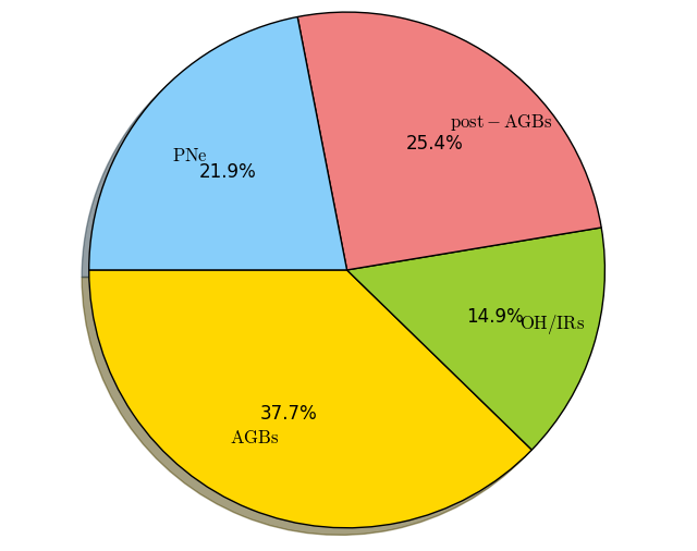
Figure 1: Pie chart illustrating the distribution of stars in the THROES sample according to their evolutionary stage.

Figure 2 shows the distribution of our targets in the IRAS two-colour diagram, where the location of various types of sources is indicated, following the original description presented by van der Veen & Habing (1988). This diagram illustrates the variety of evolutionary stages covered by the THROES sample. The AGB stars are distributed along a sequence of increasing infrared excess, which represents the evolution expected during the AGB as a result of the formation of thick and dense shells of dust and gas around these mass-losing stars, with the reddest IRAS colours corresponding to the most extreme OH/IR stars. Once the mass-loss phase ends, objects evolve towards the right in the two-colour diagram (region IV, V, and VIII in the plot), which are the areas populated by most of the sources in our sample classified as post-AGB stars and PNe, surrounded by detached cool dust shells.

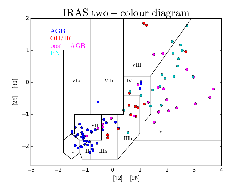
Figure 2: IRAS colour-colour diagram of the THROES sample with good quality IRAS data (Quality Flag=3) in the 12, 25, and 60 $\mu$m bands. The diagram is divided into different boxes where sources with different characteristics and evolutionary stage are contained (see van der Veen & Habing 1988, for a detailed description).

2.3.2 Galactic distribution

The galactic distribution of the THROES sample is shown in Fig. 3. Our sources are strongly concentrated at relatively low galactic latitudes, as expected from a distant population of luminous sources concentrated in the galactic disk, although a significant number of them are also observed at high galactic latitudes, corresponding to the small fraction of bright, nearby sources. Interestingly, most of the OH/IR stars are found at very low galactic latitudes, as they correspond to a population of stars that are proposed to represent the most massive precursors of PNe (García-Hernández et al., 2007).

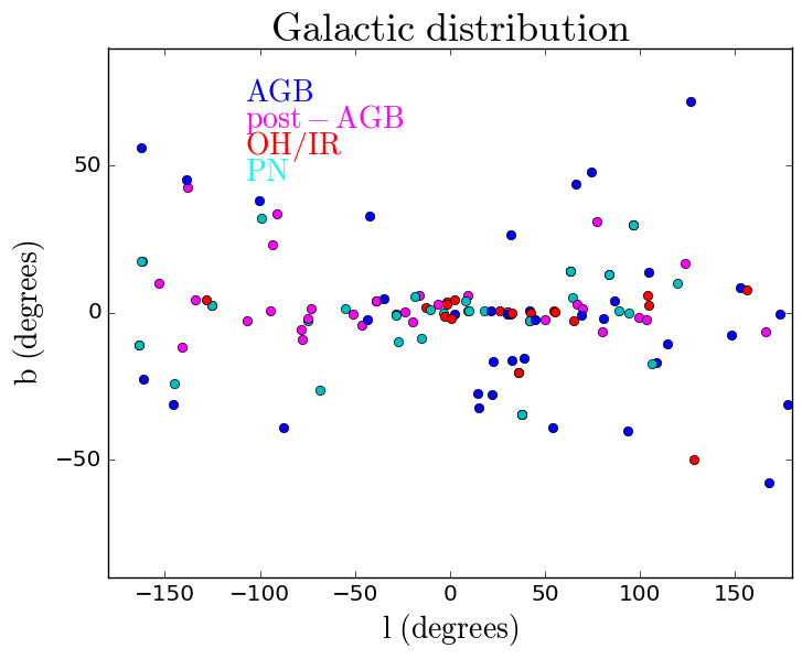
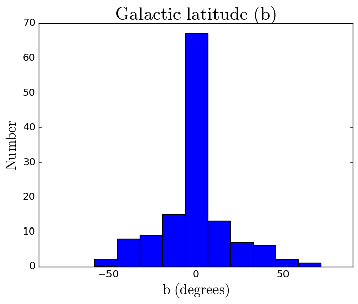
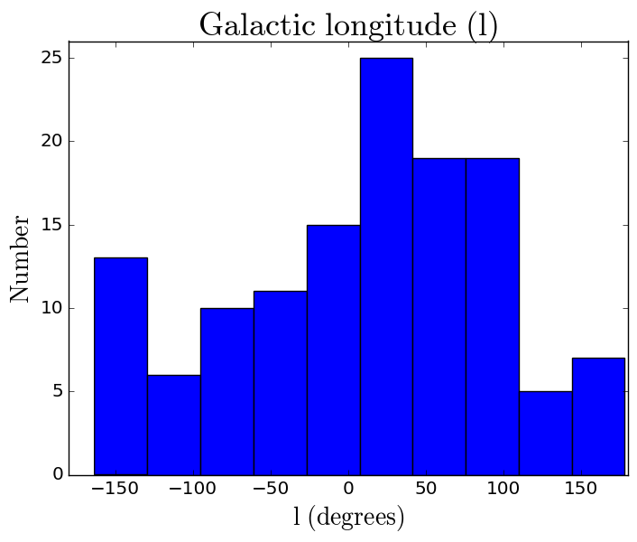
Figure 3: Galactic distribution of the THROES targets. Colour code as in Fig. 2.

2.3.3 Dominant chemistry

Asymptotic giant branch stars are generally classified as O-rich (M-type) or C-rich (C-type) based on the C/O ratio found in their outer envelope. Objects with C/O ¿ 1 are considered C-rich stars under this criterion while objects with C/O ¡ 1 are considered O-rich stars. Those sources showing C/O ratios of approximately one. are denoted as S-stars. In addition, there are also objects that present chemical indicators from both kinds of chemistries, such as the simultaneous presence of crystalline silicates, typical of O-rich chemistry, and policyclic aromatic hidrocarbons (PAHs), expected in C-rich targets, in their mid-infrared spectra. The C/O ratio in this kind of source may be different depending on the region of the source considered. Some of them are known to be objects in transition between O-rich and C-rich objects (Herwig, 2005); others display a strong bipolar morphology, and may be surrounded by disks that could explain the mixed chemistry observed. In our sample, 29$\%$ of sources are C-rich stars, 55$\%$ are O-rich stars, 3$\%$ are S-stars, 7$\%$ are sources with mixed chemistry, and 6$\%$ are sources with unknown chemistry (see Fig. 4).

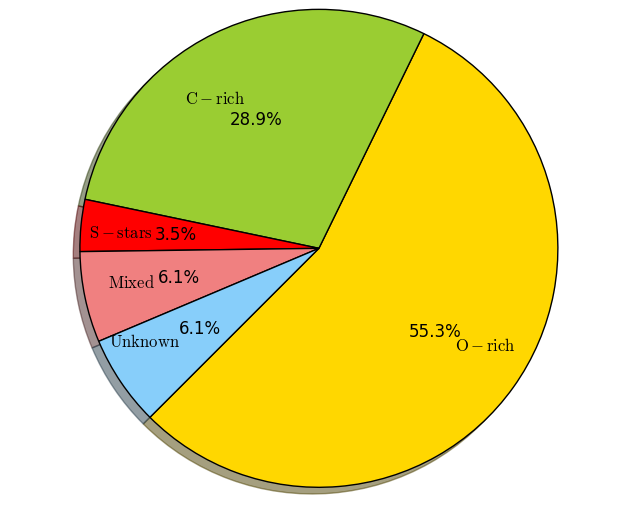
Figure 4: Pie chart illustrating the distribution of stars in the THROES sample according to their dominant chemistry.

3 Data reduction

The data available in the HSA have been generated using the latest version of the Standard Product Generator (SPG), an automated pipeline that takes the data from level 0 (raw) to level 2 (spectral cubes). At the time of starting this project, the archive was populated with products generated with HIPE 13.0.0. A complete explanation of the pipeline processing steps applied in this version of the pipeline can be found in the PACS Data Reduction Guide: Spectroscopy.

Interactive data reduction can help improve the quality of the final products by applying certain data reduction tasks not available in the automated pipeline because they require a direct interaction of the user. Therefore, we used HIPE 13.0 and version 65 of the PACS calibration files to interactively reprocess all the observations in our sample, introducing those tasks that at the moment of starting this project were not applied by the standard data reduction pipeline (version 13 at that time), with the aim of obtaining better quality products than those offered by the pipeline.

For PACS range spectroscopy observations, the interactive data reduction tasks that we have applied to improve the quality of the data can be split into two main groups:

• i) tasks applied to the spectral cubes before the level 2 data are generated, so-called, interactive re-processing.

• ii) tasks applied to the level 2 data products to extract the best 1D spectrum, so-called, post-processing.

The interactive re-processing tasks comprise:

• FlatField correction: This correction fits an n-grade polynomium to the PACS spectra to obtain a higher signal-to-noise ratio (S/N) and a better shape of the continuum.

• Telescope background correction: This correction uses the telescope background emission to flux calibrate the spectra instead of using the relative spectral response function (RSRF) applied in the SPG. This correction was later implemented in version 14 of the SPG pipeline.

To extract the final 1D spectrum from the level 2 data cubes, the following post-processing corrections were applied:

• Point source flux loss correction (PSFLC): This is needed to extract the correctly-calibrated spectrum of a point source to account for PSF losses.

• Correction for semi-extended sources (which we refer to as ”semi-extended 3x3” correction): To recover the whole flux of semi-extended sources, defined as those sources with a FWHM (Full Width Half Maximum) larger than a single spaxel (9.4”) but small enough to fill the field of view of a single pointing (about 47”x47”). This correction is also applied to try to minimize the effects of pointing jitter. The so-called semi-extended 3x3 correction is always applied after the PSFLC and the final product is a 1D spectrum labelled as ”PSFLC-3x3” corrected.

• Correction for extended sources (which we refer to as ”extended 5x5” correction): This correction was also never made available in HIPE, but we had to create it to deal with sources extended beyond the central 3x3 spaxels. It works in a similar way to the semi-extended 3x3 correction, and is also applied after PSFLC. In this case the final product is a 1D spectrum labelled as ”PSFLC-5x5” corrected.

In addition, several objects in our sample were significantly mispointed, that is, the main target was clearly not located in the central spaxel of the 5$\times$5 spaxel array of PACS. To extract the 1D spectra of these sources, we had to use a modified version of the semi-extended 3x3 correction, as we will explain in Section 3.3 in more in detail.

3.1 Spectral flatfielding

As explained in the PACS Data Reduction Guide, spectral flatfielding can be crucial for improving the continuum of the final spectra. For range scan observations, flatfielding will result in general in a better S/N, especially for the longer wavelength ranges. It will also remove the ”fringing”-like pattern that the SPG cubes often have and it will improve the appearance of sharp rises or drops in the data.

The HIPE task used for flatfield correction is specFlatFieldRange, where the user can select the order of the polynomial to fit. The default value is five but from our experience, a lower value (three or four) usually yields better results. For PacsRange observations that do not cover the whole SED of PACS, the best results are obtained using an even lower value for the order of the polynomial (normally one). We have configured the specFlatFieldRange task to exclude the regions affected by leakage (70-73 $\mu$m, 98-105 $\mu$m, and 190-220 $\mu$m); by setting the option excludeLeaks to ”True” we obtained ”clean” spectra. The exclusion of the regions affected by leaks is actually very important to obtain a correct shape of the continuum and to improve the results obtained with the specFlatFieldRange range. We note that the improvement in the S/N ratio after flatfielding is most remarkable in relatively faint sources.

3.2 Telescope background correction

This correction is needed to remove the sky and telescope background contribution. Furthermore, it uses the telescope background spectrum to flux calibrate the data, instead of using the standard calibration blocks. This process is applied using the HIPE task specDiffChop. This task computes the pairwise difference ratio: 2*(On-Off)/(On+Off), rather than the pairwise differences (On-Off) as is the case for the standard pipeline. This computation eliminates in an optimal way the detector drifts that appear in both On- and Off- positions. After this step, the flux density in the cubes is in units of ”telescope background”.

3.3 THROES post-processing

All the observations have been post-processed in different ways taking into account the nature of the object (extended or not) and the position of the source in the PACS FoV. The main goal of the post-processing was to extract, from the spectral cubes previously reduced, a 1D spectrum recovering the whole emission of the source. Depending on the post-processing tasks applied, the sources can be grouped into five main families:

• Pointed observations, good pointing, point, or semi-extended sources (PSFLC-3x3): To recover the absolute flux of a point source from PACS data, it is necessary to apply first the point source flux loss correction (PSFLC) to the spectrum extracted from the central spaxel of the final (level 2) spectral cube. This correction is needed to take into account the flux losses derived from the fraction of the PSF that falls out of the central spaxel. A theoretical PSF model is used to compute the fraction of flux seen by the central spaxel and then recover the emission that has not been detected. After this, we also need to apply the semi-extended 3x3 correction in order to recover the emission received by the spaxels around the central one in case of semi-extended sources. Both corrections are performed by the HIPE task extractCentralSpectrum, which generates three different 1D spectra:

  1) The first 1D spectrum returned by the task is simply the spectrum from the central spaxel corrected for point source flux losses.

  2) The second 1D spectrum returned contains the integrated flux of the 3x3 central spaxels (also known as ”superspaxel”) with the point source flux loss correction applied to the central one.

  3) Finally, the third 1D spectrum is the same as the first one, corresponding to the central spaxel with the point source flux loss correction applied, scaled to the flux level of the second spectrum, that of the 3x3 superspaxel. The result is the so-called semi-extended 3x3 corrected spectrum.

  Using the Semi-extended 3x3 corrected spectrum, the whole flux from sources that are slightly extended is fully recovered. An example of the differences between the 1D spectrum generated after applying this correction and the spectrum taken directly from the central spaxel of the level 2 cube before post-processing is shown in Fig. 5. The vast majority of the sources in our sample have been reprocessed in this standard way and the resulting 1D spectra are displayed in Fig. 8. An exceptional case is OH 32.8$-$0.3, for which some spaxels around the central one show negative flux values and therefore these observations have only been corrected for PSFLC (i.e. the semi-extended 3x3 correction has not been applied).
  

• Pointed observations, extended sources (PSFLC-5x5): Based on PACS photometric data, when this was available, the existing PACS spectroscopy, and the bibliography, we identified those sources in our sample that appeared more extended than just the central 3x3 spaxels. These ‘extended’ objects are: IRAS 16122$-$5122, NGC 3242, NGC 40, NGC 6445, NGC 6543, NGC 6781, NGC 6826, NGC 7009, NGC 7026, and Mz3. Due to their extension, their emission can spread sometimes over the whole PACS FoV and, therefore, for these objects, we developed a new task, the extended 5x5 correction, to scale the spectrum from the central spaxel, after applying the point source flux loss correction, to the continuum level of the 5x5 spectrum, as we did for the semi-extended 3x3 correction.
  

  As we will see in Section 5, with this new task we were able to obtain a more realistic spectrum of the extended sources in our sample, better than the spectrum generated with the semi-extended 3x3 correction, as in. this way we recovered the whole emission from the source. In Fig. 9, we show the final 1D spectra of these extended sources after applying the PSFLC and the extended 5x5 correction. The effect of this task in terms of continuum flux level recovery can be seen in Fig. 5.
  

• Pointed observations, mispointing (PSFLC-3x3): In our sample there were also seven cases of mispointed observations, namely, IRAS17347$-$3139, NGC 6302, IRC$-$10529, OH21.5+0.5, AFGL 5379, IRAS 16279$-$4757, and IRAS 13428$-$6232, for which the source is located on a spaxel different than the central one. In these cases, extractCentralSpectrum cannot be applied because, in this task, the 3x3 superspaxel is always built around the central spaxel, instead of around the one where the source is located.
  

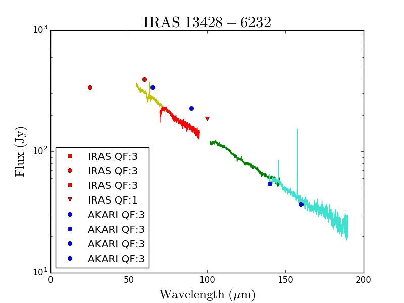
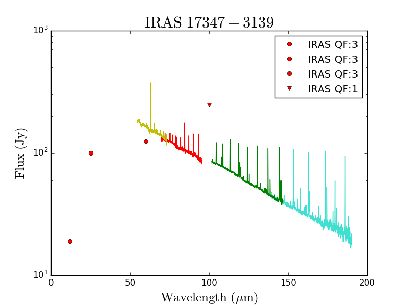
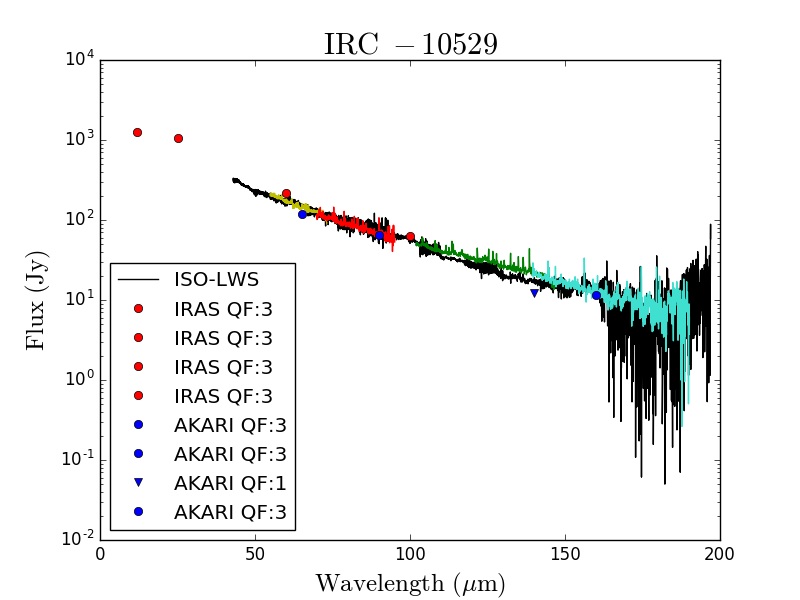
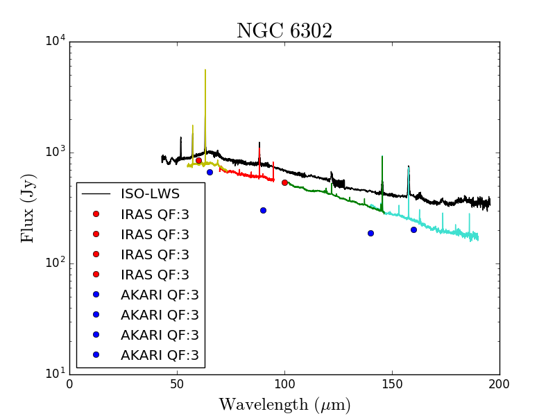
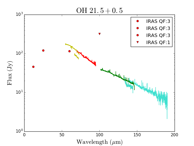
Figure 10: As in Fig. 8 but for mispointed sources after applying point sources correction and semi-extended 3x3 correction.

  To deal with these mispointed cases, we developed a script that works in a similar way to the HIPE task extractCentralSpectrum but which allows the user to select the spaxel (other than the central one) where the source is located. Our task was successfully applied to IRC$-$10529, OH 21.5+0.5, IRAS 13428-6232, NGC 6302, and IRAS 17347-3139. In Fig. 10 we show the final 1D spectra obtained after applying this correction.

  For AFGL 5379 and IRAS16279$-$4757 this correction did not work correctly as, due to the position of the sources being too far away from the central spaxel, it was impossible to generate the 3x3 superspaxel around the off-centred spaxel where the source was located.

  As was done for other observations in our sample, it is also necessary to correct these mispointed observations from PSF losses before applying the semi-extended 3x3 correction described above. To do that, HIPE provides two different tasks: extractSpaxelSpectrum and pointSourceLossCorrection. The first one takes the spectrum from the spaxel where the source is located and, after that, the second one corrects for the point source flux losses.

  Again in Fig. 5 we show the significant improvement of the final 1D spectra after applying the semi-extended 3x3 correction to mispointed observations.
  

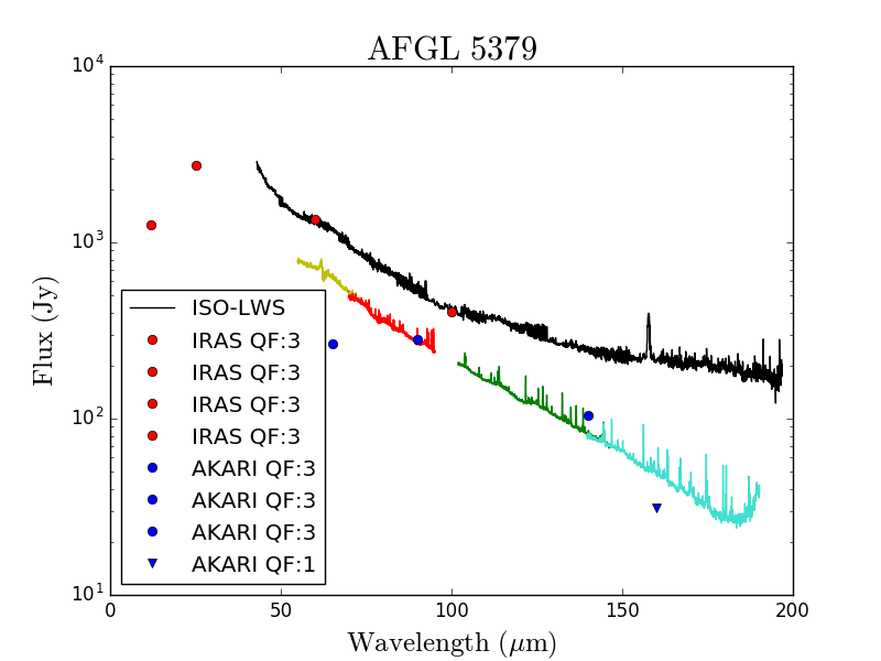
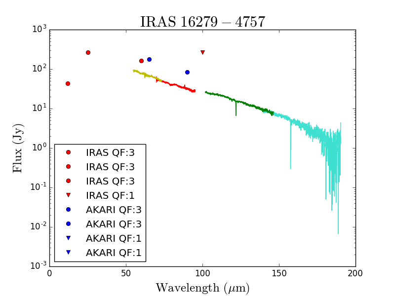
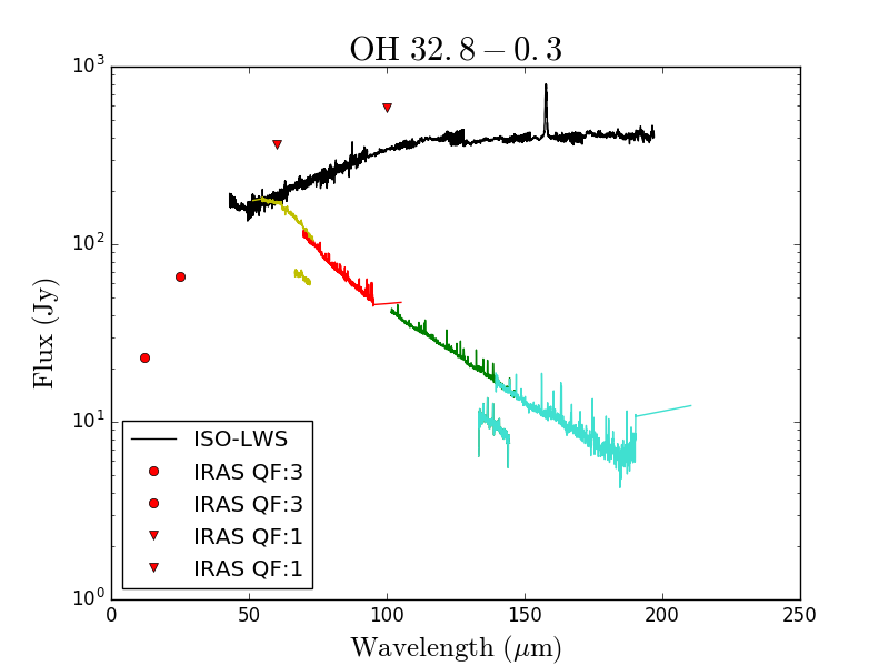
Figure 11: As in Fig. 8 but for those sources corrected only by point sources correction. AFGL 5379 and IRAS 16279-4757 are mispointed targets for which the semi-extended 3x3 correction could not be applied as they are located in one of the outermost spaxels. The well-pointed object OH 32.8-0.3 shows, for unknown reasons probably related to problems during the observations, negative fluxes in some of the 3x3 central spaxels, so the semi-extended 3x3 correction produced a wrong final 1D spectrum.

• Sources corrected only for PSFLC: Three additional sources(AFGL 5379, IRAS 16279-4757, and OH 32.8-0.3) were only corrected for PSFLC, due to different issues that prevented the application of the semi-extended 3x3 correction. These issues are related to the position of the source in the 5$\times$5 spaxels array and the presence of corrupted data in some of the spaxels needed to create the 3$\times$3 superspaxel. Their spectra are displayed in Fig. 11. For these three sources the absolute flux level of the final 1D spectrum available in the THROES catalogue should be considered only as a lower limit.
  

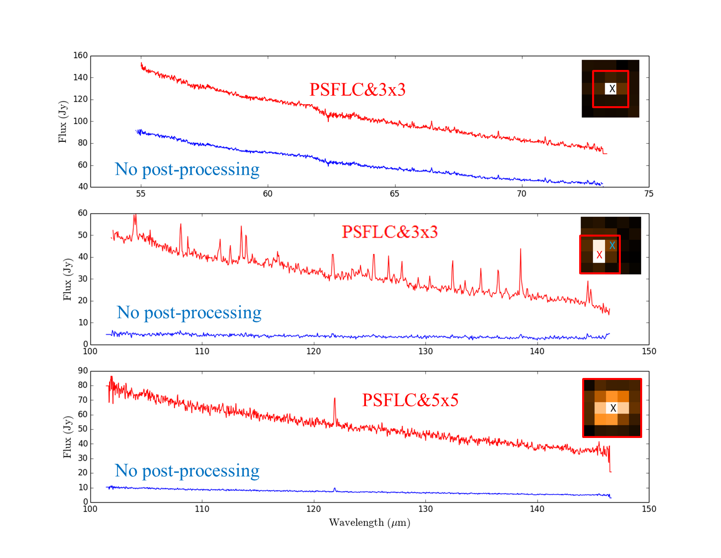
Figure 5: One-dimensional spectra extracted for three different targets in the THROES catalogue following the procedures described in Section 3 (red). The flux corrections and apertures have been chosen depending on the source extent and its location in the 5x5 spaxels FoV of PACS. For comparison, we show the corresponding spectrum obtained in each case from the central spaxel before post-processing (blue). At the top right corner of each box, we show a layer of the FinalCube with the 5x5 spaxels of the PACS spectrometer of the observation. The crosses indicate the spaxel from which the spectra were taken; a black cross means that both spectra were extracted from the central spaxel. The squares (red and blue) enclose the spaxels used for the 3x3 correction or for the 5x5 correction. Top) AFGL 3116, blue camera of PACS (ObsID: 1342212512): well pointed and semi-extended source; PSFLC-3x3 correction has been applied. Centre) Same as above but for IRC$-$10529, red camera of PACS (ObsID: 1342208931): this is a mispointed observation where the blue spectrum corresponds to that extracted from the central spaxel without post-processing, while the red one is the spectrum taken from the brightest spaxel and with the post-processing applied (PSFLC-3x3). Bottom) Same as the first two panels but for NGC 6543, red camera (ObsID: 1342238389): this is an extended source; PSFLC-5x5 correction applied.

To summarize, after our interactive data reduction process, we generated for each object the following final products:

• 1) Final spectral cubes (level 2) with the improvements that result from flatfielding and telescope background correction.

• 2) 1D spectra with the PSFLC applied, as well as the specific correction for slightly extended sources (semi-extended 3x3 correction) or extended sources (extended 5x5 correction). As a word of caution, we note that the scaling strategy followed assumes that the extension of the continuum and of the line-emitting region is roughly the same and that the spectral lines emission does not vary within the nebula, which may not be the case in some of the more extended objects. For those sources showing a more complex and extended morphology (particularly the PSFLC-5x5 corrected targets), we recommend the users to create their own 1D spectra making use of the final cubes provided in the THROES catalogue if they want to perform a more detailed analysis.

4 THROES catalogue

All the reprocessed PACS range spectroscopy observations have been compiled in a catalogue that is accessible via a web interface available at https://throes.cab.inta-csic.es/. On this web page all the reprocessed data are publicly available, including some general information about the objects and the observations made, as well as plots with the reduced PACS spectroscopy data and complementary spectroscopic and photometric observations from other observatories. A screenshot of the ‘Data Retrieval’ interface of the catalogue is shown in Fig. 6.

The tool used to create the web-based catalogue is SVOCat. This application, developed by the Spanish Virtual Observatory (SVO) is designed to make the publication of an astronomical catalogue easier, both as a web page and as a Virtual Observatory Cone Search service. Our archive system has been designed following the IVOA (International Virtual Observatory Alliance) standards and requirements. In particular, it implements the Cone Search protocol, a standard defined by the IVOA for retrieving records from a catalogue of astronomical sources. Queries made through the Cone Search service are based on the description of a sky position and an angular distance, defining a cone on the sky. The response returns a list of astronomical sources from the catalogue whose positions in the sky lie within the pre-defined cone, formatted as a VOTable (Virtual Observatory Table). The system as a whole is included in the IVOA Registry and can therefore be discovered by any VO-tool.

To structure our catalogue in a homogeneous and logical way, all the observations with the same pointing have been grouped into a unique entry in the archive. Therefore, there is a single line per region in the sky observed. As we can see in Fig. 6, there are 13 columns for each entry, each providing information about the object or the observation as well as links to plots and to the reprocessed data. Each of the columns contains the following information:

• Columns 1 to 4: The equatorial coordinates (right ascension and declination) of the observation in different units: decimal degrees in columns 1 and 2, and hh:mm:ss and dd:mm:ss in columns 3 and 4.

• Column 5: Name of the object in the THROES catalogue.

• Column 6: The astronomical observation template (AOT). This could be PacsRange or PacsLine. For some objects there are spectra taken in both modes. These cases appear in the catalogue as PacsLine/PacsRange. Only the PacsRange spectra have been reprocessed in the current version of the THROES catalogue.

• Column 7: The number of observations taken in that position of the sky. By clicking on the number shown in this column, a new table is deployed with detailed information for each observation, such as: target name, equatorial coordinates (RA and Dec), proposal name, AOT, observation ID, observing date and time, and original AOR (Astronomical Observation Request) label.

• Column 8: Mass classification (based on the bibliography and SIMBAD). The options are: evolved low-intermediate mass star, evolved massive star, or unknown.

• Column 9: Object classification including the evolutionary stage and its dominant chemistry (based on the bibliography and SIMBAD), the options are: O-rich AGBs, C-rich AGBs, S stars, OH/IR stars, O-rich post-AGBs, C-rich post-AGBs, mixed chemistry post-AGBs, O-rich PNe, C-rich PNe, mixed chemistry PNe, or Unknown.

• Column 10: This column indicates if the observations have been reprocessed under the THROES project or not. This is because THROES may be expanded in the future to other observing modes of PACS and/or massive evolved stars.

• Column 11: By double clicking on ‘SED’, a pop-up window is displayed showing the 1D PACS spectra generated after the interactive data reduction and subsequent post-processing, together with complementary photometric (IRAS and AKARI) and spectroscopic (Infrared Space Observatory-Long-Wave Spectrometer (ISO-LWS)) data, when available.

• Column 12: By double clicking on ‘CSV’ (Comma-Separated Values), a compressed folder with the name of the target is downloaded containing a gzipped tar file with the 1D PACS spectra, in CSV format.

• Column 13: Similarly, by double clicking on ‘FITS’ (Flexible Image Transport System), a compressed gzipped tar file is downloaded containing the THROES reprocessed final spectral cubes (level2) in FITS format and the 1D PACS spectra, also in FITS format, derived from these final spectral cubes after post-processing.
  

More information about how to query the catalogue through the different search fields is available in the documentation available on the THROES catalogue web page.

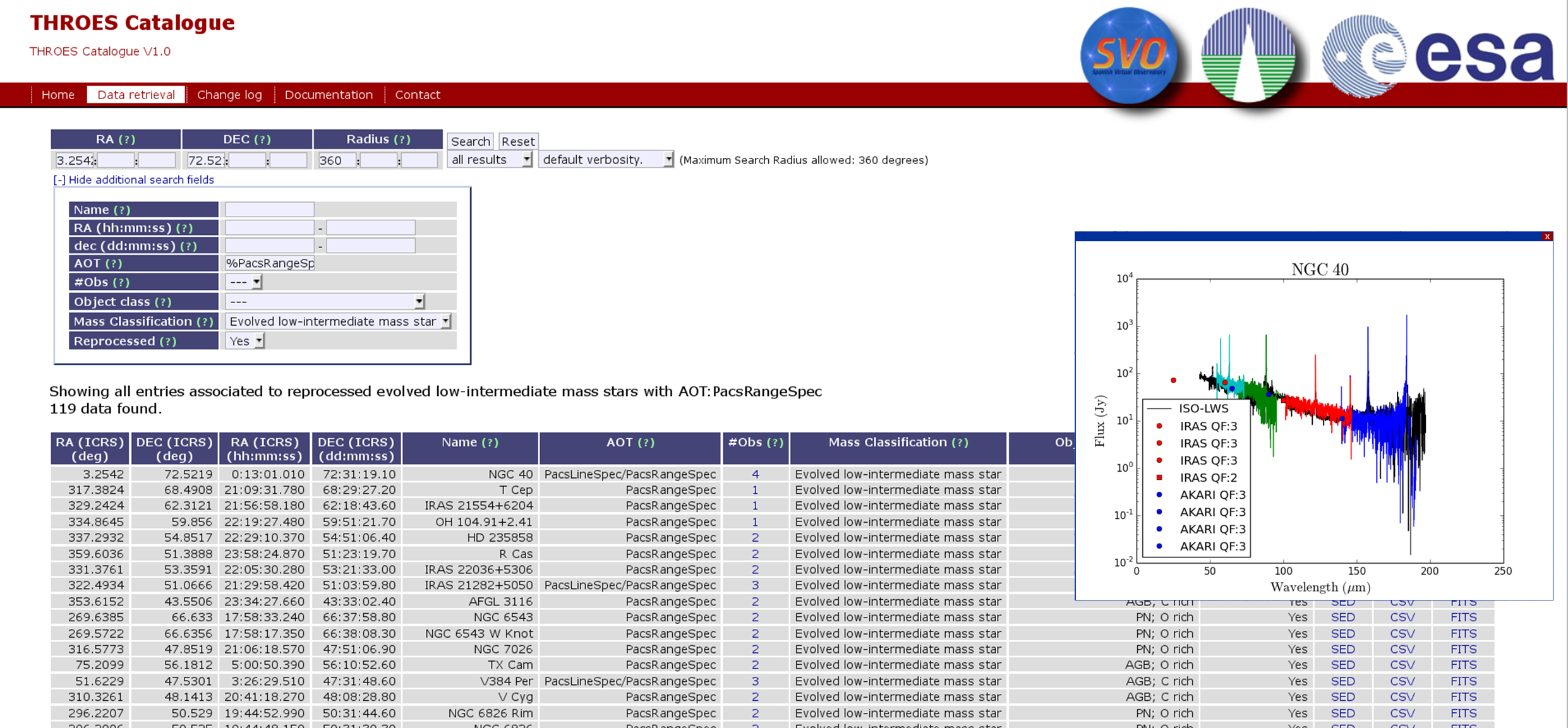
Figure 6: Screenshot of the THROES catalogue web interface. All the columns and search fields described in Section 4 are shown as well as an example of a complete SED with IRAS and AKARI data overplotted.

5 Characterization of the THROES sample

All the individual THROES spectra are shown from Figs. 8 to 11. To illustrate the quality of the resulting spectra, every plot contains not only the final PACS 1D spectra, but also the photometric (IRAS and AKARI) and spectroscopic ISO-LWS data, whenever these are available. In Table. LABEL:THROESSampleInfo we display information associated to the PACS, ISO (Infrared Space Observatory), IRAS, and AKARI data used for the generation of the SEDs.

5.1 Comparison with IRAS and AKARI photometry

All the objects in the THROES catalogue have complementary IRAS photometric information while, for AKARI data, the percentage of common objects decrease to 89$\%$. The Infrared Astronomical Satellite (IRAS) (http://irsa.ipac.caltech.edu/IRASdocs/iras.html) point source catalogue presents photometric data in four bands centred at 12, 25, 60, and 100 $\mu$m. The beam size of IRAS observations, which is much larger than that of PACS, varies from 2’ at shorter wavelengths to 5’ at longer ones (Jeong et al., 2007). AKARI (http://www.ir.isas.jaxa.jp/AKARI/index.html) covers longer wavelengths, 65, 90, 140, and 160 $\mu$m, and the beam size varies from 0.5’ to 0.9’ (Jeong et al., 2007). The different beam sizes of the instruments is a key point that has to be kept in mind when comparing PACS spectroscopy to IRAS and AKARI photometric data.

In order to check the quality of the final processed PACS spectroscopy data and to obtain information about the effect of the post-processing tasks applied to generate the final 1D spectra, a comparison between the synthetic photometry derived from the PACS spectroscopic data and the IRAS and AKARI photometric data at 100 and 160 $\mu$m, respectively, has been done.

Synthetic photometry is generated by convolving the transmission curve of the photometric filters, IRAS₁₀₀ and AKARI₁₆₀, with the 1D PACS spectra. The transmission curve of IRAS₁₀₀ has been obtained from:
http://irsa.ipac.caltech.edu/IRASdocs/exp.sup/ch2/ tabC5.html and the transmission curve of AKARI₁₆₀ has been estimated from the relative response function available in:
http://svo2.cab.inta-csic.es/theory/fps3/ ?id=AKARI/FIS.N160.

As the synthetic photometry requires a convolution between the 1D PACS spectrum and the curve of the photometric filters, it is necessary that the PACS spectrum spectral coverage extends, at least, along the whole wavelength subrange covered by the photometric filters. For this reason, the synthetic photometry can be estimated for the subsample of 71 THROES targets with full spectral coverage of the PACS wavelength range.

As mentioned in Section 3, due to the instrument configuration and the exclusion of some sub-regions affected by leakage, all the 1D PACS spectra show a small gap (less than 10 $\mu$m) around 100 $\mu$m, even for those sources that present a complete spectral coverage. As the photometric curve of IRAS 100 $\mu$m is centred on this region, it is important to find a solution. To cope with that in the synthetic photometry estimation, a linear interpolation was done to approximate the continuum flux level in this region. This assumption is good enough as intense emission lines are not expected in this region.

On the AKARI 160 $\mu$m side, due to the exclusion of the wavelength regions affected by leakage, there are no PACS data to cover the wavelength range from 190 to 220 $\mu$m. To solve that, a power law ($\lambda^{\alpha}$) was fitted to the red bands of the PACS SED and, after that, we extrapolated the flux values to the 190-220 $\mu$m region. At these wavelengths, we are mainly tracing the Rayleigh-Jeans emission, so this extrapolation is reasonable.

To show the effect of the post-processing tasks applied in the THROES reduction process, the synthetic photometry has been estimated for 1D PACS spectra before and after applying the post-processing tasks. In Fig. 7 the comparison between IRAS₁₀₀ and AKARI₁₆₀ photometric data and their synthetic counterparts using PACS data with and without post-processing is shown. We can see clearly that a disagreement between the photometric and the synthetic photometric data, before post-processing, is obtained. This disagreement is significantly reduced after post-processing tasks are applied, so it confirms that the tasks introduced in the reduction process of THROES are needed for reliable absolute flux calibration. The few points that fall out of a one-to-one observational-to-synthetic photometry relation are points that have bad IRAS and/or AKARI photometric data, (Quality Flag$\neq$3, red triangles) or are associated to extended objects (blue crosses).

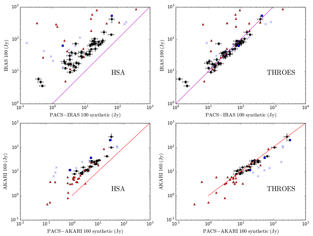
Figure 7: Comparison of IRAS (100 $\mu$m) and AKARI (160 $\mu$m) photometry with synthetic PACS photometry at these wavelengths before (left) and after (right) the interactive reprocessing of the data carried out in this work and that is available through the THROES catalogue. The objects plotted here are those which present a complete coverage of the PACS spectral range. We have established a code to distinguish the extended objects (blue crosses), the mispointed ones (red squares), the objects with bad IRAS₁₀₀ or AKARI₁₆₀ data (Quality Flag$\neq$3, red triangles), and objects with good IRAS₁₀₀ or AKARI₁₆₀ data (Quality Flag=3, black circles with error bars). The solid line represents a perfect match (1:1 ratio) of the synthetic (PACS) and observational photometric (IRAS and AKARI) points.

5.2 ISO-LWS spectroscopy

It is interesting to compare our PACS spectroscopic data to ISO-LWS spectra, since this instrument covers a wavelength range from 43 to 197 $\mu$m that almost fully overlaps with PACS. However, it is important to keep in mind that ISO-LWS presents a worse spectral resolution, R=200 (medium resolution) and R=1000 (high resolution), and a larger beam size (80”$\times$100”).

Whenever available, ISO spectra are shown in Figs 8 to 11 together with our 1D PACS spectra and IRAS/AKARI photometry points. After a visual inspection of those objects which present both PACS and ISO data, objects can be grouped into five main families:

1. Good agreement between PACS and ISO: For most of the sources, a good agreement between PACS and ISO-LWS spectroscopic data is found. For example, HD 161796, CIT 6, AFGL 618, or CPD -568032 (see Fig. 8).

2. Mispointed PACS observations without 3x3 correction: Due to its location close to the edge of the PACS 5$\times$5 array, it was not possible to apply the semi-extended 3x3 correction to one source, AFGL 5379. This could explain why the continuum flux level of the ISO-LWS is higher than that of the PACS spectrum (see Fig. 11).

3. Background contamination of the ISO spectra: One of the most remarkable facts found with this comparison is that, for some sources, the ISO-LWS spectra show a continuum level higher than the one of PACS. This effect seems to be more evident at longer wavelengths (¿ 100 $\mu$m). Besides, for all these spectra we find an emission line at 158 $\mu$m associated to [C ii] due to interstellar emission, so the origin of this extra contribution could be the contamination of the interstellar medium. There are 11 sources that have been classified in this group: AFGL6815, IRAS 16342-3814, IRAS 16594-4656, IRAS 22036+5306, IRAS 21282+5050, MWC 922, NGC 6537, NML Cyg, OH 26.5+0.6, OH 32.8-0.3, and V Cyg. The reason why ISO-LWS spectra show this contamination is the larger FoV of ISO-LWS with respect to the PACS FoV (see Figs. 8 to 11).

4. Very extended sources: Extended sources in THROES sample have been corrected using the extended 5x5 correction to recover the whole flux taken by PACS spectroscopy. However, there are some objects, such as NGC 6781, that are even larger than the PACS FoV and, therefore, PACS spectroscopic data do not measure all the flux emission from the source in contrast to ISO-LWS, which has a larger beam. For that reason, for these very extended sources, the continuum flux level of the ISO-LWS spectra is higher than that of PACS (see Fig. 9).

5. Bad ISO data: Finally, for some sources like IRAS 07027-7934 or HD 56126, ISO-LWS data present evident artefacts that make the ISO spectroscopic data unreliable (see Fig. 8).

6 Summary

We made an inventory of all the observations of all evolved stars taken in standard mode by Herschel with PACS spectroscopy. From all of them, we selected pointed, Chop/Nod, and PacsRange observations of evolved low-to-intermediate mass stars and we interactively processed the resulting 220 individuals Herschel/PACS Obs IDs, corresponding to 114 different targets.

Along the reduction process we introduced new tasks to improve the final PACS spectroscopy products. These tasks can be divided into two main groups:

• 1) Tasks applied to the spectral cubes before the level 2 data are generated: flatfield correction and telescope background correction.

• 2) Tasks applied to the level 2 data products to extract the best 1D spectrum (post-processing). These tasks try to recover the whole flux of the sources within the PACS 5$\times$5 spaxels array, taking into account the extension of the emission and the position of the object in the PACS FoV. They are: point source flux loss correction (PSFLC), semi-extended 3x3 correction, and extended 5x5 correction.

After the interactive data reduction, we generated synthetic photometry to compare our final THROES 1D spectra to photometric, IRAS₁₀₀ , and AKARI₁₆₀ photometric data. THROES 1D spectra were compared also with spectroscopic (ISO-LWS) data. From these comparisons we can conclude that our re-processing generates improved quality products compared with those routinely generated by the SPG in an automated mode, available in the HSA, and are in good agreement with IRAS and AKARI photometric data. Furthermore, the comparison of PACS with ISO-LWS spectra has highlighted the presence of interstellar contamination in some ISO-LWS data.

To ease the access to the final spectral cubes (level 2) and to the post-processed 1D spectra, we have created a web-based interface using SVOCat. Through https://throes.cab.inta-csic.es/, all the products generated as a result of the THROES interactive data reduction process are available. The THROES catalogue is expected to be updated in the near future by extending the analysis to new spectroscopic data from other instruments such as SPIRE. Furthermore, there is the potential to extend the analysis to evolved massive stars.

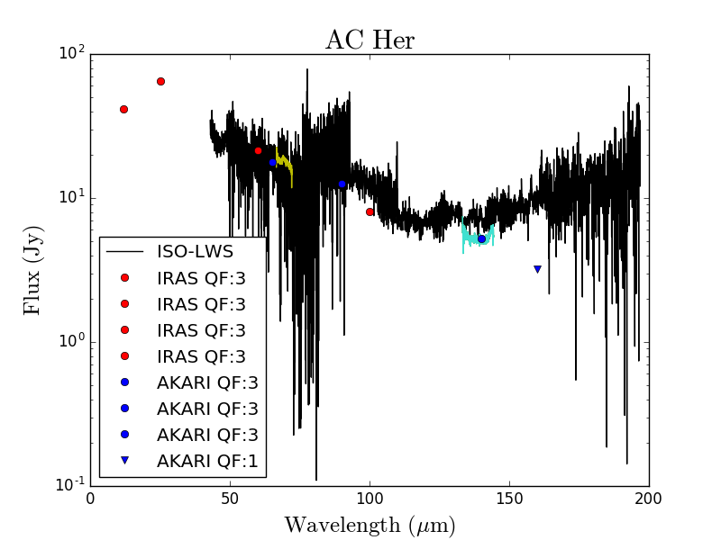
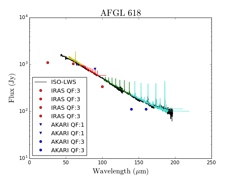
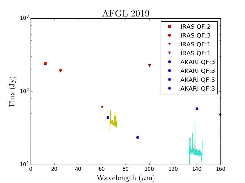
Figure 8: PACS spectroscopy SED of well-pointed, non-extended sources, after applying PSFLC and semi-extended 3x3 correction (PSFLC-3x3). PACS data is colour-coded according to the spectral region covered by each subrange, as follows: $\sim$50-70 $\mu$m (yellow), $\sim$70-100 $\mu$m (red), $\sim$100-145 $\mu$m (green), and $\sim$145-200 $\mu$m (turquoise). IRAS (red points) and AKARI (blue points) photometric data and ISO (black) spectroscopic data are also displayed when available. We do not show those observations pointed to a specific region in the case of very extended sources such as rims or knots.

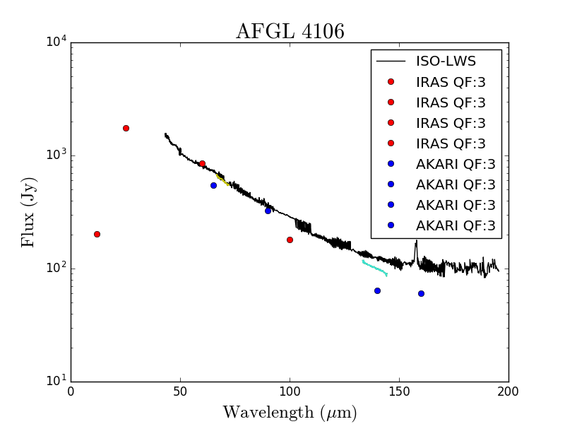
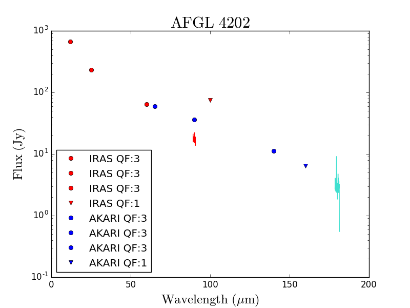
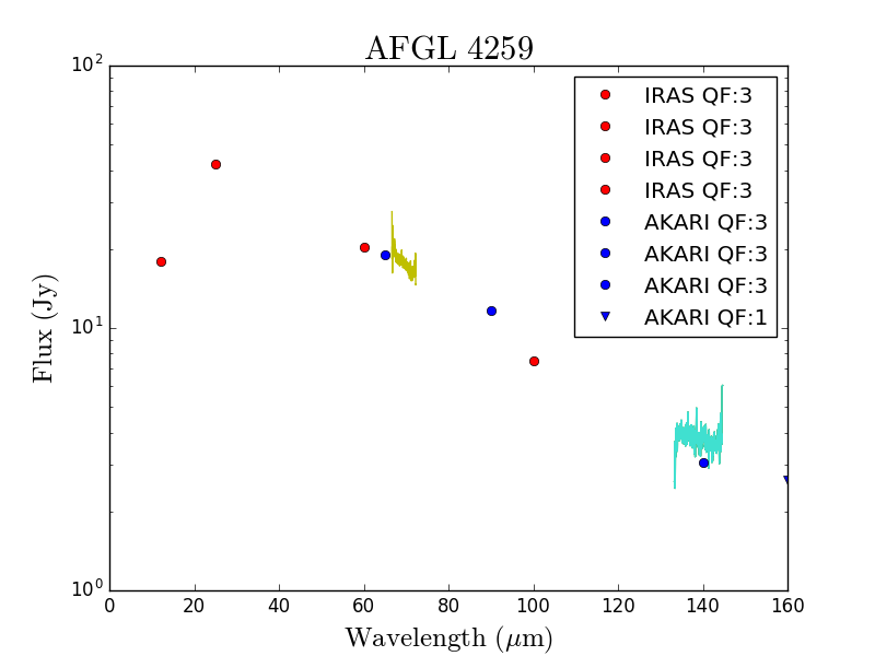
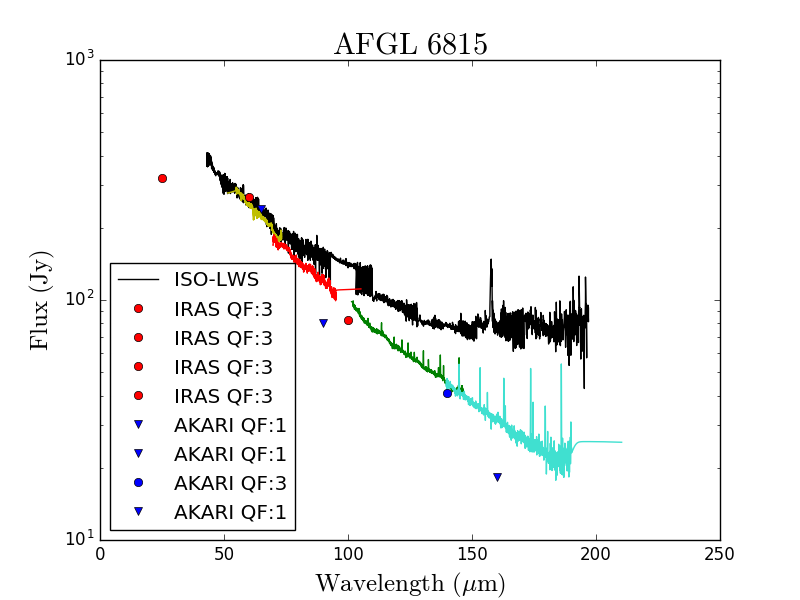
Figure 8: Continued.

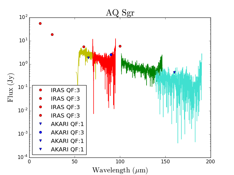
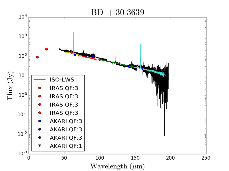
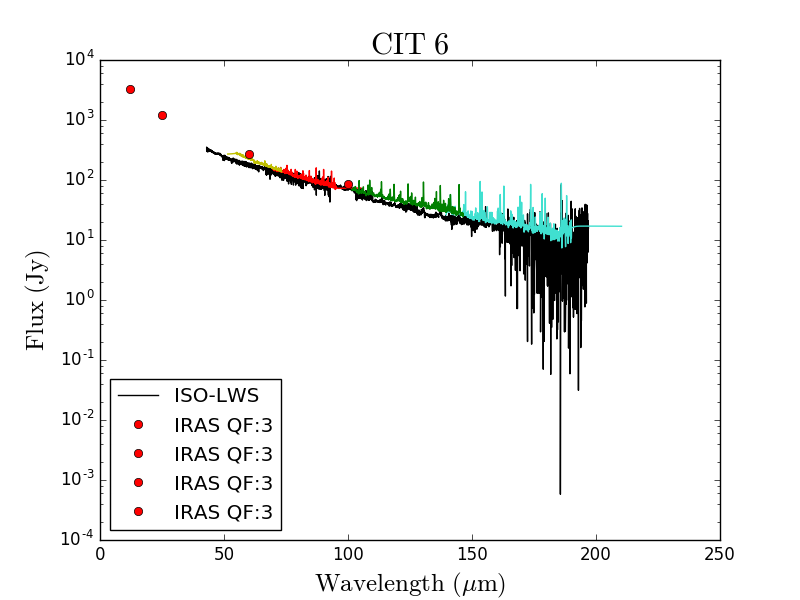
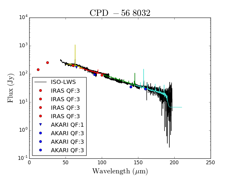
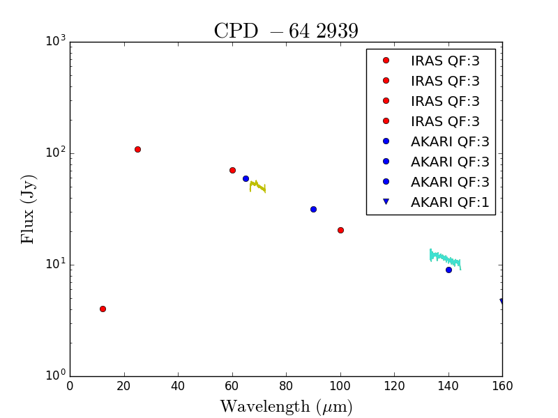
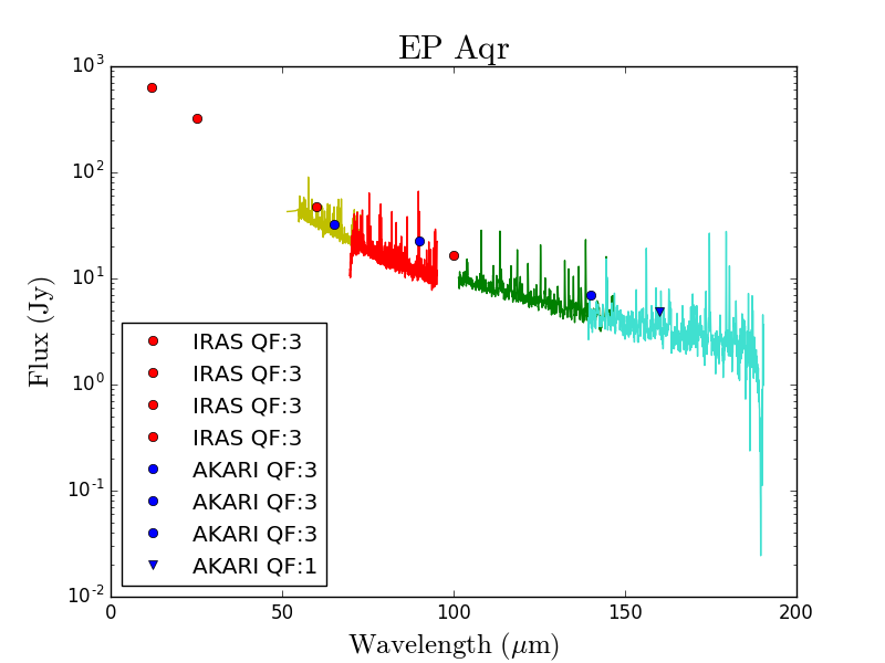
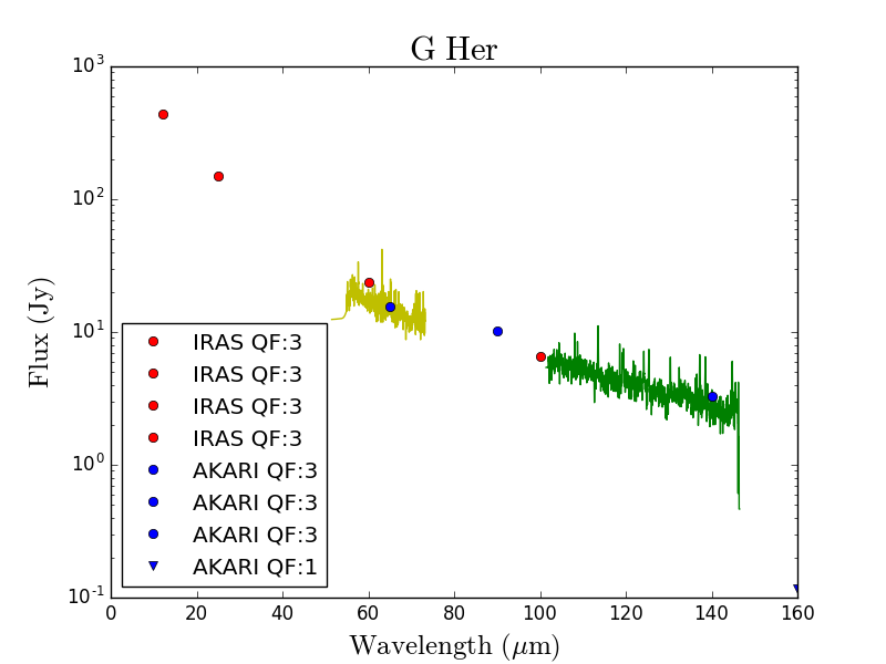
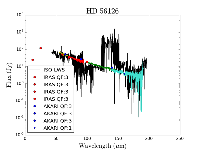
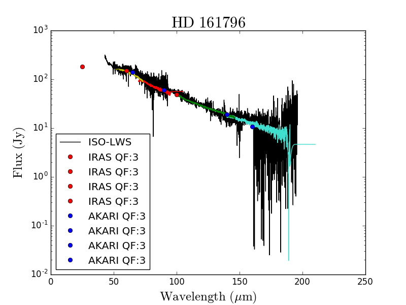
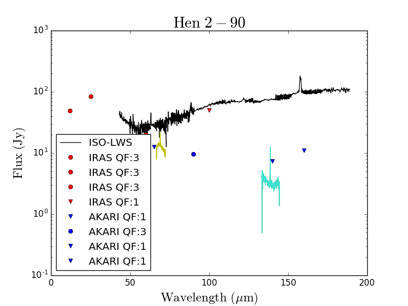
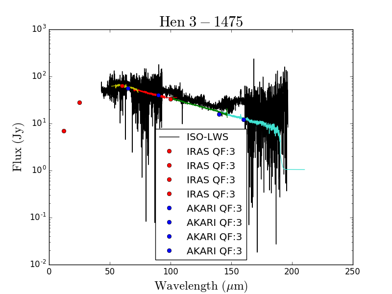
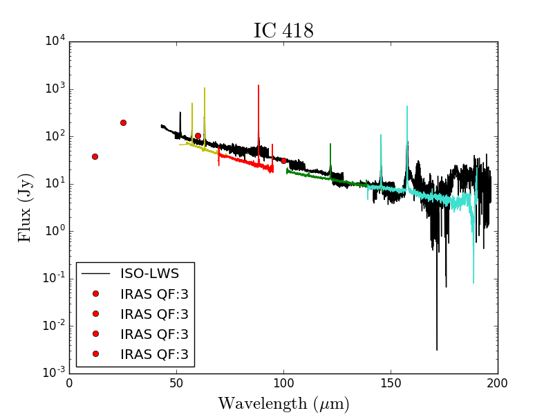
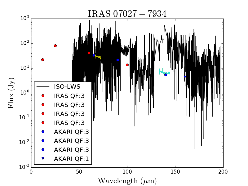
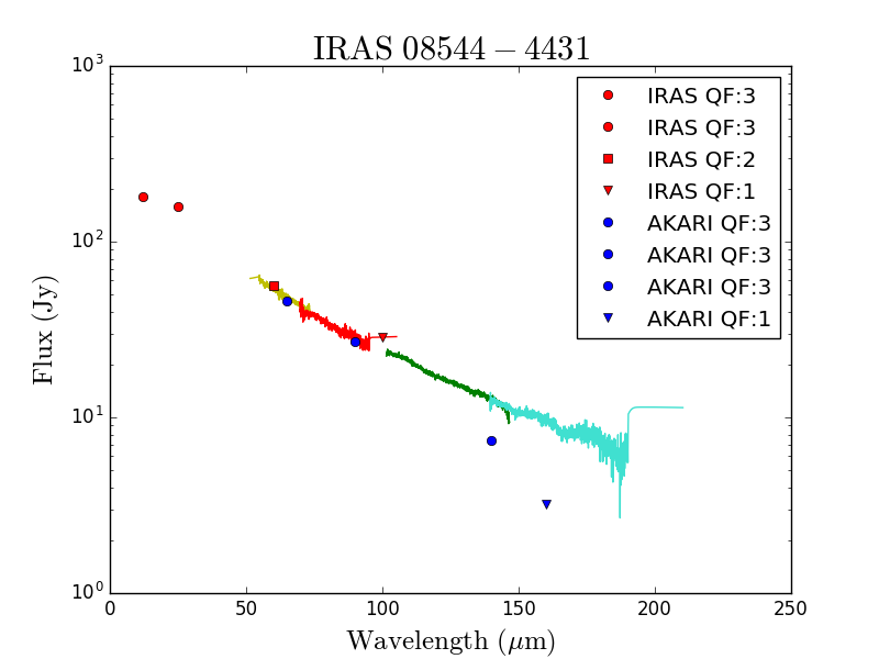
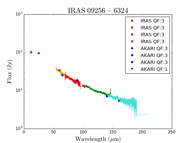
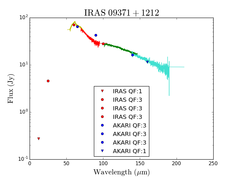
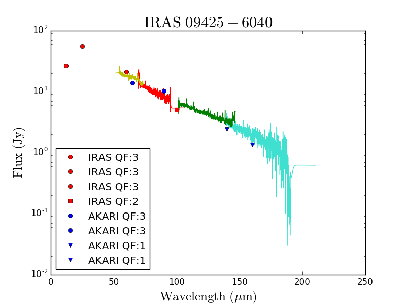
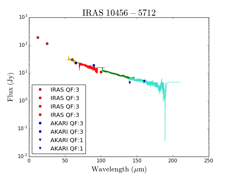
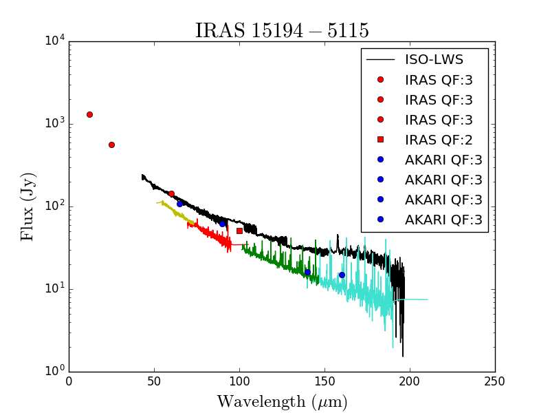
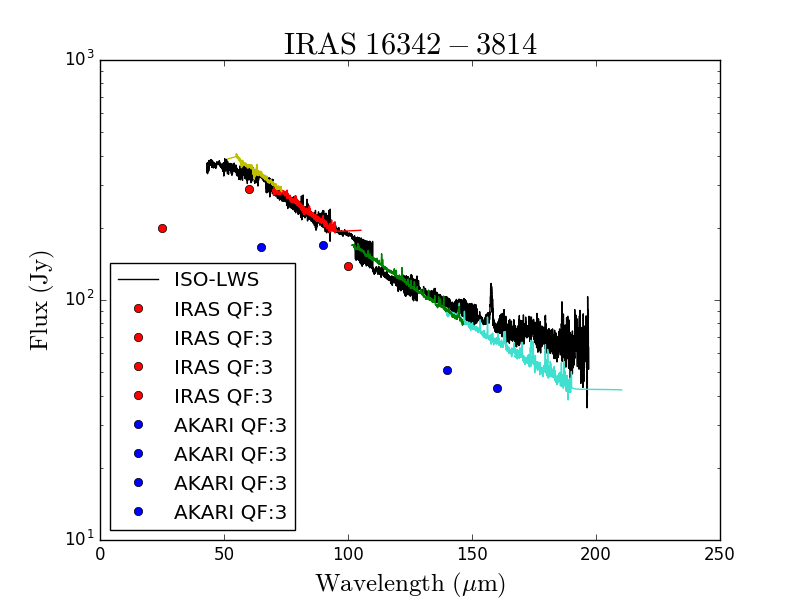
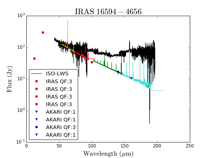
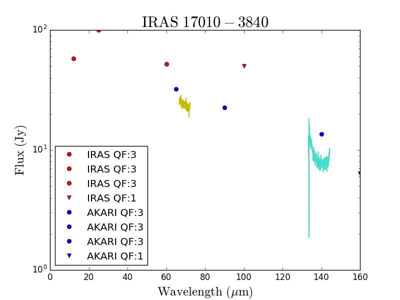
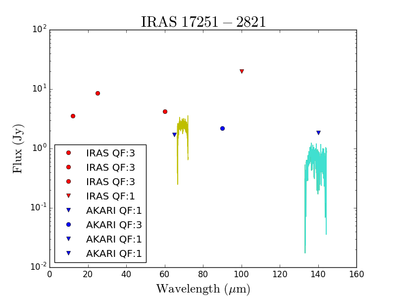
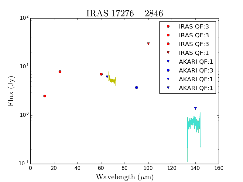
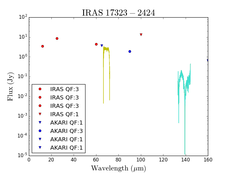
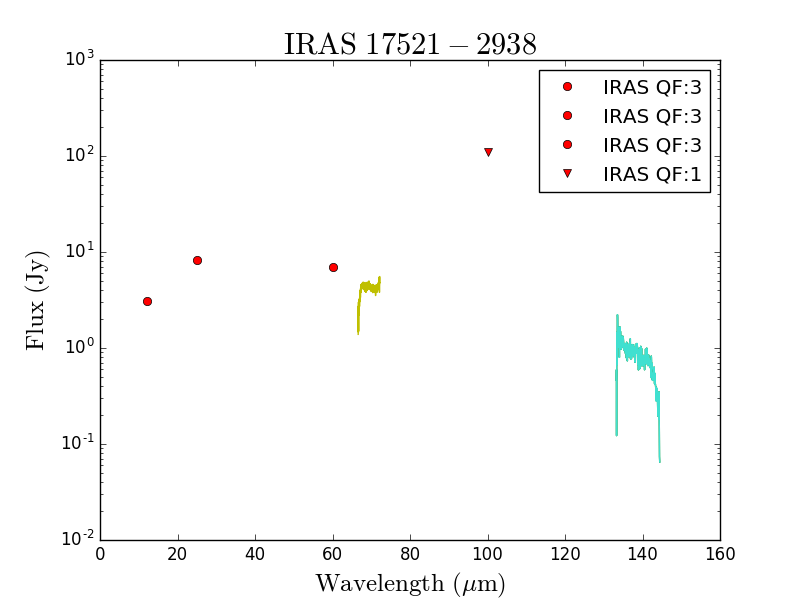
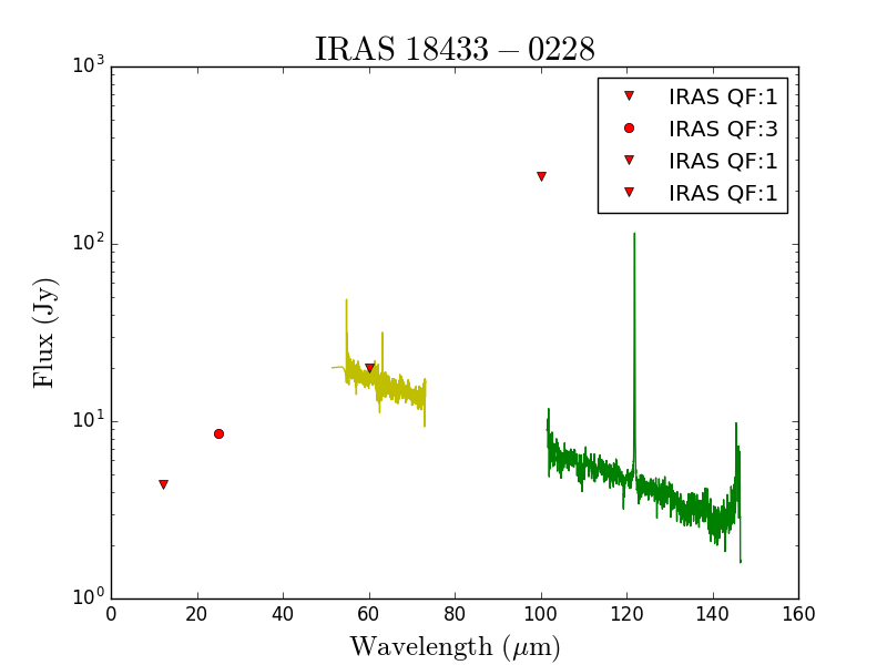
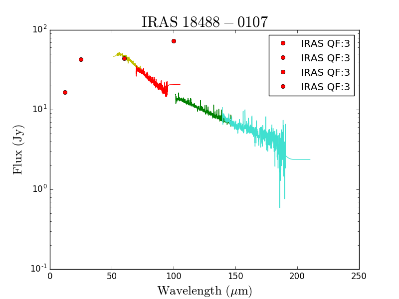
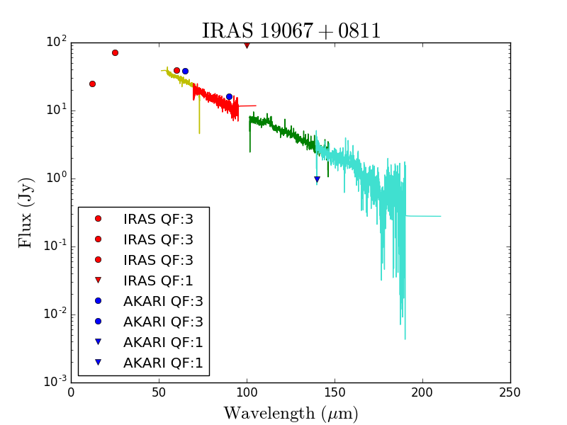
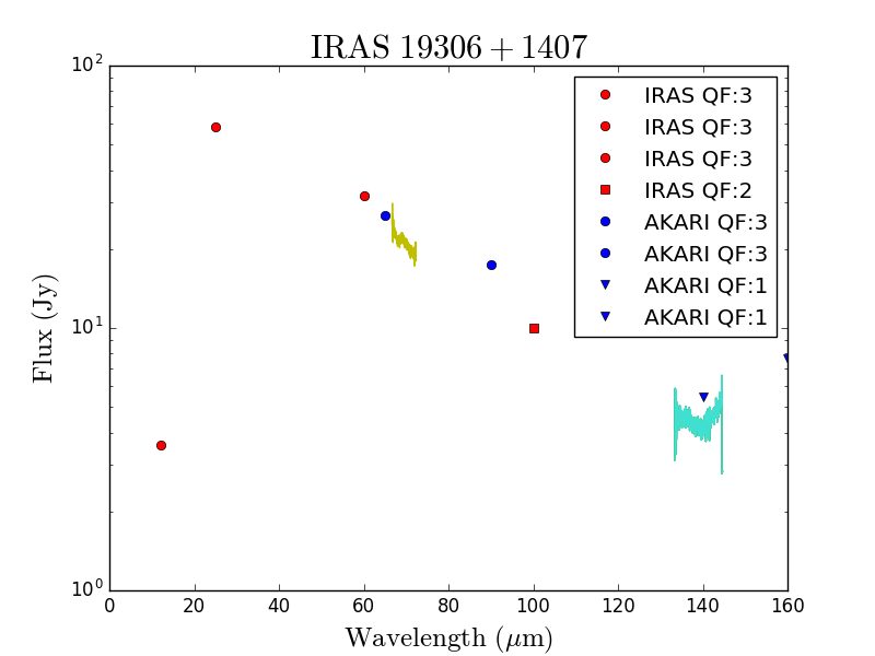
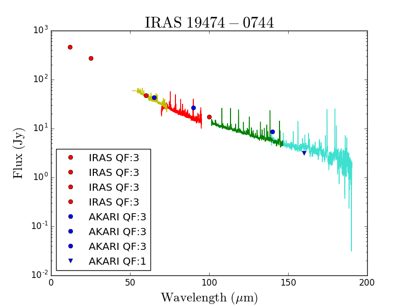
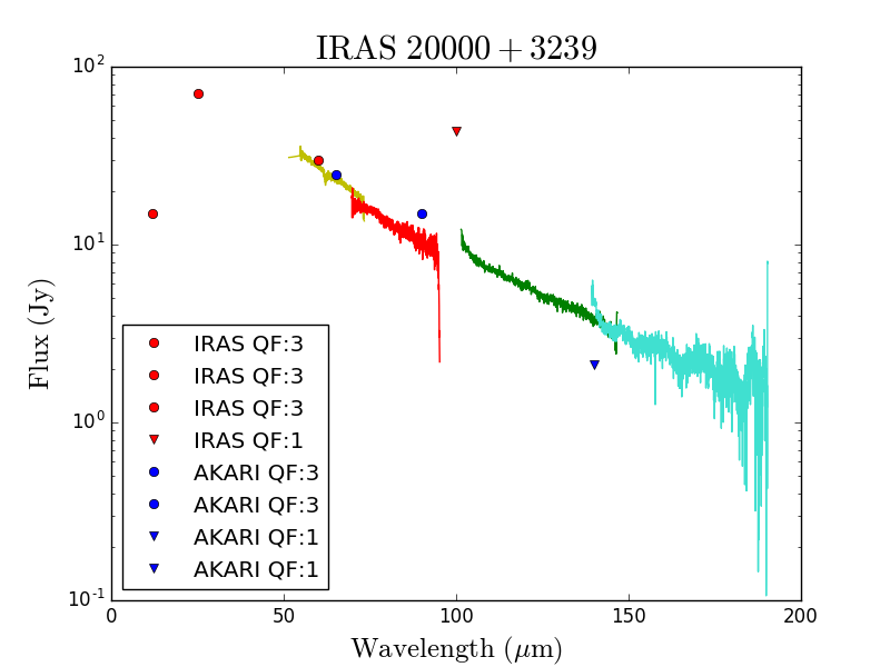
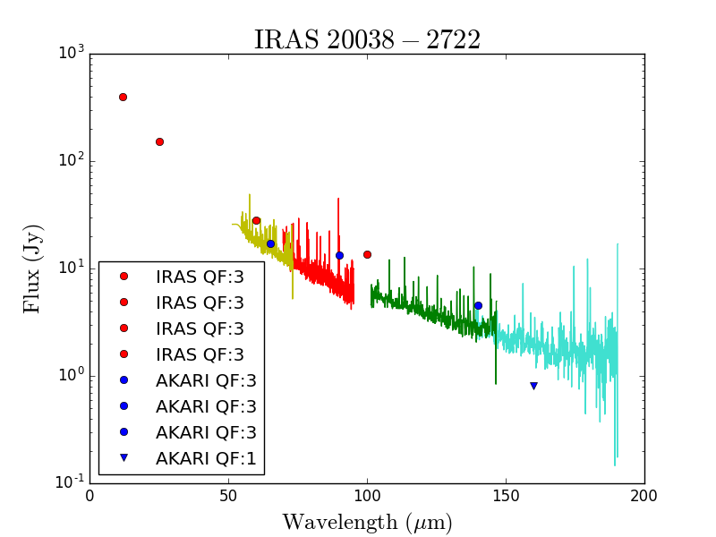
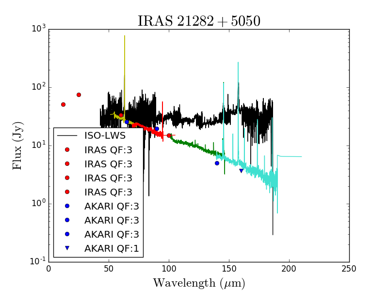
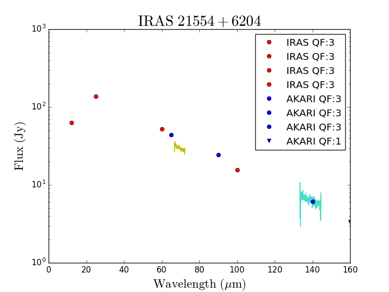
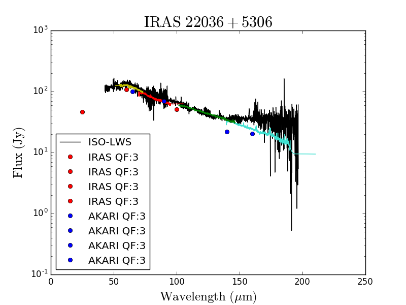
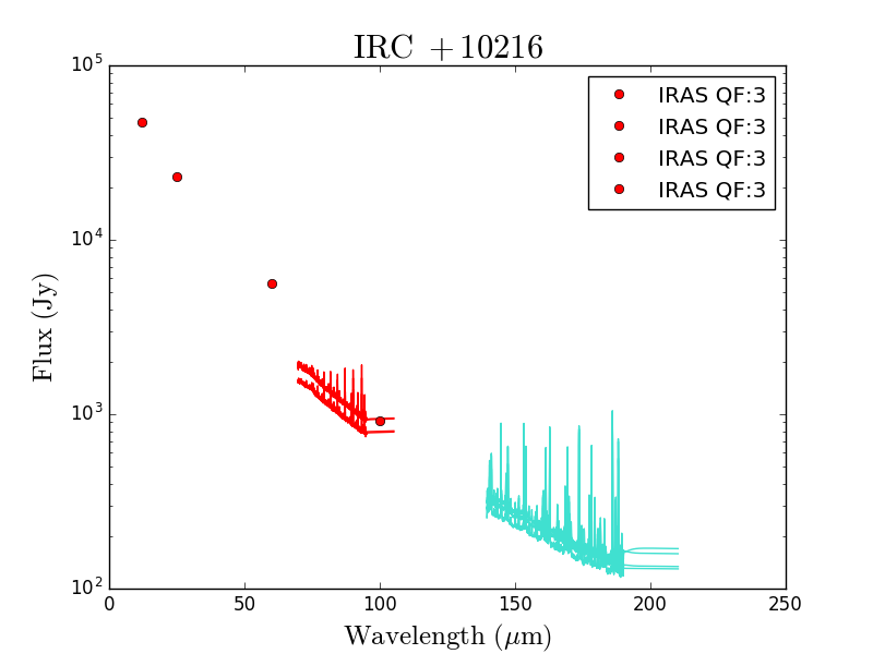
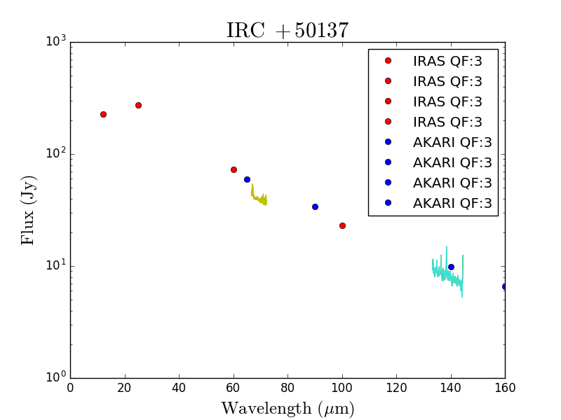
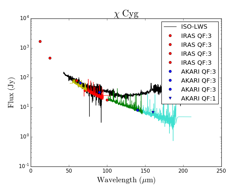
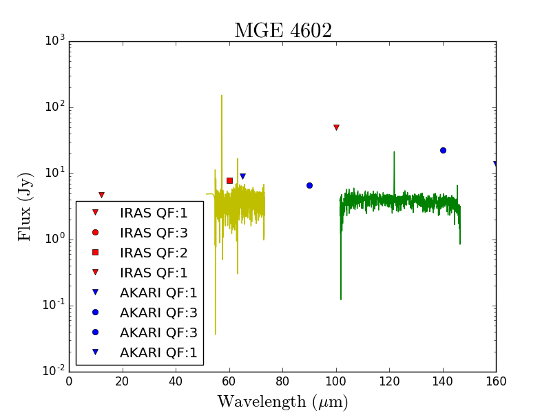
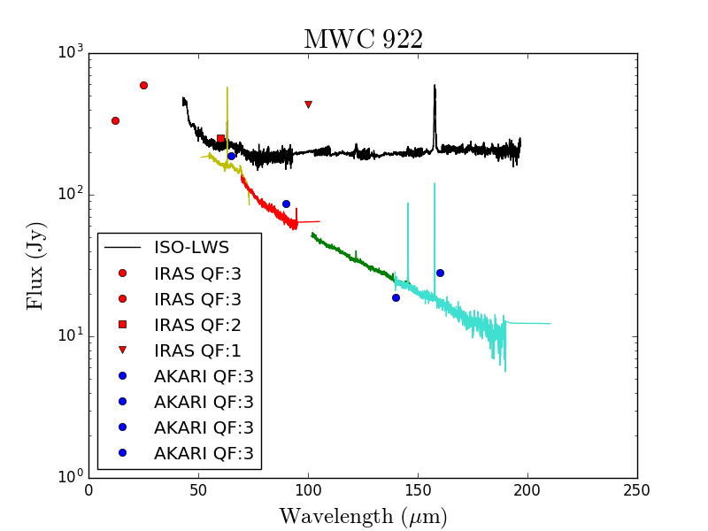
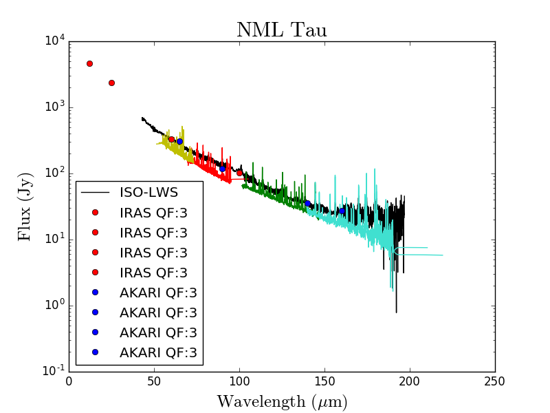
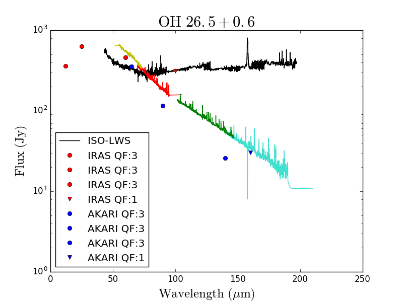
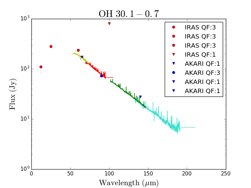
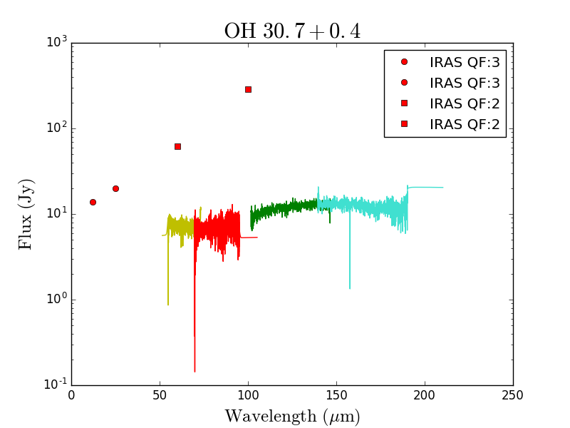
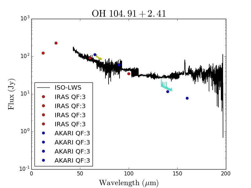
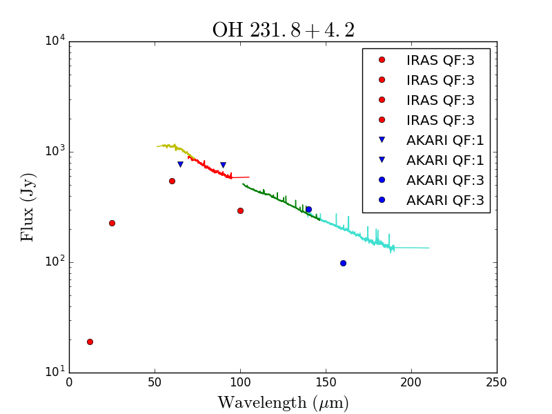
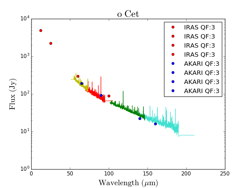
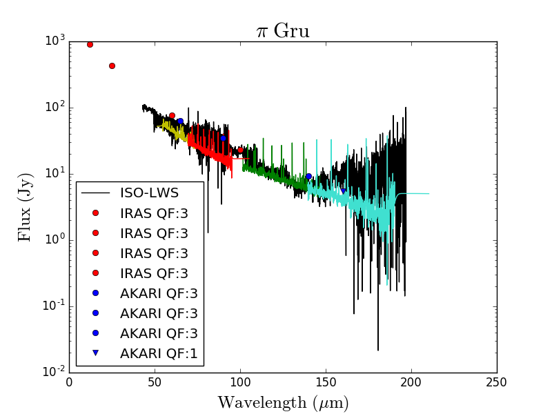
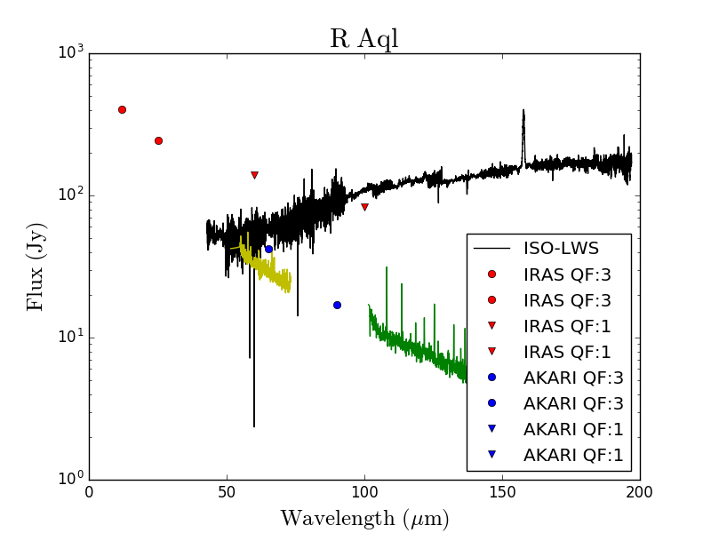
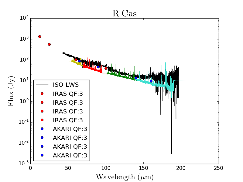
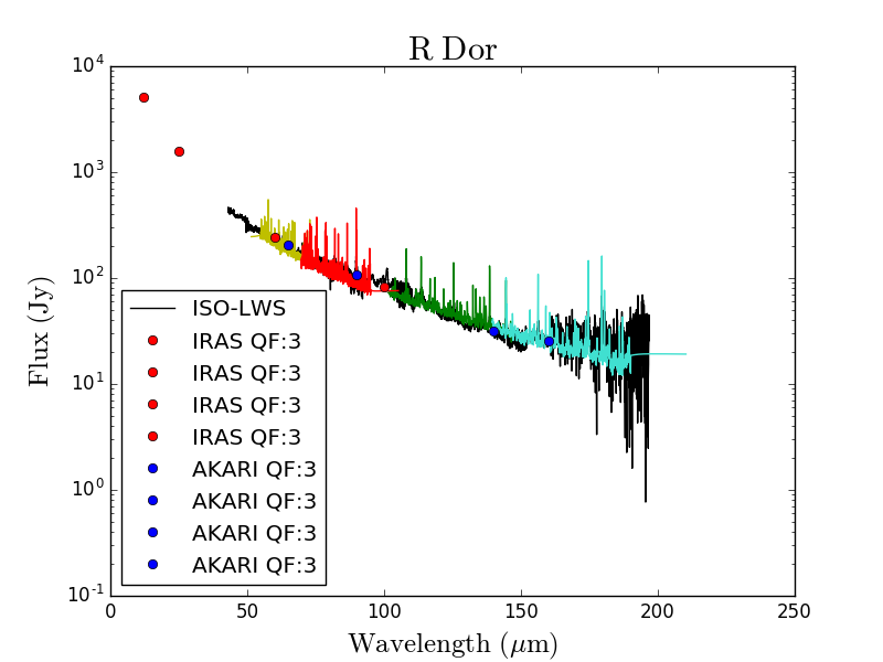
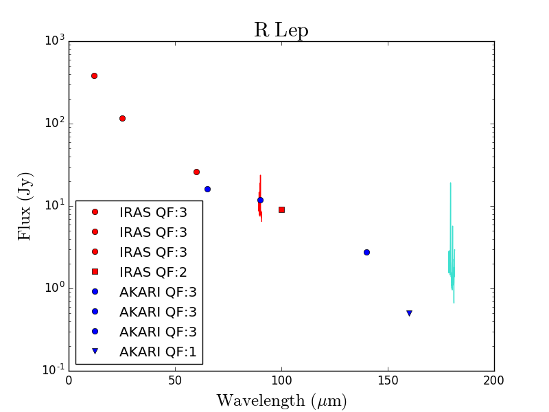
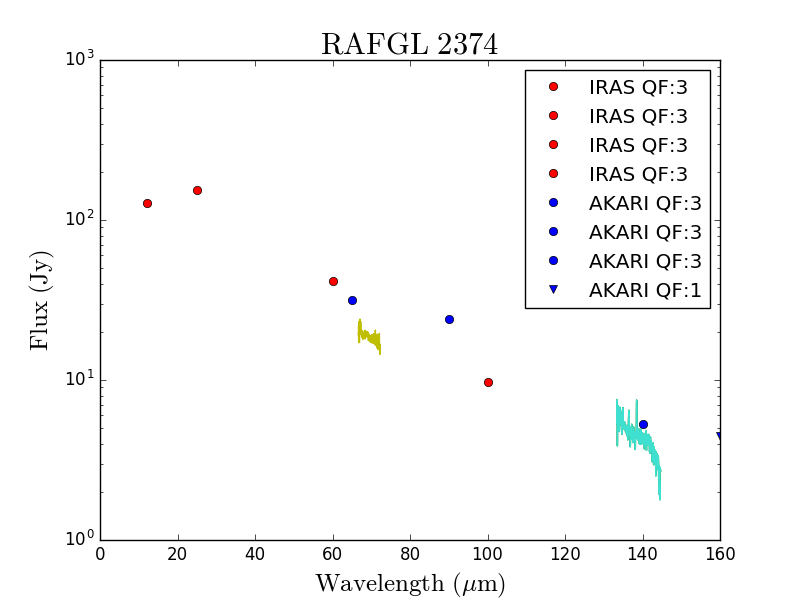
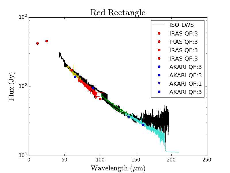
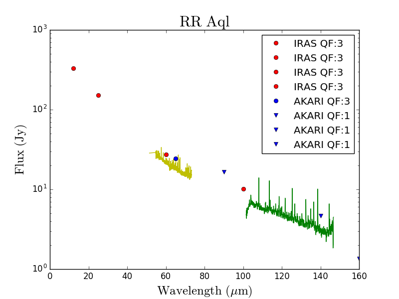
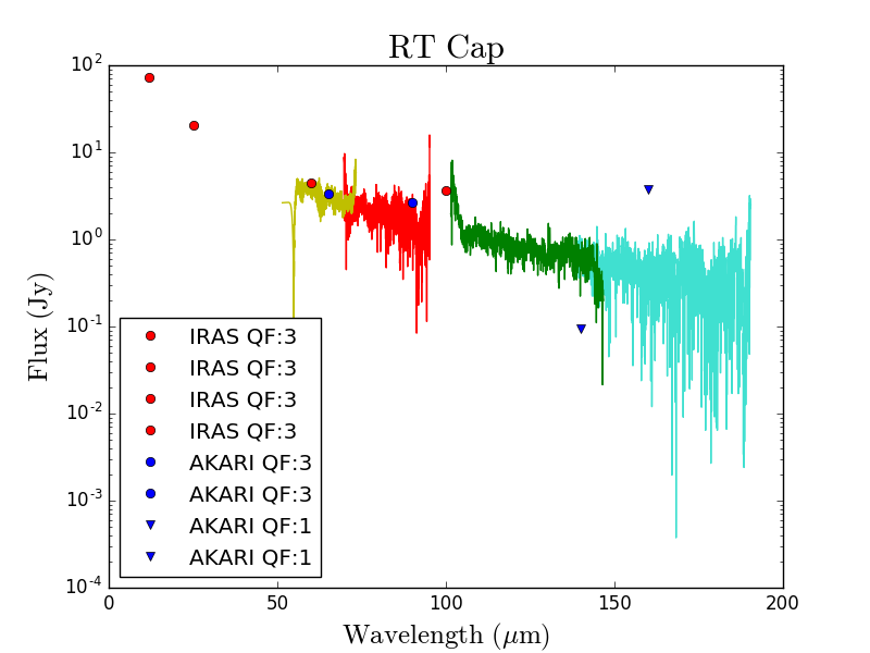
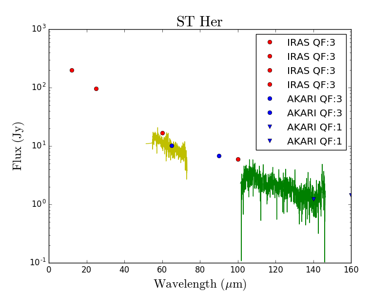
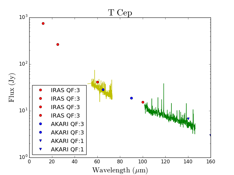
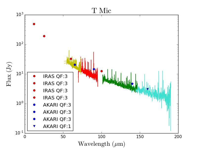
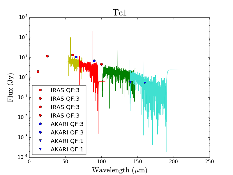
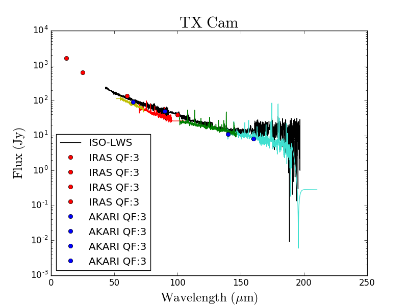
Figure 8: Continued.

Figure 8: Continued.

Figure 8: Continued.

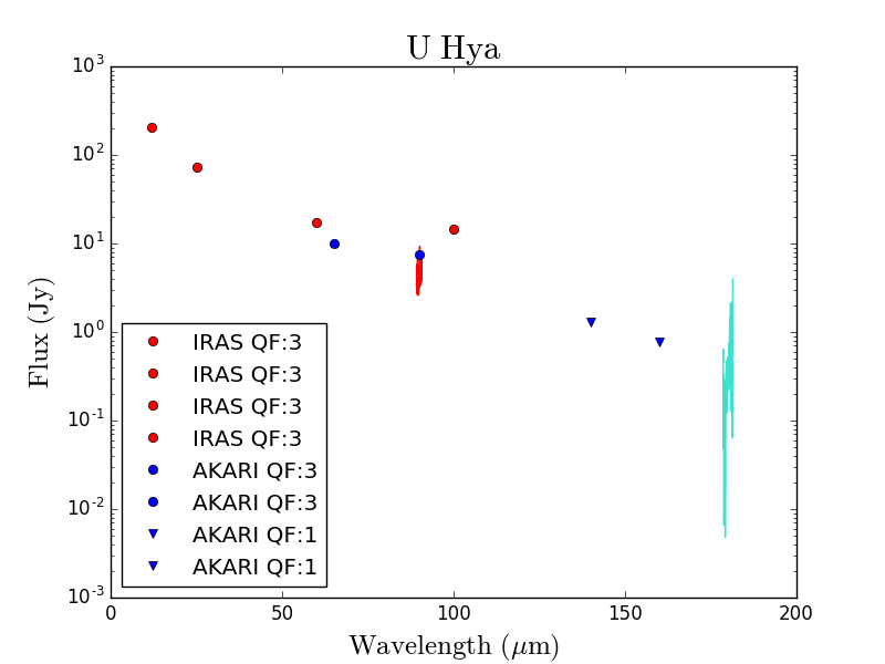
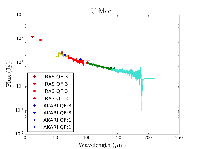
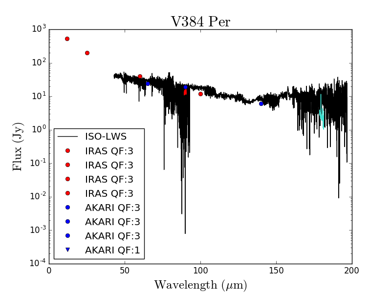
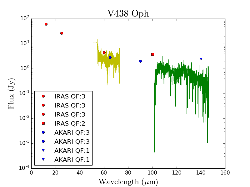
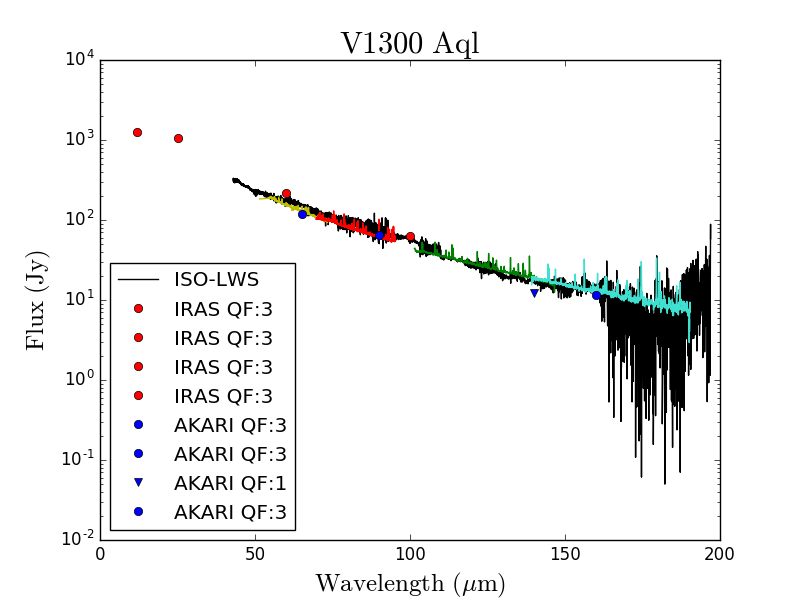
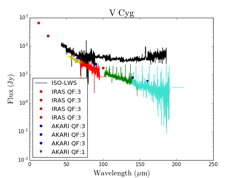
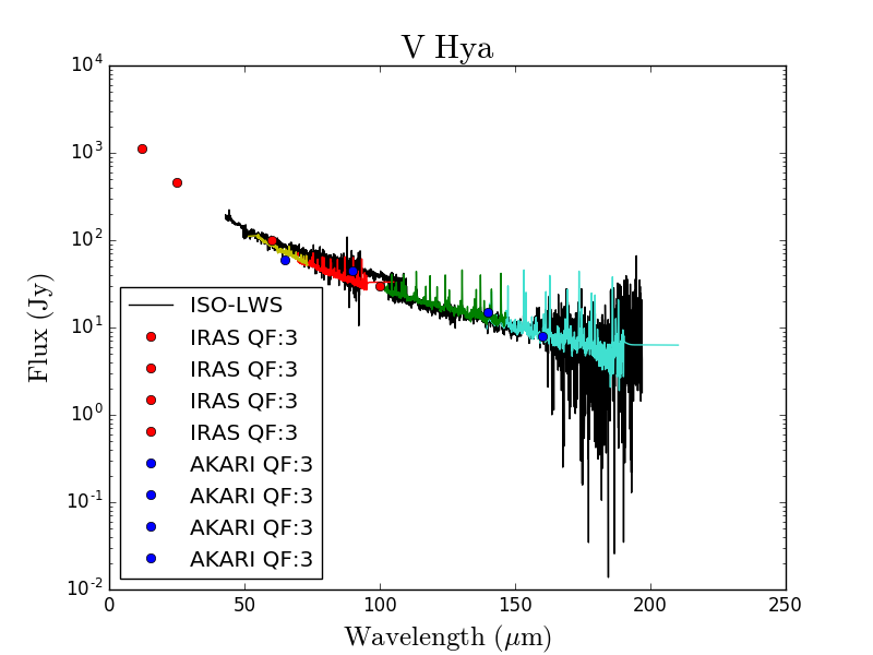
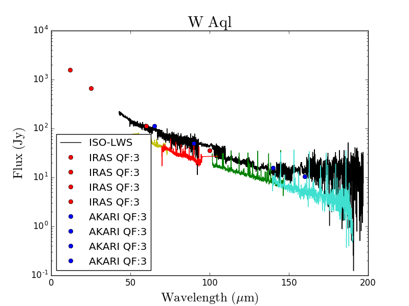
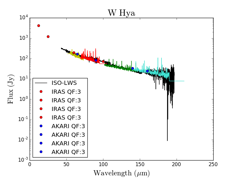
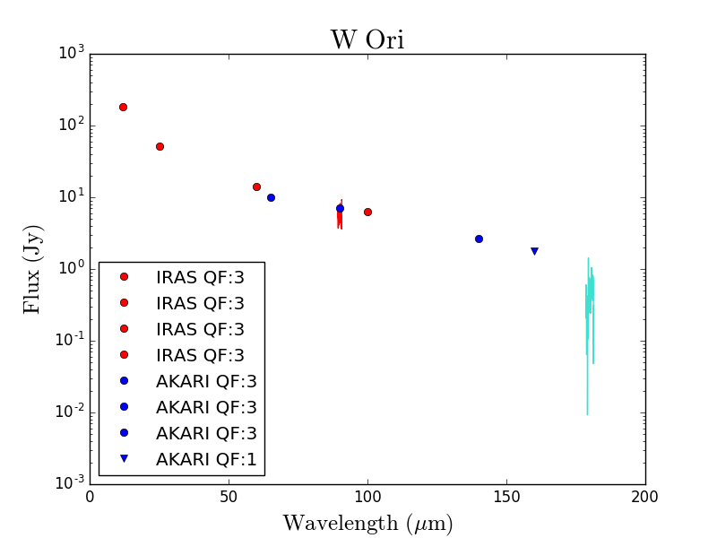
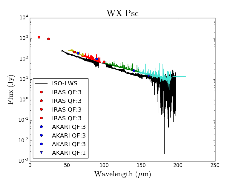
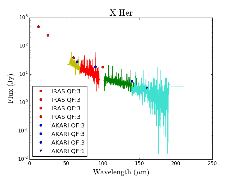
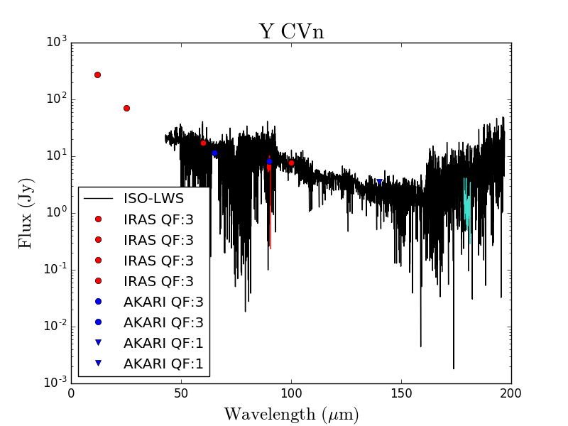
Figure 8: Continued.

Figure 8: Continued.

Figure 8: Continued.

Figure 8: Continued.

Figure 8: Continued.

Figure 8: Continued.

Figure 8: Continued.

Figure 8: Continued.

Figure 8: Continued.

Figure 8: Continued.

Figure 8: Continued.

Figure 8: Continued.

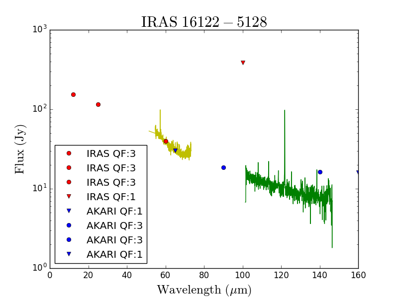
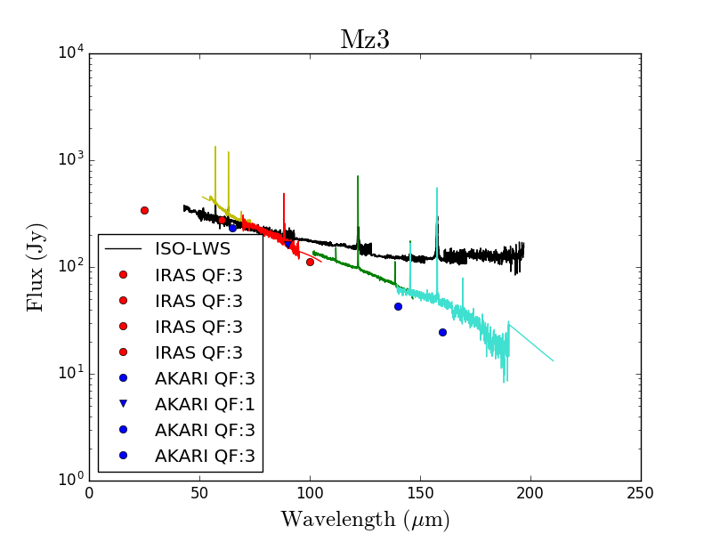
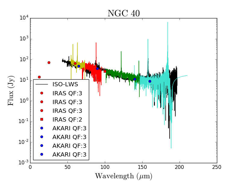
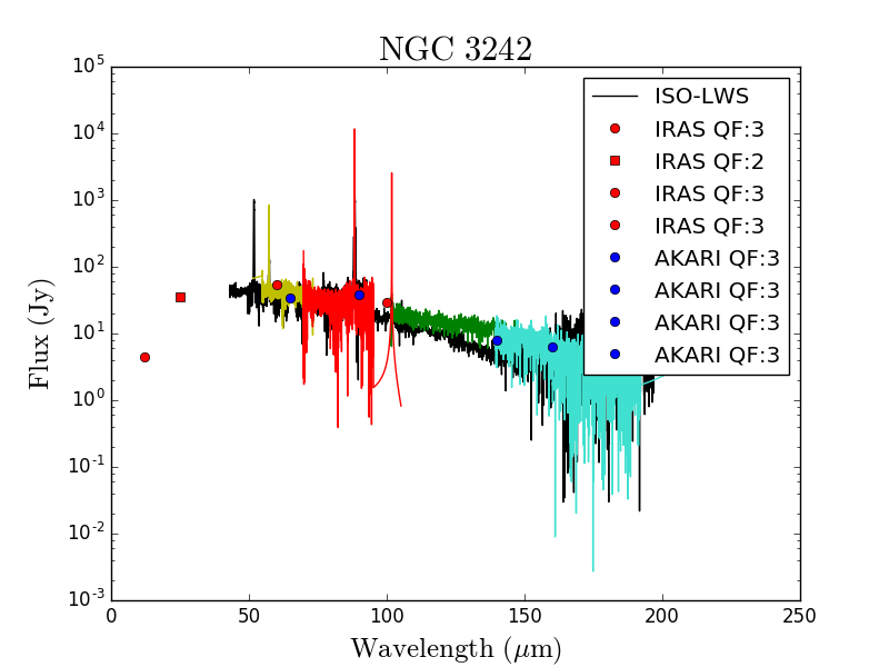
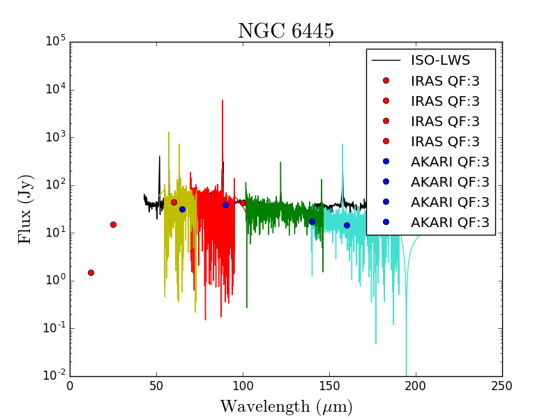
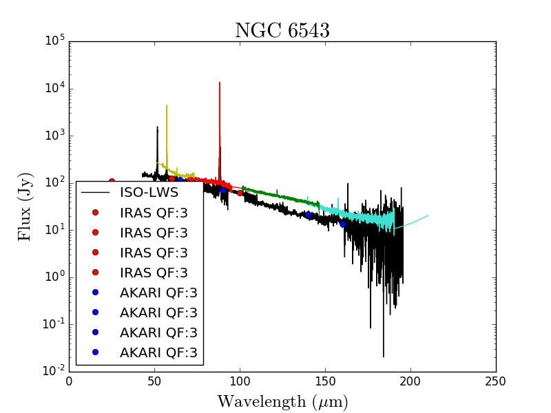
Figure 9: As in Fig. 8 but for extended objects after applying point source flux loss correction and extended 5x5 correction. IRAS 16122-5128 appears in THROES catalogue and in HSA as MGE 4218.

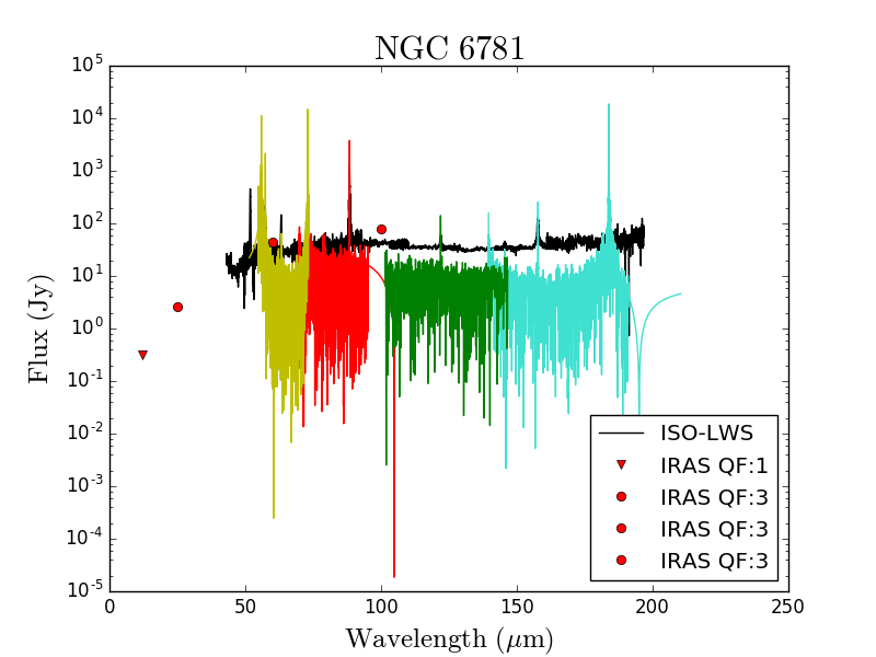
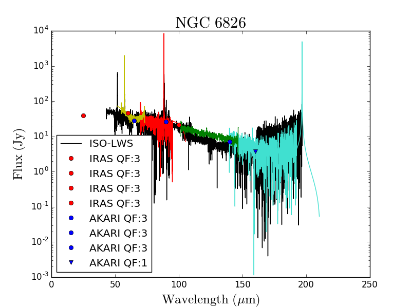
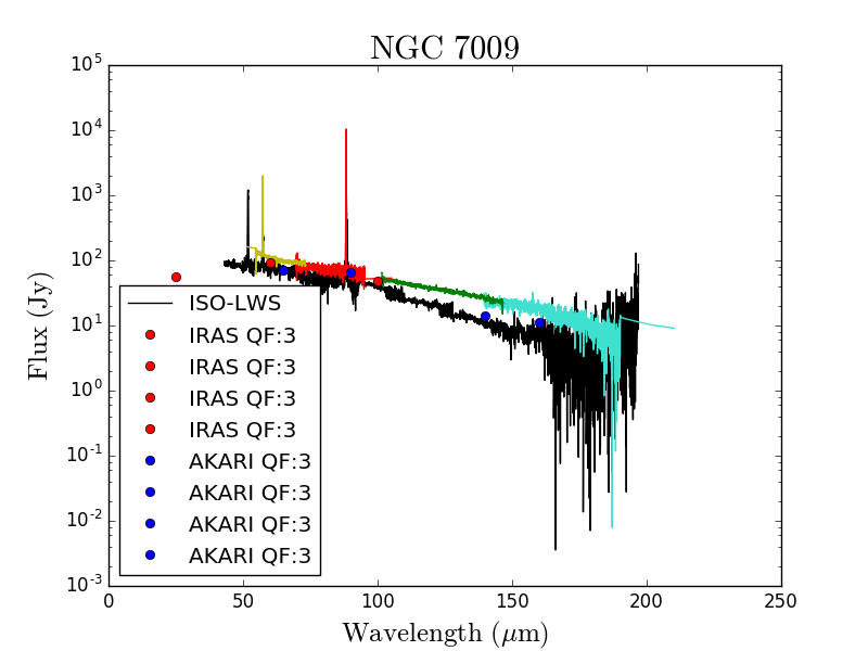
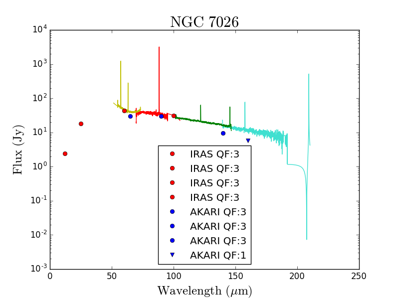
Figure 9: Continued.

Table 1: Basic information about all observations reprocessed in THROES. Column 1: Target name; Columns 2 and 3: Equatorial coordinates (J2000) in degrees; Columns 4, 5, and 6: Complementary data for each observation in IRAS, AKARI, or ISO; Column 7: Comments on complementary information about the PACS observations object: 1) Incomplete PACS wavelength coverage; 2) Mispointing (target not in the central spaxel); 3) Semi-extended object (size $\sim$3x3 central spaxels); 4) Extended object (size $\sim$5x5 spaxels); 5) Contamination in ISO data due to interstellar emission; 6) Faint source ($\leq$10 Jy at 60 $\mu$m); 7) Multi epochs observations. If the observation presents a complete spectral coverage in PACS wavelength range, is well pointed, Chop/Nod and the source is point-like and intense, there is no comment in the column (-); Column 8: ObsIds; Column 9: Date of observation.

Target name	RA(deg)	Dec(deg)	IRAS	AKARI	ISO	Comments	ObsIDs	Date
AC Her	277.5676	21.8668	Yes	Yes	Yes	1,6	1342208896	2010-11-13
AFGL 618	70.7236	36.1147	Yes	Yes	Yes	-	1342225838	2011-08-07
							1342225839	2011-08-07
							1342225840	2011-08-07
AFGL 2019	268.3282	-26.9436	Yes	Yes	No	1,6	1342252253	2012-10-05
AFGL 2403	292.6228	19.8447	Yes	Yes	No	1	1342245226	2012-05-01
AFGL 2513	302.3093	31.4291	Yes	Yes	No	-	1342270010	2013-04-14
							1342269936	2013-04-12
AFGL 2688	315.5781	36.6938	No	No	Yes	-	1342199233	2010-06-26
							1342199234	2010-06-26
							1342199235	2010-06-27
AFGL 3068	349.8016	17.1931	Yes	Yes	Yes	-	1342199417	2010-06-30
							1342199418	2010-06-30
							1342257635	2012-12-21
AFGL 3116	353.6152	43.5506	Yes	Yes	No	-	1342212512	2011-01-11
							1342212513	2011-01-11
AFGL 4106	155.8311	-59.5346	Yes	Yes	Yes	1	1342207818	2010-11-03
AFGL 4202	223.1012	-62.0721	Yes	Yes	No	1,6	1342250004	2012-08-21
AFGL 4259	301.5947	27.0362	Yes	Yes	No	1,6	1342244918	2012-04-24
AFGL 5379	266.0942	-31.9276	Yes	Yes	Yes	2	1342228537	2011-09-13
							1342228538	2011-09-13
AFGL 6815	259.5830	-32.4556	Yes	Yes	No	-	1342216629	2011-03-22
							1342216630	2011-03-22
AQ Sgr	293.5791	-16.3741	Yes	Yes	No	-	1342268751	2013-03-28
							1342268752	2013-03-28
BD +30 3639	293.6884	30.5163	Yes	Yes	Yes	3	1342220600	2011-05-04
							1342220601	2011-05-04
CIT 6	154.0094	30.5718	Yes	No	Yes	-	1342197799	2010-06-05
							1342197800	2010-06-05
CPD-568032	257.2536	-56.9133	Yes	Yes	Yes	-	1342228201	2011-09-06
							1342228202	2011-09-06
CPD-642939	219.2920	-64.8013	Yes	Yes	No	1,6	1342250006	2012-08-21
EP Aqr	326.6327	-2.2127	Yes	Yes	No	-	1342270639	2013-04-20
							1342270684	2013-04-21
G Her	247.1606	41.8816	Yes	Yes	No	1	1342247780	2012-07-09
HD 56126	109.0427	9.9966	Yes	Yes	Yes	-	1342220930	2011-04-30
							1342220931	2011-04-30
HD 161796	266.2311	50.0443	Yes	Yes	Yes	-	1342208881	2010-11-12
							1342208882	2010-11-12
HD 235858	337.2932	54.8517	Yes	Yes	No	-	1342196686	2010-05-18
							1342196687	2010-05-18
HD 331319	297.3731	31.4545	Yes	Yes	No	1	1342245232	2012-05-01
Hen 2-90	197.4009	-61.3266	Yes	Yes	Yes	1,5,6	1342248308	2012-07-16
Hen 2-113	224.9730	-54.3020	Yes	Yes	Yes	-	1342225142	2011-08-02
							1342225143	2011-08-02
							1342249211	2012-08-07
Hen 3-401	154.8852	-60.2248	Yes	Yes	No	-	1342225588	2011-08-03
							1342225589	2011-08-03
Hen 3-1475	266.3090	-17.9462	Yes	Yes	Yes	-	1342229719	2011-09-24
							1342229720	2011-09-24
IC 418	81.8675	-12.6973	Yes	No	Yes	3	1342265942	2013-03-04
							1342265943	2013-03-04
IRAS 07027-7934	104.8599	-79.6463	Yes	Yes	Yes	1,6	1342245248	2012-05-02
IRAS 08011-3627	120.7568	-36.5966	Yes	Yes	No	-	1342210381	2010-11-27
							1342256781	2012-12-04
							1342256782	2012-12-04
IRAS 08544-4431	134.0591	-44.7196	Yes	Yes	No	-	1342245956	2012-05-21
							1342245957	2012-05-21
IRAS 09256-6324	141.7220	-63.6302	Yes	Yes	No	-	1342210386	2010-11-27
							1342248357	2012-07-20
							1342248358	2012-07-20
IRAS 09371+1212	144.9749	11.9814	Yes	Yes	No	-	1342245647	2012-05-12
							1342245648	2012-05-12
IRAS 09425-6040	146.0066	-60.9072	Yes	Yes	No	-	1342225563	2011-07-25
							1342225564	2011-07-25
IRAS 10456-5712	161.91	-57.4674	Yes	Yes	No	-	1342211823	2010-12-28
							1342248928	2012-07-31
							1342248929	2012-07-31
IRAS 13428-6232	206.5854	-62.8000	Yes	Yes	No	2	1342212212	2010-12-31
							1342212213	2010-12-31
IRAS 15194-5115	230.7704	-51.4330	Yes	Yes	Yes	-	1342215685	2011-03-10
							1342215686	2011-03-10
IRAS 16122-5128	244.0190	-51.5989	Yes	Yes	No	1	1342240167	2012-02-18
IRAS 16279-4757	247.9087	-48.0677	Yes	Yes	No	2	1342228203	2011-09-06
							1342228204	2011-09-06
IRAS 16342-3814	249.417	-38.3380	Yes	Yes	Yes	-	1342216627	2011-03-22
							1342216628	2011-03-22
IRAS 16594-4656	255.7917	-47.0076	Yes	Yes	Yes	5	1342228414	2011-09-10
							1342228415	2011-09-10
IRAS 17010-3840	256.1179	-38.7396	Yes	Yes	No	1,6	1342216176	2011-03-16
IRAS 17251-2821	262.0770	-28.3991	Yes	Yes	No	1,6	1342228535	2011-09-13
IRAS 17276-2846	262.7012	-28.8172	Yes	Yes	No	1,6	1342228536	2011-09-13
IRAS 17323-2424	263.8583	-24.4422	Yes	Yes	No	1,6	1342228532	2011-09-13
IRAS 17347-3139	264.5054	-31.6827	Yes	No	No	2	1342229696	2011-09-24
							1342229697	2011-09-24
IRAS 17521-2938	268.8404	-29.6536	Yes	No	No	1,6	1342229802	2011-09-27
IRAS 18433-0228	281.4800	-2.4189	Yes	No	No	1	1342231743	2011-11-01
IRAS 18488-0107	282.8592	-1.0645	Yes	No	No	-	1342268791	2013-03-30
							1342268792	2013-03-30
IRAS 19067+0811	287.2845	8.2770	Yes	Yes	No	-	1342268797	2013-03-31
							1342268798	2013-03-31
IRAS 19306+1407	293.2295	14.2269	Yes	Yes	No	1,6	1342244921	2012-04-24
IRAS 19474-0744	297.5264	-7.6145	Yes	Yes	No	-	1342268638	2013-03-25
							1342268449	2013-03-26
IRAS 20000+3239	300.4980	32.7924	Yes	Yes	No	-	1342270612	2013-04-18
							1342270344	2013-04-17
IRAS 20038-2722	301.7301	-27.2249	Yes	Yes	No	-	1342268730	2013-03-29
							1342268569	2013-03-27
IRAS 21282+5050	322.4934	51.0666	Yes	Yes	Yes	5	1342223375	2011-06-30
							1342220741	2011-05-12
IRAS 21554+6204	329.2424	62.3121	Yes	Yes	No	1,6	1342245813	2012-05-15
							1342247150	2012-06-20
IRAS 22036+5306	331.3761	53.3591	Yes	Yes	Yes	5	1342221882	2011-05-29
							1342221883	2011-05-29
IRC +10216	146.9892	13.2787	Yes	No	No	1,7	1342245395	2012-05-05
							1342221889	2011-05-29
							1342253754	2012-10-21
							1342256262	2012-11-30
IRC -10529	302.6142	-6.2710	Yes	Yes	Yes	2	1342208931	2010-11-14
							1342208932	2010-11-14
IRC +50137	77.831	52.8758	Yes	Yes	No	1	1342249315	2012-08-10
$\chi$ Cyg	297.6413	32.9140	Yes	Yes	Yes	-	1342198176	2010-06-02
							1342198177	2010-06-02
MGE 4602	271.1620	-20.6242	Yes	Yes	No	1,6	1342243506	2012-03-24
MWC 922	275.3162	-13.0241	Yes	Yes	Yes	5	1342229805	2011-09-27
							1342229806	2011-09-27
Mz 3	244.3058	-51.9862	Yes	Yes	Yes	4	1342243109	2012-03-21
							1342243110	2012-03-21
NGC 40	3.2542	72.5219	Yes	Yes	Yes	4,6	1342236879	2012-01-08
							1342236880	2012-01-08
NGC 2392	112.2948	20.9118	Yes	Yes	No	6	1342229792	2011-09-26
							1342229816	2011-09-27
NGC 3242	156.1920	-18.6411	Yes	Yes	Yes	4,6	1342232278	2011-11-12
							1342232279	2011-11-12
NGC 6302	258.4342	-37.1044	Yes	Yes	Yes	2	1342230150	2011-10-05
							1342230151	2011-10-05
NGC 6445	267.3133	-20.0095	Yes	Yes	Yes	4,6	1342242440	2012-03-26
							1342242441	2012-03-26
NGC 6537	271.3045	-19.8430	No	Yes	Yes	3,5	1342231322	2011-10-22
							1342231323	2011-10-22
NGC 6543	269.6385	66.6330	No	Yes	Yes	4	1342238388	2012-01-29
							1342238389	2012-01-29
							1342212264	2011-01-02
NGC 6543 WKnot	269.5722	66.6356	No	No	No	-	1342235679	2011-12-27
							1342235680	2011-12-27
NGC 6720	283.3961	33.0291	Yes	Yes	Yes	1,6	1342208920	2010-11-14
NGC 6720 OFFCenter	283.3937	33.0326	Yes	Yes	Yes	-	1342233716	2011-12-07
							1342233717	2011-12-07
NGC 6781	289.6170	6.5386	Yes	No	Yes	4,6	1342230999	2011-10-14
							1342231000	2011-10-14
NGC 6781 Rim	289.6313	6.5388	No	No	No	-	1342231001	2011-10-15
							1342231002	2011-10-15
NGC 6826	296.2006	50.5250	Yes	Yes	Yes	3,6	1342238926	2012-02-10
							1342238927	2012-02-10
NGC 6826 Rim	296.2207	50.5290	No	No	No	-	1342235850	2011-12-31
							1342235851	2011-12-31
NGC 7009	316.0450	-11.3635	Yes	Yes	Yes	4	1342232300	2011-11-13
							1342232301	2011-11-13
NGC 7026	316.5773	47.8519	Yes	Yes	No	3	1342234268	2011-12-06
							1342234269	2011-12-06
NML Cyg	311.606	40.1165	No	Yes	Yes	-	1342198174	2010-06-02
							1342198175	2010-06-02
NML Tau	58.3701	11.4062	Yes	Yes	Yes	-	1342203679	2010-08-28
							1342203680	2010-08-28
							1342203681	2010-08-28
OH 21.5+0.5	277.1316	-9.9696	No	No	No	2,7	1342242438	2012-03-26
							1342268778	2013-03-29
							1342268748	2013-03-30
OH 26.5+0.6	279.3852	-5.3998	Yes	Yes	Yes	5	1342207776	2010-10-31
							1342207777	2010-10-31
OH 30.1-0.7	282.1746	-2.8411	Yes	Yes	No	-	1342216207	2011-03-04
							1342269304	2013-04-03
							1342269305	2013-04-03
OH 30.7+0.4	281.5241	-1.9881	Yes	No	No	6	1342268789	2013-03-30
							1342268790	2013-03-30
OH 32.8-0.3	283.0924	-0.2371	Yes	No	Yes	5,7	1342209738	2010-11-07
							1342268793	2013-03-30
							1342268794	2013-03-30
OH 104.91+2.41	334.8645	59.8560	Yes	Yes	Yes	1	1342212261	2011-01-01
OH 231.8+4.2	115.5701	-14.7144	Yes	Yes	No	-	1342196694	2010-05-19
							1342196695	2010-05-19
$o$ Cet	34.8366	-2.9776	Yes	Yes	No	-	1342213286	2011-01-25
							1342213287	2011-01-25
$\pi$ Gru	335.6842	-45.9479	Yes	Yes	Yes	-	1342210397	2010-11-28
							1342210398	2010-11-28
R Aql	286.5927	8.2300	Yes	Yes	Yes	1,5	1342243900	2012-04-08
R Cas	359.6036	51.3888	Yes	Yes	Yes	-	1342212576	2011-01-12
							1342212577	2011-01-12
R Dor	69.1899	-62.0771	Yes	Yes	Yes	3	1342197794	2010-06-05
							1342197795	2010-06-05
R Lep	74.9014	-14.8062	Yes	Yes	No	1,6	1342249509	2012-08-14
RAFGL 2374	290.4021	9.4656	Yes	Yes	No	1,6	1342244920	2012-04-24
Red Rectangle	94.9925	-10.6374	Yes	Yes	Yes	-	1342220928	2011-04-30
							1342220929	2011-04-30
RR Aql	299.4002	-1.8864	Yes	Yes	No	1	1342269414	2013-04-05
RT Cap	304.2772	-21.3179	Yes	Yes	No	6	1342269308	2013-04-03
							1342269355	2013-04-04
S Aur	81.7810	34.1496	Yes	Yes	No	1,6	1342250896	2012-09-11
ST Her	237.6942	48.4830	Yes	Yes	No	1,6	1342247537	2012-06-30
T Cep	317.3824	68.4908	Yes	Yes	No	1	1342246557	2012-06-01
T Mic	306.9799	-28.2610	Yes	Yes	No	-	1342268729	2013-03-29
							1342268788	2013-03-30
							1342269458	2013-04-06
Tc 1	266.3970	-46.0899	Yes	Yes	No	6	1342231319	2011-10-22
							1342231320	2011-10-22
TX Cam	75.2099	56.1812	Yes	Yes	Yes	3	1342225855	2011-08-08
							1342225856	2011-08-08
U Hya	159.3886	-13.3845	Yes	Yes	No	1,6	1342256947	2012-12-11
U Mon	112.6977	-9.7768	Yes	Yes	No	-	1342206993	2010-10-23
							1342245243	2012-05-02
							1342245244	2012-05-02
V384 Per	51.6229	47.5301	Yes	Yes	Yes	1,6	1342250572	2012-09-04
V438 Oph	258.6657	11.0694	Yes	Yes	No	1,6	1342252326	2012-10-07
V1300 Aql	302.6161	-6.2704	Yes	Yes	Yes	-	1342269516	2013-04-07
							1342269910	2013-04-11
V Cyg	310.3261	48.1413	Yes	Yes	Yes	5	1342208939	2010-11-15
							1342208940	2010-11-15
V Hya	162.9052	-21.2500	Yes	Yes	Yes	-	1342197790	2010-06-05
							1342197791	2010-06-05
W Aql	288.8476	-7.0471	Yes	Yes	Yes	-	1342209731	2010-11-06
							1342209732	2010-11-07
W Hya	207.2583	-28.3676	Yes	Yes	Yes	-	1342212604	2011-01-14
							1342223808	2011-07-09
W Ori	76.3488	1.1776	Yes	Yes	No	1,6	1342249503	2012-08-14
WX Psc	16.6082	12.5980	Yes	Yes	Yes	-	1342202121	2010-07-28
							1342202122	2010-07-28
X Her	240.6632	47.2403	Yes	Yes	No	-	1342197802	2010-06-05
							1342197803	2010-06-05
							1342202120	2010-07-28
Y CVn	191.2826	45.4402	Yes	Yes	Yes	1,6	1342254305	2012-11-02

Table 1: Continued.

Table 2: . Photometric data of THROES targets. Target name (Col. 1), as it appears in HSA, galactic coordinates (Cols. 2 and 3), IRAS (100 $\mu$m) and AKARI (160 $\mu$m) photometric data (Cols. 4 and 5), and PACS synthetic photometry at 100 and 160 $\mu$m (Cols. 6 and 7)

Target name	b(deg)	l(deg)	IRAS100 (Jy)	AKARI160 (Jy)	PACSIRAS100 (Jy)	PACSAKARI160 (Jy)
AC Her	14.2415	50.4928	8.0	¡3.2	-	-
AFGL 618	-6.5275	166.4460	340.0	111.7	859.0	195.9
AFGL 2019	-0.4324	2.5826	¡227.0	48.6	-	-
AFGL 2403	0.7353	54.9494	¡31.3	¡10.1	-	-
AFGL 2513	-0.8653	69.3522	20.8	¡5.8	10.7	3.9
AFGL 2688	-6.5032	80.1675	¡863.0	-	1969.1	467.8
AFGL 3068	-40.3540	93.5266	73.7	24.4	102.0	34.3
AFGL 3116	-17.1467	108.4549	35.5	10.9	46.8	14.9
AFGL 4106	-1.8789	285.1439	181.0	60.1	-	-
AFGL 4202	-2.4514	316.5887	¡75.3	¡6.5	-	-
AFGL 4259	-2.7141	65.3167	7.5	¡2.6	-	-
AFGL 5379	-1.3330	357.3084	406.0	¡31.2	-	-
AFGL 6815	2.9842	353.8442	82.4	¡18.37	120.0	40.3
AQ Sgr	-16.7007	22.7377	5.9	¡0.5	1.3	0.4
BD +30 3639	5.0194	64.7853	70.1	¡23.1	70.6	21.0
CIT 6	55.9641	197.7148	86.1	-	83.5	24.2
CPD-568032	-9.9082	332.9152	91.7	29.4	106.2	26.7
CPD-642939	-4.2026	313.8867	20.6	¡4.7	-	-
EP Aqr	-39.2603	54.2000	16.4	¡4.9	15.0	4.7
G Her	43.7146	66.1579	6.6	¡0.1	-	-
HD 56126	9.9947	206.7457	18.7	¡3.8	20.5	6.0
HD 161796	30.8696	77.1331	48.7	10.7	56.1	8.0
HD 235858	-2.5181	103.3488	41.0	8.5	34.0	10.0
HD 331319	2.7327	67.1633	14.8	¡4.1	-	-
Hen 2-90	1.4683	305.1099	¡50.2	¡11.1	-	-
Hen 2-113	3.9885	321.0483	71.3	20.9	90.7	26.0
Hen 3-401	-2.7162	285.1194	41.5	16.6	45.2	15.7
Hen 3-1475	5.7788	9.3644	33.4	12.1	36.2	9.7
IC 418	-24.2837	215.2120	31.2	-	29.1	9.5
IRAS 07027-7934	-26.2939	291.3749	13.6	¡4.4	-	-
IRAS 08011-3627	-2.9959	253.0207	12.0	¡4.7	13.6	4.6
IRAS 08544-4431	0.3864	265.5011	¡28.4	¡3.2	29.3	11.5
IRAS 09256-6324	-9.2362	282.4206	13.5	¡5.3	15.6	7.1
IRAS 09371+1212	42.7271	221.8893	28.2	¡11.6	32.7	15.5
IRAS 09425-6040	-5.8842	282.0386	5.1	¡1.3	7.5	1.8
IRAS 10456-5712	1.4921	286.8707	10.9	¡5.1	15.6	5.8
IRAS 13428-6232	-0.5939	309.1588	¡186.0	36.9	-	-
IRAS 15194-5115	4.6593	325.5339	51.0	15.0	37.0	11.4
IRAS 16122-5128	-0.6095	331.8689	¡387.0	¡16.1	-	-
IRAS 16279-4757	0.0851	336.1433	¡265.0	-	-	-
IRAS 16342-3814	5.8464	344.0739	139.0	43.2	193.9	65.4
IRAS 16594-4656	-3.2887	340.3924	34.4	¡10.6	45.7	10.8
IRAS 17010-3840	1.5481	347.1050	¡50.1	¡6.3	-	-
IRAS 17251-2821	3.4922	358.4142	¡19.9	-	-	-
IRAS 17276-2846	2.8046	358.3664	¡30.0	-	-	-
IRAS 17323-2424	4.3084	2.6112	¡13.5	¡0.7	-	-
IRAS 17347-3139	-0.0557	356.8018	¡249.0	-	-	-
IRAS 17521-2938	-2.1916	0.4718	¡110.0	-	-	-
IRAS 18433-0228	0.1239	30.1503	¡240.0	-	-	-
IRAS 18488-0107	-0.4851	31.9844	72.8	-	20.9	6.9
IRAS 19067+0811	-0.1323	42.3093	¡91.1	-	12.4	2.4
IRAS 19306+1407	-2.4774	50.3034	10.0	¡7.6	-	-
IRAS 19474-0744	-16.4859	32.7232	17.2	¡3.2	20.8	6.5
IRAS 20000+3239	1.1609	69.6792	¡43.1	-	12.0	3.4
IRAS 20038-2722	-27.6822	14.7708	13.6	¡0.8	9.8	3.3
IRAS 21282+5050	-0.1178	93.9871	15.0	¡3.7	16.6	7.2
IRAS 21554+6204	5.9916	104.1301	15.6	¡3.3	-	-
IRAS 22036+5306	-1.8353	99.6333	50.7	20.3	66.1	21.2
IRC +10216	45.0604	221.4467	922.0	-	-	-
IRC -10529	-20.4151	36.3565	63.7	11.4	-	-
IRC +50137	7.8349	156.4379	23.0	6.6	-	-
$\chi$ Cyg	3.2762	68.5386	17.7	¡6.9	24.2	6.8
MGE 4602	0.4734	9.3523	¡50.0	¡14.0	-	-
Mz 3	-1.0113	331.7275	113.0	24.7	77.5	28.3
NGC 40	9.8680	120.0162	27.5	9.1	11.5	4.8
NGC 2392	17.4002	197.8784	16.1	¡3.3	-	-
NGC 3242	32.0509	261.0499	29.6	6.4	15.4	3.6
NGC 6302	1.0558	349.5075	537.0	201.7	-	-
NGC 6445	3.9051	8.0758	43.2	14.6	13.4	3.5
NGC 6537	0.7395	10.0989	166.0	¡85.5	155.4	70.9
NGC 6543	29.9548	96.4680	60.9	13.9	48.5	13.0
NGC 6543 WKnot	29.9810	96.4712	-	-	-	-
NGC 6720	13.9782	63.1700	54.6	20.6	-	-
NGC 6720 OFFcenter	13.9814	63.1725	54.6	20.6	-	-
NGC 6781	-2.9878	41.8407	77.0	-	0.6	1.6
NGC 6781 Rim	-3.0000	41.8475	77.0	-	-	-
NGC 6826	12.7923	83.5616	21.3	¡3.7	11.7	5.8
NGC 6826 Rim	12.7828	83.5713	-	-	-	-
NGC 7009	-34.5713	37.7621	48.1	11.3	29.0	8.6
NGC 7026	0.3753	89.0020	30.9	¡5.8	17.8	1.7
NML Cyg	-1.9208	80.7982	¡334.0	100.1	400.0	109.2
NML Tau	-31.4120	177.9545	103.0	27.4	131.1	22.9
OH 21.5+0.5	0.4893	21.4588	¡319.0	-	-	-
OH 26.5+0.6	0.6179	26.5434	¡311.0	¡30.25	181.0	33.5
OH 30.1-0.7	-0.6862	30.0911	¡807.0	-	93.6	15.0
OH 30.7+0.4	0.2813	30.5537	290.0	-	6.9	12.7
OH 32.8-0.3	-0.3154	32.8271	¡583.0	-	68.6	14.0
OH 104.91+2.41	2.4134	104.9083	35.0	7.8	-	-
OH 231.8+4.2	4.2196	231.8354	294.0	98.9	586.2	198.0
$o$ Cet	-57.9827	167.7549	88.4	16.1	74.3	18.5
$\pi$ Gru	-55.1638	350.2822	23.3	¡5.5	18.4	6.0
R Aql	0.4539	41.9524	¡83.1	-	-	-
R Cas	-10.6191	114.5608	38.8	9.5	29.6	10.5
R Dor	-39.3424	272.6713	83.4	25.5	92.8	33.2
R Lep	-31.3270	214.3244	9.1	¡0.5	-	-
RAFGL 2374	-2.3064	44.7947	9.8	¡4.5	-	-
Red Rectangle	-11.7648	218.9680	66.2	¡28.0	88.4	35.0
RR Aql	-15.5601	38.9171	10.1	¡1.4	-	-
RT Cap	-27.9386	21.9411	3.6	¡3.8	2.2	0.6
S Aur	-0.5112	173.4866	11.6	¡0.7	-	-
ST Her	49.4432	76.9788	6.0	¡1.4	-	-
T Cep	13.8449	104.8050	15.3	¡3.0	-	-
T Mic	-32.4287	15.1857	12.7	¡3.1	10.4	3.2
Tc 1	-8.8349	345.2375	4.7	¡0.5	2.0	1.0
U Hya	38.0741	259.9663	14.5	¡0.8	-	-
U Mon	4.1536	226.1413	9.5	-	12.0	4.9
V384 Per	-7.5975	148.1771	11.9	-	-	-
V438 Oph	26.4554	32.1306	3.7	-	-	-
V1300 Aql	-20.4165	36.3580	63.7	11.4	72.7	17.5
V Cyg	3.7667	86.5361	17.2	¡6.0	13.3	5.2
V Hya	33.6014	268.9648	29.9	8.0	33.9	9.6
W Aql	-8.5161	29.3389	36.0	10.6	26.6	7.6
W Hya	32.8108	318.0223	72.2	24.3	72.3	26.6
W Ori	-22.8179	199.0092	6.27	¡1.8	-	-
WX Psc	-50.1074	128.6416	72.1	¡15.0	77.5	19.8
X Her	47.7855	74.4639	18.3	¡3.3	9.5	3.6
Y CVn	71.6450	126.4472	7.8	-	-	-

Table 2: Continued.