The pressure tensor across a liquid-vapour interface

Abstract

Inhomogeneous fluids exhibit physical properties that are neither uniform nor isotropic. The pressure tensor is a case in point, key to the mechanical description of the interfacial region. Kirkwood and Buff, and later Irving and Kirkwood, obtained a formal treatment based on the analysis of the pressure across a planar surface  [J.G. Kirkwood and F.P. Buff, J. Chem. Phys., 17(3), (1949), J.H. Irving and J.G. Kirkwood, J. Chem. Phys. 18, 817 (1950)]. We propose a generalisation of Irving and Kirkwood’s argument to fluctuating, non-planar surfaces and obtain an expression for the pressure tensor that is not smeared by thermal fluctuations at the molecular scale and corresponding capillary waves  [F.P. Buff, R.A. Lovett, and F.H. Stillinger, Jr., Phys. Rev. Lett. 15, 621 (1965)]. We observe the emergence of surface tension, defined as an excess tangential stress, acting exactly across the dividing surface at the sharpest molecular resolution. The new statistical mechanical expressions extend current treatments to fluctuating inhomogeneous systems far from equilibrium.

I Introduction

Inhomogeneous systems are characterised by an interface, across which physical quantities vary sharply, over a length scale of a few molecular diameters (Rowlinson and Widom, 2002). Thermally induced fluctuations of the interface in the form of capillary waves smooth out the transition of properties across the interface. Although capillary wave behaviour has been observed experimentally (Sanyal et al., 1991; Tidswell et al., 1991), analysis of the interfacial structure at the sharpest molecular resolution is difficult as a result of these fluctuations. Capillary wave theory (CWT), introduced by Buff et al. (Buff et al., 1965; Evans, 1979), accounts for these by assuming the existence of an intrinsic surface $\displaystyle\textstyle\xi\left(\mathbf{x}\right)$, where $\displaystyle\mathbf{x}$ is a vector in the coordinate system parallel to the surface. This function acts as an instantaneous boundary between fluid phases, against which statistical averages are computed, e.g. the intrinsic density profile,

$$\tilde{\rho}\left(z+\xi\right)=\frac{1}{A}\sum\limits_{i=1}^{N}\,\left<\delta\left(z+\xi\left(\mathbf{x}_{i}\right)-z_{i}\right)\right>$$ (1)

where $\displaystyle\left(\mathbf{x}_{i},z_{i}\right)=\left(x_{i},y_{i},z_{i}\right)$ are the atom positions and $\displaystyle A=L_{x}L_{y}$ is the transverse area. In its original form (Buff et al., 1965), CWT sees the interface at the largest wavelength as a step function, whose local position is described by a Gaussian distribution $\displaystyle P\left(\xi\right)\propto\exp(-(\xi-\left<\xi\right>)^{2}/2w^{2})$. The square width $\displaystyle w^{2}$ characterises the correlation length of the surface fluctuations and is known to have the taxing property of, in absence of an external field, diverging in the thermodynamic limit (Percus, 1986; Fernández et al., 2013). The connection with the singlet density $\displaystyle\rho\left(z\right)$ is often accomplished by ignoring the coupling between capillary wave fluctuations and interfacial structure, resulting in a congruent fluctuation of the intrinsic profile. The mean density profile is then obtained from the convolution over the capillary waves, $\displaystyle\textstyle\rho\left(z\right)=\int\,\mathrm{d}\xi\,\tilde{\rho}\left(z-\xi\right)\,P\left(\xi\right)$ (Müller and Münster, 2005).

Among the different results reported previously, the interfacial Hamiltonian approach (e.g. Refs Die, 1999; Par, 2000; H$\displaystyle\ddot{\rm o}$fling and Dietrich, 2015; Yatsyshin, Parry, and Kalliadasis, 2016) gives useful information on the wavenumber dependence of surface tension but relies on various phenomenological parameters which are not known before hand. Further recently, there has been a renewed interest in the analysis of the pressure tensor in inhomogeneous systems, notably by Sega et al. in (Sega, Fábián, and Jedlovszky, 2015) for a Lennard-Jones (LJ) fluid and in (Sega et al., 2016) for molecular liquids. In these works the authors performed a deconvolution of the pressure tensor from the fluctuations in the interface position, thereby obtaining its intrinsic counterpart. The intrinsic profile of single particle properties is trivially obtained by appropriate weighting of the sum in Eq. (1), $\displaystyle\textstyle\tilde{\rho}_{w}(z)=\sum_{i}\,\left<w_{i}\delta(z+\xi\left(\mathbf{x}_{i}\right)-z_{i})\right>/A$, where $\displaystyle w_{i}$ is an arbitrary atomic weight. In contrast, the potential component of the pressure, $\displaystyle\mathbf{P}^{c}(\mathbf{r})$, is not easily defined due to the intermolecular interactions (Todd, Evans, and Daivis, 1995). For a pairwise potential, $\displaystyle\textstyle\mathbf{P}^{c}(\mathbf{r})=1/2\sum_{i\neq j}\,\left<\mathbf{F}_{ij}\int_{C_{ij}}\,\mathrm{d}\mathbf{l}\,\delta(\mathbf{l}-\mathbf{r})\right>$ where $\displaystyle\mathbf{F}_{ij}$ is the force between the pair of atoms, and $\displaystyle C_{ij}$ is the path of the line integral connecting atom $\displaystyle i$ and $\displaystyle j$.

There is no unique way of defining $\displaystyle C_{ij}$, and so there is also no unique way of determining which atom pairs contribute to the force across a given surface element (Baus and Lovett, 1990). Irving-Kirkwood (IK) convention (Irving and Kirkwood, 1950) stipulates that the force between two atoms is said to be across if the vector connecting the centres of mass of the two atoms intersects the surface element. The alternative Harasima (H) contour (Harasima, 1958) breaks the line connecting a pair of atoms into two mutually orthogonal paths. For planar interfaces, the H representation is seen as particularly convenient, because by construction, the transverse contribution of each pair of particles becomes path independent (Sega, Fábián, and Jedlovszky, 2015); on the other hand, there are always two possible H contours connecting a pair of particles, first transverse and then normal $\displaystyle\uparrow\circ\rightarrow$, and vice versa, $\displaystyle\rightarrow\circ\uparrow$. In the presence of an interface, this distinction is important, because it defines the position where the contribution to total pressure is accounted for. This is usually mitigated by equally partitioning the contribution at each particle’s location but it does not resolve the fundamental ambiguity.

Furthermore, it is also recognised that the normal component of this contour is known to not be physically meaningful (Sega, Fábián, and Jedlovszky, 2015; Schofield and Henderson, 1982). This additional conceptual difficulty is usually reconciled by arguing that mechanical stability, $\displaystyle\textstyle\mathbf{\nabla}\cdot\mathbf{P}=0$, requires uniformity of the normal pressure across the system. As it stands, this assumption can only hold under equilibrium conditions. Gradients in mass, momentum and energy will generate thermodynamic fluxes that change the liquid structure, vis-a-vis the interfacial properties (Todd and Daivis, 2007; Evans and Morriss, 2008). Physical modelling of coupling between these is key to understanding the behaviour of fluids under non equilibrium conditions. Examples include the suppression of thermal fluctuations by shear flow (Derks et al., 2006; Thiébaud and Bickel, 2010), Faraday instability at the liquid-vapour interface (Francois et al., 2017) and Marangoni flow (Miniewicz et al., 2016).

The motivation of this work is thus to extend the IK definition of the pressure tensor as a force acting across a non-planar surface, fluctuating as a result of the thermal motions of the fluid. Starting from the continuity equations of hydrodynamics, expressed relative to a fluctuating reference frame, new expressions are derived which are valid for any inhomogeneous fluid far from equilibrium. Unlike H or IK line integrals, the new contour of integration is a dynamic quantity, reflecting the instantaneous local curvature of the interface. Using the control volume approach Smith et al. (2012) to the IK equations, we compute the pressure profile of a well known liquid-vapour LJ fluid. We find the emergence of the surface tension acting exactly across the intrinsic surface, free from the smearing effects of the surface separating the liquid and vapour phases.

II Intrinsic Pressure Tensor

In its original form, IK microscopic expressions for thermodynamic fluxes are written in terms of ensemble averages. Thermodynamic fluxes are, however, based on conservation laws, valid instantaneously over every member in the statistical ensemble. The Dirac delta functions become a convenient operator whose physical meaning only becomes apparent when averaging over the volume (Evans and Morriss, 2008). We therefore drop the ensemble averaging of the density operators in our analysis following the procedure of Todd et al. (Todd and Daivis, 2007; Todd, Evans, and Daivis, 1995). The mass density $\displaystyle\rho\left(\mathbf{r},t\right)$ and momentum density $\displaystyle\mathbf{J}\left(\mathbf{r},t\right)$ are defined by,

$$\displaystyle\rho\left(\mathbf{r},t\right) \displaystyle=\sum\limits_{i=1}^{N}\,m_{i}\,\delta\left(\mathbf{r}-\mathbf{r}_{i}\left(t\right)\right)\;,$$ (2)

$$\displaystyle\mathbf{J}\left(\mathbf{r},t\right) \displaystyle=\sum\limits_{i=1}^{N}\,m_{i}\dot{\mathbf{r}}_{i}\,\delta\left(\mathbf{r}-\mathbf{r}_{i}\left(t\right)\right)\;,$$ (3)

where $\displaystyle m_{i}$, $\displaystyle\mathbf{r}_{i}$ and $\displaystyle\dot{\mathbf{r}}_{i}$ are the particles’ mass, position and total velocity respectively. The hydrodynamic formulation Smith et al. (2012) of the these allows the densities to be expressed in control volume form rendering them more analytically tractable. Given a region of interest, the integral of the local density

$$\int\limits_{V}\,\mathrm{d}\mathbf{r}\,\rho\left(\mathbf{r},t\right)=\int\limits_{V}\,\mathrm{d}\mathbf{r}\,\sum\limits_{i=1}^{N}\,m_{i}\,\delta\left(\mathbf{r}-\mathbf{r}_{i}\right)\;,$$ (4)

is the total mass inside the control volume. The region interval is arbitrary as long as it is compact. Assuming that one can obtain the intrinsic surface $\displaystyle\textstyle\xi\left(\mathbf{x}\right)$ over the $\displaystyle xy$-plane for a given configuration, the volume can be foliated into regular elements

$$\int\limits_{V}\,\mathrm{d}\mathbf{r}\,=\int\limits_{x^{-}}^{x^{+}}\,\mathrm{d}x\,\int\limits_{y^{-}}^{y^{+}}\,\mathrm{d}y\,\int\limits_{z^{-}+\xi\left(x,y\right)}^{z^{+}+\xi\left(x,y\right)}\,\mathrm{d}z\,=\Delta x\,\Delta y\,\Delta z\;,$$ (5)

where the limits of integration are defined as $\displaystyle\Delta\mathbf{r}=\mathbf{r}^{+}-\mathbf{r}^{-}$. Here, we are interested in the distribution of the pressure as a function of the distance to the interface. This can be achieved by a change of coordinate system and, in accordance with CWT assumptions, we adopt the view that surface fluctuations are independent of interfacial structure. The arbitrary surface $\displaystyle\textstyle\xi\left(\mathbf{x}\right)$ is therefore taken to be independent of time, thereby avoiding the appearance of time dependent contributions to the pressure due to the dynamic motion of the surface. Integration of the operators $\displaystyle\delta\left(\mathbf{r}-\mathbf{r}_{i}\right)$ over the control volume has the effect of isolating the particles inside the region of interest Smith et al. (2012), and Eq. (4) expands to

$$\int\limits_{V}\,\mathrm{d}\mathbf{r}\,\rho\left(\mathbf{r},t\right) =\int\limits_{x^{-}}^{x^{+}}\,\mathrm{d}x\,\int\limits_{y^{-}}^{y^{+}}\,\mathrm{d}y\,\int\limits_{z^{-}+\xi\left(x,y\right)}^{z^{+}+\xi\left(x,y\right)}\,\mathrm{d}z\,\sum\limits_{i=1}^{N}\,m_{i}\,\delta\left(\mathbf{r}-\mathbf{r}_{i}\right)$$ (6)

$$=\sum\limits_{i=1}^{N}\,m_{i}\,\vartheta_{x_{i}}\left[x^{-},x^{+}\right]\vartheta_{y_{i}}\left[y^{-},y^{+}\right]\vartheta_{z_{i}}\left[z^{-}+\xi\left(x_{i},y_{i}\right),z^{+}+\xi\left(x_{i},y_{i}\right)\right]\;,$$

where the $\displaystyle x$ and $\displaystyle y$ integrals, in the last line, use the sifting property $\displaystyle\textstyle\int_{-\infty}^{\infty}\,\mathrm{d}\alpha\,f(\alpha)\delta(\alpha-\alpha_{i})=f(\alpha_{i})$; the boxcar function $\displaystyle\vartheta$ results from the integral of the Dirac delta between finite limits, $\displaystyle\vartheta_{\alpha_{i}}[\alpha^{-},\alpha^{+}]\equiv\theta\left(\alpha^{+}-\alpha_{i}\right)-\theta\left(\alpha^{-}-\alpha_{i}\right)$, $\displaystyle\alpha=x,y,z$ and $\displaystyle\theta\left(\alpha\right)$ is the Heaviside step function. Assuming periodic boundary conditions in the transverse directions, $\displaystyle\vartheta_{x_{i}}\!\left[0,L_{x}\right]=1\;\forall\;x_{i}\in(0,L_{x})$ and $\displaystyle\vartheta_{y_{i}}\!\left[0,L_{y}\right]=1\;\forall\;y_{i}\in(0,L_{y})$,

$$\int\limits_{V}\,\mathrm{d}\mathbf{r}\,\rho\left(\mathbf{r},t\right)=\sum\limits_{i=1}^{N}\,m_{i}\vartheta_{z_{i}}\left[z^{-}+\xi\left(\mathbf{x}_{i}\right),z^{+}+\xi\left(\mathbf{x}_{i}\right)\right],$$ (7)

where $\displaystyle\mathbf{x}_{i}=\left(x_{i},y_{i}\right)$. The mean value theorem applied on the left hand side of Eq. (7) gives a measure of the volume average density $\displaystyle\textstyle\tilde{\rho}(z\,+\,\xi)\approx\int_{V}\,\mathrm{d}\mathbf{r}\,\rho\left(\mathbf{r},t\right)/\Delta V$, $\displaystyle z\in(z^{-},z^{+})$ with $\displaystyle\Delta V=A\,\Delta z$. Using the definition of the Dirac delta function as the zero volume limit $\displaystyle\Delta z\to 0$, $\displaystyle\textstyle\delta\left(z\right)\equiv\lim_{\Delta z\to 0}\left(\theta\left(z+\Delta z/2\right)-\theta\left(z-\Delta z/2\right)\right)/\Delta z$, the density at given position relative to the surface, $\displaystyle z+\xi\left(\mathbf{x}\right)$ is given by

$$\tilde{\rho}\left(z+\xi\right)=\frac{1}{A}\sum\limits_{i=1}^{N}\,m_{i}\,\delta\left(z+\xi\left(\mathbf{x}_{i}\right)-z_{i}\right)\;.$$ (8)

The above equation defines the instantaneous density relative to a given surface. Assuming that one can somehow compute $\displaystyle\textstyle\xi\left(\mathbf{x}\right)$, the average over the ensemble of configurations and corresponding surfaces is the intrinsic density profile, $\displaystyle\left<\tilde{\rho}\left(z+\xi\right)\right>$ (Buff et al., 1965). The above equation deserves a particular emphasis, because its derivation is based on a microscopic expression of a hydrodynamic quantity, without any assumption regarding the distribution function $\displaystyle\textstyle f\left(\mathbf{r}^{N},\mathbf{p}^{N},t\right)$. It can therefore form the basis for a statistical mechanical derivation of the pressure tensor in a Lagrangian frame of reference relative to the instantaneous surface. Starting from the definition of momentum, Eq. (3), the same process can be followed to obtain an instantaneous momentum density relative to the surface,

$$\tilde{\mathbf{J}}\left(z+\xi\right)=\frac{1}{A}\sum\limits_{i=1}^{N}\,m_{i}\dot{\mathbf{r}}_{i}\,\delta\left(z+\xi\left(\mathbf{x}_{i}\right)-z_{i}\right)\;.$$ (9)

The time derivative of Eq. (3) at a given point results in the momentum conservation equation where, for a system of pairwise interacting particles, the microscopic representation of the IK pressure tensor (Evans and Morriss, 2008) is given by

$$\begin{split}\mathbf{P}\left(\mathbf{r},t\right)={}&\mathbf{P}^{k}\left(\mathbf{r},t\right)+\mathbf{P}^{c}\left(\mathbf{r},t\right)\\ =&\sum\limits_{i=1}^{N}\,m_{i}\mathbf{v}_{i}\mathbf{v}_{i}\,\delta\left(\mathbf{r}-\mathbf{r}_{i}\right)\\ &+\frac{1}{2}\sum\limits_{\begin{subarray}{c}i,j=1\\ i\neq j\end{subarray}}^{N}\,\mathbf{r}_{ij}\mathbf{F}_{ij}\,\int\limits_{0}^{1}\,\mathrm{d}\lambda\,\delta\left(\mathbf{r}-\mathbf{r}_{\lambda}\right)\;,\end{split}$$ (10)

where $\displaystyle\mathbf{P}^{k}\left(\mathbf{r},t\right)$ is the kinetic contribution to the pressure, obtained by decomposition of the total velocity $\displaystyle\dot{\mathbf{r}}_{i}$ into a thermal component $\displaystyle\mathbf{v}_{i}$ and a streaming part $\displaystyle\mathbf{u}\left(\mathbf{r}_{i},t\right)$, taken to be zero in the current work, $\displaystyle\dot{\mathbf{r}}_{i}=\mathbf{v}_{i}+\mathbf{u}\left(\mathbf{r}_{i},t\right)$. Akin to density (cf. Eq. (2)) and momentum (cf. Eq. (3)), $\displaystyle\mathbf{P}^{k}\left(\mathbf{r},t\right)$ is localised at the atom positions by $\displaystyle\delta\left(\mathbf{r}-\mathbf{r}_{i}\right)$. The configurational part of the pressure tensor, $\displaystyle\mathbf{P}^{c}\left(\mathbf{r},t\right)$, is obtained by integrating along the line connecting a pair of atoms, where each point $\displaystyle\mathbf{r}_{\lambda}=\mathbf{r}_{i}-\lambda\mathbf{r}_{ij}$, is sampled by $\displaystyle\delta\left(\mathbf{r}-\mathbf{r}_{\lambda}\right)$. Starting from the IK form of the pressure in Eq. (10) and following the same procedure used to obtain intrinsic density above, we aim to obtain the IK pressure tensor mapped onto a coordinate system defined by the instantaneous intrinsic surface. The integral of the pressure tensor over a control volume bounded by a surface $\displaystyle\textstyle\xi\left(\mathbf{x}\right)$ is given by

$$\begin{split}\int\limits_{V}\,\mathrm{d}\mathbf{r}\,\mathbf{P}\left(\mathbf{r},t\right)=&\int\limits_{x^{-}}^{x^{+}}\,\mathrm{d}x\,\int\limits_{y^{-}}^{y^{+}}\,\mathrm{d}y\,\int\limits_{z^{-}+\xi\left(x,y\right)}^{z^{+}+\xi\left(x,y\right)}\,\mathrm{d}z\,\sum\limits_{i=1}^{N}\,m_{i}\mathbf{v}_{i}\mathbf{v}_{i}\,\delta\left(\mathbf{r}-\mathbf{r}_{i}\right)\\ &+\frac{1}{2}\int\limits_{x^{-}}^{x^{+}}\,\mathrm{d}x\,\int\limits_{y^{-}}^{y^{+}}\,\mathrm{d}y\,\int\limits_{z^{-}+\xi\left(x,y\right)}^{z^{+}+\xi\left(x,y\right)}\,\mathrm{d}z\,\sum\limits_{\begin{subarray}{c}i,j=1\\ i\neq j\end{subarray}}^{N}\,\mathbf{r}_{ij}\mathbf{F}_{ij}\,\int\limits_{0}^{1}\,\mathrm{d}\lambda\,\delta\left(\mathbf{r}-\mathbf{r}_{\lambda}\right)\\ =&\sum\limits_{i=1}^{N}\,m_{i}\mathbf{v}_{i}\mathbf{v}_{i}\,\vartheta_{x_{i}}\left[x^{-},x^{+}\right]\vartheta_{y_{i}}\left[y^{-},y^{+}\right]\vartheta_{z_{i}}\left[z^{-}+\xi\left(x_{i},y_{i}\right),z^{+}+\xi\left(x_{i},y_{i}\right)\right]\\ &+\frac{1}{2}\sum\limits_{\begin{subarray}{c}i,j=1\\ i\neq j\end{subarray}}^{N}\,\mathbf{r}_{ij}\mathbf{F}_{ij}\,\int\limits_{0}^{1}\,\mathrm{d}\lambda\,\vartheta_{x_{\lambda}}\left[x^{-},x^{+}\right]\vartheta_{y_{\lambda}}\left[y^{-},y^{+}\right]\vartheta_{z_{\lambda}}\left[z^{-}+\xi\left(x_{\lambda},y_{\lambda}\right),z^{+}+\xi\left(x_{\lambda},y_{\lambda}\right)\right]\;,\end{split}$$ (11)

where $\displaystyle x_{\lambda}$, $\displaystyle y_{\lambda}$ and $\displaystyle z_{\lambda}$ are the components of a point in the vector connecting particles $\displaystyle i$ and $\displaystyle j$. The integral of $\displaystyle\lambda$ from $\displaystyle 0$ to $\displaystyle 1$ moves along the line and partitions the energy between the different volume elements across which the contour line passes through. This seemingly complicated looking function has the clear geometric meaning that the path between each pair of particles is not a straight line but a curve – unique to each pair of interacting particles – whose coordinates are dictated by the shape of the interface at the transversal coordinates $\displaystyle x_{\lambda}$ and $\displaystyle y_{\lambda}$. Approximating the energy in Eq. (11) by its volume average, $\displaystyle\textstyle\tilde{\mathbf{P}}\left(z\,+\,\xi\right)\approx\int_{V}\,\mathrm{d}\mathbf{r}\,\mathbf{P}\left(\mathbf{r},t\right)/\Delta V$, over the $\displaystyle xy$-plane, and using the Heaviside definition of the Dirac delta function when $\displaystyle\Delta z\to 0$, the instantaneous pressure relative to the surface is given by

$$\begin{split}\tilde{\mathbf{P}}\left(z+\xi\right)=&\tilde{\mathbf{P}}^{k}\left(z+\xi\right)+\tilde{\mathbf{P}}^{c}\left(z+\xi\right)\\ =&\frac{1}{A}\sum\limits_{i=1}^{N}\,m_{i}\mathbf{v}_{i}\mathbf{v}_{i}\,\delta\left(z+\xi\left(\mathbf{x}_{i}\right)-z_{i}\right)\\ &+\frac{1}{2A}\sum\limits_{\begin{subarray}{c}i,j=1\\ i\neq j\end{subarray}}^{N}\,\mathbf{r}_{ij}\mathbf{F}_{ij}\,\int\limits_{0}^{1}\,\mathrm{d}\lambda\,\delta\left(z+\xi\left(\mathbf{x}_{\lambda}\right)-z_{\lambda}\right)\;,\end{split}$$ (12)

where $\displaystyle\mathbf{x}_{\lambda}=\left(x_{\lambda},y_{\lambda}\right)$ are the coordinates of the line between a pair of particles transversal to the interface. In the particular case where the intrinsic surface is planar, $\displaystyle\xi\left(\mathbf{x}\right)=c$, which can be absorbed into the coordinate position $\displaystyle z$, and the above equation gives the IK expression for the pressure tensor, Eq. (10), averaged over the $\displaystyle xy$-plane,

$$\begin{split}\tilde{\mathbf{P}}\left(z\right)=&\tilde{\mathbf{P}}^{k}\left(z\right)+\tilde{\mathbf{P}}^{c}\left(z\right)\\ =&\frac{1}{A}\sum\limits_{i=1}^{N}\,m_{i}\mathbf{v}_{i}\mathbf{v}_{i}\,\delta\left(z-z_{i}\right)\\ &+\frac{1}{2A}\sum\limits_{\begin{subarray}{c}i,j=1\\ i\neq j\end{subarray}}^{N}\,\mathbf{r}_{ij}\mathbf{F}_{ij}\,\int\limits_{0}^{1}\,\mathrm{d}\lambda\,\delta\left(z-z_{\lambda}\right)\;.\end{split}$$ (13)

Equation (12) is the main result of the current work. Unlike IK and H conventions, the contour line for each pair of particles is a unique path that reflects the local curvature of the instantaneous interface, setting the current analysis apart from previous studies (Hardy, 1982; Lutsko, 1988; Sega et al., 2016; Sega, Fábián, and Jedlovszky, 2015). Its average over an ensemble of configurations gives a precise definition of the intrinsic pressure tensor, $\displaystyle\tilde{\mathbf{P}}\left(z+\xi\right)=\left<\mathbf{P}\left(z+\xi\right)\right>$, free from the smearing effect of surface fluctuations. Because its foundations are hydrodynamic, it is not bound to any equilibrium distribution, thereby paving the way to the study of complex fluids under non equilibrium conditions.

III Simulation of Liquid-Vapour Interface

III.1 Intrinsic Pressure and Surface Tension

We apply Eq. (12) to the analysis of a liquid-vapour interface of a simple LJ fluid. Surface tension is the defining physical property characterizing the interfacial structure. From a mechanical standpoint, it arises from the anisotropy of the pressure tensor, reflecting the distinct way molecular interactions vary across the system,

$$\gamma=\lim_{l\to\infty}\int\limits_{-l}^{l}\,\mathrm{d}z\,\left(P_{N}\left(z\right)-P_{T}\left(z\right)\right)\;,$$ (14)

where $\displaystyle P_{N}$, and $\displaystyle P_{T}$ are the components of the pressure tensor normal and transverse to the surface (assuming cylindrical symmetry). The link between these two approaches is given by the principle of virtual work, summarised here for completeness. Given a fluid element $\displaystyle\mathrm{d}V=L_{x}\,L_{y}\mathrm{d}z=A\mathrm{d}z$ and a deformation tensor given by $\displaystyle\epsilon_{xx}=\epsilon_{yy}=\left(1+\epsilon\right)$, $\displaystyle\epsilon_{zz}=1/(\epsilon_{xx}\,\epsilon_{yy})$ and $\displaystyle\epsilon_{\alpha\beta}=0\,,\alpha\neq\beta$, then to first order in the Cauchy strain $\displaystyle\epsilon$, the change in area is $\displaystyle\delta A=2\epsilon A$ and the work done by the system is

$$\delta W=\epsilon L_{x}\,L_{y}\,\mathrm{d}z\,\left(P_{x}\left(z\right)+P_{y}\left(z\right)-2P_{z}\left(z\right)\right)\;.$$ (15)

By virtue of its definition, the transformation preserves the volume, so the free energy cost per unit area is $\displaystyle\delta F/\delta A=\mathrm{d}z\,(P_{N}(z)-P_{T}(z))$, where $\displaystyle P_{N}=P_{z}$ and $\displaystyle P_{T}=(P_{x}+P_{y})/2$. The analysis merits some justification: (i) the approximation is only valid for infinitesimal deformations $\displaystyle\epsilon\ll 1$, hinting at the fact surface tension is an equilibrium property and (ii) any excess pressure in the transversal direction will cost energy wherever its position across the system. What is perhaps unnoticed from this argument is that gradients in density may break the symmetry of the pressure components and are bound to create tension in the direction transversal to the interface. Although this has been observed previously (Sega, Fábián, and Jedlovszky, 2015), one aim of the current study is to quantitatively analyse in detail this behaviour across the interfacial region. In accordance with CWT, taking the interface at the longest wavelength, we can use Eq. (12) to decouple the capillary wave fluctuations and use it to analyse the molecular origins of the surface tension at the interface,

$$\tilde{\gamma}=\lim_{l\to\infty}\int\limits_{-l}^{l}\,\mathrm{d}z\,\left(\tilde{P}_{N}\left(z\right)-\tilde{P}_{T}\left(z\right)\right)\;.$$ (16)

III.2 Molecular Dynamics Simulations

Molecular dynamics (MD) simulations of a liquid-vapour interface are performed with a system of $\displaystyle N=6000$ particles inside a simulation cell of dimensions $\displaystyle L_{x}=L_{y}=14.0$ and $\displaystyle L_{z}=80.0$, where unless otherwise indicated, reduced units are used throughout this work. The system size was chosen to be larger than the minimum value of $\displaystyle N=1000$ particles as illustrated by Trokhymchuk et al. (Trokhymchuk and Alejandre, 1999). The shorter dimension of the simulation box was chosen to be larger than the $\displaystyle L_{x}\approx 10$ to avoid spurious correlations in the interface fluctuations (Bresme et al., 2008) and longer dimension $\displaystyle L_{z}>5L_{x}$ was chosen to avoid coupling between the two interfaces in the system. Atoms interact through a spherical truncated and shifted LJ potential with a cutoff radius of $\displaystyle r_{cut}=2.5$,

$$\phi\left(r\right)=4\epsilon\,\left[\left(\frac{\sigma}{r}\right)^{12}-\left(\frac{\sigma}{r}\right)^{6}\right]-\phi\left(r_{cut}\right),\quad r<r_{cut}\;,$$ (17)

where $\displaystyle r$ is the distance between a pair of particles and the corresponding energy and length scales are defined by $\displaystyle\epsilon=1$ and $\displaystyle\sigma=1$, respectively.

Two temperatures are considered, $\displaystyle T=0.6$ and $\displaystyle T=0.7$. These were chosen to emphasise the effects of a dense fluid with a sharp liquid-vapour interface. Although different values of the triple point temperature of a LJ fluid have been reported (e.g., Mastny and de Pablo give a value of $\displaystyle T=0.694$ (Mastny and de Pablo, 2007) while Errington et al. (Errington, Debenedetti, and Torquato, 2003) report a value of $\displaystyle T=0.560$ using the same cutoff as the current work), it has been shown previously (Braga et al., 2016) that the current pair radial distribution functions of the studied systems do not exhibit evidence of solid-phase structures. The equations of motion are integrated using the LAMMPS software package (Plimpton, 1995). The temperature is controlled with a Nosé-Hoover (Hoover, 1985; Nosé, 1984) thermostat with mass $\displaystyle m_{\eta}=50.0$. For each temperature, 200 statistically independent trajectories are equilibrated for $\displaystyle 5\times 10^{5}$ steps using a timestep $\displaystyle\Delta\,t=0.001$. After equilibration, 50 configurations are sampled from each trajectory every $\displaystyle 10^{4}$ timesteps over a further $\displaystyle 5\times 10^{5}$ steps giving a total set of $\displaystyle 10^{4}$ configurations over which statistical analysis of the interfacial properties is performed.

III.3 Intrinsic Surface Analysis

Analysis of the interfacial region at the shaper molecular scale requires an operational definition of the collective coordinates of the intrinsic surface $\displaystyle\textstyle\xi\left(\mathbf{x}\right)$ for a given molecular configuration. This step is accomplished through a percolation analysis to separate the liquid phase – identified by the spanning cluster – from the isolated clusters in the vapour phase. Originally put forward by Stillinger (Stillinger, 1982), several approaches have been developed to this end  (Chacón and Tarazona, 2003; Tarazona and Chacón, 2004; Chowdhary and Ladanyi, 2008; Jorge and Cordeiro, 2007; Pártay et al., 2008; Jorge, Jedlovszky, and Cordeiro, 2010; Sega et al., 2013; Willard and Chandler, 2010). In particular, the intrinsic sampling method (ISM) was the first implementation allowing a quantitative comparison between computer simulations and CWT (Chacón and Tarazona, 2003; Tarazona and Chacón, 2004) and is the method of choice in the current analysis. The ISM can be interpreted as an outlier detection method (Rousseeuw and Leroy, 2005) that iteratively estimates the amplitudes of a Fourier series representation of the intrinsic surface

$$\xi(\mathbf{x};k_{u})=\sum\limits_{\left|\mathbf{k}\right|\leq k_{u}}\,\,\hat{\xi}_{\mathbf{k}}\,e^{i\,\mathbf{k}\cdot\mathbf{x}}\;,$$ (18)

where $\displaystyle\mathbf{x}=(x,y)$ is a vector parallel to the surface, $\displaystyle\hat{\xi}_{k}$ are the amplitudes associated with each wavevector in the basis set, $\displaystyle\mathbf{k}=2\pi(n_{x}/L_{x},n_{y}/L_{y})$, with $\displaystyle n_{x},n_{y}=0,\pm 1,\pm 2,\dots$ and $\displaystyle k_{u}=2\pi/\lambda_{u}$ is an upper wave vector cutoff that sets the lower resolution limit $\displaystyle\lambda_{u}$ of the surface. Here the judicious choice within CWT is to set a cutoff wavelength commensurate with the molecular size $\displaystyle\lambda_{u}\approx\sigma$ (Chacón and Tarazona, 2003). A basic assumption behind ISM is that the molecular system consists of a set of surface atoms, or inliers, whose position is described by the assumed mathematical model, Eq. (18), and outliers – representing the atoms in the liquid and vapour phases – which are not accounted by the model. The spanning cluster is obtained by a graph traversal algorithm that identifies the largest set of atoms with at least $\displaystyle 3$ neighbours at distances below $\displaystyle 1.4$. From this set, an initial estimate of the surface inliers is obtained by dividing the $\displaystyle xy-$plane into a $\displaystyle 3\times 3$ mesh and finding the $\displaystyle N_{s}=9$ atoms with the largest $\displaystyle z$ coordinate in each mesh element. The intrinsic surface is then defined as the surface of least area passing through the selected atoms. This is accomplished by minimizing the objective function

$$\min\limits_{\left|\mathbf{k}\right|\leq k_{u}}f\left(\hat{\xi}_{\mathbf{k}}\right)\equiv\frac{\omega}{2}\sum\limits_{i=1}^{N_{s}}\,\left(z_{i}-\xi\left(\mathbf{x}_{i}\right)\right)^{2}+\frac{A}{2}\sum\limits_{\left|\mathbf{k}\right|\leq k_{u}}\,\,\mathbf{k}^{2}\left|\hat{\xi}_{\mathbf{k}}\right|^{2}\;,$$ (19)

where the $\displaystyle A=L_{x}L_{y}$ and $\displaystyle\omega$ is a constant that specifies the strength of the harmonic restraints tethering the surface to the atomic positions. The method then searches the percolating cluster for the closest atom to the minimal surface that is not part of the set of inliers. The procedure is iterated until an optimum value of the surface density $\displaystyle n_{s}=N_{s}/A$ is reached. At the highest level of resolution, the surface atoms are represented in the density profile as a delta function $\displaystyle n_{s}\delta(z)$. Too low a value of $\displaystyle n_{s}$ results in a unphysical shoulder between the surface and the first layer in the liquid phase of the intrinsic density profile $\displaystyle\tilde{\rho}\left(z\right)$ and too large values are characterised by a degenerate mathematical surface that tries to fit all the surface atoms (Chacón et al., 2009). For the LJ system at the studied temperatures, it was found $\displaystyle n_{s}=0.8$ to best describe the interface at the molecular scale with a clear peak at the origin followed by a significant oscillatory structure whose amplitude decays towards the liquid bulk density.

IV Results

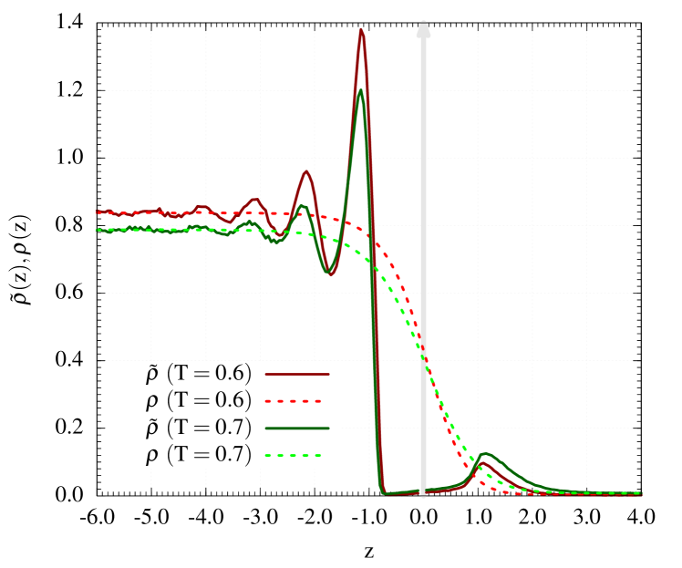
Figure 1: (Colour online). Intrinsic density profiles $\displaystyle\tilde{\rho}(z)$ (solid line) compared to mean density $\displaystyle\rho(z)$ (dashed line) for systems at $\displaystyle T=0.6$ (red colour) and $\displaystyle T=0.7$ (green colour), respectively. Surface atoms are represented by the delta function, represented as a grey arrow at $\displaystyle z=0$. The mean density profiles were centred at their corresponding Gibbs dividing surfaces $\displaystyle\left<\xi\right>$.

Fig. 1 depicts the intrinsic profiles at $\displaystyle T=0.6$ and $\displaystyle T=0.7$ respectively, obtained using the largest wavevector cutoff $\displaystyle k_{u}=2\pi$. Intrinsic quantities are plotted in a frame centred on the intrinsic surface, with the corresponding fixed grid quantities centred on the location of the appropriate Gibbs dividing surface. For convenience, these are both denoted as being at $\displaystyle z=0$ in all Figures. The removal of the blurring effect of thermal fluctuations results in the clear appearance of the molecular structure at the interface, given by the delta-function at $\displaystyle z=0$ representing the surface layer, followed by a strong oscillatory structure whose amplitude decays to zero at the bulk liquid density, and an adsorption peak at $\displaystyle z\approx 1.0$ in agreement with previous results (Chacón et al., 2009; Chacón and Tarazona, 2005).

The kinetic and configurational components of the intrinsic pressure profile (cf. Eq. (12)) at $\displaystyle T=0.6$ are depicted in Fig. 2. The dyadic terms $\displaystyle m_{i}\mathbf{v}_{i}\mathbf{v}_{i}$ in the kinetic component $\displaystyle\tilde{\mathbf{P}}^{k}$, being a single particle property, are as result directly proportional to the intrinsic density through the kinetic equation of state $\displaystyle\tilde{P}^{k}\left(z\right)=\tilde{\rho}\left(z\right)\,k_{B}T$, where $\displaystyle k_{B}$ is the Boltzmann’s constant. At constant temperature, these are all equal, emphasising the well known fact that, in the absence of temperature gradients, surface tension is a configurational property as attested by the configurational terms $\displaystyle\tilde{\mathbf{P}}^{c}$ (Kirkwood and Buff, 1949). On the liquid phase, away from the interface (viz. $\displaystyle\textstyle z\lesssim-4.0$), these are equivalent by a symmetry argument, i.e. the configurational pressure tensor is isotropic (the negative value reflects the cohesive energy of the LJ interactions).

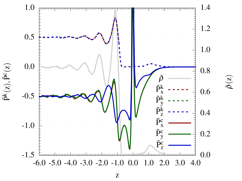
Figure 2: (Colour online). Kinetic and configurational components of the intrinsic pressure tensor, $\displaystyle\tilde{\mathbf{P}}^{k}\left(z\right)$ and $\displaystyle\tilde{\mathbf{P}}^{c}\left(z\right)$, at $\displaystyle T=0.6$. At constant temperature, $\displaystyle\tilde{P}^{k}_{x}$ (dashed red), $\displaystyle\tilde{P}^{k}_{y}$ (dashed green) and $\displaystyle\tilde{P}^{k}_{z}$ (dashed blue), are identical and proportional to the intrinsic density. Cylindrical symmetry about the normal axis gives identical configurational terms parallel to the interface, $\displaystyle\tilde{P}^{c}_{x}$ (red line) and $\displaystyle\tilde{P}^{c}_{y}$ (green line), within statistical uncertainty. The configurational pressure normal to the interface, $\displaystyle\tilde{P}^{c}_{c}$ (blue line), is significantly larger in the intermediate regions between the peaks the intrinsic density profile. The intrinsic density, $\displaystyle\tilde{\rho}\left(z\right)$ (grey line), is plotted on the secondary vertical axis.

In the layers closer to the interface, fluctuations in density break the symmetry of interactions. Fig. 3 illustrates this difference in more detail for $\displaystyle\tilde{P}_{N}=\tilde{P}_{z}$ and $\displaystyle\tilde{P}_{T}=(\tilde{P}_{x}+\tilde{P}_{y})/2$, at $\displaystyle T=0.6$ and $\displaystyle T=0.7$ respectively. The transverse pressure $\displaystyle\tilde{P}_{T}$ follows closely the oscillations in density, supporting the notion that, at the peaks in the intrinsic density, the larger number of neighbours interacting with an atom in the directions parallel to the interface results in a higher proportion of short ranged repulsive interactions contributing to the extra stress.

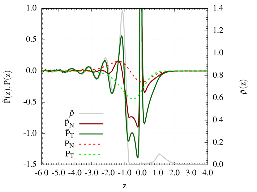
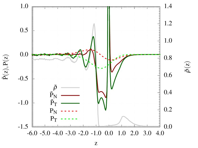
Figure 3: (Colour online). Top panel: components of the intrinsic pressure tensor tensor normal, $\displaystyle\tilde{P}_{N}=\tilde{P}_{z}$ (red colour), and transversal to the interface, $\displaystyle\tilde{P}_{T}=(\tilde{P}_{x}+\tilde{P}_{y})/2$ (green colour), at $\displaystyle T=0.6$. The mean profiles $\displaystyle P_{N}$ (dashed red line) and $\displaystyle P_{T}$ (dashed green line) are plotted for comparison. The intrinsic density, $\displaystyle\tilde{\rho}\left(z\right)$ (grey), is plotted on the secondary vertical axis. Bottom panel: intrinsic and average pressure profiles normal and transversal to the interface at $\displaystyle T=0.7$. The notation is the same as top panel.

On the other hand, in the normal direction, $\displaystyle\tilde{P}_{N}$ exhibits a more steady profile up until the region between the first two layers in the liquid phase. While being zero at the peak locations, reflecting mechanical equilibrium of the liquid layers (cf. Fig. 3, viz. $\displaystyle\textstyle z\approx-1\times 2^{1/6}$ and $\displaystyle\textstyle z\approx-2\times 2^{1/6}$), there is a clear positive excess normal pressure between these at $\displaystyle z\approx 1.5$. The physical argument behind this excess energy resides in the observation that an atom located at this position would experience the short range repulsive forces of the adjacent fluid layers. The resultant instability would force the atom to transit to one of the layers thus preserving the liquid structure next to the interface. We note that at larger distances from the interface, the mean normal pressure $\displaystyle P_{N}$ is equal in the liquid and vapour phase, as can be seen in Fig. 3. Over the surface the mean divergence of pressure will still be equal to zero, i.e. mechanical equilibrium must be satisfied as the surface is stationary.

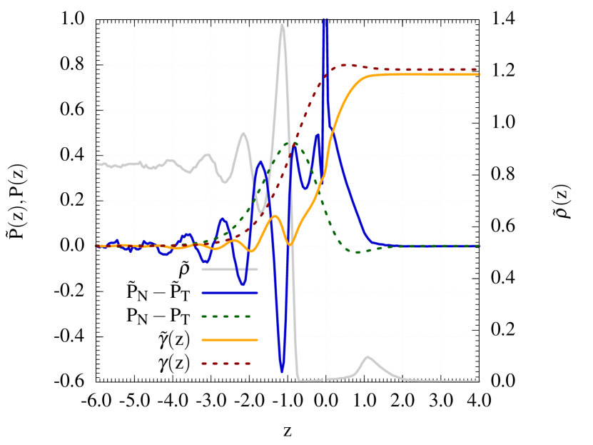
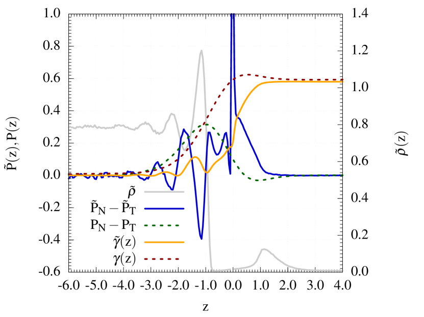
Figure 4: (Colour online). Top panel: comparison between excess intrinsic pressure, $\displaystyle\tilde{P}_{N}-\tilde{P}_{T}$ (blue colour), and its mean counterpart (green colour) at $\displaystyle T=0.6$. The bottom panel shows the results at $\displaystyle T=0.7$. The notation is the same as top panel.

Fig. 4 depicts the excess pressure of the fluid, defined by $\displaystyle\tilde{P}_{N}\left(z\right)-\tilde{P}_{T}\left(z\right)$, whose integral over the entire domain, $\displaystyle\textstyle\gamma\left(z\right)=\int_{-\infty}^{z}\,\mathrm{d}z^{\prime}\,\left(P_{N}\left(z^{\prime}\right)-P_{T}\left(z^{\prime}\right)\right)$, gives the Kirkwood-Buff (Kirkwood and Buff, 1951) definition of the surface tension (cf. Eq. (15) and Eq. (16)). At the highest molecular resolution, the intrinsic pressure tensor Eq. (12) allows us to ascertain the microscopic mechanism involved in giving rise to the interfacial energy.

We can observe that the surface tension has contributions from both the liquid and vapour facing sides of the (intrinsic) interface. Importantly, however, we note that the depletion region between the first layer of fluid at the surface layer is where the onset of the surface tension takes place. We are also able to see that the adsorption peak – approximately one fluid layer away from the surface – is vital to the contribution of the other half of the surface tension. Crucially, this is truly an adsorption peak rather than a density oscillation around the bulk vapour density (in contrast to the liquid facing side of the interface), due to the attraction of the vapour particles to the liquid (of course, as they are the same atoms). As the density increases and returns to the bulk vapour density, there is a net additive contribution to surface tension.

The physical picture is thus as follows: the surface tension, unlike the traditional mechanical picture – defined as the excess pressure acting across a surface of zero width between the liquid and vapour phases – arises instead across a boundary region spanning the three key layers involved in the intrinsic surface – the adsorbed layer at $\displaystyle z\approx 1.0$, the surface layer at $\displaystyle z=0$ and the first layer in the liquid phase at $\displaystyle z\approx-1.0$. This region is constructed by pairs of layers attracting each other in an interleaved manner, at a distance commensurate with the attractive tail of the Lennard-Jones potential – the adsorbed layer at $\displaystyle z\approx 1.0$ with the first liquid layer at $\displaystyle z\approx-1.0$ and surface layer at $\displaystyle z=0$ with the second liquid layer at $\displaystyle z\approx-2.0$ respectively.

The results shown in Fig. 4 demonstrate that the surface tension force has similar contributions on either side of the interface, an observation first given in (Sega, Fábián, and Jedlovszky, 2015), but shown here with unprecedented clarity using the intrinsic pressure derived in this work.

V Conclusion

We have proposed a generalisation of Irving and Kirkwood’s expression for the pressure tensor free from the smearing effect of thermal fluctuations of capillary waves. This is accomplished by letting the contour of integration become a dynamic quantity, unique to each pair of interacting particles, that reflects the instantaneous local curvature of the interface. Expressing hydrodynamic fields in control volume format, we are able to compute the intrinsic density profile that matches the profiles reported previously.

Applying the same technique to pressure allows the derivation of an intrinsic pressure tensor, which gives unprecedented insight into the liquid-vapour interface. More importantly, however, the notion of a mathematical surface of infinitesimal width, central to the mechanical definition of the surface tension, looses meaning at the microscopic level where the discrete nature of matter becomes apparent. Instead, we observe the emergence of the surface tension over a finite range of three atomic layers, acting exactly across the intrinsic surface.

The surface tension and other quantities of interest are derived from the continuity equations of hydrodynamics – expressed in a Lagrangian frame of reference relative to the intrinsic surface – and therefore are valid arbitrarily far from equilibrium. This makes the derived expressions particularly useful to the study of non equilibrium inhomogeneous systems – e.g., Marangoni flow, hydrodynamic instabilities and bubble nucleation, which are inherently non-local and unsteady. Of particular interest would also be extension of this study to systems in confinement including heterogeneous substrates and nanochannels (e.g. Refs Yatsyshin et al., 2017; Morciano et al., 2017).

essential in a range of important industrial processes where the surface tension plays a role, such as Marangoni flows, hydrodynamic instabilities and bubble nucleation, which are inherently non-equilibrium, non-local and unsteady.