The new $a_{1}(1420)$ state: structure, mass and width

Abstract

The structure, spectroscopic parameters and width of the resonance with quantum numbers $J^{PC}=1^{++}$ discovered by the COMPASS Collaboration and classified as the $a_{1}(1420)$ meson are examined in the context of QCD sum rule method. In the calculations the axial-vector meson $a_{1}(1420)$ is treated as a four-quark state with the diquark-antidiquark structure. The mass and current coupling of $a_{1}(1420)$ are evaluated using QCD two-point sum rule approach. Its observed decay mode $a_{1}(1420)\to f_{0}(980)\pi$, and kinematically allowed ones, namely $a_{1}\to K^{\ast\pm}K^{\mp}$, $a_{1}\to K^{\ast 0}\bar{K}^{0}$ and $a_{1}\to\bar{K}^{\ast 0}K^{0}$ channels are studied employing QCD sum rules on the light-cone. Our prediction for the mass of the $a_{1}(1420)$ state $m_{a_{1}}=1416_{-79}^{+81}\ \mathrm{MeV}$ is in excellent agreement with the experimental result. Width of this state $\Gamma=145.52\pm 20.79\mathrm{MeV}$ within theoretical and experimental errors is also in accord with the COMPASS data.

I Introduction

Classification of the light scalar and axial-vector meson multiplets is among of long-standing and ongoing problems of hadron spectroscopy Patrignani:2016xqp . The conventional theory of mesons that considers them as particles composed of a quark and antiquark $q\bar{q}$ meets with abundance of observed light states that should be included into this scheme. In fact, the family of axial-vector mesons contained till now five states with the spin-parities $J^{PC}=1^{++}$ Chen:2015iqa , recently enlarged due to discovery by COMPASS Collaboration of a new resonance $a_{1}(1420)$ with the same quantum numbers Adolph:2015pws . Some of these states including $a_{1}(1420)$ meson were listed in Ref. Patrignani:2016xqp , others wait detailed experimental explorations to confirm their status. It seems new theoretical models are required to explain all variety of available and forthcoming experimental information.

The COMPASS Collaboration analyzed the diffractive reaction $\pi^{-}+p\to\pi^{-}\pi^{-}\pi^{+}+p_{\mathrm{recoil}}$ and studied $J^{PC}=1^{++}$ states in order to find a possible partner of the isosinglet $f_{1}(1420)$ meson. In the $f_{0}(980)\pi$ final state the Collaboration observed a resonance $1^{++}$ and identified it as $a_{1}(1420)$ meson with the mass and width

$$m=1414^{+15}_{-13}\ \mathrm{MeV},\ \Gamma=153^{+8}_{-23}\ \mathrm{MeV}.$$ (1)

The discovery of the new light unflavored axial-vector state $a_{1}(1420)$ which presumably is isovector partner of $f_{1}(1420)$ meson, triggered theoretical investigations in the context of different models aiming to understand its quark-gluon structure and calculate its parameters . It is interesting that by classifying $a_{1}(1420)$ as an axial-vector meson the COMPASS Collaboration did not exclude its interpretation as an exotic state Adolph:2015pws . One of reasons pointed out there is observation of only $a_{1}(1420)\rightarrow f_{0}(980)\pi$ decay mode of the new meson $a_{1}(1420)$. The abundance of axial-vector mesons in the mass interval $1.2\div 2\ \mathrm{GeV}$, and difficulties in interpretation of $a_{1}(1420)$ as a radial excitation of the ground-state meson $a_{1}(1260)$ because of a small mass gap between them, also support attempts to interpret it as an exotic state.

The final particle of the decay $a_{1}(1420)\to f_{0}(980)\pi$, namely the $f_{0}(980)$ meson provides an additional information on possible structure of the $a_{1}(1420)$ meson. It is one of first mesons that was considered as candidate for a light four-quark state. Thus, already at early years of the quark-parton model it was supposed that the scalar meson $f_{0}(980)$ instead of traditional $\bar{q}q$ structure may have $\bar{q}^{2}q^{2}$ composition Jaffe:1976ig . Due to a substantial $s$-quark component it was treated also as the $K\bar{K}$ molecule Weinstein:1990gu . Lattice simulations and experimental exploration seem confirm assumptions on the exotic nature of $f_{0}(980)$ and some other hadrons Alford:2000mm ; Amsler:2004ps ; Bugg:2004xu ; Klempt:2007cp . Suggestions about a diquark-antidiquark structure of the light scalar mesons including $f_{0}(980)$ one were made on the basis of new theoretical analysis in Refs. Maiani:2004uc ; Hooft:2008we , as well.

Sum rules studies of the light scalar nonet led to controversial conclusions on their nature Latorre:1985uy ; Narison:1986vw ; Brito:2004tv ; Wang:2005cn ; Chen:2007xr ; Lee:2005hs ; Sugiyama:2007sg ; Kojo:2008hk ; Wang:2015uha . Thus, calculations carried out in some of these works confirmed the diquark-antidiquark structure of the light scalar particles Brito:2004tv ; Wang:2005cn ; Chen:2007xr , whereas in Ref. Lee:2005hs an evidence for a diquark component in the light scalar mesons was not found. Mixing of various diquark-antidiquarks with different flavor structures Chen:2007xr , superposition of diquark-antidiquark and $q\bar{q}$ constituents Sugiyama:2007sg ; Kojo:2008hk ; Wang:2015uha were examined to understand internal organization and explain experimental features of the light scalars.

It is seen that different theoretical models consider the $f_{0}(980)$ meson predominantly as a tetraquark state, or at least as a particle containing substantial four-quark component. This circumstance alongside with above arguments may give one a hint on possible exotic structure of the master particle $a_{1}(1420)$ itself. Really, soon after observation of the $a_{1}(1420)$ meson various scenarios that treated it as an exotic state appeared in literature. In Ref. Wang:2014bua the $a_{1}(1420)$ meson was realized as superposition of diquark-antidiquark and two-quark states. The mass of this compound, in accordance with conclusions of Ref. Wang:2014bua agrees with experimental data of the COMPASS Collaboration. The $a_{1}(1420)$ meson as a pure diquark-antidiquark state was explored in Ref. Chen:2015fwa , results of which are in accord with data, as well. It is worth noting that in both of these works QCD two-point sum rule method were used.

Another confirmation of the multi-quark nature of $a_{1}(1420)$ came from studies carried out in Ref. Gutsche:2017oro within the soft-wall AdS/QCD approach, where Schrodinger-type equation for the tetraquark wave function was derived and solved analytically. The prediction for the mass of the $J^{PC}=1^{++}$ tetraquark state obtained there agrees with data of Ref. Adolph:2015pws .

Alternative explanations of $a_{1}(1420)$ as manifestation of dynamical rescattering effects in $a_{1}(1260)$ meson’s decays are presented in the literature by a number of papers Ketzer:2015tqa ; Liu:2015taa ; Aceti:2016yeb ; Basdevant:2015wma ; Wang:2015cis . In fact, the resonance in the $f_{0}(980)\pi$ final state was explained in Ref. Ketzer:2015tqa as a triangle singularity appearing in the relevant decay mode of the $a_{1}(1260)$ meson. In accordance with the proposed scheme this decay proceeds through three stages: at the fist step $a_{1}(1260)$ decays to a pair of $K^{\ast}\bar{K}$-mesons, at the second stage $K^{\ast}$ meson decays to $K$ and $\pi$. At the final phase $K$ and $\bar{K}$ combine to create the $f_{0}(980)$ meson. Analysis of these processes and calculation of corresponding triangle diagram using the effective Lagrangian approach reveals a singularity that may be interpreted as the resonance seen by the COMPASS Collaboration. The same ideas were shared by Ref. Liu:2015taa , where manifestation of the anomalous triangle singularity were analyzed in various processes, including $a_{1}(1260)\rightarrow f_{0}(980)\pi$ decay.

Recently, problems of the two-body strong decays of $a_{1}(1420)$ were addressed in Ref. Gutsche:2017twh . In this work partial decay channels of $a_{1}(1420)$ were investigated in the framework of the covariant confined quark model by treating $a_{1}(1420)$ as a tetraquark with both diquark-antidiquark and molecular structures. When considering the decay $a_{1}(1420)\to f_{0}(980)\pi$ the final-state meson $f_{0}(980)$ was also chosen as the tetraquark state with molecular or diquark composition. The partial decay widths, and the full width of the $a_{1}(1420)$ state calculated in this paper allowed authors to conclude that it is a four-quark state, and a molecular configuration for $a_{1}(1420)$ is preferable than the diquark-antidiquark structure.

As is seen, theoretical interpretations of the axial-vector state $a_{1}(1420)$ can be divided into two almost equal classes: in some of papers it is treated as a four-quark system with different structures, in others - considered as dynamical rescattering effect seen in the decay $a_{1}(1260)\rightarrow f_{0}(980)\pi$.

In the present work we are going to test $a_{1}(1420)$ as an axial-vector diquark-antidiquark state, and at the first phase of our investigations, calculate its mass and current coupling. To this end, we will make use of QCD two-point sum rule approach by taking into account various vacuum condensates up to dimension twelve Shifman1 ; Shifman2 . We will afterwards investigate two-body strong decay channels of the $a_{1}(1420)$ meson and compute strong couplings $g_{[\ldots]}$ corresponding to the vertices $a_{1}f_{0}\pi$, $a_{1}K^{\ast\pm}K^{\mp},a_{1}K^{\ast 0}\bar{K}^{0}$ and $a_{1}\bar{K}^{\ast 0}K^{0}$. These couplings are crucial for calculation of the partial width of the decay modes $a_{1}\rightarrow f_{0}(980)\pi,\ a_{1}\rightarrow K^{\ast\pm}K^{\mp},\ K^{\ast 0}\bar{K}^{0}$ and $\ \bar{K}^{\ast 0}K^{0}$.

The strong couplings will be computed in the framework of the QCD light-cone sum rule (LCSR) approach Balitsky:1989ry ; Belyaev:1994zk , which is one of the most reliable and universal nonperturbative methods to explore hadrons’ spectroscopic parameters and their decay modes. We will study the decay $a_{1}\rightarrow f_{0}(980)\pi$ by treating the $f_{0}(980)$ meson as the diquark-antidiquark state and evaluate the strong coupling $g_{a_{1}f_{0}\pi}$ in the context of the full LCSR method. The reason is that after contracting quark fields from interpolating currents for $a_{1}(1420)$ and $f_{0}(980)$ a relevant correlation function depends on distribution amplitudes (DAs) of the pion. In the case of vertices composed of the $a_{1}(1420)$ state and two conventional mesons one has to apply LCSR method in conjunction with technical tools of the soft-meson approximation. In the soft approximation a correlation function instead of DAs depends on local matrix elements of a final light meson, and as a result, to preserve four-momentum conservation at a vertex one should set its momentum equal to zero Agaev:2016dev . Additionally, to remove unsuppressed terms from the phenomenological side of sum rules one has to perform operations explained in Refs. Belyaev:1994zk ; Ioffe:1983ju . The LCSR method and soft approximation were adapted to study vertices involving a tetraquark and conventional mesons in our work Agaev:2016dev , and was later applied to investigate decays of various tetraquarks Agaev:2016dsg ; Agaev:2017uky ; Agaev:2017foq ; Agaev:2017tzv ; Agaev:2017oay .

The present work is structured in the following manner: In Sec. II we calculate the mass and current coupling of the $a_{1}(1420)$ meson by treating it as a diquark-antidiquark state. These parameters will be used later to calculate widths of the $a_{1}(1420)$ meson’s strong decay channels. In the next Section we examine the vertex $a_{1}(1420)f_{0}(980)\pi\equiv a_{1}f_{0}\pi$, and calculate the strong coupling $g_{a_{1}f_{0}\pi}$ and width of the $P$-wave decay $a_{1}(1420)\rightarrow f_{0}(980)\pi$. Section IV is devoted to exploration of the $S$-wave processes $a_{1}\rightarrow K^{\ast\pm}K^{\mp},\ K^{\ast 0}\bar{K}^{0}$ and $\ \bar{K}^{\ast 0}K^{0}$, where we present sum rule predictions for relevant strong couplings and partial decay widths. Here we also determine full width of the $a_{1}(1420)$ state. Section V contains our concluding notes. The light quark propagators and lengthy analytical expression for the correlation function $\Pi_{\mathrm{V}}(M^{2},s_{0})$ are written down in Appendix.

II Mass and current coupling of $a_{1}(1420)$

The $a_{1}(1420)$ state is a neutral isovector meson with $I^{G}J^{PC}=1^{-}1^{++}$. In the diquark picture its quark content has the form $([us][\bar{u}\bar{s}]-[ds][\bar{d}\bar{s}])/\sqrt{2}$, whereas the isoscalar partner of $a_{1}(1420)$, namely $f_{1}(1420)$ will have the composition $([us][\bar{u}\bar{s}]+[ds][\bar{d}\bar{s}])/\sqrt{2}$. In the chiral limit adopted in present paper the particles $a_{1}(1420)$ and $f_{1}(1420)$ have equal masses (see, Ref. Chen:2015fwa ).

The next problem is connected with the flavor structure of the interpolating current. It may have symmetric, antisymmetric or mixed-symmetric type flavor structures. In the present work for the $a_{1}(1420)$ meson we choose an interpolating current that belongs to a class of currents with the mixed-type flavor symmetry (detailed discussion of these questions was presented in Ref. Chen:2015fwa )

$$J_{\mu}(x)=\frac{1}{\sqrt{2}}[J_{\mu}^{u}(x)-J_{\mu}^{d}(x)],$$ (2)

where

$$J_{\mu}^{q}(x)=q_{a}^{T}(x)C\gamma_{5}s_{b}(x)\left[\overline{q}_{a}(x)\gamma_{\mu}C\overline{s}_{b}^{T}(x)\right.$$

$$\left.-\overline{q}_{b}(x)\gamma_{\mu}C\overline{s}_{a}^{T}(x)\right]+q_{a}^{T}(x)C\gamma_{\mu}s_{b}(x)$$

$$\times\left[\overline{q}_{a}(x)\gamma_{5}C\overline{s}_{b}^{T}(x)-\overline{q}_{b}(x)\gamma_{5}C\overline{s}_{a}^{T}(x)\right].$$ (3)

In Eq. (3) $q$ is one of the light $u,\ d$ quarks, $a,b$ are color indices and $C$ is the charge conjugation operator.

Having fixed the current $J_{\mu}(x)$ we start to calculate the correlation function which enables us to extract the mass $m_{a_{1}}$ and coupling $f_{a_{1}}$ of the $a_{1}(1420)$ state. The correlation function necessary for our purposes is given by the expression:

$$\Pi_{\mu\nu}(p)=i\int d^{4}xe^{ip\cdot x}\langle 0|\mathcal{T}\{J_{\mu}(x)J_{\nu}^{\dagger}(0)\}|0\rangle.$$ (4)

In accordance with usual prescriptions of QCD sum rules one has to express $\Pi_{\mu\nu}(p)$ in terms of physical parameters of the axial-vector particle(s). We use here “a ground-state + continuum” approximation by supposing that the current $J_{\mu}(x)$ couples to only $a_{1}(1420)$ meson. In this framework $\Pi_{\mu\nu}^{\mathrm{Phys}}(p)$ takes the following form

$$\Pi_{\mu\nu}^{\mathrm{Phys}}(p)=\frac{m_{a_{1}}^{2}f_{a_{1}}^{2}}{m_{a_{1}}^{2}-p^{2}}\left(-g_{\mu\nu}+\frac{p_{\mu}p_{\nu}}{p^{2}}\right)+\ldots$$ (5)

where the dots indicate contributions of the higher resonances and continuum states. To derive $\Pi_{\mu\nu}^{\mathrm{Phys}}(p)$ we use the matrix element of the $a_{1}(1420)$ meson

$$\langle 0|J_{\mu}|a_{1}(p)\rangle=f_{a_{1}}m_{a_{1}}\epsilon_{\mu},$$ (6)

where $m_{a_{1}},$ $f_{a_{1}}$and $\epsilon_{\mu}$ are the mass, the coupling and the polarization vector of the $a_{1}(1420)$ state, respectively.

The next phase of studies implies calculation of the correlation function $\Pi_{\mu\nu}(p)$ using the quark-gluon degrees of freedom. This means that one has to substitute the interpolating current defined by Eqs. (2) and (3) into Eq. (4) and contract quarks fields that generate light quark propagators, explicit expression of which is moved to Appendix. The general form of the correlation function then is:

$$\Pi_{\mu\nu}^{\mathrm{OPE}}(p)=\Pi_{\mathrm{V}}(p^{2})\left(-g_{\mu\nu}+\frac{p_{\mu}p_{\nu}}{p^{2}}\right)+\Pi_{\mathrm{S}}(p^{2})\frac{p_{\mu}p_{\nu}}{p^{2}},$$ (7)

where $\Pi_{\mathrm{V}}(p^{2})$ and $\Pi_{\mathrm{S}}(p^{2})$ are invariant amplitudes receiving a contribution only from an axial-vector and scalar particles, respectively. Because we are interested in parameters of the axial-vector state $a_{1}(1420)$ we choose the Lorentz structure $g_{\mu\nu}$ and corresponding function $\Pi_{\mathrm{V}}(p^{2})$ to derive desired sum rules. To this end, we apply the Borel transformation to $\Pi_{\mu\nu}^{\mathrm{Phys}}(p)$ and $\Pi_{\mu\nu}^{\mathrm{OPE}}(p)$, pick out $\mathcal{B}\Pi_{\mathrm{V}}(p^{2})=\Pi_{\mathrm{V}}(M^{2})$ and equate it to relevant piece from the phenomenological side of the sum rule

$$m_{a_{1}}^{2}f_{a_{1}}^{2}e^{-m_{a_{1}}^{2}/M^{2}}+\ldots=\Pi_{\mathrm{V}}(M^{2}).$$ (8)

In terms of the spectral density $\rho(s)$ the Borel transformation of $\Pi_{\mathrm{V}}(p^{2})$ takes very simple form and reads

$$\Pi_{\mathrm{V}}(M^{2})=\int_{4m_{s}^{2}}^{\infty}ds\rho(s)e^{-s/M^{2}}.$$ (9)

In order to derive sum rules one has to subtract contributions of the higher resonances and continuum states. This can be achieved by invoking of assumption about the quark-hadron duality and replacing

$$\int_{4m_{s}^{2}}^{\infty}ds\rho(s)e^{-s/M^{2}}\rightarrow\int_{4m_{s}^{2}}^{s_{0}}ds\rho(s)e^{-s/M^{2}},$$ (10)

where $s_{0}$ is the continuum threshold parameter: It separates ground-state and continuum contributions from each other. Alternatively, Borel transform of $\Pi_{\mathrm{V}}(p^{2})$ may be calculated directly from its expression avoiding intermediate steps. Then continuum subtraction is fulfilled in terms that are $\sim(M^{2})^{n},\ n=1,\ 2,\dots$ Belyaev:1994zk .

In the present paper we calculate $\Pi_{\mathrm{V}}(M^{2})$ by taking into account various condensates up to dimension twelve. Contributions of terms up to dimension eight are obtained utilizing relevant spectral densities, remaining terms are found by means of direct Borel transformation. Sum rules for the mass and coupling of the $a_{1}(1420)$ state can be obtained from subtracted version of Eq. (8) by means of standard operations. After continuum subtraction $\Pi_{\mathrm{V}}(M^{2},\ s_{0})$ acquires a dependence also on the continuum threshold parameter $s_{0}$. The final result for $\Pi_{\mathrm{V}}(M^{2},s_{0})$ is written down in Appendix.

The quark propagators, and as a result sum rules for the mass and coupling depend on numerous parameters, values of which should be specified to perform numerical computations. Below we list the mass of the $s$-quark, and vacuum expectation values of the quark, gluon and mixed local operators

$$m_{s}=128_{-6}^{+10}~{}\mathrm{MeV}$$

$$\langle\bar{q}q\rangle=-(0.24\pm 0.01)^{3}\ \mathrm{GeV}^{3},\ \langle\bar{s}s\rangle=0.8\ \langle\bar{q}q\rangle,$$

$$m_{0}^{2}=(0.8\pm 0.1)\ \mathrm{GeV}^{2},\ \langle\overline{q}g_{s}\sigma Gq\rangle=m_{0}^{2}\langle\overline{q}q\rangle,$$

$$\langle\overline{s}g_{s}\sigma Gs\rangle=m_{0}^{2}\langle\bar{s}s\rangle,$$

$$\langle\frac{\alpha_{s}G^{2}}{\pi}\rangle=(0.012\pm 0.004)\,\mathrm{GeV}^{4},$$

$$\langle g_{s}^{3}G^{3}\rangle=(0.57\pm 0.29)\ \mathrm{GeV}^{6}.$$ (11)

It is useful to note that for $m_{s}$ we use its value rescaled to $\mu=1\ \mathrm{GeV}$ Patrignani:2016xqp .

Sum rules depend also on auxiliary parameters $M^{2}$ and $s_{0}$ the choice of which has to satisfy standard restrictions. Performed analyses allow us to fix the working regions for $M^{2}$ and $s_{0}$:

$$M^{2}\in[1.4,\ 1.8]\ \mathrm{GeV}^{2},\ s_{0}\in[2.4,\ 3.1]\ \mathrm{GeV}^{2}.$$ (12)

In Figs. 1 and 2 we depict the sum rules results for the mass and current coupling of the $a_{1}(1420)$ state as functions of the Borel and continuum threshold parameters. As is seen, prediction for the mass is rather stable against varying of both $M^{2}$ and $s_{0}.$ The dependence of $f_{a_{1}}$ on the Borel parameter at fixed $s_{0}$ is very weak, whereas its variations with $s_{0}$ are noticeable and generate substantial part of theoretical errors.

For $m_{a_{1}}$ and $f_{a_{1}}$ we find:

$$m_{a_{1}}=1416_{-79}^{+81}\ \ \mathrm{MeV},\ f_{a_{1}}=(1.68_{-0.26}^{+0.25}\ )\cdot 10^{-3}\ \ \mathrm{GeV}^{4}.$$ (13)

Our result for the mass of the $a_{1}(1420)$ state is in excellent agreement with data of the COMPASS Collaboration. It agrees also with the mass of the $a_{1}(1420)$ meson obtained previously in the diquark-antidiquark picture in Ref. Chen:2015fwa

$$m_{a_{1}}=(1440\pm 80)\ \ \mathrm{MeV},\ f_{a_{1}}=(1.32\pm 0.35\ )\cdot 10^{-3}\ \ \mathrm{GeV}^{4}.$$ (14)

Within the theoretical errors the coupling $f_{a_{1}}$ is compatible with the result of Ref. Chen:2015fwa : there is a large overlap region between two predictions. It is worth noting that we have rescaled the coupling $\widetilde{f}_{a_{1}}\equiv f_{a_{1}}m_{a_{1}}=$ $(1.9\pm 0.5\ )\cdot 10^{-3}\ \ \mathrm{GeV}^{5}$ in accordance with our definition Eq. (6) using for this purpose $m_{a_{1}}$ from Eq. (14). Numerical difference between two sets of parameters stems from some subleading terms in the corresponding spectral densities, which however do not affect considerably the final results, as is seen from Eqs. (13) and (14).

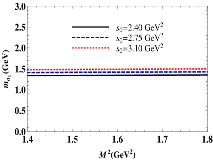
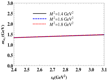
Figure 1: The mass of the $a_{1}$ state as a function of the Borel parameter $M^{2}$ at fixed $s_{0}$ (left panel), and as a function of the continuum threshold $s_{0}$ at fixed $M^{2}$ (right panel).

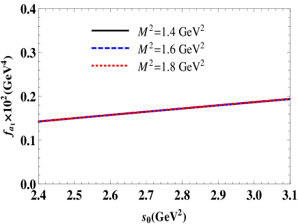
Figure 2: The current coupling $f_{a_{1}}$ of the $a_{1}$ state as a function of $M^{2}$ at fixed $s_{0}$ (left panel), and of $s_{0}$ at fixed $M^{2}$ (right panel).

III The decay channel $a_{1}(1420)\to f_{0}(980)\pi^{0}$

The decay $a_{1}(1420)\rightarrow f_{0}(980)\pi^{0}$ which was observed by the COMPASS Collaboration and led to discovery of the axial-vector state $a_{1}(1420)$ is a $P$-wave transition and consequently is not its dominant decay channel. Nevertheless, it should be properly analyzed because still remains solely observed decay of the $a_{1}(1420)$ state . In the context of the QCD light-cone sum rule method this process can be investigated starting from the correlation function

$$\Pi_{\mu}(p,q)=i\int d^{4}xe^{ip\cdot x}\langle\pi(q)|\mathcal{T}\{J^{f}(x)J_{\mu}^{\dagger}(0)\}|0\rangle,$$ (15)

where $J_{\mu}(0)$ is the interpolating current of $a_{1}(1420)$ which we treat in this work as the axial-vector diquark-antidiquark state, and $J^{f}(x)$ is the interpolating current of the scalar $f_{0}(980)$. In the light of above discussions it is clear that there are various models of $f_{0}(980)$ in the literature. In the present study we consider $f_{0}(980)$ as the scalar diquark-antidiquark state and choose the current $J^{f}(x)$ to interpolate it in the following form

$$J^{f}(x)=\frac{\epsilon^{dab}\epsilon^{dce}}{\sqrt{2}}\left\{\left[u_{a}^{T}(x)C\gamma_{5}s_{b}(x)\right]\left[\overline{u}_{c}(x)\gamma_{5}C\overline{s}_{e}^{T}(x)\right]\right.$$

$$\left.+\left[d_{a}^{T}(x)C\gamma_{5}s_{b}(x)\right]\left[\overline{d}_{c}(x)\gamma_{5}C\overline{s}_{e}^{T}(x)\right]\right\}.$$ (16)

After adopting the currents we analyze the vertex $a_{1}f_{0}\pi$ which is composed of two tetraquarks and a conventional meson, and in this aspect differs from ones containing a tetraquark and two ordinary mesons. In order to derive the sum rule for the strong coupling $g_{a_{1}f_{0}\pi}$ we carry out well-known standard operations. At the first stage we express the correlation function in terms of physical parameters of the involved particles and get

$$\Pi_{\mu}^{\mathrm{Phys}}(p,q)=\frac{\langle 0|J^{f}|f_{0}(p)\rangle}{p^{2}-m_{f_{0}}^{2}}\langle f_{0}\left(p\right)\pi(q)|a_{1}(p^{\prime})\rangle$$

$$\times\frac{\langle a_{1}(p^{\prime})|J_{\mu}^{\dagger}|0\rangle}{p^{\prime 2}-m_{a_{1}}^{2}}+...,$$ (17)

where the dots indicate contributions due to higher resonances and continuum states. The physical representation $\Pi_{\mu}^{\mathrm{Phys}}(p,q)$ of the correlator can be simplified by means of the matrix element given by Eq. (6), a new one defined as

$$\langle 0|J^{f}|f_{0}\left(p\right)\rangle=f_{f_{0}}m_{f_{0}},$$ (18)

as well as by introducing the strong coupling $g_{a_{1}f_{0}\pi}$ to specify the vertex

$$\langle f_{0}\left(p\right)\pi(q)|a_{1}(p^{\prime})\rangle=g_{a_{1}f_{0}\pi}p\cdot\varepsilon^{\prime\ast}.$$ (19)

Here $p^{\prime},\ p$ and $q$ are four-momenta of $a_{1}(1420),~{}f_{0}(980)$ and $\pi$, respectively. In Eq. (19) $\varepsilon^{\prime}$ is the polarization vector of the $a_{1}(1420)$ state. The two-variable Borel transformations applied to $\Pi_{\mu}^{\mathrm{Phys}}(p,q)$ yield

$$\mathcal{B}\Pi_{\mu}^{\mathrm{Phys}}(p,q)=g_{a_{1}f_{0}\pi}m_{f_{0}}m_{a_{1}}f_{f_{0}}f_{a_{1}}e^{-m_{f_{0}}^{2}/M_{1}^{2}-m_{a_{1}}^{2}/M_{2}^{2}}$$

$$\times\left[\frac{1}{2}\left(-1+\frac{m_{f_{0}}^{2}}{m_{a_{1}}^{2}}\right)p_{\mu}+\frac{1}{2}\left(1+\frac{m_{f_{0}}^{2}}{m_{a_{1}}^{2}}\right)q_{\mu}\right],$$ (20)

where $M_{1}^{2}$ and $M_{2}^{2}$ are the Borel parameters which correspond to $p^{2}$ and $p^{\prime 2}$, respectively. The $\Pi_{\mu}^{\mathrm{Phys}}(p,q)$ and its Borel transformed form contain two structures $\sim p_{\mu}$ and $\sim q_{\mu}$. In investigations we employ the invariant amplitude that correspond to the structure $\sim p_{\mu}$

$$\Pi^{\mathrm{Phys}}\left(M_{1}^{2},\ M_{2}^{2}\right)=g_{a_{1}f_{0}\pi}m_{f_{0}}m_{a_{1}}f_{f_{0}}f_{a_{1}}$$

$$\times\frac{1}{2}e^{-m_{f_{0}}^{2}/M_{1}^{2}-m_{a_{1}}^{2}/M_{2}^{2}}\left(-1+\frac{m_{f_{0}}^{2}}{m_{a_{1}}^{2}}\right).$$ (21)

In order to derive the sum rule we need to calculate its second component, which means that the correlation function $\Pi_{\mu}(p,q)$ has to be found in terms of quark propagators and distribution amplitudes of the pion. After substituting the currents into Eq. (15) and contracting quark fields we get

$$\Pi_{\mu}^{\mathrm{OPE}}(p,q)=i\int d^{4}x\epsilon\widetilde{\epsilon}\epsilon^{\prime}\widetilde{\epsilon}^{\prime}e^{ipx}\left\{\mathrm{Tr}\left[\gamma_{\mu}\widetilde{S}_{u}^{a^{\prime}a}(x){}\gamma_{5}\widetilde{S}_{s}^{b^{\prime}b}(x){}\right]\left[\gamma_{5}\widetilde{S}_{s}^{ee^{\prime}}(-x)\gamma_{5}{}\right]_{\alpha\beta}\langle\pi(q)|\overline{u}_{\alpha}^{c^{\prime}}(x)u_{\beta}^{c}(0)|0\rangle\right.$$

$$-\mathrm{Tr}\left[\gamma_{5}\widetilde{S}_{s}^{ee^{\prime}}(-x){}\gamma_{5}\widetilde{S}_{u}^{cc^{\prime}}(-x){}\right]\left[\gamma_{\mu}\widetilde{S}_{s}^{b^{\prime}b}(x)\gamma_{5}{}\right]_{\alpha\beta}\langle\pi(q)|\overline{u}_{\alpha}^{a}(x)u_{\beta}^{a^{\prime}}(0)|0\rangle+\mathrm{Tr}\left[\gamma_{5}\widetilde{S}_{u}^{a^{\prime}a}(x){}\gamma_{5}\widetilde{S}_{s}^{b^{\prime}b}(x)\right]$$

$$\times\left[\gamma_{5}\widetilde{S}_{s}^{ee^{\prime}}(-x)\gamma_{\mu}\right]_{\alpha\beta}\langle\pi(q)|\overline{u}_{\alpha}^{c^{\prime}}(x)u_{\beta}^{c}(0)|0\rangle+\mathrm{Tr}\left[\gamma_{5}\widetilde{S}_{s}^{ee^{\prime}}(-x)\gamma_{\mu}\widetilde{S}_{u}^{cc^{\prime}}(-x){}\right]\left[\gamma_{5}\widetilde{S}_{s}^{b^{\prime}b}(x)\gamma_{5}{}\right]_{\alpha\beta}\langle\pi(q)|\overline{u}_{\alpha}^{a}(x)u_{\beta}^{a^{\prime}}(0)|0\rangle,$$

where for brevity we use $\epsilon\widetilde{\epsilon}\epsilon^{\prime}\widetilde{\epsilon}^{\prime}=\epsilon^{dab}\epsilon^{dce}\epsilon^{d^{\prime}a^{\prime}b^{\prime}}\epsilon^{d^{\prime}c^{\prime}e^{\prime}}$.

In this expression $S_{u}(x)$ and $S_{s}(x)$ are the light $u$ and $s$ quarks light-cone propagators (see, Appendix). Let us emphasize that Eq. (LABEL:eq:CorrF4) is a whole expression for the correlation function, which encompasses terms appearing due to both $u$ and $d$ components of the interpolating currents $J_{\mu}(x)$ and $J^{f}(x)$. Because we work in the chiral limit this form of $\Pi_{\mu}^{\mathrm{OPE}}(p,q)$ is convenient for further analysis and calculations.

The function $\Pi_{\mu}^{\mathrm{OPE}}(p,q)$ apart from propagators contains also non-local quark operators sandwiched between the vacuum and pion states. These operators can be expanded over the full set of Dirac matrices $\Gamma^{j}$

$$\overline{u}_{\alpha}^{a}(x)u_{\beta}^{b}(0)\rightarrow\frac{1}{4}\Gamma_{\beta\alpha}^{j}\left[\overline{u}^{a}(x)\Gamma^{j}u^{b}(0)\right],$$ (23)

where $\Gamma^{j}$

$$\Gamma^{j}=\mathbf{1,\ }\gamma_{5},\ \gamma_{\mu},\ i\gamma_{5}\gamma_{\mu},\ \sigma_{\mu\nu}/\sqrt{2}.$$ (24)

Using the projector onto a color -singlet state $\delta^{ab}/3$ one finds

$$\overline{u}_{\alpha}^{a}(x)u_{\beta}^{b}(0)\rightarrow\frac{\delta^{ab}}{12}\Gamma_{\beta\alpha}^{j}\left[\overline{u}(x)\Gamma^{j}u(0)\right].$$ (25)

The matrix elements of operators $\overline{u}(x)\Gamma^{j}u(0)$ can be expanded over $x^{2}$ and expressed by means of the pion’s two-particle DAs of different twist Braun:1989iv ; Ball:1998je ; Ball:2006wn . For example, in the case of $\Gamma=\ i\gamma_{\mu}\gamma_{5}$ and $\gamma_{5}$ one obtains

$$\sqrt{2}\langle\pi^{0}(q)|\overline{u}(x)i\gamma_{\mu}\gamma_{5}u(0)|0\rangle$$ (26)

$$= f_{\pi}q_{\mu}\int_{0}^{1}due^{i\overline{u}qx}\left[\phi_{\pi}(u)+\frac{m_{\pi}^{2}x^{2}}{16}\mathbb{A}_{4}(u)\right]$$

$$+\frac{f_{\pi}m_{\pi}^{2}}{2}\frac{x_{\mu}}{qx}\int_{0}^{1}due^{i\overline{u}qx}\mathbb{B}_{4}(u),$$

and

$$\sqrt{2}\langle\pi^{0}(q)|\overline{u}(x)i\gamma_{5}u(0)|0\rangle=\frac{f_{\pi}m_{\pi}^{2}}{m_{u}+m_{d}}$$

$$\times\int_{0}^{1}due^{iuqx}\phi_{3;\pi}^{p}(u).$$ (27)

In Eq. (26) $\phi_{\pi}(u)$ is the leading twist (twist-2) distribution amplitude of the pion, whereas $\mathbb{A}_{4}(u)$ and $\mathbb{B}_{4}(u)$ are higher-twist functions that can be expressed using the pion two-particle twist-4 DAs. One of two-particle twist-3 distributions $\phi_{3;\pi}^{p}(u)$ determines the matrix element given by Eq. (27).  Another two-particle twist-3 DA $\phi_{3;\pi}^{\sigma}(u)$ corresponds to matix element with $\sigma_{\mu\nu}$ insertion. The non-local operators that appear due to a gluon field strength tensor $G_{\mu\nu}(ux)$ included into $\overline{u}(x)\Gamma^{j}u(0)$ generate the pion’s three-particle distributions. Their definitions and further details were presented in Ref. Braun:1989iv ; Ball:1998je ; Ball:2006wn .

The explicit expression of correlation function in terms of numerous DAs of the pion is rather cumbersome, therefore we do not provide it here. The $\Pi_{\mu}^{\mathrm{OPE}}(p,q)$ contains two Lorentz structures $\sim p_{\mu}$ and $\sim q_{\mu}$. We employ the invariant amplitude $\sim p_{\mu}$ to match it with corresponding function from $\Pi_{\mu}^{\mathrm{Phys}}(p,q)$. The Borel transform of the invariant amplitude under discussion, which we denote in what follows as $\Pi^{\mathrm{OPE}}\left(M_{1}^{2},\ M_{2}^{2}\right)$, can be calculated along a line explained in Ref. Belyaev:1994zk . At the next phase one must subtract contribution of higher resonances and continuum states. This procedure becomes easier when two Borel parameters are equal to each other $M_{1}^{2}=M_{2}^{2}$. In our case we suggest that a choice $M_{1}^{2}=M_{2}^{2}$ does not generate large uncertainties in sum rules and introduce $M^{2}$ through

$$\frac{1}{M^{2}}=\frac{1}{M_{1}^{2}}+\frac{1}{M_{2}^{2}},$$ (28)

which considerably simplifies studies. Continuum subtraction is fulfilled in accordance with methods described in Ref. Belyaev:1994zk . Some formulas used in this process can be found in Appendix B of Ref. Agaev:2016srl .

Then sum rule for the strong coupling $g_{a_{1}f_{0}\pi}$ reads

$$g_{a_{1}f_{0}\pi}=\frac{2m_{a_{1}}^{2}}{m_{f_{0}}^{2}-m_{a_{1}}^{2}}\frac{e^{(m_{f_{0}}^{2}+m_{a_{1}}^{2})/2M^{2}}}{m_{f_{0}}m_{a_{1}}f_{f_{0}}f_{a_{1}}}\Pi^{\mathrm{OPE}}\left(M^{2},\ s_{0}\right).$$ (29)

The partial width of decay $a_{1}(1420)\rightarrow f_{0}(980)\pi^{0}$ is given by the formula

$$\Gamma(a_{1}\rightarrow f_{0}\pi^{0})=g_{a_{1}f_{0}\pi}^{2}\frac{|\overrightarrow{p}|^{3}}{24\pi m_{a_{1}}^{2}},$$ (30)

where

$$|\overrightarrow{p}| = \frac{1}{2m_{a_{1}}}\left(m_{a_{1}}^{4}+m_{f_{0}}^{4}+m_{\pi}^{4}-2m_{f_{0}}^{2}m_{a_{1}}^{2}\right.$$ (31)

$$\left.-2m_{\pi}^{2}m_{a_{1}}^{2}-2m_{f_{0}}^{2}m_{\pi}^{2}\right)^{1/2}.$$

Important nonperturbative information in $\Pi^{\mathrm{OPE}}\left(M^{2},\ s_{0}\right)$ is encoded by the pion’s distribution amplitudes. A substantial part of $\Pi^{\mathrm{OPE}}\left(M^{2},\ s_{0}\right)$ forms due to two-particle DAs including $\phi_{\pi}(u)$ one, at the middle point $u_{0}=1/2$. The leading twist DA $\phi_{\pi}(u)$ through equations of motion affects other DAs of the pion. As a result, it contributes to $\Pi^{\mathrm{OPE}}\left(M^{2},\ s_{0}\right)$ not only directly, but also through higher-twist DAs of the pion, and deserves a detailed consideration.

The DA $\phi_{\pi}(u)$ has a following expansion over the Gegenbauer polynomials $C_{2n}^{3/2}(\varsigma)$

$$\phi_{\pi}(u,\mu^{2})=6u\overline{u}\left[1+\sum_{n=1,2,3\ldots}a_{2n}(\mu^{2})C_{2n}^{3/2}(u-\overline{u})\right],$$ (32)

where $\overline{u}=1-u$. In general, due to coefficients $a_{2n}(\mu^{2})$ it depends on a scale $\mu$, as well. Values of the Gegenbauer moments $a_{2n}(\mu^{2})$ at some normalization point $\mu=\mu_{0}$ have to be either extracted from phenomenological analysis or evaluated by employing, for example, lattice simulations.

In the present work we use two models for $\phi_{\pi}(u,\mu^{2}=1\ \mathrm{GeV}^{2}\ )$ . First of them was extracted in Ref. Agaev:2010aq ; Agaev:2012tm from LCSR analysis of the electromagnetic transition form factor of the pion. This DA is determined by the Gegenbauer moments

$$a_{2}=0.1,\ a_{4}=0.1,\ a_{6}=0.1,\ a_{8}=0.034,$$ (33)

and at the middle point equals to $\phi_{\pi}(1/2)\simeq 1.354$. This value is not far from $\phi_{\mathrm{asy}}(1/2)=3/2$, where $\phi_{\mathrm{asy}}(u)=6u\overline{u}$ is the asymptotic DA. We also employ the second model for $\phi_{\pi}(u)$ obtained in Ref. Braun:2015axa from lattice simulations. It contains only one non-asymptotic term

$$\phi_{\pi}(u,\mu^{2})=6u\overline{u}\left[1+a_{2}(\mu^{2})C_{2}^{3/2}(u-\overline{u})\right],$$ (34)

the second Gegenbauer moment $a_{2}(\mu^{2})$ of which at $\mu=2\ \mathrm{GeV}$ was estimated as $a_{2}=0.1364\pm 0.021$. It evolves to

$$a_{2}(1\ \mathrm{GeV}^{2})=0.1836\pm 0.0283,$$ (35)

at the scale $\mu=1\ \mathrm{GeV}$.

The sum rule (29) depends on $a_{1}$ and $f_{0}$ states’ masses and couplings. The parameters $m_{a_{1}}$ and $f_{a_{1}}$ have been found in the previous section. For $m_{f_{0}}$ we use its value from Ref. Patrignani:2016xqp

$$m_{f_{0}}=(990\pm 20)\ \mathrm{MeV},$$ (36)

whereas the current coupling of the $f_{0}(980)$ meson is borrowed from Ref. Brito:2004tv

$$f_{f_{0}}=(1.51\pm 0.14)\cdot 10^{-3}\ \mathrm{GeV}^{4}.$$ (37)

In Ref. Brito:2004tv $f_{f_{0}}$ was obtained from QCD sum rules by employing the interpolating current (16), and therefore is appropriate for our purposes. In Eq. (37) we take into account a difference between definitions of $f_{f_{0}}$ accepted in Ref. Brito:2004tv and used in the present work.

In computations the Borel and continuum threshold parameters are varied within the working windows

$$M^{2}\in[1.5,\ 2.0]\ \mathrm{GeV}^{2},\ s_{0}\in[2.4,\ 3.1]\ \mathrm{GeV}^{2}.$$ (38)

In these regions the sum rule complies standard constraints and can be used to evaluate the strong coupling $g_{a_{1}f_{0}\pi}$ . In Fig. 3 $g_{a_{1}f_{0}\pi}$ is plotted as a function of the Borel and continuum threshold parameters. It is seen, that $g_{a_{1}f_{0}\pi}$ demonstrates a nice stability upon varying $M^{2}$, but is sensitive to a choice of $s_{0}$. Nevertheless, theoretical errors remain within limits typical for such kind of calculations and do not exceed $30\%$.

For the strong coupling $g_{a_{1}f_{0}\pi}$ and width of the decay $a_{1}\rightarrow f_{0}\pi^{0}$ we find:

$$g_{a_{1}f_{0}\pi} = 3.41\pm 0.97,$$

$$\Gamma(a_{1} \rightarrow f_{0}\pi^{0})=(3.14\pm 0.96)\ \mathrm{MeV,}$$ (39)

in the case (33), and

$$g_{a_{1}f_{0}\pi} = 3.38\pm 0.93,$$

$$\Gamma(a_{1} \rightarrow f_{0}\pi^{0})=(3.09\pm 0.91)\ \mathrm{MeV,}$$ (40)

for the DA defined by Eq. (35). One can see that an effect on the final result connected with the choice of the pion leading twist DA is small.

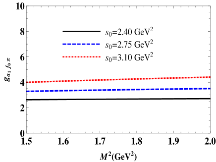
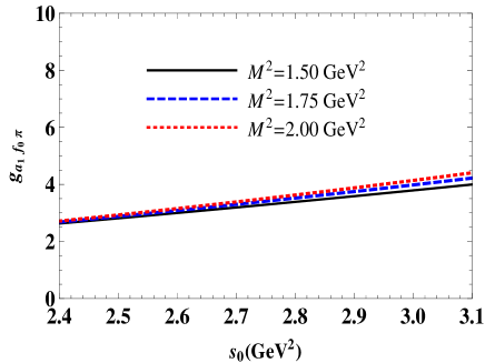
Figure 3: Dependence of the strong coupling $g_{a_{1}f_{0}\pi}$ on the Borel parameter $M^{2}$ at fixed $s_{0}$ (left panel), and on the continuum threshold $s_{0}$ at fixed $M^{2}$ (right panel).

IV The decay modes $a_{1}(1420)\to K^{\ast\pm}K^{\mp}$, $K^{\ast 0}\bar{K}^{0}$ and $\ \bar{K}^{\ast 0}K^{0}$

In this Section we concentrate on S-wave decays of the $a_{1}(1420)$ state. To this end we calculate strong couplings $g_{a_{1}K^{\ast}K^{-}}$ , $g_{a_{1}K^{\ast}K^{+}}$ and other two ones corresponding to vertices $a_{1}K^{\ast 0}\bar{K}^{0}$ and $\ a_{1}\bar{K}^{\ast 0}K^{0}$. All of these vertices are built of a tetraquark and two conventional mesons. Therefore, for their exploration, the light-cone sum rule approach has to be accompanied by the method of the soft meson approximation. This means that in order to satisfy the four-momentum conservation at these vertices momentum of a final light meson, for instance, the momentum of $K^{-}$ in $a_{1}K^{\ast+}K^{-}$ should be set $q=0$, which leads to important consequences for a calculational scheme: The distinctive features of the soft approximation are explained below.

Let us start from decay mode $a_{1}\rightarrow K^{\ast+}K^{-}$ that can be explored by means of the correlation function

$$\Pi_{\mu\nu}(p,q)=i\int d^{4}xe^{ip\cdot x}\langle K^{-}(q)|\mathcal{T}\{J_{\mu}^{K^{\ast+}}(x)J_{\nu}^{\dagger}(0)\}|0\rangle,$$ (41)

where $J_{\mu}^{K^{\ast+}}(x)$ is the correlation function of the $K^{\ast+}$ meson and has following form

$$J_{\mu}^{K^{\ast+}}(x)=\overline{s}(x)\gamma_{\mu}u(x).$$ (42)

Following standard prescriptions we write $\Pi_{\mu\nu}(p,q)$ in terms of physical parameters of the particles $a_{1},\ K^{\ast+}$ and $K^{-}$

$$\Pi_{\mu\nu}^{\mathrm{Phys}}(p,q)=\frac{\langle 0|J_{\mu}^{K^{\ast+}}|K^{\ast+}(p)\rangle}{p^{2}-m_{K^{\ast}}^{2}}\langle K^{\ast+}\left(p\right)K^{-}(q)|a_{1}(p^{\prime})\rangle$$

$$\times\frac{\langle a_{1}(p^{\prime})|J_{\nu}^{\dagger}|0\rangle}{p^{\prime 2}-m_{a_{1}}^{2}}+...,$$ (43)

where $p^{\prime}$ and $p$, $q$ are momenta of the initial and final particles. In Eq. (43) by dots we show contributions of excited resonances and continuum states. Further simplification of $\Pi_{\mu\nu}^{\mathrm{Phys}}(p,q)$ is achieved by utilizing the matrix elements:

$$\langle 0|J_{\mu}^{K^{\ast+}}|K^{\ast+}(p)\rangle=f_{K^{\ast}}m_{K^{\ast}}\varepsilon_{\mu},$$

$$\langle K^{\ast+}\left(p\right)K^{-}(q)|a_{1}(p^{\prime})\rangle=g_{a_{1}K^{\ast}K^{-}}\left[(p\cdot p^{\prime})(\varepsilon^{\ast}\cdot\varepsilon^{\prime})\right.$$

$$\left.-(p\cdot\varepsilon^{\prime})(p^{\prime}\cdot\varepsilon^{\ast})\right].$$ (44)

First of them, i.e. $\langle 0|J_{\mu}^{K^{\ast+}}|K^{\ast+}(p)\rangle$ is expressed in terms of $K^{\ast+}$ meson’s mass $m_{K^{\ast}}$ , decay constant $f_{K^{\ast}}$ and polarization vector $\varepsilon_{\mu}$. The second matrix element is written down using the strong coupling $g_{a_{1}K^{\ast}K^{-}}$ that should be evaluated from sum rules. In the soft limit $q\rightarrow 0$ we get $p^{\prime}=p$, as a result have to perform one-variable Borel transformation, which leads to

$$\mathcal{B}\Pi_{\mu\nu}^{\mathrm{Phys}}(p)=g_{a_{1}K^{\ast}K^{-}}m_{K^{\ast}}m_{a_{1}}f_{K^{\ast}}f_{a_{1}}\frac{e^{-m^{2}/M^{2}}}{M^{2}}$$

$$\times\left(m^{2}g_{\mu\nu}-p_{\nu}p_{\mu}^{\prime}\right)+\ldots,$$ (45)

where

$$m^{2}=\frac{m_{K^{\ast}}^{2}+m_{a_{1}}^{2}}{2}.$$ (46)

We keep in Eq. (45) $p_{\nu}\neq p_{\mu}^{\prime}$ to demonstrate explicitly its Lorentz structures. Contributions of higher resonances and continuum states are denoted in Eq. (45) by dots: Some of them are not suppressed even after the Borel transformation. Unsuppressed terms correspond to vertices containing excited states of involved particles. This is an advantage when one is interested in decays of excited tetraquarks to conventional ground-state mesons or their decays to final excited mesons. But it emerges as a problem if one considers only ground-state vertices. In other words, in the soft limit the phenomenological side of sum rules takes a complicated form which is one of aforementioned properties of this approximation Belyaev:1994zk .

In the soft limit the correlation function $\Pi_{\mu\nu}^{\mathrm{OPE}}(p)$ is given by the formula

$$\Pi_{\mu\nu}^{\mathrm{OPE}}(p)=i\int d^{4}xe^{ipx}\frac{\epsilon\widetilde{\epsilon}}{\sqrt{2}}\left\{\left[\gamma_{5}\widetilde{S}_{u}^{ic}(x){}\gamma_{\mu}\widetilde{S}_{s}^{bi}(-x){}\gamma_{\nu}\right]\right.$$

$$\left.+\left[\gamma_{\nu}\widetilde{S}_{u}^{ic}(x)\gamma_{\mu}\widetilde{S}_{s}^{bi}(-x)\gamma_{5}\right]\right\}_{\alpha\beta}\langle K^{-}(q)|\overline{s}_{\alpha}^{e}(0)u_{\beta}^{a}(0)|0\rangle,$$

where $\epsilon\widetilde{\epsilon}=\epsilon^{dab}\epsilon^{dec}$ . As is seen,  $\Pi_{\mu\nu}^{\mathrm{OPE}}(p)$ depends only on local matrix elements of $K^{-}$ meson.

Contribution to the correlation function comes from the matrix element

$$\langle 0|\overline{u}(0)i\gamma_{5}s(0)|K\rangle=f_{K}\mu_{K},$$ (48)

where $\mu_{K}=m_{K}^{2}/(m_{s}+m_{u})$. The function $\Pi_{\mu\nu}^{\mathrm{OPE}}(p)$ contains the same Lorentz structures as its phenomenological counterpart (45). We work with invariant amplitudes $\sim g_{\mu\nu}$, and our result for the Borel transform of the relevant invariant function $\Pi^{\mathrm{OPE}}(p^{2})$ reads

$$\Pi^{\mathrm{OPE}}(M^{2})=\int_{4m_{s}^{2}}^{\infty}ds\rho^{\mathrm{pert.}}(s)e^{-s/M^{2}}+\frac{f_{K}\mu_{K}}{\sqrt{2}}$$

$$\times\left[\frac{m_{s}}{6}\left(2\langle\overline{u}u\rangle-\langle\overline{s}s\rangle\right)\right.+\frac{1}{72}\langle\frac{\alpha_{s}G^{2}}{\pi}\rangle$$

$$\left.+\frac{m_{s}}{36M^{2}}\langle\overline{s}g_{s}\sigma Gs\rangle-\frac{g_{s}^{2}}{243M^{2}}\left(\langle\overline{s}s\rangle^{2}+\langle\overline{u}u\rangle^{2}\right)\right],$$ (49)

where

$$\rho^{\mathrm{pert.}}(s)=\frac{f_{K}\mu_{K}}{12\sqrt{2}\pi^{2}}s.$$

In Eq. (49) the spectral density $\rho^{\mathrm{pert.}}(s)$ is found from the imaginary part of the relevant piece in the correlation function, whereas the Borel transform of other terms are calculated directly from $\Pi^{\mathrm{OPE}}(p^{2})$. The function $\Pi^{\mathrm{OPE}}(M^{2})$ contains terms up to dimension six and has a rather compact form. It is evident that the soft approximation considerably simplifies the correlation function $\Pi^{\mathrm{OPE}}(p^{2})$ , which is another peculiarity of the method.

The sum rule for the strong coupling $g_{a_{1}K^{\ast}K^{-}}$ should be obtained from the equality

$$g_{a_{1}K^{\ast}K^{-}}m_{K^{\ast}}m_{a_{1}}f_{K^{\ast}}f_{a_{1}}m^{2}\frac{e^{-m^{2}/M^{2}}}{M^{2}}+...=\Pi^{\mathrm{OPE}}(M^{2}).$$ (50)

But before performing the standard continuum subtraction one needs to remove unsuppressed terms from the left-hand side of this equality. This task is solved by acting on both sides of Eq. (50) by the operator Belyaev:1994zk ; Ioffe:1983ju

$$\mathcal{P}(M^{2},m^{2})=\left(1-M^{2}\frac{d}{dM^{2}}\right)M^{2}e^{m^{2}/M^{2}},$$

that singles out the ground-state term. Remaining contributions can be subtracted afterwards in a usual manner, which requires the replacing (10) in the first term of  $\Pi^{\mathrm{OPE}}(M^{2})$ while leaving components $\sim(M^{2})^{0}$ and $\sim 1/M^{2}$ in their original forms Belyaev:1994zk .

The width of the decay $a_{1}\rightarrow K^{\ast+}K^{-}$ is given by the following expression

$$\Gamma(a_{1}\rightarrow K^{\ast+}K^{-})=\frac{g_{a_{1}K^{\ast}K^{-}}^{2}m_{K^{\ast}}^{2}}{24\pi}|\overrightarrow{p}|\left(3+\frac{2|\overrightarrow{p}|^{2}}{m_{K^{\ast}}^{2}}\right),$$

where now

$$|\overrightarrow{p}|=\frac{1}{2m_{a_{1}}}\left(m_{a_{1}}^{4}+m_{K^{\ast}}^{4}+m_{K}^{4}-2m_{K^{\ast}}^{2}m_{a_{1}}^{2}\right.$$

$$\left.-2m_{K}^{2}m_{a_{1}}^{2}-2m_{K^{\ast}}^{2}m_{K}^{2}\right)^{1/2}.$$ (51)

The obtained for $g_{a_{1}K^{\ast}K^{-}}$ sum rule can be easily adopted for numerical computations. The working windows for the parameters $M^{2}$ and $s_{0}$ used in the case of the $a_{1}\rightarrow f_{0}(980)\pi$ decay is suitable for $a_{1}\rightarrow K^{\ast+}K^{-}$ process, as well. The mass of mesons $K^{\ast+}$ and $K^{-}$ are taken from Ref. Patrignani:2016xqp

$$m_{K^{\pm}} = (493.677\pm 0.016)\ \ \mathrm{MeV},$$

$$m_{K^{\ast\pm}} = (891.76\pm 0.25)\ \mathrm{MeV}.$$ (52)

For their decay constants we use

$$f_{K^{\pm}} = (155.72\pm 0.51)\ \mathrm{MeV,}$$

$$f_{K^{\ast 0(\pm)}} = 225\ \mathrm{MeV.}$$ (53)

Results of calculations are presented below:

$$g_{a_{1}K^{\ast}K^{-}}=(2.84\pm 0.79)\ \mathrm{GeV}^{-1},$$

$$\Gamma(a_{1}\rightarrow K^{\ast+}K^{-})=(37.84\pm 10.97)\ \mathrm{MeV}.$$ (54)

The strong coupling $g_{a_{1}K^{\ast}K^{+}}$ and width of the decay $\Gamma(a_{1}\rightarrow K^{\ast-}K^{+})$ are also given by Eq. (54).

The analysis of the next two partial decay channels of the $a_{1}(1420)$ state $a_{1}\rightarrow K^{\ast 0}\bar{K}^{0}\left(\bar{K}^{\ast 0}K^{0}\right)$ does not differ from one presented in a detailed form in this section. Let us only write down masses of the $K^{0}(\bar{K}^{0})$ and $K^{\ast 0}(\bar{K}^{\ast 0})$ mesons

$$m_{K^{0}} = (497.611\pm 0.013)\ \mathrm{MeV},$$

$$m_{K^{\ast 0}} = (895.55\pm 0.20)~{}\mathrm{MeV,}$$ (55)

used in numerical computations. The decay constants of these pseudoscalar and vector mesons are taken equal to ones from Eq. (53). We omit further details and write down final sum rules’ predictions for these channels:

$$g_{a_{1}K^{\ast 0}\overline{K}^{0}}=(2.85\pm 0.82)\ \mathrm{GeV}^{-1},$$

$$\Gamma(a_{1}\rightarrow K^{\ast 0}\bar{K}^{0})=(33.35\pm 9.76)\ \mathrm{MeV}.$$ (56)

The obtained in the sections III and IV results for partial decays of the $a_{1}(1420)$ state enable us to calculate its full width: For $\Gamma$ we get

$$\Gamma=(145.52\pm 20.79)\text{ }\mathrm{MeV,}$$ (57)

which within theoretical errors of sum rule computations is compatible with the data provided by the COMPASS Collaboration.

V Concluding notes

The $a_{1}(1420)$ meson recently discovered by the COMPASS Collaboration took its place in an already overpopulated range of the light $a_{1}$ axial-vector mesons with $J^{PC}=1^{++}$ worsening a situation with their interpretation. The standard model of the mesons as bound states of a quark and a antiquark meets with difficulties to find a proper place for all of them. Thus, the $a_{1}(1420)$ meson can not be interpreted as the radial excitation of $a_{1}(1260)$, because the mass difference between them is small to accept this assumption. Explanations of $a_{1}(1420)$ as an dynamical effect observed in $a_{1}(1260)\rightarrow f_{0}(980)\pi$ decay are presented in the literature by number of works.

Alternative interpretations of the $a_{1}(1420)$ meson as a four-quark exotic state are among models in use, as well. In the framework of this approach it was considered as a pure diquark-antidiquark state or some admixture of a diquark-antidiquark and $q\overline{q}$ component. The molecular organization for $a_{1}(1420)$ was also employed in the literature.

In the present work we have treated the $a_{1}(1420)$ meson as a pure diquark-antidiquark state, and calculated its spectroscopic parameters, and widths of five decay modes. Our result for the mass of $a_{1}(1420)$ evaluated using QCD two-point sum rule method and given by $m_{a_{1}}=1416_{-79}^{+81}\ \ \mathrm{MeV}$ is in excellent agreement with the experimental result. It is also in accord within small computational errors with the prediction obtained in Ref. Chen:2015fwa . The full width of the $a_{1}(1420)$ meson has been calculated on basis of its five decay channels and led to $\Gamma=(145.52\pm 20.79)$ $\mathrm{MeV}$. By taking into account theoretical uncertainties of our calculations and experimental errors it agrees with measurements by the COMPASS Collaboration $\Gamma=153_{-23}^{+8}\ \mathrm{MeV}$.

Present studies have confirmed that the $a_{1}(1420)$ meson can be considered as a serious candidate to an exotic state, and a diquark-antidiquark model of its structure deserves detailed investigations.

Appendix A The light quark propagators and $\Pi_{\mathrm{V}}(M^{2},\ s_{0})$

The light quark propagator is necessary to find QCD side of the correlation functions in the mass and strong couplings’ calculations. In the present work for the light $q$-quark propagator $S_{q}^{ab}(x)$ we use the following formula

$$S_{q}^{ab}(x)=i\delta_{ab}\frac{\not{x}}{2\pi^{2}x^{4}}-\delta_{ab}\frac{m_{q}}{4\pi^{2}x^{2}}-\delta_{ab}\frac{\langle\overline{q}q\rangle}{12}+i\delta_{ab}\frac{\not{x}m_{q}\langle\overline{q}q\rangle}{48}-\delta_{ab}\frac{x^{2}}{192}\langle\overline{q}g_{s}\sigma Gq\rangle+i\delta_{ab}\frac{x^{2}\not{x}m_{q}}{1152}\langle\overline{q}g_{s}\sigma Gq\rangle$$

$$-i\frac{g_{s}G_{ab}^{\alpha\beta}}{32\pi^{2}x^{2}}\left[\not{x}{\sigma_{\alpha\beta}+\sigma_{\alpha\beta}}\not{x}\right]-i\delta_{ab}\frac{x^{2}\not{x}g_{s}^{2}\langle\overline{q}q\rangle^{2}}{7776}-\delta_{ab}\frac{x^{4}\langle\overline{q}q\rangle\langle g_{s}^{2}G^{2}\rangle}{27648}+\ldots$$ (A.58)

The propagator (A.58) has been used to calculate the correlation function $\Pi_{\mu\nu}^{\mathrm{OPE}}(p)$. Below we provide the subtracted Borel transform of $\Pi_{\mathrm{V}}(p^{2})$

$$\Pi_{\mathrm{V}}(M^{2},s_{0})=\frac{1}{2}\sum_{q=u,d}\left\{\int_{4m_{s}^{2}}^{s_{0}}dse^{-s/M^{2}}\left[\frac{s^{4}}{9\cdot 2^{12}\pi^{6}}+s^{2}\left(\frac{m_{s}(3\langle\overline{s}s\rangle-7\langle\overline{q}q\rangle)}{3\cdot 2^{7}\pi^{4}}+\frac{\langle G^{2}\rangle}{9\cdot 2^{9}\pi^{4}}\right)+s\left(\frac{5m_{s}^{2}\langle G^{2}\rangle}{9\cdot 2^{11}\pi^{4}}+\frac{5\langle\overline{s}s\rangle\langle\overline{q}q\rangle}{36\pi^{2}}\right.\right.\right.$$

$$\left.-\frac{m_{s}(4\langle\overline{q}g_{s}\sigma Gq\rangle-15\langle\overline{s}g_{s}\sigma Gs\rangle)}{9\cdot 2^{6}\pi^{4}}+\frac{g_{s}^{2}(\langle\overline{s}s\rangle^{2}+\langle\overline{q}q\rangle^{2})}{972\pi^{4}}\right)+\frac{m_{s}^{2}(\langle\overline{s}s\rangle^{2}-6\langle\overline{s}s\rangle\langle\overline{q}q\rangle+8\langle\overline{q}q\rangle^{2})}{48\pi^{2}}$$

$$\left.-\frac{\langle G^{2}\rangle m_{s}(\langle\overline{s}s\rangle+17\langle\overline{q}q\rangle)}{3\cdot 2^{9}\pi^{2}}-\frac{\langle G^{2}\rangle^{2}}{3\cdot 2^{10}\pi^{2}}-\frac{\langle\overline{s}g_{s}\sigma Gs\rangle\langle\overline{q}q\rangle}{8\pi^{2}}\right]-\frac{m_{s}\langle G^{2}\rangle(2\langle\overline{s}g_{s}\sigma Gs\rangle-27\langle\overline{q}g_{s}\sigma Gq\rangle)}{27\cdot 2^{9}\pi^{2}}$$

$$+\frac{2m_{s}(\langle\overline{s}s\rangle^{2}\langle\overline{q}q\rangle-2\langle\overline{q}q\rangle^{2}\langle\overline{s}s\rangle)}{9}+\frac{m_{s}g_{s}^{2}}{486\pi^{2}}\left[\langle\overline{s}s\rangle^{3}-2\langle\overline{s}s\rangle^{2}\langle\overline{q}q\rangle+2\langle\overline{s}s\rangle\langle\overline{q}q\rangle^{2}-2\langle\overline{q}q\rangle^{3}\right]+\frac{\langle\overline{s}g_{s}\sigma Gs\rangle\langle\overline{q}g_{s}\sigma Gq\rangle}{3\cdot 2^{4}\pi^{2}}$$

$$+\frac{\langle G^{2}\rangle\left(\langle\overline{s}s\rangle^{2}+25\langle\overline{s}s\rangle\langle\overline{q}q\rangle-2\langle\overline{q}q\rangle^{2}\right)}{27\cdot 2^{5}}+\frac{g_{s}^{2}\langle G^{2}\rangle\left(\langle\overline{s}s\rangle^{2}+\langle\overline{q}q\rangle^{2}\right)}{2^{4}\cdot 3^{6}\pi^{2}}+\frac{1}{M^{2}}\left[\frac{m_{s}\langle G^{2}\rangle^{2}(2\langle\overline{s}s\rangle+9\langle\overline{q}q\rangle)}{81\cdot 2^{10}}+\frac{2m_{s}\langle\overline{s}s\rangle^{2}\langle\overline{q}g_{s}\sigma Gq\rangle}{27}\right.$$

$$+\frac{g_{s}^{2}m_{s}(\langle\overline{s}g_{s}\sigma Gs\rangle-\langle\overline{q}g_{s}\sigma Gq\rangle)}{2^{3}\cdot 3^{6}\pi^{2}}\left(2\langle\overline{s}s\rangle^{2}-\langle\overline{s}s\rangle\langle\overline{q}q\rangle+3\langle\overline{q}q\rangle^{2}\right)+\frac{\langle G^{2}\rangle\langle\overline{s}g_{s}\sigma Gs\rangle\langle\overline{q}q\rangle}{432}$$

$$\left.\left.-\frac{g_{s}^{4}}{2^{4}\cdot 3^{7}\pi^{2}}\left(\langle\overline{s}s\rangle^{4}+4\langle\overline{s}s\rangle^{2}\langle\overline{q}q\rangle^{2}+\langle\overline{q}q\rangle^{4}\right)\right]\right\},$$ (A.59)

where we have used the notation

$$\langle G^{2}\rangle=\langle\frac{\alpha_{s}G^{2}}{\pi}\rangle.$$

In Section III we have used the light-cone propagators of the light $q=u$ and $s$ quarks. This propagator is determined by the formula

$$S_{q}^{ab}(x)=\frac{i\not{x}}{2\pi^{2}x^{4}}\delta_{ab}-\frac{m_{q}}{4\pi^{2}x^{2}}\delta_{ab}-\frac{\langle\overline{q}q\rangle}{12}\left(1-i\frac{m_{q}}{4}\not{x}\right)\delta_{ab}-\frac{x^{2}}{192}m_{0}^{2}\langle\overline{q}q\rangle\left(1-i\frac{m_{q}}{6}\not{x}\right)\delta_{ab}$$

$$-ig_{s}\int_{0}^{1}du\left\{\frac{\not{x}}{16\pi^{2}x^{2}}G_{ab}^{\mu\nu}(ux)\sigma_{\mu\nu}-\frac{iux_{\mu}}{4\pi^{2}x^{2}}G_{ab}^{\mu\nu}(ux)\gamma_{\nu}-\frac{im_{q}}{32\pi^{2}}G_{ab}^{\mu\nu}(ux)\sigma_{\mu\nu}\left[\ln\left(\frac{-x^{2}\Lambda^{2}}{4}\right)+2\gamma_{E}\right]\right\},$$ (A.60)

where $\gamma_{E}\simeq 0.577$ is the Euler constant and $\Lambda$ is the QCD scale parameter.

References

- (1) C. Patrignani et al. [Particle Data Group], Chin. Phys. C 40, 100001 (2016).
- (2) K. Chen, C. Q. Pang, X. Liu and T. Matsuki, Phys. Rev. D 91, 074025 (2015).
- (3) C. Adolph et al. [COMPASS Collaboration], Phys. Rev. Lett. 115, 082001 (2015).
- (4) R. L. Jaffe, Phys. Rev. D 15, 267 (1977).
- (5) J. D. Weinstein and N. Isgur, Phys. Rev. D 41, 2236 (1990).
- (6) M. G. Alford and R. L. Jaffe, Nucl. Phys. B 578, 367 (2000).
- (7) C. Amsler and N. A. Tornqvist, Phys. Rept. 389, 61 (2004).
- (8) D. V. Bugg, Phys. Rept. 397, 257 (2004).
- (9) E. Klempt and A. Zaitsev, Phys. Rept. 454, 1 (2007).
- (10) L. Maiani, F. Piccinini, A. D. Polosa and V. Riquer, Phys. Rev. Lett. 93, 212002 (2004).
- (11) G. ’t Hooft, G. Isidori, L. Maiani, A. D. Polosa and V. Riquer, Phys. Lett. B 662, 424 (2008).
- (12) J. I. Latorre and P. Pascual, J. Phys. G 11, L231 (1985).
- (13) S. Narison, Phys. Lett. B 175, 88 (1986).
- (14) T. V. Brito, F. S. Navarra, M. Nielsen and M. E. Bracco, Phys. Lett. B 608, 69 (2005).
- (15) Z. G. Wang and W. M. Yang, Eur. Phys. J. C 42, 89 (2005).
- (16) H. X. Chen, A. Hosaka and S. L. Zhu, Phys. Rev. D 76, 094025 (2007).
- (17) H. J. Lee, Eur. Phys. J. A 30, 423 (2006).
- (18) J. Sugiyama, T. Nakamura, N. Ishii, T. Nishikawa and M. Oka, Phys. Rev. D 76, 114010 (2007).
- (19) T. Kojo and D. Jido, Phys. Rev. D 78, 114005 (2008).
- (20) Z. G. Wang, Eur. Phys. J. C 76, 427 (2016).
- (21) Z. G. Wang, arXiv:1401.1134 [hep-ph].
- (22) H. X. Chen, E. L. Cui, W. Chen, T. G. Steele, X. Liu and S. L. Zhu, Phys. Rev. D 91, 094022 (2015).
- (23) T. Gutsche, V. E. Lyubovitskij and I. Schmidt, Phys. Rev. D 96, 034030 (2017).
- (24) M. Mikhasenko, B. Ketzer and A. Sarantsev, Phys. Rev. D 91, 094015 (2015).
- (25) X. H. Liu, M. Oka and Q. Zhao, Phys. Lett. B 753, 297 (2016).
- (26) F. Aceti, L. R. Dai and E. Oset, Phys. Rev. D 94, 096015 (2016).
- (27) J. L. Basdevant and E. L. Berger, Phys. Rev. Lett. 114, 192001 (2015).
- (28) W. Wang and Z. X. Zhao, Eur. Phys. J. C 76, 59 (2016).
- (29) T. Gutsche, M. A. Ivanov, J. G. Körner, V. E. Lyubovitskij and K. Xu, arXiv:1710.02357 [hep-ph].
- (30) M. A. Shifman, A. I. Vainshtein and V. I. Zakharov, Nucl. Phys. B 147, 385 (1979).
- (31) M. A. Shifman, A. I. Vainshtein and V. I. Zakharov, Nucl. Phys. B 147, 448 (1979).
- (32) I. I. Balitsky, V. M. Braun and A. V. Kolesnichenko, Nucl. Phys. B 312, 509 (1989).
- (33) V. M. Belyaev, V. M. Braun, A. Khodjamirian and R. Ruckl, Phys. Rev. D 51, 6177 (1995).
- (34) S. S. Agaev, K. Azizi and H. Sundu, Phys. Rev. D 93, 074002 (2016).
- (35) B. L. Ioffe and A. V. Smilga, Nucl. Phys. B 232, 109 (1984).
- (36) S. S. Agaev, K. Azizi and H. Sundu, Phys. Rev. D 95, 034008 (2017).
- (37) S. S. Agaev, K. Azizi and H. Sundu, Eur. Phys. J. C 77, 321 (2017).
- (38) S. S. Agaev, K. Azizi and H. Sundu, Phys. Rev. D 95, 114003 (2017).
- (39) S. S. Agaev, K. Azizi and H. Sundu, Phys. Rev. D 96, 034026 (2017).
- (40) S. S. Agaev, K. Azizi and H. Sundu, arXiv:1710.01971 [hep-ph].
- (41) V. M. Braun and I. E. Filyanov, Z. Phys. C 48, 239 (1990).
- (42) P. Ball, JHEP 9901, 010 (1999).
- (43) P. Ball, V. M. Braun and A. Lenz, JHEP 0605, 004 (2006).
- (44) S. S. Agaev, K. Azizi and H. Sundu, Phys. Rev. D 93, 114036 (2016).
- (45) S. S. Agaev, V. M. Braun, N. Offen and F. A. Porkert, Phys. Rev. D 83, 054020 (2011).
- (46) S. S. Agaev, V. M. Braun, N. Offen and F. A. Porkert, Phys. Rev. D 86, 077504 (2012).
- (47) V. M. Braun, S. Collins, M. Göckeler, P. Perez-Rubio, A. Schäfer, R. W. Schiel and A. Sternbeck, Phys. Rev. D 92, 014504 (2015).