Analysis of the anomalous mean-field like properties of Gaussian core model in terms of entropy

Abstract

Studies of the Gaussian core model (GCM) have shown that it behaves like a mean-field model and the properties are quite different from standard glass former. In this work, we investigate the entropies, namely the excess entropy ($S_{ex}$) and the configurational entropy ($S_{c}$) and their different components to address these anomalies. Our study corroborates most of the earlier observations and also sheds new light on the high and low temperature dynamics. We find that unlike in standard glass former where high temperature dynamics is dominated by two-body correlation and low temperature by many-body correlations, in GCM both high and low temperature dynamics are dominated by many body correlations. We also find that the many-body entropy which is usually positive at low temperatures and is associated with activated dynamics is negative in GCM suggesting suppression of activation. Interestingly despite suppression of activation the Adam-Gibbs (AG) relation which describes activated dynamics holds in GCM, thus suggesting a non-activated contribution in AG relation. We also find an overlap between the AG and mode coupling power law regime leading to a power law behaviour of $S_{c}$. From our analysis of this power law behaviour we predict that in GCM the high temperature dynamics will disappear at dynamical transition temperature and below that, there will be a transition to the activated regime. Our study further reveals that the activated regime in GCM is quite narrow.

I Introduction

On cooling a liquid sufficiently fast it does not get enough time to crystallize and enters the supercooled liquid state. On further cooling it becomes a glass. The manner in which such supercooled liquid becomes amorphous rigid solid is poorly understood. Numerous theories have been proposed to explain this slowing down of the dynamics in supercooled liquids usoft1 ; usoft2 ; usoft3 ; usoft4 but none of them have successfully answered all the questions. Mode coupling theory (MCT), known as the microscopic theory of glass transition is one such theory meanfield_gcm_kuni6 . According to the predictions of this theory, at the dynamical transition temperature, the relaxation time diverges in a power law manner gotze1999 ; GMCT_Reichman . This power law behaviour is indeed observed in many experiments and computer simulation studies du_mct_exp ; RFOT ; cavagna2001_epl ; sciortino-pre-2002 ; sciortino-saddle . However for these systems at low enough temperatures one observes a departure from the power law and the divergence predicted is thus avoided.

According to the random first order transition theory (RFOT), at the dynamical transition temperature the system is trapped in one of the basins of its rugged free energy landscape RFOT_cavagna . At the mean-field level, the system is permanently trapped in one such minima as the barriers between the minima become infinite and thus as predicted by MCT the dynamics is completely frozen. In finite dimensions the barrier heights are less, thus this transition predicted by MCT is suppressed by the activation process. At low temperatures the dynamics is governed by activation and relaxation time follows the well-known Adam-Gibbs (AG) relation adam-gibbs , which expresses relaxation time, $\tau$ in terms of a thermodynamic quantity, the configurational entropy $S_{c}$.

Although MCT like power law behaviour is found in simulation and experimental studies, thus predicting a transition temperature, $T_{c}$, the microscopic MCT when solved numerically using structural information from simulations, predicts a transition at $T_{c}^{micro}$ which is higher than $T_{c}$ GMCT_Reichman ; sciortino-pre-2002 . The reason for the prediction of this higher transition temperature is not fully understood. However it is believed that the Gaussian approximation made in the naive form of MCT role_pair which leads to the non-linear feedback mechanism is responsible for the higher value of $T_{c}^{micro}$. Also in a recent work we have shown that the form of the vertex function which depends on the structure factor might also be responsible for this premature divergence unravel .

As MCT is a microscopic mean-field theory, it is expected that the predictions made by MCT should systematically improve as we go towards mean-field like systems by increasing the dimension. It was found that for 4 dimensional hard sphere fluid, MCT predicts the slow dynamics much better than it does for lower dimensions 4d_mct . Another way of achieving mean-field effect is by making the interaction between the particles long range. Ikeda et al. have shown that the Gaussian core model (GCM) behaves more like a mean-field system ikeda2011slow ; ikeda_Japan . The discrepancy between $T_{c}$ and $T_{c}^{micro}$ is around $20\%$ for GCM whereas for standard glass former like Kob-Andersen (KA) model it is above $100\%$. There are also other observations where GCM was found to behave quite differently from standard glass forming systems meanfieldGCM . It has been observed that for most of the glass former, the MCT power law exponent $\gamma$ varies when it is obtained from power law fits of relaxation time and diffusion coefficient but for GCM these values come closer meanfieldGCM . In standard glass former as the system approaches low temperatures, both the non-Gaussian parameter $\alpha_{2}(t)$ and the four-point correlation function $\chi_{4}(t)$ increase in a similar fashion. However in GCM the $\alpha_{2}(t)$ was found to grow much less than in KA model ikeda2011slow but the $\chi_{4}(t)$ was found to grow much more meanfieldGCM . This apparent contradiction was explained in terms of mobility field. Large values of $\alpha_{2}(t)$ in KA model indicates large displacement of individual mobile particles whereas the enhancement of $\chi_{4}(t)$ in the GCM implies that this system has more cooperative motion. From mode localization analysis it has been found that as temperature decreases the unstable directions that disappear at the dynamic transition temperature are highly delocalized for the GCM whereas they are increasingly localized for other standard glass former like KA model meanfieldGCM_47 . It has been shown that due to the high energy barriers, the hopping like motions are strongly suppressed in GCM and the van Hove correlation function does not show any bimodal distribution even at low temperatures meanfieldGCM .

In this paper, we present a comparative study between KA binary mixture at density $\rho=1.2$ and mono-atomic GCM at $\rho=1.5$ and 2.0. Our study is based on the calculation of entropy and its separation into different components and studying its correlation with dynamics. We find that just like the other properties, the entropy and its components in GCM behave in a different way when compared to KA model. In our study, we show that both high and low temperature dynamics in GCM is dominated by many-body correlations and there is a suppression of activation. Surprisingly we find that even though there is a suppression of activation the AG relation is valid. We also find that there is an overlap between the AG and MCT regime and from our analysis we can predict that at a temperature, lower than that presented in this study the system makes a transition to activation dominated dynamics.

The paper is organized as follows: The simulation details for various systems are given in Sec. II. In the next section, we describe the methods used for evaluating various quantities and provide other necessary backgrounds. In Sec. IV, we present the results and discussions. Sec. V contains the conclusion.

II Simulation Details

In this study, we perform extensive molecular dynamics simulations of two different glass forming liquid models. One is the binary Kob-Andersen Lennard-Jones liquid kob and the other is a soft Gaussian core model ikeda2011slow . The first system is binary and the second is a monodisperse system. The total number density is fixed at $\rho=N/V$ with the total number of particles N (where $N=N_{A}+N_{B}$ for binary system) and system volume $V$. The molecular dynamics (MD) simulations are carried out using the LAMMPS package lammps . We perform the simulations in the canonical ensemble (NVT) using Nosé-Hoover thermostat. The time constant for Nosé-Hoover thermostat is taken to be 100 time steps. The sample is kept in a cubic box with periodic boundary condition. For all state points, three to five independent samples with run lengths $>$ 100$\tau$ ($\tau$ is the $\alpha$- relaxation time) are analyzed.

II.1 Binary mixture of Kob-Andersen Lennard-Jones particles

The most well-known model for glass forming liquids is Kob-Andersen model which is a binary mixture (80:20) kob . The interatomic pair potential between species $\alpha$ and $\beta$, with ${\alpha,\beta}=A,B$, $U_{\alpha\beta}(r)$ is described by a shifted and truncated Lennard-Jones potential, as given by:

$$U_{\alpha\beta}(r)=\begin{cases}U_{\alpha\beta}^{(LJ)}(r;\sigma_{\alpha\beta},\epsilon_{\alpha\beta})-U_{\alpha\beta}^{(LJ)}(r^{(c)}_{\alpha\beta};\sigma_{\alpha\beta},\epsilon_{\alpha\beta}),&r\leq r^{(c)}_{\alpha\beta}\\ 0,&r>r^{(c)}_{\alpha\beta}\end{cases}$$

where $U_{\alpha\beta}^{(LJ)}(r;\sigma_{\alpha\beta},\epsilon_{\alpha\beta})=4\epsilon_{\alpha\beta}[({\sigma_{\alpha\beta}}/{r})^{12}-({\sigma_{\alpha\beta}}/{r})^{6}]$ and $r^{(c)}_{\alpha\beta}=2.5\sigma_{\alpha\beta}$. Length, temperature and time are given in units of $\sigma_{AA}$, ${k_{B}T}/{\epsilon_{AA}}$ and $\surd({m_{A}\sigma_{AA}^{2}}/{\epsilon_{AA}})$, respectively. The interaction parameters for Kob-Andersen model are, $\sigma_{AA}$ = 1.0, $\sigma_{AB}$ =0.8 ,$\sigma_{BB}$ =0.88, $\epsilon_{AA}$ =1, $\epsilon_{AB}$ =1.5, $\epsilon_{BB}$ =0.5, $m_{A}$ = $m_{B}$=1.0. The integration time step is fixed at 0.005. System size is $N=500$, where $N_{A}=400$ and $N_{B}=100$ and the density of the system is $\rho=1.2$.

II.2 Gaussian core model

The Gaussian core model is a one-component system. The interaction potential is a Gaussian shaped repulsive potential. The potential is shifted and truncated at the cutoff $r^{(c)}=5\sigma$ and is given by:

$$U(r)=\begin{cases}\epsilon_{0}\exp[-(r/\sigma)^{2}]-\epsilon_{0}\exp[-(r^{(c)}/\sigma)^{2}],&r\leq r^{(c)}\\ 0,&r>r^{(c)}.\end{cases}$$ (1)

Length, temperature and time are given in units of $\sigma$, ${k_{B}T}/{\epsilon_{0}}$ and $\surd({m\sigma^{2}}/{\epsilon_{0}})$, respectively. The interaction parameters are $\sigma$ = 1.0, $\epsilon_{0}$ =1.0, $m$ =1.0. The integration time step is fixed at 0.2. System size is $N=3456$ and we choose two densities, $\rho=1.5$ and $\rho=2.0$ for our study.

III Definations

III.1 Relaxation time

The relaxation times are obtained from the decay of the overlap function, $q(t)$, using the definition $q(t=\tau)=1/e$. The overlap function $q(t)$ is defined as,

$$q(t)\approx\frac{1}{N}\left\langle\sum_{i=1}^{N}\Theta(\mid{\bf{r}}_{i}(t_{0})-{\bf{r}}_{i}(t+t_{0})\mid)\right\rangle$$

$$\Theta(x)=1,x\leq{\text{a implying “overlap”}}$$

$$=0,\text{otherwise}.$$ (2)

The cut off parameter ‘a’ is chosen as 0.3.

III.2 Excess Entropy

The thermodynamic excess entropy, $S_{ex}$, which arises due to structural correlations is the difference between the total entropy $S_{total}$ and the ideal gas value $S_{id}$ at the same state point (T,$\rho$). $S_{ex}$ is calculated by using the method described in Ref.sciortino2000thermodynamics . The entropy is first evaluated at a state point, usually at a high temperature and low density, where the system behaves like an ideal gas. Relative to this state point, entropy at any other state point can be calculated by using the combination of an isothermal and an isochoric path, avoiding any phase transition along this path. Along the isothermal path entropy change is given by,

$$S(T,V^{\prime})-S(T,V)=\frac{U(T,V^{\prime})-U(T,V)}{T}+\int_{V}^{V^{\prime}}\frac{P(V)}{T}dV,$$ (3)

and along the isochoric path it is,

$$S(T^{\prime},V)-S(T,V)=\int_{T}^{T^{\prime}}\frac{1}{T}\Big{(}\frac{\partial U}{\partial T}\Big{)}_{V}dT.$$ (4)

III.2.1 Pair and higher order excess entropy

By using Kirkwood factorization kirkwood of the N-particle distribution function green_jcp ; raveche ; Wallace , the excess entropy $S_{ex}$ can be expanded in an infinite series,

$$S_{ex}=\sum_{n=2}^{\infty}S_{n}=S_{2}+\Delta S,$$ (5)

$S_{n}$ are partial entropies which can be obtained by a suitable re-summation of spatial density correlations involving n-particle multiplets. The pair excess entropy $S_{2}$ for binary system reads as,

$$\frac{S_{2}}{k_{B}}=-2\pi\rho\sum_{\alpha\beta}x_{\alpha}x_{\beta}\int_{0}^{\infty}{g_{\alpha\beta}(r)\ln g_{\alpha\beta}(r)-[g_{\alpha\beta}(r)-1]}r^{2}dr,$$ (6)

where $g_{\alpha\beta}(r)$ is the atom-atom pair correlation function between type $\alpha$ and type $\beta$, $\rho$ is the density of the system, $x_{\alpha}$ is the mole fraction of type $\alpha$ and $k_{B}$ is the Boltzmann constant. $\Delta S=S_{ex}-S_{2}$, is called the residual multiparticle entropy (RMPE) which contains the higher order contributions (beyond two-body) to the excess entropy rmpe_saija1 .

III.3 Configurational Entropy

The configurational entropy ($S_{c}$ ) per particle, is calculated srikanth_PRL by subtracting the vibrational entropy from the total entropy of the system : $S_{c}(T)=S_{id}(T)+S_{ex}(T)-S_{vib}(T)$ shila-jcp ; Srikanth_nature . Here $S_{id}$ is the ideal gas entropy and the excess entropy, $S_{ex}$ is obtained by the method described in Sec. IIIB. For vibrational entropy we use a harmonic approximation to the potential energy about a given local minima. The detailed procedure for generating the local minima and calculating the vibrational entropy is given in Ref. srikanth_PRL ; shila-jcp ; Srikanth_nature . As mentioned in an earlier study meanfieldGCM in the calculation of the density of states, we also find some imaginary modes ($\sim 0.19\%$) which we ignore to calculate the vibrational entropy. We believe that this will not make any change in the physical properties of the system.

III.3.1 Pair Configurational Entropy

To obtain an estimate of the configurational entropy as predicted by the pair correlation we rewrite $S_{c}$ in terms of the pair contribution to configurational entropy, $S_{c2}$atreyee_prl ,

$$S_{c}=S_{id}+S_{ex}-S_{vib}=S_{id}+S_{2}+\Delta S-S_{vib}=S_{c2}+\Delta S.$$ (7)

Where $S_{c2}=S_{id}+S_{2}-S_{vib}$.

III.4 Mode coupling Theory

Mode coupling theory (MCT) is a well-known theory for glass forming liquids. This microscopic theory can qualitatively predict the dynamics of the glass forming liquid, if the structure of the liquid is known. Many experimental and simulation studies have proved that these predictions made by MCT are true gotze-jpcm-10A1 . The equation of motion for the intermediate scattering function is given by

$$\ddot{\bf{S}}(k,t)+{\bf{\Gamma}}\dot{\bf{S}}(k,t)+{\bf{\Omega}}_{k}^{2}{\bf{S}}(k,t)+{\bf{\Omega}}_{k}^{2}\int{\bf{\mathcal{M}}}(k,t-t^{\prime})\dot{\bf{S}}(k,t^{\prime})dt^{\prime}=0,$$ (8)

where ${\bf{\Omega}}_{k}^{2}=\frac{k^{2}k_{B}T}{m}{\bf{S(k)}}^{-1}$, ${\bf{S}}(k,t)$ is the matrix of intermediate scattering function $S_{\alpha\beta}(k,t)$ and memory function ${\bf{\mathcal{M}}}(k,t)$ can be written as :

$$[{\bf{\Omega}}^{2}_{k}{\bf{\mathcal{M}}}(k,t)]_{\alpha\beta} = \frac{1}{2\rho\sqrt{x_{\alpha}x_{\beta}}}\sum_{ll^{\prime}mm^{\prime}}\int\frac{d\bf{q}}{(2\pi)^{3}}V_{\alpha lm}({\bf{q,k-q}})$$ (9)

$$\times V_{\beta l^{\prime}m^{\prime}}({\bf{q,k-q}})S_{mm^{\prime}}({\bf{|k-q|}})$$

$$\times S_{ll^{\prime}}(q)\phi_{mm^{\prime}}(\mid{\bf{k-q}}\mid,t)\phi_{ll^{\prime}}(q,t),$$

where $\phi_{\alpha\beta}(k,t)=\frac{S_{\alpha\beta}(k,t)}{S_{\alpha\beta}(k,0)}$, ${\bf{k-q}}=\bf{p}$ and $V_{\alpha lm}({\bf{q}},{\bf{p}})=[\hat{\bf{k}}.{\bf{q}}\delta_{\alpha m}C_{\alpha l}(q)+\hat{\bf{k}}.{\bf{p}}\delta_{\alpha l}C_{\alpha m}(p)]$. ${\bf{C}}(k)$ is defined as ${\bf{S}}(k)^{-1}={\bf{1}}-{\bf{C}}(k)$. The static structure factors, $S_{\alpha\beta}(k)$ are calculated from simulation and are defined as,

$$S_{\alpha\beta}(k)=\frac{1}{\sqrt{N_{\alpha}N_{\beta}}}\sum_{i=1}^{N_{\alpha}}\sum_{j=1}^{N_{\beta}}\exp(-i{\bf{k}}.({\bf{r}}_{i}^{\alpha}-{\bf{r}}_{j}^{\beta})).$$ (10)

Solving Eq.(8) we can obtain the relaxation time from the decay of $\phi_{\alpha\beta}(k,t)$. The temperature dependence of the relaxation time provides us the information of the transition temperature $T_{c}^{micro}$.

IV Results and Discussions

As mentioned in the Introduction, many properties of the GCM are different from the conventional glass forming liquids like KA model ikeda2011slow ; ikeda_Japan ; meanfieldGCM and they appear more mean-field like. Here we present a comparative study between the GC and KA models like it has been done before. However, our analysis primarily focuses on the thermodynamic properties like the excess entropy and the configurational entropy and their components like pair and higher order terms. We also study the correlation between entropy and dynamics.

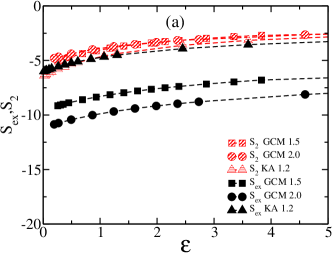
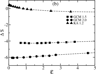
Figure 1: (a) $S_{ex}$ and $S_{2}$ are plotted as a function of temperature for GCM at $\rho=1.5$ and 2.0 and KA model at $\rho=1.2$. As the temperature range for GCM and KA model are very different, to make a meaningful comparison we plot these entropies against $\varepsilon=(\frac{T}{T_{c}}-1)$. In KA model there is a crossing between $S_{ex}$ and $S_{2}$. (b) $\Delta S$ against temperature for the same models. Only for KA model $\Delta S$ has positive contribution.

IV.1 Excess entropy

First, we study the excess entropy and its different components, the pair, $S_{2}$ and the higher order terms, $\Delta S$ (Sec. IIIB1, Eq. 5). Our study reveals that unlike in KA model where there is a clear separation of major contribution to high temperature MCT like dynamics and low temperature activated dynamics from the pair and higher order terms of the entropy respectively atreyee_prl ; prl_long ; onset ; unravel , in GCM that separation does not exist. We plot the $S_{ex}$ and $S_{2}$ for both KA and GC models as a function of temperature and observe certain stark differences between them. Since the temperature range for GCM and KA model are very different, to make a meaningful comparison, in the x-axis, we plot $\varepsilon=(\frac{T}{T_{c}}-1)$(Fig. 1). Unlike in KA and other simple glass forming liquids where at high temperature $S_{2}$ contributes to $80\%$ of $S_{ex}$, in GCM we find that even at temperature $T\simeq 10\times T_{c}$ the dynamics is dominated by $\Delta S$ and contribution of $S_{2}$ is only $34\%$ for $\rho=1.5$ and $29\%$ for $\rho=2.0$ (Table-1). Thus it implies that in GCM many-body correlations dominate the dynamics even at high temperatures and this contribution increases with density. Note that earlier studies have shown that the unstable modes which are characteristics of high temperature dynamics and disappear at $T_{c}$ are delocalized for GCM whereas they are localized for KA model meanfieldGCM . This can be explained from our entropy calculation. At high temperatures dominance of many-body correlation in GCM implies delocalized mode whereas dominance of pair correlation in KA model implies localized mode. Large absolute value of $\Delta S$ in GCM also suggests strong cooperative motion and can be connected to the earlier findings of larger value of $\chi_{4}$ when compared to KA model meanfieldGCM .

Table 1: $S_{ex}$, $S_{2}$ and $\Delta S$ at high temperature where $T\sim 10\times T_{c}$. In KA model $S_{2}$ contributes to $80\%$ of $S_{ex}$, whereas in GCM at $\rho=1.5$ it is $34\%$ and at $\rho=2.0$ the contribution is $29\%$.

	$T_{c}$	$T\sim 10\times T_{c}$	$S_{ex}$	$S_{2}$	$\Delta S$	$\frac{S_{2}}{S_{ex}}\%$
KA	0.435	5.00	-2.62092	-2.14422	-0.4767	82
GCM ($\rho=1.5$)	2.07$\times 10^{-5}$	2.00$\times 10^{-4}$	-5.73985	-1.96565	-3.7742	34
GCM ($\rho=2.0$)	2.68$\times 10^{-6}$	3.00$\times 10^{-5}$	-7.04557	-2.05902	-4.9866	29

In KA model with decrease in temperature the $S_{2}$ and $S_{ex}$ undergo a crossing and the many-body contribution to the entropy becomes positive. Recently we have shown that this crossing marks the onset temperature onset and the positive value of $\Delta S$ is associated with the activated dynamics as it leads to the increase in entropy and thus speed up of dynamics onset ; atreyee_prl ; unravel . Here we find that in GCM, $S_{2}$ and $S_{ex}$ never undergo a crossing and $\Delta S$ is never positive (Fig. 1). Thus we cannot predict an onset temperature from the entropy. It has been earlier observed that for hard sphere system in higher dimensions $\Delta S$ remains negative for a wider density regime truskett_2008 . In 3D, $\Delta S=0$ (marking a transition from negative to positive value) at the freezing density whereas in 4D the density where $\Delta S=0$ is higher than the freezing density and in 5D the $\Delta S$ remains negative much above the freezing density and the absolute value is much higher than that obtained for 3D and 4D systems. Similar difference between freezing point and $\Delta S=0$ point has also been observed in GCM rmpe_saija2 . These studies reveal that as we go to mean-field like systems the negative value of $\Delta S$ persists for a wider range of density or temperature and the absolute value of $\Delta S$ increases. Hence the fact that $\Delta S$ has a large negative value in GCM supports the earlier findings that GCM exhibits mean-field like behaviour meanfieldGCM usually observed in higher dimensional systems.

As mentioned before in our earlier study we have connected the positive value of $\Delta S$ to the activated dynamics atreyee_prl ; prl_long ; unravel . The positive value of $\Delta S$ implies higher order correlations increase the entropy, similarly activated dynamics which is many-body in nature is supposed to allow the system to explore more configurational space. Thus a negative value of $\Delta S$ in GCM predicts suppression of activation. This suppression of activation has already been reported by Coslovich et al. where they have shown that in GCM the van Hove correlation function ($G_{s}(r,t)$) does not show any bimodal distribution even at very low temperatures, which implies no hopping like motion meanfieldGCM . They have claimed that in the landscape picture this is due to the higher value of energy barriers meanfieldGCM .

To summaries, $\Delta S$ in KA model has small values and undergoes a sign change whereas absolute value of $\Delta S$ in GCM is large and remains negative. Thus many-body correlation in KA model is weak and it contributes primarily at low temperatures to the activated dynamics. In contrast, many-body correlation is strong in GCM, has contribution both at high and low temperature regimes but it primarily contributes to slowing down of the dynamics. It is possible that there can be some parts of the many-body contribution which speeds up the dynamics and some parts which slows it down as reported by Coslovich et al. meanfieldGCM where they have found the presence of both cooperative and incoherent many-body modes meanfieldGCM . However in the present study such separation in the calculation of $\Delta S$ is not possible.

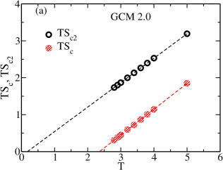
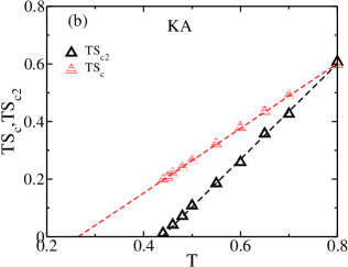
Figure 2: (a) Temperature dependence of $TS_{c}$ and $TS_{c2}$ for GCM at $\rho=2.0$. Both show linear behaviour. The Kauzmann temperature, $T_{K}$ and pair Kauzmann temperature, $T_{K2}$ obtained from the extrapolation of the lines. To plot $TS_{c}$ and $TS_{c2}$ in the same figure, we have divided $TS_{c2}$ by 10. (b) Same as in (a) but for the KA model. In GCM the two lines run almost parallel and $T_{K2}<T_{K}$, whereas in KA model the slopes are different, the lines cross each other and $T_{K2}>T_{K}$.

IV.2 Configurational entropy

Next we study the different contributions to the configurational entropy, $S_{c}$. Since this calculation is time consuming, for GCM we concentrate only at $\rho=2.0$. Note that for glass forming systems $TS_{c}$ vs T is found to be linear srikanth ; atreyee_prl ; prl_long and the extrapolation of the linear fit gives us a measure of the Kauzmann temperature, $T_{K}$ where the extrapolated $S_{c}$ vanishes. In our earlier work we have shown that $TS_{c2}$ vs T also shows a linear behaviour and predicts a transition temperature, $T_{K2}$ where the $S_{c2}$ vanishes unravel ; role_pair . In Fig. 2a and 2b we plot the $TS_{c}$ and $TS_{c2}$ against temperature both for GC and KA models respectively. We find that similar to KA model the $TS_{c}$ and $TS_{c2}$ vs T plots in GCM are linear. However, the main difference is that in GCM the two lines run almost parallel and $T_{K2}<T_{K}$, whereas in KA model the slopes are different, the lines cross each other and $T_{K2}>T_{K}$. This is related to the observation mentioned before (Fig. 1a) that in GCM, $S_{2}$ and $S_{ex}$ do not cross but in KA model they cross at the onset temperature. For conventional glass forming liquids like KA model atreyee_prl ; unravel ; role_pair we have also reported that $T_{K2}\simeq T_{c}$. In case of GCM $T_{K2}<<T_{c}$. The possible explanation for this is that $T_{c}$ marks the disappearance of high temperature dynamics. For systems where $S_{2}$ provides a dominant contribution at high temperatures the corresponding configurational entropy vanishes at $T_{c}$. This does not appear to be the case in GCM. As discussed before the high temperature non-activated dynamics in this system is dominated not by the pair but by the many-body correlations. Thus the disappearance of the high temperature dynamics around $T_{c}$ has no connection with the vanishing of the $S_{c2}$ and hence $T_{K2}\neq T_{c}$.

IV.3 Adam-Gibbs relation

As discussed in the Introduction it is believed that the low temperature dynamics for glass forming liquids is activated in nature and the relaxation time, $\tau$ is related to the configurational entropy, $S_{c}$ via AG relation:

$$\tau(T)=\tau_{o}\exp\left(\frac{A}{TS_{c}}\right),$$ (11)

where A is the AG coefficient. Since the GCM shows a suppression of activation ikeda2011slow ; meanfieldGCM we expect the AG relation to be violated in this system. To our surprise we find that in GCM the AG prediction of connection between dynamics and entropy holds as shown in Fig. 3a. This is the first time it is shown that for systems where activated dynamics is clearly suppressed the AG relation holds. In our earlier study we have already shown that AG relation holds not only at low temperatures where activated dynamics is dominant but also at reasonably high temperature, where the dynamics is still described by MCT unravel . Thus we claimed that there exists a non-activated contribution to AG and our present finding supports this argument. Note that in an earlier study it has been shown that in the 4D system AG relation holds but there has been no discussion about the suppression of activated dynamics shila_4d .

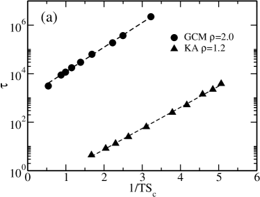
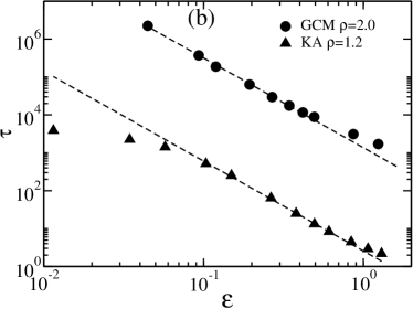
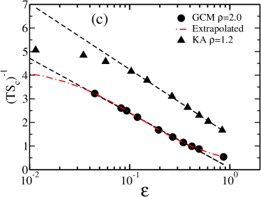
Figure 3: Comparative study of GCM at $\rho=2.0$ and KA model at $\rho=1.2$. (a) Adam Gibbs plot for the relaxation time ($\tau$ vs $\frac{1}{TS_{c}}$). Both follow AG relation. (b) The MCT power-law behaviour of relaxation time, $\tau$ vs $\varepsilon$ where $\varepsilon=(\frac{T}{T_{c}}-1)$. The dashed lines are MCT fit ($\tau\propto(T-T_{c})^{-\gamma}$). (c) $(TS_{c})^{-1}$ against $\varepsilon$. The dashed lines are MCT like power-law fit (Eq. (12)). The dashed-dot line is the extrapolated value of $(TS_{c})^{-1}$ obtained from Fig. 2a. For better comparison in GCM model $(TS_{c})^{-1}$ is multiplied by $10^{-6}$. We find that in (b) the relaxation time, $\tau$ and in (c) $(TS_{c})^{-1}$ follow power-law behaviour in the same temperature regime. However for GCM when compared to KA model this regime is shifted to lower temperatures. For GCM the simulated values of $\tau$ and $(TS_{c})^{-1}$ do not show any departure from power law. The extrapolated $(TS_{c})^{-1}$ (shown in (c)) can predict a departure from power law and a transition to activation dominated dynamics.

IV.4 AG and MCT overlap regime

In order to further understand this non-activated contribution to AG, we analyze the MCT power law behaviour of the relaxation time and the configurational entropy. In Fig.3b we plot the relaxation time for GCM and KA models. As reported earlier, like KA model the relaxation time, $\tau$ of GCM follows MCT like power law behaviour and predicts a transition temperature $T_{c}$ (Table-2). For most of the glass forming liquids like KA model the range of this regime is $0.1<(\frac{T}{T_{c}}-1)<1.0$ unravel . In contrast the power law regime in GCM is shifted towards lower temperatures. For GCM we do not find any deviation from MCT power law till the temperature we have studied ($(\frac{T}{T_{c}}-1)\simeq 0.0448$). Thus from this figure we cannot comment if the MCT divergence is real or avoided. Note that according to microscopic MCT calculation this power law regime appears at a lower temperature szamel-pre . It will be interesting to understand if this shift is also a mean-field effect. But this is beyond the scope of the present study.

Although fitting relaxation time and diffusion coefficient to MCT power law behaviour is done routinely, the study of the power law behaviour of the configurational entropy is not a standard protocol. In a recent work on KA model we have shown that there is an overlap between AG and MCT regime unravel . In this common regime we can write,

$$\frac{A}{TS_{c}}\propto\ln(\frac{T}{T_{c}}-1).$$ (12)

Thus the study of the power law behaviour of $(TS_{c})^{-1}$ is the best way to understand this regime. We find that similar to KA model in GCM there is an overlap between AG and MCT regime. Like in KA model the $(TS_{c})^{-1}$ vs $\ln(\frac{T}{T_{c}}-1)$ in GCM follows a linear behaviour (Fig. 3c). However unlike KA model and similar to what we observe for the relaxation time, this region is shifted to a lower temperature (Fig. 3b).

A consequence of the validity of both AG and MCT relation is that both $TS_{c}$ vs. T and $(TS_{c})^{-1}$ vs $\ln(\frac{T}{T_{c}}-1)$ show a linear behaviour. The former linear behaviour predicts a vanishing of $S_{c}$ at $T_{K}$ and the latter predicts that it vanishes at $T_{c}$. In KA model we have shown that these two contradicting behaviour appears because a part of $S_{c}$ vanishes at $T_{c}$ and is responsible for the predicted divergence like behaviour at $T_{c}$. Interestingly this part of the entropy, namely the pair part is connected to the high temperature dynamics. The other part of $S_{c}$, ie. $\Delta S$ survives and provides a finite value to $S_{c}$ below $T_{c}$. This makes the divergence at $T_{c}$ an avoided one and leads to the departure from linearity of the $(TS_{c})^{-1}$ vs $\ln(\frac{T}{T_{c}}-1)$ plot (Fig. 3c). This departure also marks a transition to an activation dominated regime, although the onset of activation happens at a higher temperature, $T_{onset}$ onset . Note that similar to KA model in GCM we find both $TS_{c}$ vs T and $(TS_{c})^{-1}$ vs $\ln(\frac{T}{T_{c}}-1)$ to be linear, thus predicting two vanishing temperatures for $S_{c}$, one at $T_{K}$ and the other at $T_{c}$, respectively. Till the lowest temperature studied here we do not find any departure from linearity of the $(TS_{c})^{-1}$ vs $\ln(\frac{T}{T_{c}}-1)$ plot. Thus we can not comment if the transition at $T_{c}$ is real or avoided. However if we plot the extrapolated value of $TS_{c}$ as obtained from Fig. 3a, we find that $(TS_{c})^{-1}$ vs $\ln(\frac{T}{T_{c}}-1)$ shows a departure from linearity (Fig. 3c). If we trust the extrapolation if not till $T_{K}$ but at least till some temperature which is lower than that studied here, then this departure implies two things. First, not the whole $S_{c}$ but some components of $S_{c}$, most probably the ones related to the high temperature dynamics vanishes at $T_{c}$ and second, at some temperature above $T_{c}$, the remaining part of $S_{c}$ becomes positive suggesting the presence of activation and around $T_{c}$ the activated dynamics becomes dominant. Note that unlike in KA model in GCM it is not the pair part of $S_{c}$ that vanishes at $T_{c}$. As mentioned before, this is because $S_{2}$ is not the dominant contributor to high temperature dynamics. From the present study we cannot specify till what order in $S_{ex}$ contributes to high temperature dynamics. However the departure from linearity seen in Fig. 3c and thus the prediction of a transition to activated dynamics around $T_{c}$ is similar to the earlier observations atreyee_prl ; unravel ; role_pair .

IV.5 Activation dominated regime

Next we show that our study further reveals that the activation dominated regime in GCM is very small. In Table-2 we have given the $T_{c}$, $T_{K}$ and also $T_{VFT}$ values, where $T_{VFT}$ is obtained from fitting $\tau$ to $\tau\sim\tau_{0}exp\left[\frac{1}{K_{VFT}(T/T_{VFT}-1)}\right]$ form. We have also tabulated the $\frac{T_{c}-T_{K}}{T_{K}}\%$ and $\frac{T_{c}-T_{VFT}}{T_{VFT}}\%$ values for KA and GCM systems. First we find that $T_{K}$ and $T_{VFT}$ are very close which is a reflection of the validity of the AG relation srikanth . We also find that the difference between $T_{c}$ and $T_{K}$/ $T_{VFT}$ is much smaller in GCM than in KA model (Table-2). This implies that the activation dominated regime in GCM is much smaller than that in KA model. Although our study predicts a transition to activated dynamics and that the regime of activated dynamics to be small it can not predict the degree of contribution of the activation to the total dynamics.

Figure 4: The power law dependence of $(D_{0}\tau_{mfpt})^{-1}$ predicts a transition temperature $T_{mfpt}$, which is close to the $T_{c}$ in scaled unit. The dashed line is the power law fit.

Table 2: The values for different dynamic and thermodynamic transition temperatures for KA at $\rho=1.2$ and GCM at $\rho=2.0$. $T_{K}\simeq T_{VFT}$ implies AG relation is valid. $\frac{T_{c}-T_{K}}{T_{K}}\%$ and $\frac{T_{c}-T_{VFT}}{T_{VFT}}\%$ are less for GCM suggesting narrow activation dominated regime.

	$KA(LJ\rho=1.2)$	$GCM(\rho=2.0)$
$T_{c}$	0.435	2.68$\times 10^{-6}$
$T_{K}$	0.27	2.36 $\times 10^{-6}$
$T_{VFT}$	0.28	2.31$\times 10^{-6}$
$T_{mfpt}$	0.428$\pm$ 0.022	2.66$\pm$ 0.01
$\frac{T_{c}-T_{K}}{T_{K}}\%$	61.11$\%$	13.56$\%$
$\frac{T_{c}-T_{VFT}}{T_{VFT}}\%$	55.36$\%$	16.02$\%$

IV.6 Mean-field theory (MFT) approach

Recently we have developed a mean-field like theory which can describe the dynamics of a collection of interacting particles in terms of a collection of non-interacting particles in an effective potential role_pair . The effect of the interaction between the particles are absorbed in this effective potential at a mean-field level. Below we provide a sketch of the derivation with few important equations. The details are given in Ref. role_pair . Starting from the Fokker-Planck equation we derived the Smoluchowski equation with an effective potential $\Phi(r)$. Using the dynamic density functional approach ramakrishnan-yossuf we obtained the effective caging potential as,

$$\Phi(r)=-\frac{1}{2}\int\frac{d{\bf q}}{(2\pi)^{3}}\rho C^{2}(q)S(q)e^{-q^{2}r^{2}/3}.$$ (13)

Here $C(q)$ is the direct correlation function and $S(q)$ is the static structure factor of the liquid. Note that the caging potential depends only on the equilibrium pair correlation function. Next we calculated the mean first passage time, the time required to escape from the effective potential which leads to caging of the particles,

$$\tau_{mfpt}=\frac{1}{D_{0}}\int_{0}^{r_{max}}e^{\beta\Phi(y)}dy\int_{0}^{y}e^{-\beta\Phi(z)}dz,$$ (14)

where $D_{0}=k_{B}T/\zeta$ and $\zeta$ is the coefficient of the friction of the system and $r_{max}$ is the range of localization potential $\Phi(r)$. As done earlier for other glass forming liquids role_pair , we calculate the mean first passage time in GCM. Note that the range of temperatures in GCM is much smaller compared to standard glass forming systems. This leads to numerical problems in the calculation of $\tau_{mfpt}$ as the temperature is in the exponential. However we can scale the potential and temperature in such a way that the temperature range moves to higher values. For this part of the calculation, we run simulations where $\epsilon=10^{6}\epsilon_{0}$, the temperature and the time are scaled as $T=T\times 10^{6}$ and $\Delta t=\Delta t\times 10^{-3}$. Although the time scale changes, the static properties like radial distribution function, $g(r)$ and structure factor, $S(q)$ remain same as in the original system and dynamics gets appropriately scaled. In Fig. 4, we show that $\tau_{mfpt}$ follows a power law behaviour and the transition temperature $T_{mfpt}\simeq T_{c}$ in the scaled unit (Table-2). Note that for KA model and other systems $T_{mfpt}\simeq T_{K2}\simeq T_{c}$. For GCM as discussed before $T_{K2}$ is much smaller as $S_{2}$ is not the dominant contributor to the high temperature dynamics. However, we find that although $S_{2}$ cannot predict the full high temperature dynamics the present mean-field theory using the same pair correlation as used for the calculation of $S_{c2}$ can.

V conclusion

In this work we present a comparative study between the GC and KA models. The work is similar in spirit to that presented earlier by other groups where it was found that the dynamic properties in GCM are quite different from that in KA model and are more mean-field like ikeda2011slow ; ikeda_Japan ; meanfieldGCM . However, in this work, we focus on the calculation of the entropy and its components and the study of the correlation between entropy and dynamics. Our study supports the conclusions made in the earlier studies and also makes some new predictions.

The excess entropy which is the loss of entropy of the liquid due to its correlations can be broken up into pair and higher order terms green_jcp ; raveche ; Wallace . For standard glass former like KA model at high temperatures the pair part of the excess entropy ($S_{2}$) contributes to 80$\%$ of the total excess entropy ($S_{ex}$) atreyee_prl ; BORZSAK1992227 . Thus high temperature dynamics is dominated by two-body correlation. At high temperatures $S_{2}$ is larger than $S_{ex}$ but with decrease in temperature they undergo a crossing which marks the onset temperature onset . The RMPE ($\Delta S$) undergoes a sign change and also a role reversal atreyee_prl . For KA model we have observed that small negative values of $\Delta S$ at high temperatures has very little contribution to the dynamics whereas small positive value of $\Delta S$ has a large contribution to the low temperature dynamics and has been connected to activation atreyee_prl . In GCM the scenario is quite different. At high temperatures the contribution of $S_{2}$ to $S_{ex}$ is only $\sim 30\%$. Thus in GCM unlike in KA model the high temperature dynamics is dominated by many-body correlations. The $S_{2}$ in GCM is always higher than $S_{ex}$ and they do not undergo any crossing. Thus we cannot predict an onset temperature from entropy. The RMPE does not undergo a sign change and no role reversal. The absolute value of RMPE in GCM is much larger than that in KA model, thus predicting larger contribution of many-body correlations which is similar to the observation of high value of $\chi_{4}(t)$ in GCM meanfieldGCM . Also negative $\Delta S$ value predicts suppression of activated motion which has been reported earlier from the study of van Hove correlation function meanfieldGCM .

Although there is suppression of activation we find that the AG relation in GCM holds over a wide temperature regime. As far as our knowledge this is the first system where both suppression of activation and validity of AG relation is reported simultaneously. In our earlier study on KA model we suggested that observed overlap between AG and MCT regime implies that there is a non-activated contribution to AG unravel . Our present finding strengthens our earlier hypothesis.

Validity of AG relation implies that $S_{c}$ vanishes at $T_{K}$ whereas MCT like power law behaviour of $(TS_{c})^{-1}$ suggest that $S_{c}$ vanishes at $T_{c}$. For KA model we have shown that this apparently contradicting behaviour arises as part of $S_{c}$ vanishes at $T_{c}$. Note that $T_{c}$ marks the disappearance of high temperature dynamics and in accordance with that it is the pair part of the $S_{c}$, $S_{c2}$ that disappears at $T_{c}$. Around but above $T_{c}$, $\Delta S$ becomes positive which provides a finite value to $S_{c}$ even when $S_{c2}$ vanishes. This leads to the breakdown of the power law behaviour of $(TS_{c})^{-1}$ and the transition predicted at $T_{c}$ is avoided. From our earlier analysis of KA model we can say that in GCM the observed power law behaviour of $(TS_{c})^{-1}$ implies that some part of $S_{c}$ vanishes at $T_{c}$. Note that unlike in KA model in GCM $S_{c2}$ does not vanish at $T_{c}$ as $S_{2}$ is not the dominant contributor to high temperature dynamics. Most likely the configurational entropy summed up till some higher order disappears at $T_{c}$. From our extrapolated data of entropy we find that at lower temperatures there is a breakdown of the MCT power law behaviour of $(TS_{c})^{-1}$ suggesting that the remaining part of $S_{c}$ becomes positive and the system makes a transition to activated dynamics.

Using a recently developed MFT role_pair , which could predict the MCT transition temperature $T_{c}$ for standard glass former, we show that we can predict the $T_{c}$ in GCM. Note that this model requires only the information of the pair correlation function to describe the dynamics.

We would like to conclude by saying that the present study involving primarily the thermodynamical quantities can predict the earlier observations made from the study of the dynamics ikeda2011slow ; meanfieldGCM and also makes some new predictions. Also we will like to mention that in GCM instead of breaking up the entropy into pair and higher order terms if we could break the entropy into high temperature and low temperature contributions then we believe that the results would have been similar to that obtained in KA model in terms of pair and higher order contributions.

References

- (1) P. G. Debenedetti and F. H. Stillinger, Nature 410, 259 (2001).
- (2) A. Cavagna, Phys. Rep. 476, 51 (2009).
- (3) G. Biroli and J. P. Bouchaud, arXiv:0912.2542 .
- (4) L. Berthier, G. Biroli, J. P. Bouchaud, L. Cipelletti, and W. e. van Saarloos, Dynamical Heterogeneities in Glasses, Colloids, and Granular Media , (Oxford University Press, Oxford, 2011).
- (5) W. Götze, Complex Dynamics of Glass-Forming Liquids , (Oxford University, Oxford, 2009).
- (6) W. Götze, J. Phys: Condens. Matter 11, A1 (1999).
- (7) L. M. C. Janssen, P. Mayer, and D. R. Reichman, J. Stat. Mech. Theor. Exp. 2016, 054049 (2016).
- (8) W. M. Du, G. Li, H. Z. Cummins, M. Fuchs, J. Toulouse, and L. A. Knauss, Phys. Rev. E 49, 2192 (1994).
- (9) T. R. Kirkpatrick, D. Thirumalai, and P. G. Wolynes, Phys. Rev. A 40, 1045 (1989).
- (10) A. Cavagna, EPL 53, 490 (2001).
- (11) S. Mossa, E. La Nave, H. E. Stanley, C. Donati, F. Sciortino, and P. Tartaglia, Phys. Rev. E 65, 041205 (2002).
- (12) L. Angelani, R. Di Leonardo, G. Ruocco, A. Scala, and F. Sciortino, J. Chem. Phys. 116, 10297 (2002).
- (13) C. Cammarota, A. Cavagna, G. Gradenigo, T. S. Grigera, and P. Verrocchio, J. Chem. Phys. 131, (2009).
- (14) G. Adam and J. H. Gibbs, J. Chem. Phys. 43, 139 (1965).
- (15) M. K. Nandi, A. Banerjee, C. Dasgupta, and S. M. Bhattacharyya, arXiv:1706.02728 .
- (16) M. K. Nandi, A. Banerjee, S. Sengupta, S. Sastry, and S. M. Bhattacharyya, J Chem. Phys. 143, 174504 (2015).
- (17) P. Charbonneau, A. Ikeda, J. A. van Meel, and K. Miyazaki, Phys. Rev. E 81, 040501 (2010).
- (18) A. Ikeda and K. Miyazaki, J. Chem. Phys. 135, 054901 (2011).
- (19) A. Ikeda and K. Miyazaki, J. Phys. Soc. Jpn. 81, SA006 (2012).
- (20) D. Coslovich, A. Ikeda, and K. Miyazaki, Phys. Rev. E 93, 042602 (2016).
- (21) D. Coslovich and G. Pastore, J. Chem. Phys. 127, 124504 (2007).
- (22) W. Kob and H. C. Andersen, Phys. Rev. E 51, 4626 (1995).
- (23) S. J. Plimpton, J. Comput. Phys. 117, 1 (1995).
- (24) F. Sciortino, W. Kob, and P. Tartaglia, J. Phys: Condens. Matter 12, 6525 (2000).
- (25) J. G. Kirkwood and E. M. Boggs, J. Chem. Phys. 10, 394 (1942).
- (26) R. E. Nettleton and M. S. Green, J. Chem. Phys. 29, 1365 (1958).
- (27) H. J. Raveché, J. Chem. Phys. 55, 2242 (1971).
- (28) D. C. Wallace, J. Chem. Phys. 87, 2282 (1987).
- (29) F. Saija, S. Prestipino, and P. V. Giaquinta, J. Chem. Phys. 113, 2806 (2000); F. Saija, S. Prestipino, and P. V. Giaquinta, J. Chem. Phys. 124, 244504 (2006) .
- (30) S. Sastry, Phys. Rev. Lett. 85, 590 (2000).
- (31) Sengupta, Shiladitya, F. Vasconcelos, F. Affouard, and S. Sastry, J. Chem. Phys. 135, 194503 (2011).
- (32) S. Sastry, Nature 409, 164 (2001).
- (33) A. Banerjee, S. Sengupta, S. Sastry, and S. M. Bhattacharyya, Phys. Rev. Lett. 113, 225701 (2014).
- (34) W. Götze, J. Phys: Condens. Matter 11, A1 (1999).
- (35) A. Banerjee, M. K. Nandi, S. Sastry, and S. M. Bhattacharyya, J. Chem. Phys. 145, 034502 (2016).
- (36) A. Banerjee, M. K. Nandi, S. Sastry, and S. M. Bhattacharyya, J. Chem. Phys. 147, 024504 (2017).
- (37) W. P. Krekelberg, V. K. Shen, J. R. Errington, and T. M. Truskett, J. Chem. Phys. 128, 161101 (2008).
- (38) P. V. Giaquinta and F. Saija, ChemPhysChem 6, 1768 (2005).
- (39) S. Sengupta, F. Vasconcelos, F. Affouard, and S. Sastry, J. Chem. Phys. 135, 194503 (2011).
- (40) S. Sengupta, S. Karmakar, C. Dasgupta, and S. Sastry, Phys. Rev. Lett. 109, 095705 (2012).
- (41) E. Flenner and G. Szamel, Phys. Rev. E 72, 031508 (2005).
- (42) T. Ramakrishnan and M. Yussouff, Phys. Rev. B 19, 2775 (1979).
- (43) I. Borzsák and A. Baranyai, Chem. Phys. 165, 227 (1992).