The price of a vote: diseconomy in proportional elections

Abstract

The increasing cost of electoral campaigns raises the need for effective campaign planning and a precise understanding of the return of such investment. Interestingly, despite the strong impact of elections on our daily lives, how this investment is translated into votes is still unknown. By performing data analysis and modeling, we show that top candidates spend more money per vote than the less successful and poorer candidates, a sublinearity that discloses a diseconomy of scale. We demonstrate that such electoral diseconomy arises from the competition between candidates due to inefficient campaign expenditure. Our approach succeeds in two important tests. First, it reveals that the statistical pattern in the vote distribution of candidates can be explained in terms of the independently conceived, but similarly skewed distribution of money campaign. Second, using a heuristic argument, we are able to predict a turnout percentage for a given election of approximately 63%. This result is in good agreement with the average turnout rate obtained from real data. Due to its generality, we expect that our approach can be applied to a wide range of problems concerning the adoption process in marketing campaigns.

Introduction

Elections exhibit a complex process of negotiations between politicians and voters. The past few decades bore witness to a steep increase in the expenditure of political campaigns. Take the example of the presidential elections in the US. The 1996 campaigns cost contestants approximately $123 million (corrected for inflation) altogether, an amount that escalated to nearly $2 billion in 2012 NYtimes . Although campaign investments have grown, the impact of money into the electoral outcome remains not fully understood Stratmann05 ; Holbrook96 ; Johnston06 , and conclusions about it are quite contradictory. In some studies, it has been argued that incumbent spending is ineffective, and the challenger spending, on the other hand, produces large gains Jacobson1978 ; GERBER04 ; Johnston08 . Other studies claim that neither incumbent nor challenger spending makes any appreciable difference Erikson2000 ; Hillygus03 , a theory that dates back to the 1940’s Lazarsfeld1944 ; Finkel1993 . Yet another group argues that both challenger and incumbent spending are effective Krasno1988 .

Despite the questioning about the effectiveness of political campaigns as a whole, the election campaign of President Barack Obama in 2012 spent more than 65% of its money on media, including TV and radio air time, digital and printing advertising, and others West2013 . Therefore, the direct contact with voters is not only a major factor in campaign planning, but it is believed to have relevant impact in succeeding to persuade undecided voters Esser2004 .

Here we address the problem of how campaign expenditure influences election outcome. We start by an extensive analysis of data sets from the proportional elections in Brazilian states for the federal and state congresses, uncovering a ubiquitous nonlinearity on the relation between votes and campaign budget. As we will show, candidates can be gathered into different groups of spenders. One group is characterized by candidates with low budget campaign and a seemingly uncorrelated number of votes. As the money invested on campaign increases, a clear correlation between vote and money emerges. Interestingly, in this correlated regime, the top candidates are those who spend more in political campaign, but with a highly counterintuitive result: the more the candidates spend, the less vote per dollar they get.

In Economics, a similar effect in which larger companies tend to produce goods at increased per-unit costs is known as diseconomy of scale. Precisely, the diseconomy of scale makes reference to a financial drawback resulting from the increase of the production scale. It implies that, above a maximum efficient company size, the average cost per unit production increases. In other words, above this maximum, the more companies invest to increase in size, the less return of such investments they get per produced unit. The origin of this type of behavior can be manifold. For instance, it has been explained in terms of a systematic increase in communication costs McAfee1995 , or as a consequence of the Ringelmann psychological effect, namely, the tendency for individuals to become less efficient when working in larger groups Ringelmann1913 . To the best of our knowledge, this study is the first to report the presence of diseconomy of scale on elections.

In order to elucidate the mechanisms responsible for this diseconomy in elections, we develop a general model for the negotiations between candidates and voters whose solution is compared with results from the analysis of electoral data sets. An important assumption in our model is that votes are considered to be “buyable”, whether they are somehow purchased through direct contacts between candidates and voters or, indirectly, through media campaigns. In this way, since the amount of financial resources $m_{i}$ effectively represents the main convincing strength of candidate $i$, it also provides an upper bound for the number of votes that can be received, when competition among candidates is regarded as absent. The potential ability of a candidate to acquire votes in this model can be estimated, as a first approximation, in terms of the identification of the influential spreaders Kitsak2010 ; Morone2015 .

A crucial goal here is to show that the competition between candidates is the root cause of the diseconomy of scale observed in Brazilian elections, mainly due to the fact that, in a scenario without competition, any model prediction will have a tendency to overestimate the number of votes of top campaign spenders. Our results show that the introduction of competition among candidates in the model combined with a simple heuristic argument lead to a prediction for the turnout rate of elections that is compatible with the average value from real data. We obtain this by the assumption that campaign planners would make use of financial resources considering an equitable division of funds per vote.

Results

Empirical findings
Our data analysis is based on real data sets acquired from recent proportional elections in Brazil, publicly available TSE . These data sets are related to the elections for the national lower house and state congress in 2014. Brazilian elections represent a quite general and suitable case study to our purposes due to a number of special factors. First, Brazil is a large country, both in population and land area. It has the fifth population of the world spread across roughly 8.5 million km² (over 3 million mi²). Second, in contrast with executive elections, representative elections in Brazil have a large number of candidates. Additionally, it is compulsory to vote in Brazil. Altogether, these factors lead to a huge data set from a quite diverse electorate.

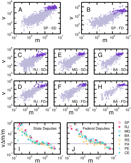
Figure 1: Scaling relation between number of votes and money spent. The light purple circles show the relation between the number of votes and the declared campaign expenditure of each candidate in the state (SD) and federal deputies (FD) elections in 2014 for the four largest states in Brazil: São Paulo (A, B), Rio de Janeiro (C, D), Minas Gerais (E, F), and Bahia (G, H). Despite the large fluctuations, there is an unambiguous correlation between votes and money. In each panel, the data for elected candidates are highlighted in dark purple circles. In order to see the nuances of the correlation, we plotted in a normalized relation for (I) state and (J) federal deputies for the eight largest states in Brazil. The symbols represent the normalized ratio $\langle v\rangle\Delta m/m$, where we first calculate the average number of votes in log-spaced bins along $m$. If we assume a linear correlation, the multiplicative constant is $\Delta m=M/n$. The normalization provides us a direct observation of the nonlinearity in the dependence of votes on money. We see a global sublinear behavior, where the wealthier candidates display a lower fraction of votes per money.

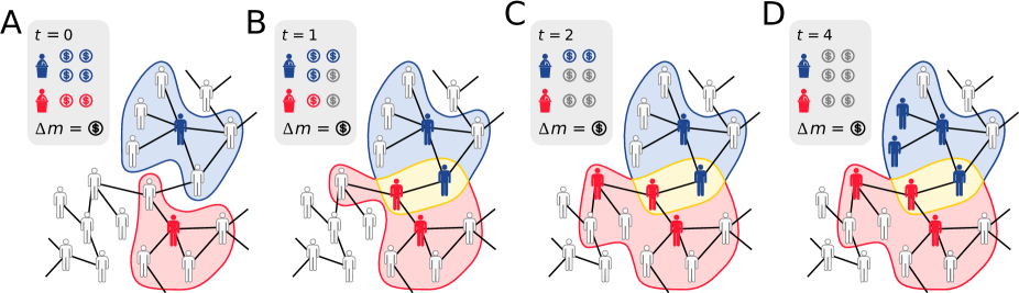
Figure 2: Model’s pictorial sketch. Here, two candidates compete for votes in a social network with undecided (light gray) individuals. (A) The blue candidate has initially a budget of 4 (four) monetary units, while the campaign for the red candidate has a budget of 2 (two) monetary units. In this example, both candidates also has one decided voter at the beginning of the process, namely, the blue voter at the top part of the network and the red one at the bottom part of the network. The highlighted regions enclose the initial voter each campaign has and the acquaintances of each initial voter. These regions represent operational areas the campaigns will act at the next time step in order to convince undecided voters to vote for their associated candidates. (B) One undecided voter inside each operational area is randomly chosen, becoming then decided voters. Accordingly, each budget campaign decreases by the amount of $\Delta m=\$$. As a consequence of new decided voters, the operational areas grow, and since two acquaintances become voters of different candidates, the operational areas of the campaigns now overlap. This region where both campaigns can act is represented in yellow. (C) While the red candidate’s campaign chose an undecided voter, increasing its operational area, blue campaign ineffectively spends money on a decided voter. (D) At the end of the campaign process, when all campaigns run out of funds, the campaign with larger initial budget ends the process with more adopters, but his/her campaign is less efficient, resulting in a diseconomy of scale.

We start by assembling the data sets on the entire electoral outcome and campaign expenditure of candidates from all 26 Brazilian states. Figure 1 displays the number of votes $v$ versus the declared campaign expenditure $m$ of each candidate for the top 4 Brazilian states in terms of population, namely, São Paulo (Figs. 1A and 1B), Rio de Janeiro (Figs. 1C and 1D), Minas Gerais (Figs. 1E and 1F) and Bahia (Figs. 1G and 1H). As depicted in Fig. 1, the clouds of points are neatly correlated and follow a clear trend. This trend is observed in all representative elections for all Brazilian states (see Supporting Information Section I).

To extract the main relationship between $v$ and $m$, we average the number of votes in log-spaced bins along $m$, which provides an estimation for the empirical relation of $\langle v\rangle$ as a function of $m$. In order to plot results for different states in the same figure, we perform a scale transformation on $\langle v\rangle$ by supposing simple linear relation $\langle v\rangle=c\times m$, where $c$ is a characteristic constant of a given election. If we define the average price of a vote as $\Delta m=\sum_{i}m_{i}/\sum_{i}v_{i}$ and suppose that it is roughly uniform across candidates, it is easy to see that $c=1/\Delta m$. Here, $v_{i}$ is the number of votes of candidates $i$. If the relation between votes and money is linear, then the plot of $\langle v\rangle\times(\Delta m/m)$ should be a constant function of $m$ with value close to $1.0$.

In Figs. 1I and 1J, we plot $\langle v\rangle\Delta m/m$ as a function of $m$ for the state legislative assembly and federal congress elections, respectively, for the year of 2014 and for the eight most populated states in Brazil. The result shows a consistent nontrivial dependence of votes on money spent in campaign. For small values of $m$, we observe a rapidly decrease of $\langle v\rangle\Delta m/m$. For intermediate expenditures in the range R$10,000 $<m<$ R$100,000, we observe an apparent linear dependence of $v$ with respect to $m$. Finally, for $m>$ R$100,000, a noticeable departure from linearity is observed, that is, wealthier candidates need a disproportionately large amount of money to obtain a single vote as compared with less successful candidates within the same range of financial resources.

A general model for the price of a vote
Here, we propose a general model for the price of a vote. We consider an electoral process composed of two separate groups of individuals, candidates and voters. All $s$ candidates can compete for the vote of all $n$ voters, and each candidate $i$ has a limited amount of money $m_{i}$ to spend on their campaigns. Thus, if at a given time $m_{i}=0$, the candidate becomes unable to compete for voters anymore. Here we assume that candidates can only conquer a single vote at a given time step and that voters, once they reach a decision, cannot change their minds anymore. As compared to the case of plurality elections, the last assumption is readily justifiable for proportional elections since, in this case, candidates do not compete directly for the same seat. As a consequence, voters do not feel compelled to rethink their decisions. In this way, because it is not possible to know if a voter reached a decision or not, campaigns can spend money on already decided voters, leading to ineffective use of financial resources.

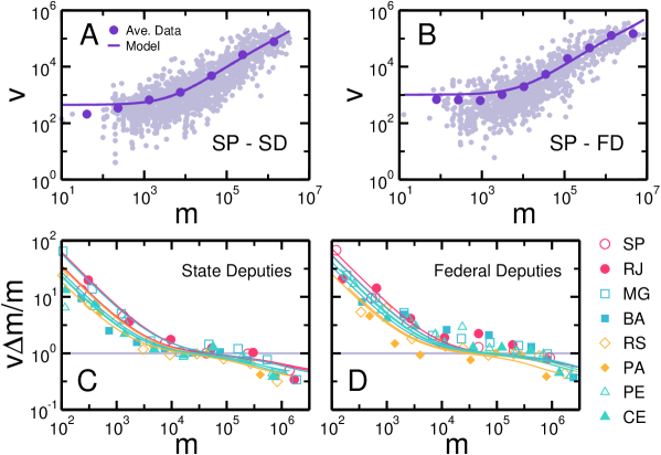
Figure 3: Modelling the nonlinear scaling. In order to verify if our model correctly fits the data, we show in (A) and (B) the São Paulo election for state and federal deputies in 2014, respectively. Each light purple circle corresponds to one candidate and the dark purples circles are the average number of votes in log-spaced bins along $m$. We see that our model shows a good agreement with the average behavior for all the money spectrum. In (C) and (D) we perform the same normalization process as in Fig. 2 but now with $\Delta m$ is estimated using Eq. 3. Each solid line shows the solution of our model. Despite its simplicity, our model features all nonlinear regimes seen in the data, which corroborates our theory that the inefficiency of wealthier candidates are mainly due to competition.

A pictorial description of the model is presented in Fig. 2. On a social network with undecided voters, represented by light gray individuals, two candidates start their campaigns with an initial amount of money $m$ and one single decided voter. This initial seed is represented in Fig. 2A by the blue and red individuals. The regions highlighted in blue and red represent the operational areas of the campaigns, enclosing the group of voters to whom the campaigns will spend money in order to turn undecided voters into decided voters. As depicted in Fig. 2B, at each time step each campaign chooses one voter inside its operational areas. If the chosen individual is an undecided voter, she/he becomes a decided voter. Accordingly, the overall campaign money is decreased by an amount of $\Delta m$. If the chosen voter is already a decided voter, as depicted in Fig. 2C, the campaign budget is also decreased by $\Delta m$, but the voter’s decision remains unchanged. We repeat this procedure until all campaigns run out of funds. In Fig 2D, we show a typical example of a competition for votes between two candidates during the electoral process described by our model. Although the candidate with the larger initial budget receives more votes at the end of the election, due to ineffective spending, the campaign of the poorer candidate is, in fact, more efficient.

In order to represent the reach of the traditional and social medias, as a first approximation, we apply this model on a complete graph, so that the time evolution of the number of votes of a given candidate $i$ can be written as

$$\frac{dv_{i}}{dt}=\left(1-\frac{S(t)}{n}\right)[m_{i}(t)>0],$$ (1)

where $S(t)=\sum_{i=0}^{s}v_{i}$ is the total number of decided voters at time $t$, and $\left[m_{i}(t)>0\right]$ is the Iverson bracket, which is $1$ if the condition inside the brackets is satisfied, and $0$ otherwise. The right-hand side of the Eq. 1 is the probability of candidate $i$ to choose an undecided voter at time $t$. Equation 1 explicitly requires a definition for the rate of money expenditure, $dm_{i}/dt$, which determines the gradual decrease in financial resources of candidate $i$. As simplifying assumptions, we consider that the amount of money spent during the campaign decreases linearly, $dm_{i}/dt=-\Delta m_{i}$, and that this constant rate is the same for all candidates, $\Delta m_{i}=\Delta m$, $\forall i$.

The probabilistic feature of Eq. 1 is central to confirm our hypothesis that electoral outcome is an output of campaign expenditure due to a competition process. This is shown here by first considering the case without competition, where $s\ll n$. Also, we assume that $n\Delta m\gg m_{i}$ for all $i$, so that the candidate with the highest amount of funds do not have enough money to reach out the whole network. By doing so, it is unlikely that the extent of the candidates’ campaigns overlap, and therefore, a candidate would not waste her/his campaign money on a decided voter of another candidate. As a consequence, since the probability of candidate $i$ to conquer an undecided voter is not affected by another campaign, $S(t)$ can be replaced by $v_{i}$ in Eq. 1, leading to an uncoupled system of differential equations, whose solution is given by,

$$v_{i}=n-(n-v_{0,i})e^{-m_{i}/n\Delta m},$$ (2)

where $v_{0,i}$ is the initial number of votes of candidate $i$. Since $n\Delta m\gg m_{i}$, and assuming that $(n-v_{0,i})\approx n$, by expanding the exponential and taking its first order approximation, we can write the number of votes as $v_{i}\approx v_{0,i}+m_{i}/\Delta m$ . As we discuss next, this simple model do not suffice to explain the whole complexity of the relation between $v$ and $m$. The first two regimes presented in Fig. 2 can be understood in therms of this approximation. For the regime of low $m$, where the experimental data do not exhibit a clear correlation, the candidates start the race with $v_{0,i}$ votes. Since they cannot afford a long run and/or a large expenditure, their final performance fluctuates around the initial value $v_{0,i}$, which depends on different factors, such as free volunteer engagement. As campaign money increases, the linear part overcomes the initial number $v_{0,i}$, and a linear regime emerges. However, in the scenario without competition, the linear behavior remains at large $m$.

We now consider the competition between candidates as a possible cause for the transition from linear to sublinear regime. Disregarding all previous simplifying assumptions and integrating Eq. 1, we find

$$v_{i}=v_{0,i}+\frac{m_{i}}{\Delta m}-\frac{1}{n\Delta m}\int_{0}^{m_{i}}S(m^{\prime})dm^{\prime},$$ (3)

where the integration of the Iverson bracket over time gives the total time candidate $i$ has to perform her/his campaign, $m_{i}/\Delta m$, and we used $dm^{\prime}/dt^{\prime}=-\Delta m$ to change the variable of integration on the last term.

It is possible to find a differential equation for $S(m^{\prime})$ by taking Eq. 1 and summing over $i$. After solving it for $S(m^{\prime})$ and integrating the last term of Eq. 3 (see Supporting Information Section II for details of the analytical solution), we find a set of nonlinear coupled equations that must be solved, candidate by candidate, following an increasing order of $m_{i}$ values. As a consequence, the number of votes of candidate $i$ depends on the whole distribution $P(m)$ through the integral term in Eq. 3.

Equation 3 has a simple interpretation. As in the case without competition, all candidates begin their run with an initial number of votes, and those with sufficient money to keep running enter in a linear regime controlled by the rate $\Delta m/m$. Nonetheless, as we will see next, candidates with sufficient campaign funds may start to waste their money on decided voters, a behavior that is substantiated by the presence of $S(m^{\prime})$ in the last term of Eq. 3, which encloses the competition dynamics. We consider this collective influence of the total financial resources from all candidates during the campaign as an important result, since it provides a bridge between campaign expenditure and electoral outcome, which is the basis of the remaining results that follows.

In order to obtain a solution for the model, we use as inputs the money $m_{i}$ of each candidate $i$, obtained from data, the total number of voters $n$, an initial number of votes $v_{0}$, and an estimated value for $\Delta m$. For all candidates, we define $v_{0}$ as the average number of votes of candidates with less then R$1,000. The parameter $\Delta m$ is calculated as a function of the turnout rate $T=S_{f}/n$, where $S_{f}=\lim_{t\to\infty}S(t)$ is the total number of votes at steady state. We can therefore write the final fraction of votes as

$$T=1-e^{-M/(n\Delta m)},$$ (4)

where $M=\sum_{i}m_{i}$ is the total amount of money in the campaign process. Therefore, we estimate $\Delta m$ using Eq. 4 such that the total number of votes fits the turnout election data.

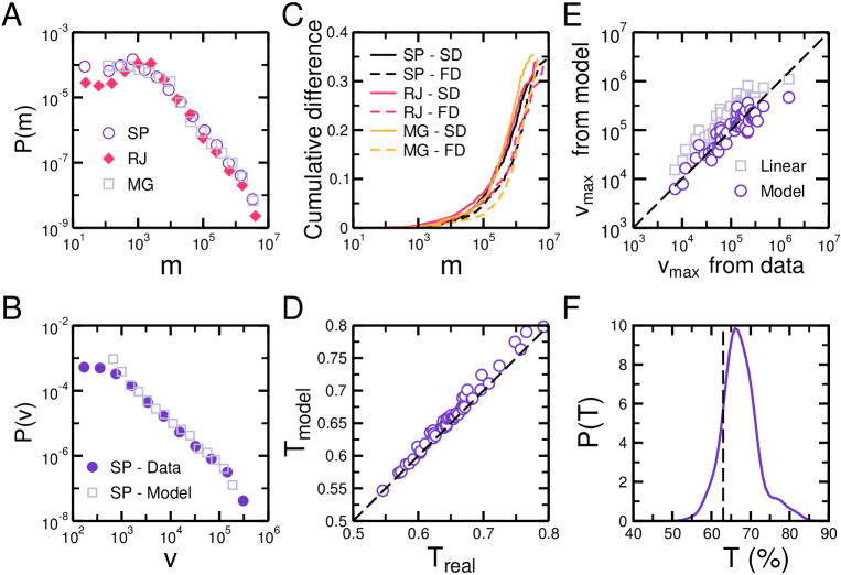
Figure 4: Analytical results of the model. In order to derive the distribution of votes, our model takes as input the distribution of money. (A) We see that the distributions of money for the state deputies in São Paulo (SP), Rio de Janeiro (RJ) and Minas Gerais (MG) reveal long tails characteristic. (B) We can now compare the actual distribution (circles) of votes, $P(v)$, with the ones obtained by our model (squares) for the election of state representatives in São Paulo. Clearly, we can see that our model have a good agreement with the data showing that the universal long tail characteristic of $P(v)$ is a direct consequence of the money as an input for dynamical competition process. (C) Relative difference between the cumulative distributions of the predictions for the model with and without competition. Here we show the results for the elections of state deputies (SD) and federal deputies (FD) for São Paulo (SP), Rio de Janeiro (RJ) and Minas Gerais (MG). No noticeable difference between both approaches can be observed for the region of $m<{\rm R}\$10,000$. However, for the region of top spenders candidates ($m>{\rm R}\$1,000,00$), those who get elected, the relative difference is drastic, varying from $30\%$ to $40\%$. (D) By solving our model, as expressed in Eq. 1, we calculate the expected number of votes that each candidate should have for an election. The total number of votes of that election divided by the number of voters $n$ is defined as the turnout ratio $T$. For all 56 parliamentary elections in 2014, we compared our estimation of the turnout ratio, $T_{\rm model}$, and the data ratio $T_{\rm data}$. The dashed line represents what would be the perfect agreement, $T_{\rm real}=T_{\rm model}$. As can be seen, the simulations (circles) exhibit a good agreement with the data. (E) We can also pick up the candidate with the largest number of votes $v_{\max}$ and see how our model estimates this value. As depicted, we see that the competition model (circles) better estimates $v_{\rm max}$ when compared with the linear model (squares), which always overestimates it. The non-parametric histogram of $T$ shown in (F) for the election of 2006, 2010, and 2014 reveals an average turnout value of approximately 67  which is consistent with our heuristic estimation of $T=1-e^{-1}\approx 63\%$ (vertical dashed line).

The results of the election in São Paulo state for state and federal deputies in 2014 are shown in Figs. 3A and 3B, respectively. As depicted, the predictions of our model (solid line) are in good agreement with the average values of the number of votes for different classes of candidates in terms of fund raising. Note that no fitting parameters are necessary for this comparison. For $m<$ R$1,000, our model exhibits a constant behavior, capturing the uncorrelated nature of the data. Additionally, for $m>$ R$1,000, an evident correlation between votes and money is present. This is better visualized when we plot in Figs. 3C and 3D the normalized ratio $\langle v\rangle\Delta m/m$ for the eight most populated Brazilian states. Here, the symbols represent the data average and the lines show the solution of our model for each state identified by color. For small and large values of $m$, we see that our model exhibits a clear deviation from a linear behavior. In other words, besides exhibiting this deviation for $m<$ R$1,000, a clear sublinearity is present for $m>$ R$100,000. Under the perspective of our model, the observed diseconomy of scale is a direct consequence of the competition among candidates (see Supporting Information Section III for a statistical comparison between our model with competition and the linear model without competition).

Social networks are known to display the small-world phenomenon, where the typical network distance between two individuals, $\ell$, is rather small when compared to the system size, $\ell\sim\log N$ Milgram67 ; Barabasi2016 . Our analytical solution on a complete graph works as a first approximation of such complex social network structure. In order to compare our model with a more realistic one, we apply the dynamics presented on Fig. 2 on a random graph Barabasi2016 (see Supporting Information Section IV). We found a good agreement between the solution on a complete graph model and the numerical simulation results obtained with a random graph model.

Frequency distribution of votes
One of the first empirical investigations concerning Brazilian elections was carried out to determine the distribution $P(v)$ of the number of candidates receiving $v$ votes Costa99 ; Costa2003 ; Moreira06 ; Loreto09 . Since then, several other studies have been devoted to elucidate the origin of the anomalous behaviors of $P(v)$ for other countries as well as to propose mathematical models that can provide some insight on the social and political mechanisms responsible for this statistical behavior Moreira06 ; Calvao2015 ; Fortunato2007 . In our modeling approach, however, the distribution of votes emerges as a natural outcome of the distribution of financial resources $P(m)$. As shown in Fig. 4A, the distribution $P(m)$ calculated for state deputies of three different states in Brazil can all be described in terms of a power-law type of decay extending over a region of approximately six orders of magnitude. Using those distributions as inputs, we determine $P(v)$ for each one of those elections. In Fig. 4B we compare the empirical votes distribution for the state of São Paulo with the one obtained by our model, which reproduces correctly the empirical distribution of votes among candidates, $P(v)$, for over two orders of magnitude (see Supporting Information Sec. V for results concerning the states of Rio de Janeiro and Minas Gerais). This implies that the observed non-Gaussian long tail form has its origin in the heterogeneous aspect of the distribution of campaign resources, regardless of the intricate social network and information dynamics behind the electoral process.

Model validation
To highlight the effect of the sublinearity on forecasting an election, we compute the relative difference between the cumulative vote distribution predicted by the linear model without competition and the one predicted by the model with competition. As shown in Fig. 4C, for state congress election in the top three populated Brazilian states, namely, São Paulo, Rio de Janeiro, and Minas Gerais, no significant difference is noticed between the two predictions for campaigns of low expenditure. However, for electoral campaigns that invested more than ${\rm R\$}10,000$, a substantial discrepancy between predictions can be noticed. For this region of top spenders, the cumulative difference can be drastic, going above $30\%$ in some cases.

We confirm the validity of our model by comparison with data from the 2014 state and federal deputy elections that took place simultaneously in the 26 states of Brazil. As shown in Fig. 4D, where each point corresponds to an election in a given state, the model results for the turnout rate $T$, as provided by Eq. 4, are compatible with the observed data. This agreement only confirms the self-consistency of our approach, since Eq. 3 has been used to estimate the parameter $\Delta m$. The predictive capability of the model can be effectively tested by comparing its estimate with real data for the largest number of votes obtained by a candidate in each election, $v_{max}$. As shown in Fig. 4E, while the results of our model (circles) gather around the identity line, demonstrating good quantitative agreement with real data, the linear approximation model, $v_{max}\approx v_{0}+m_{max}/\Delta m$ (squares), clearly overestimates the values of $v_{max}$.

At this point, we show that our theoretical framework allows for a forecast of the turnout ratio $T$, if the following assumptions are considered: (i) the candidates have knowledge of the total amount of resources $M$ during the campaign, and (ii) $\Delta m=M/n$, which corresponds to the most simple and equitable division of votes. As matter of fact, this last point is equivalent to assume that a complete turnout can be achieved, namely, $T=100\%$, as in the case without competition. In other words, the candidates devise their strategy presupposing that they will obtain the maximum possible number of votes, therefore disregarding the competition among them. This heuristic argument leads to a fraction of valid votes, $T=1-e^{-1}\approx 0.63$. As shown in Fig. 4F, the histogram of the number of total valid votes for all Congress elections in the years 2006, 2010 and 2014 indicates an average turnout value of 0.67, which is in close agreement with our model prediction. Finally, we also tested our theoretical approach by applying the principle of maximum entropy Jaynes1957 and found that the statistical dispersion of the model is consistent with real data from elections (see Supporting Information Sec. VI).

Discussion

As a result of the competition between candidates in real elections, the nonlinear relation between $v$ and $m$ obtained here can complement other statistical analyses for political campaign and electoral outcome Klimek2012 ; Borghesi2010 ; Nuno2010 ; Borghesi2012 . These analyses enable the detection of a number of statistical patterns of electoral processes, such as the relations between party size and temporal correlations Andresen2008 , the relations between the number of candidates and voters Mantovani2011 , and the distribution of votes Costa99 ; Calvao2015 ; Fortunato2007 ; Fortunato2013 . Our approach goes beyond the examination of statistical patterns by providing a theoretical framework that clarifies a number of key issues on the economical features of electoral campaigns. First, we proposed a simple modeling framework, whose analytical solution is statistically consistent with extensive data relating financial resources of political and electoral outcomes. Interestingly, the same model also provides estimates for the distribution of votes among candidates and the electorate turnout rate that are in good agreement with real data.

A close inspection of the campaign data investigated here reveals a ubiquitous nontrivial relation between $v$ and $m$ for all elections investigated. More precisely, we observed that this relation is an unambiguous sublinear correlation between the money spent by candidate and her/his number of votes $v$, specially for the top spender candidates, indicating that the electoral process works in a state of diseconomy of scale. To explain this behavior in the campaign economy, we propose a general model for marketing where candidates compete with each other and must spend their money in order to get votes. Despite its simplicity, the model proves capable of reproducing the complexity of the dependence of $v$ with respect of $m$. This good agreement makes our model a possible alternative to study other aspects of human collective behavior involving, for example, diffusion of innovation and decision-making, such as the competition in market share where companies invest in advertising for products.

Acknowledgements
We thank the Brazilian agencies CNPq, CAPES, FUNCAP, and the National Institute of Science and Technology for Complex Systems (INCT-SC) in Brazil for financial support, and the support by Army Research Laboratory Cooperative Agreement Number W911NF-09-2-0053 (the ARL Network Science CTA) in the US.

Author contributions
All authors contributed to all parts of the study.

Additional information
Supplementary information accompanies this manuscript.

Competing interests
The authors declare no competing interests.

Supplementary Information: The price of a vote: diseconomy in proportional elections

I The Data

I.1 Data Description

In the main text we investigate the effect of the investment of candidates on campaign thanks to the available data containing the total donation received by and the expenses of each candidate. We analyze Brazilian elections for two different kinds of legislators, more specifically, the federal and state deputies. Their function is to legislate in the unicameral system of each Brazilian state. The federal deputies are representatives in the chamber of deputies of the national Congress. They are also elected for a four year term by a proportional system. The number of elected federal deputies is proportional to the population of each one of the 26 states. The data is available at the website of the Brazilian Federal Electoral Court S_TSE . By force of law, each candidate must provide a detailed description of his/her campaign expenditure with specific informations such as the value, date and type of expense. All this information can be accessed by the public, however in order to know the total cost of the campaign and the number of votes of each candidate, it is necessary to process the database computationally. In Tables 1 and 2, we show a detailed description of the data for each state. State deputies are local representatives elected for a four year term by a proportional system.

I.2 Results for all States

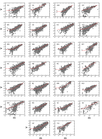
Figure S1: Modeling the nonlinear scaling for state deputies in all federal states. We show how the model fits the data of state deputies election for all states in alphabetic order (AC: Acre, AL: Alagoas, AM: Amazonas, AP: Amapá, BA: Bahia, CE: Ceará, ES: Espírito Santo, GO: Goiás, MA: Maranhão, MG: Minas Gerais, MS: Mato Grosso do Sul, MT: Mato Grosso, PA: Pará, PB: Paraíba, PE: Pernambuco, PI: Piauí, PR: Paraná, RJ: Rio de Janeiro, RN: Rio Grande do Norte, RO: Rondônia, RR: Roraima:, RS: Rio Grande do Sul, SC: Santa Catarina, SE: Sergipe, SP: São Paulo, TO: Tocantis). Each gray circle represents the data for one candidate and the red line is the result of the analytical model. We see that the model shows a good agreement with the average behavior for all states.

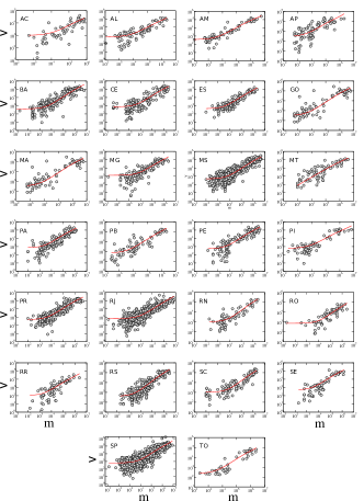
Figure S2: Modeling the nonlinear scaling for federal deputies in all federal states. We show how the model fits the data of federal deputies election for all states in alphabetic order (AC: Acre, AL: Alagoas, AM: Amazonas, AP: Amapá, BA: Bahia, CE: Ceará, ES: Espírito Santo, GO: Goiás, MA: Maranhão, MG: Minas Gerais, MS: Mato Grosso do Sul, MT: Mato Grosso, PA: Pará, PB: Paraíba, PE: Pernambuco, PI: Piauí, PR: Paraná, RJ: Rio de Janeiro, RN: Rio Grande do Norte, RO: Rondônia, RR: Roraima:, RS: Rio Grande do Sul, SC: Santa Catarina, SE: Sergipe, SP: São Paulo, TO: Tocantis). Each gray circle represents the data for one candidate and the red line is the result of the analytical model. We see that the model shows a good agreement with the average behavior for all states.

Here we summarize the results of our model for the election in 2014 of state and federal deputies in each Brazilian state. Figure S1 shows the data obtained for state deputies election and Fig. S2 shows data for the federal deputies election.

II Analytical Solution

II.1 Calculation of the expected turnout rate $T$

Following from Eq. (1) in the main text and summing over $i$, we can find a differential equation for the decided number of voters $S$, which reads

$$\frac{dS}{dt}=\left(1-\frac{S(t)}{n}\right)r(t),$$ (S1)

where $n$ is the total number of voters, and $r(t)=\sum_{i}[m_{i}(t)>0]$ is the number of candidates who still have money at instant $t$, which depends solely on the distribution of money. After integrating Eq. (S1), we find that

$$S(t)=n-(n-S(0))\exp\left(-\frac{1}{n}\int_{0}^{t}r(t^{\prime})dt^{\prime}\right).$$ (S2)

This equation enables us to compute the expected turnout rate $T$ of the election as a function of the average price of a vote $\Delta m$, the total money $M$, and $n$. To compute $T$, it is necessary to take the limit $t\to\infty$, first. At this limit, we are able to compute the value where $S$ saturates. Then, we can define $T$ as

$$T=\frac{1}{n}\lim_{t\to\infty}S(t).$$ (S3)

In order to compute the integral in Eq. (S2) at this limit, we recall from the main text that $dt=-dm/\Delta m$. Then, the integral becomes

$$\lim_{t\to\infty}\int_{0}^{t}r(t^{\prime})dt^{\prime}=\int_{0}^{\infty}\sum_{i=0}^{N_{c}}[m_{i}(m^{\prime})>0]dm^{\prime}/\Delta m,$$ (S4)

where $N_{c}$ is the total number of candidates. After commutating the summation with the integral, and integrating the Iverson’s bracket over $m^{\prime}$, we find that

$$\lim_{t\to\infty}\int_{0}^{t}r(t^{\prime})dt^{\prime}=\frac{M}{\Delta m},$$ (S5)

which leads to

$$T=1-e^{-M/(n\Delta m)}.$$ (S6)

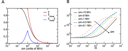
Figure S4: Dependence with $\Delta m$. The solution of the mean field model enables us to calculate the turnout radio $T$ as a function of the dimensionless $n\Delta m/M$ parameter. In (A) we compare the turnout for the linear case where we excluded the competition between the candidates, $T_{linear}$, with the case with competition, $T$. The competition creates an exponential saturation, which increases the waste of money when candidates seek new voters. By looking at the difference $T_{linear}-T$, we can see that this inefficiency is maximum when $n\Delta m/M=1.0$. In (B) we show that as we decrease $\Delta m$ the values of $v(m)$ usually increases, as expected by the definition of $\Delta m$. However, there is a point where a saturation appears as the total number of votes starts to get close to the size of the system, resulting on a diseconomy of scale due to the competition between candidates.

Figure S4A shows the turnout rate $T$ as a function of $\Delta m$ computed from Eq. (S6) for the model with competition, and for the model without competition ($T_{\rm linear}$). The number of votes (or money) lost by  competition can be evaluated by looking at the difference between $T$ and $T_{\rm linear}$. We see that there is a maximum loss when $\Delta m=M/n$.

II.2 Calculation of the expected number of votes $v$

By integrating Eq. (1) from the main text and performing a change of variables, we find that $v_{i}$ can be written as a function of $m_{i}$ as

$$v_{i}=v_{i}(0)+\frac{m_{i}}{\Delta m}-\frac{1}{\Delta m}\int_{0}^{m_{i}}\frac{S(m^{\prime})}{n}dm^{\prime}.$$ (S7)

Using Eq. (S2), we can rewrite the above equation as

$$v_{i}=v_{i}(0)+\frac{1}{\Delta m}\left(1-\frac{S(0)}{n}\right)\int_{0}^{m_{i}}\exp\left[-\frac{1}{n\Delta m}\int_{0}^{m^{\prime}}r(m^{\prime\prime})dm^{\prime\prime}\right]dm^{\prime}.$$ (S8)

To find an analytical expression for $v$, we first decompose the external integral as

$$\begin{split}v_{i}&=v_{i}(0)+\frac{1}{\Delta m}\left(1-\frac{S(0)}{n}\right)\int_{0}^{m_{i-1}}\exp\left[-\frac{1}{n\Delta m}\int_{0}^{m^{\prime}}r(m^{\prime\prime})dm^{\prime\prime}\right]dm^{\prime}\\ &+\frac{1}{\Delta m}\left(1-\frac{S(0)}{n}\right)\int_{m_{i-1}}^{m_{i}}\exp\left[-\frac{1}{n\Delta m}\int_{0}^{m^{\prime}}r(m^{\prime\prime})dm^{\prime\prime}\right]dm^{\prime},\\ \end{split}$$ (S9)

that compared with Eq. (S8) can be rewritten as

$$\begin{split}&v_{i}=v_{i}(0)-v_{i-1}(0)+v_{i-1}\\ &+\frac{1}{\Delta m}\left(1-\frac{S(0)}{n}\right)\int_{m_{i-1}}^{m_{i}}\exp\left[-\frac{1}{n\Delta m}\int_{0}^{m^{\prime}}r(m^{\prime\prime})dm^{\prime\prime}\right]dm^{\prime}.\\ \end{split}$$ (S10)

The result of this integral relies on the limits of the external integral. Using the definition of $r(m)$ for the external interval $m^{\prime}\in[m_{i-1},m_{i}]$, we find that

$$\int_{0}^{m^{\prime}}r(m^{\prime\prime})dm^{\prime\prime}=m_{0}+m_{1}+m_{2}+...+m_{i-1}+(N_{c}-i)m^{\prime}.$$ (S11)

By solving the integrals, we finally find that the number of votes $v_{i}$ is given by

$$\begin{split}&v_{i}=v_{i}(0)-v_{i-1}(0)+v_{i-1}\\ &-\frac{n-S(0)}{N_{c}-i}e^{-\sum_{j=0}^{i-1}m_{j}/(n\Delta m)}\left[e^{-\frac{(N_{c}-i)m_{i}}{n\Delta m}}-e^{-\frac{(N_{c}-i)m_{i-1}}{n\Delta m}}\right].\end{split}$$ (S12)

As we can see from Eq. (S12), the number of votes $v_{i}$ of a candidate $i$ is not only a function of his budget $m_{i}$, but also depends on the whole distribution $P(m)$. In Fig. S4B we show how $v(m)$ changes with $\Delta m$. As $\Delta m$ decreases, a large fraction of the voters become decided (i.e., $T\to 1$), and $v(m)$ displays a saturation for larges values of $m$ resulting on the diseconomy of scale due to the competition between candidates.

III Statistical comparison of models

In order to compare our model with the simple case without competition, we make use of the Akaike’s Information Criterion (AIC) S_Motulsky2004 . The AIC is a model selection method that uses information theory to compare the relative estimation of the information lost by mathematical models used to generate data. Here, we used AIC to measure the relative quality of our model when compared with the linear non-competitive model. Suppose that we have a model with $P$ parameters that fits a data set with $N$ points. Then, the AIC is defined as

$$AIC=N\ln\left(\frac{RSS}{N}\right)+2(P+1),$$ (S13)

where RSS is the residual sum of squares given by

$$RSS=\sum_{i=1}^{N}(x_{i}-X_{i})^{2}.$$ (S14)

Here, $x_{i}$ is the $i^{\rm th}$ value of the variable to be predicted and the $X_{i}$ is the predicted value of $x_{i}$. We calculate the AIC for each model using Eq. (S13). Then, by Akaike’s criterion, the preferred model is the one with the minimum AIC value. Here, we label the model without competition as WOC and the more complex model, where there is competition, as WC. The difference in AIC is then defined as $\Delta AIC=AIC_{\rm WC}-AIC_{\rm WOC}$. Once this difference is computed we calculate the probability that model WC minimize the information loss:

$$P_{\rm WC}=\frac{e^{-0.5\Delta AIC}}{1-e^{-0.5\Delta AIC}}.$$ (S15)

Therefore, the probability that model WOC minimizes the information loss is $P_{\rm WOC}=1-P_{\rm WC}$. Here, we define the ratio between $P_{\rm WC}$ and $P_{\rm WOC}$ as the evidence ratio, which means how many times the model WC is more likely to minimize the information loss. We then performed this analysis for federal and state deputies for the 2014 elections in all 26 Brazilian states. The model WC and the model WOC are compared to the logarithm of the data (Tables 3 and 4), and to the data without applying the logarithm (Tables 5, and 6). The AIC shows that the model with competition best explains the data when compared to the linear model in all studied cases.

IV Simulation on a Complex Network

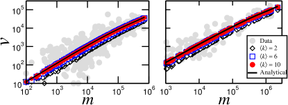
Figure S3: Simulation on a random network model. Here we compare the analytical solution (black line) with the simulation on a random Erdös–Rényi network for the 2014 Espírito Santo state election of federal deputies (A) and state deputies (B). Here, each gray circle represents the data for one candidate. We used three different values of average connectivity: $\langle k\rangle=2$ (black diamonds), $\langle k\rangle=6$ (blue squares) and $\langle k\rangle=10$ (red circles). Each symbol is the result of a logarithmic binning for the money ($m$) axis over the simulation. We see that as we increase the average network degree, the simulation presents better agreement with the analytical solution. However, the analytical solution seems to capture the overall behavior for all networks tested. The apparent disagreement for $\langle k\rangle=2$ is a consequence of a smaller effective size of the network, since an important fraction of nodes are not connected with the largest cluster.

In order to solve analytically the model, we make use of a mean field approximation where the network is a fully connected graph. To see if our solution still holds for a more complex topology, we performed simulations using the Erdös–Rényi network model with three different values for the average degree: $\langle k\rangle=2$, $6$ and $10$. As we can see in Fig. S3A and B, for federal and state deputies, respectively, we find a good agreement between the analytical solution (black line) and the real data (grey circles) for $\langle k\rangle=6$ and $10$. Due to computational performance, we chose the state of Espírito Santo to perform the simulations. First, we made use of the candidates’ budget for the 2014 election as an input for the distribution of money $P(m)$. The network size is taken from the number of registered voters in Espírito Santo, $N=2653536$, as presented in Table 1 and 2. Each candidate starts the simulation with only one node as a decided voter. This node is the initial seed for the candidate’s marketing campaing. The overall underestimation of the number of votes for $\langle k\rangle=2$ can be understood by noting that an important fraction of the network is made of unconnected nodes, therefore, for the candidates with seeds in the largest cluster the network seems to be smaller.

V Frequency distribution of votes

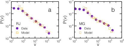
Figure S5: Comparison between the actual distribution of votes with the ones obtained by our model. Here, we show the comparison for the states of (a) Rio de Janeiro and (b) Minas Gerais. Again, the good agreement indicates that the long tail of $P(v)$ is a direct consequence of the money as an input for the dynamical process.

Here, we show the comparison between the empirical votes distribution for the states of Rio de Janeiro (Fig. S5a) and Minas Gerais (Fig. S5B) with the one obtained by our model. Again, the model reproduces correctly the empirical distribution of votes among candidates, $P(v)$.

VI Study of the dispersion

Our model allow us to calculate the mean or expected value of the number of votes. However, to fully describe the election we have also to study the statistical dispersion, which is given by the conditional probability distribution $p(v|m)$. We can use the concept of maximum entropy probability distribution (MaxEnt) from information theory to guess which is the $p(v|m)$ that maximizes the Shannon’s Entropy S_Jaynes1957 . Imposing only a constraint for the mean $\langle v\rangle$, the maximum entropy continuous distribution is exponential,

$$p(v|m)=\frac{1}{\langle v\rangle}e^{-\frac{v}{\langle v\rangle}},$$ (S16)

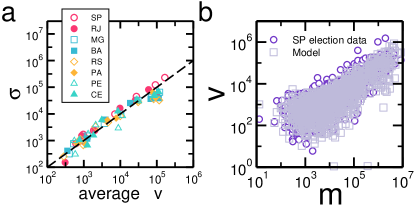
Figure S6: Test of statistical dispersion. It is widely known that the exponential distribution have the property that its mean and standard deviation are equal. Therefore we use this property in order to test if the dispersion along the mean follows an exponential distribution, as predicted by the MaxEnt hypothesis. In (a) we see that for state deputies of the eight largest states in 2014 election the data is in close agreement with $\sigma=\langle v\rangle$ (dashed line). (b) of votes calculate by our model to generate a random election. Here we show for the state of São Paulo that when we add random noise to our model (squares), we obtain a cloud that closely resembles the actual data (circles).

which has the property that the mean and standard deviation are the same. We see in Figure S6A that our data show a close linear relationship with approximately unit slope $\sigma\approx\langle v\rangle$, which strongly indicates that the Eq. (S16) accounts for all the random variation on $v(m)$ with the expected value calculated by our model. In the inset of Fig. 4F from the main text, we show these two elements in a simulation for the election of state deputy for the state of São Paulo, the greatest electoral college in Brazil. Figure S6B shows that the addition of random dispersion to our model leads to a remarkable resemblance with real election data.

		Federal deputies
State	n	M (R$)	$S_{f}$	$T$ (%)	r–pearson	p–value
AC	506724	8480357.97	368332	72.6888799425	0.722748043319	3.30192976139e-11
AL	1995727	18421969.9	1283120	64.2933627696	0.840392141284	4.92302048603e-31
AM	2226891	23414726.56	1560085	70.0566395032	0.905459637663	9.23656309525e-31
AP	455514	8484530.19	368061	80.8012486993	0.566853357973	1.31431785604e-10
BA	10185417	72471496.94	5982371	58.7346693807	0.698084305668	2.28399775277e-49
CE	6271554	34838910.83	4002492	63.819780552	0.737909089987	7.95861881821e-36
ES	2653536	19490814.39	1665277	62.7569024879	0.822155443552	1.7418221573e-41
GO	4331733	65145051.12	2824329	65.2009022717	0.66788295422	6.05466767683e-20
MA	4497336	21197635.67	2836788	63.0770749617	0.685587130132	8.36126780457e-35
MG	15248681	160498695.1	9273472	60.8149124505	0.806652645383	1.27631105412e-147
MS	1818937	29384486.15	1174221	64.5553419387	0.778880439738	1.8509184753e-25
MT	2189703	27179850.24	1334861	60.9608243675	0.86687644675	1.61425424251e-33
PA	5188450	19219663.68	3496764	67.3951565496	0.714596611048	4.68308734801e-30
PB	2835882	14092397.88	1773112	62.5241811895	0.855261326688	2.61029697443e-30
PE	6356307	51507676.68	4129147	64.9614154886	0.728324391535	1.46267253887e-27
PI	2345694	24898627.07	1587477	67.6762186372	0.656433873665	1.22040618126e-13
PR	7865950	69592048.16	5275880	67.0723815941	0.728660777076	6.64008626188e-52
RJ	12141145	110784215.29	7063961	58.1820001326	0.56473987424	2.1291171572e-85
RN	2327451	14178893.28	1451341	62.3575319094	0.882530044098	1.40216619215e-30
RO	1127154	16967025.91	740924	65.7340523123	0.683327785935	7.96683605323e-13
RR	299558	8358613.48	225631	75.3213067252	0.598924952323	3.49851465097e-09
RS	8392033	57254432.25	5501353	65.554472915	0.836559267138	4.74667303986e-84
SC	4859324	31716424.53	3120297	64.2125736008	0.869812045153	2.11886214421e-41
SE	1454165	8057895.72	974311	67.0014063053	0.684912931565	2.44474497848e-12
TO	996887	15619685.1	670894	67.2989014803	0.76979251044	1.60978392322e-10
SP	31998432	241919492.64	19072393	59.6041487283	0.483246969693	9.81028340891e-81

Table 1: Data description for Federal deputies. Here we describe the main properties of the data for the federal deputies election from all Brazilian states. For each state we show the number of voters registered $n$, the total cost of the campaign in Brazilian Reais (R$) $M$, the number of valid votes $S_{f}$, and the turnout percentage $T$.

		State deputies
State	n	M (R$)	$S_{f}$	$T$ (%)	r–pearson	p–value
AC	506724	10656037.7	377299	74.4584823296	0.803577951964	1.59880493578e-114
AL	1995727	19627276.99	1314659	65.8736891368	0.836240190525	8.11032735735e-76
AM	2226891	28001756.68	1547128	69.4747969254	0.498718455137	4.12728400638e-39
AP	455514	5626676.58	373731	82.0459963909	0.647712202199	7.66012489633e-44
BA	10185417	47294333.36	6053428	59.432304048	0.782568469296	1.25445144149e-126
CE	6271554	32576249.09	4095292	65.2994776095	0.686934485759	7.21069456863e-83
ES	2653536	23289124.65	1748232	65.8831084259	0.741623876986	4.30172166816e-85
GO	4331733	79310623.34	2882804	66.550823885	0.734121134203	3.1534575998e-129
MA	4497336	25979148.94	2917772	64.8777854268	0.839414632196	1.67610556861e-134
MG	15248681	177676580.98	9283721	60.8821248212	0.224029765254	4.52706918339e-14
MS	1818937	45948066.57	1204007	66.1928917824	0.799004169269	6.08398880781e-90
MT	2189703	51639423.61	1375357	62.8102075944	0.771404926583	2.02454597864e-62
PA	5188450	31595425.94	3453031	66.5522651274	0.715064099361	1.78371156902e-110
PB	2835882	17219860.72	1835376	64.7197591437	0.782772014141	1.67491078919e-74
PE	6356307	40641680.29	4171737	65.6314586441	0.748176330675	1.36075786856e-90
PI	2345694	20320016.99	1607165	68.5155438007	0.816180285209	2.19894569952e-58
PR	7865950	61749634.55	5298846	67.3643488708	0.878519254427	1.18750225791e-247
RJ	12141145	130048101.34	7122375	58.6631244417	0.572037787678	5.93043422869e-167
RN	2327451	18343797.5	1529149	65.700588326	0.850127492405	3.79357570719e-72
RO	1127154	25138956.64	761590	67.5675196113	0.741913371628	3.21262552227e-70
RR	299558	13376926.76	242398	80.9185533352	0.813681589893	8.41908443078e-96
RS	8392033	54552702.15	5592657	66.6424571972	0.691245148201	3.6535374402e-98
SC	4859324	52245781.28	3280653	67.5125387811	0.816495812077	1.75144104038e-102
SE	1454165	8833829.91	967550	66.5364659444	0.716103939585	1.17133851209e-28
TO	996887	20185053.82	699008	70.1190806982	0.864802148991	1.46231152842e-78
SP	31998432	231516634.41	17618073	55.0591760246	0.722245302764	1.00059011444e-314

Table 2: Data description for State deputies. Here we describe the main properties of the data for the state deputies election from all Brazilian states. For each state we show the number of voters registered $n$, the total cost of the campaign in Brazilian Reais (R$) $M$, the number of valid votes $S_{f}$, and the turnout percentage $T$.

	Federal deputies
State	$\Delta$ AIC	Probability WOC	Probability WC	Evidence radio
AC	6.1827384262	0.0434646736	0.9565353264	22.0071898888
AL	4.7608349884	0.0846782011	0.9153217989	10.8094147898
AM	2.6647303199	0.2087684091	0.7912315909	3.7899967439
AP	2.806065353	0.1973353125	0.8026646875	4.0675167435
CE	10.5123485714	0.0051881611	0.9948118389	191.7465189
ES	14.4468382526	0.0007287731	0.9992712269	1371.1692559
GO	7.4677125018	0.0233425922	0.9766574078	41.8401435584
MA	7.7592626578	0.0202403068	0.9797596932	48.4063657539
MS	10.1109475602	0.0063339711	0.9936660289	156.878838813
MT	3.9037010608	0.1243517168	0.8756482832	7.0417064229
PA	9.663695483	0.0079087312	0.9920912688	125.442532017
PB	4.6657768971	0.0884355349	0.9115644651	10.3076717549
PI	2.3415470513	0.2367151943	0.7632848057	3.2244858966
RN	5.1455026334	0.0709128217	0.9290871783	13.1018221599
RO	9.807097669	0.0073655493	0.9926344507	134.767198525
RR	1.8879845033	0.2800946322	0.7199053678	2.5702219362
SC	13.3469679287	0.0012623917	0.9987376083	791.147136976
SE	2.8635043257	0.1928258238	0.8071741762	4.1860273715
TO	5.8040508651	0.0520535295	0.9479464705	18.2109931789
BA	16.0404485774	0.0003286382	0.9996713618	3041.85951117
MG	32.2756994687	9.80439653939e-08	0.999999902	10199504.8644
SP	74.5043113536	6.63123395728e-17	1	1.50801495837e+16
RJ	42.5533963117	5.74972928891e-10	0.9999999994	1739212316.23
RS	18.8727293265	7.97635097082e-05	0.9999202365	12536.0611657
PE	7.192496085	0.026694303	0.973305697	36.4611767018
PR	15.899933541	0.0003525495	0.9996474505	2835.48072726

Table 3: Statistical comparison between the models. We use the Akaike’s information criterion (AIC) to compare the two models: WOC (without competition) and WC (with competition). The AIC lets us determine which model is more likely to describe correctly the data and quantify by calculating the probabilities and an evidence radio. The probability column shows the likelihood of each model to be the most correctly. The evidence radio is the fraction of Probability WC by Probability WOC, which means how many times model WC is likely to be correct than model WOC. Here, the AIC was applied in the logarithm of the data.

	States deputies
State	$\Delta$ AIC	Probability WOC	Probability WC	Evidence radio
AC	40.1333350824	1.92822192099e-09	0.9999999981	518612503.667
AL	10.5644673228	0.005055382	0.994944618	196.808989398
AM	25.7812709128	2.52154694444e-06	0.9999974785	396580.948318
AP	13.4280658125	0.0012122878	0.9987877122	823.886605911
CE	24.7191563734	4.28846166679e-06	0.9999957115	233182.849525
ES	40.567665947	1.55182686878e-09	0.9999999984	644401781.26
GO	22.588786324	1.24423372754e-05	0.9999875577	80369.751722
MA	17.3075446836	0.000174437	0.999825563	5731.72803942
MS	29.9037339555	3.20986330536e-07	0.999999679	3115396.46359
MT	19.5744050013	5.61626470736e-05	0.9999438374	17804.4285563
PA	31.4296195953	1.49673445309e-07	0.9999998503	6681210.87384
PB	18.9409648861	7.7088261887e-05	0.9999229117	12971.1435601
PI	8.8288917589	0.0119565683	0.9880434317	82.6360378881
RN	8.8191591598	0.0120141936	0.9879858064	82.2348830361
RO	24.1600601847	5.67162001552e-06	0.9999943284	176315.466418
RR	20.058166039	4.4096633465e-05	0.9999559034	22676.468129
SC	30.7721830943	2.07924302228e-07	0.9999997921	4809441.61582
SE	8.7956277831	0.0121546554	0.9878453446	81.2730027198
TO	13.5362503146	0.0011485278	0.9988514722	869.679851625
BA	42.8429750252	4.97469178945e-10	0.9999999995	2010174784.34
MG	55.735515674	7.89199040127e-13	1	1.26710747119e+12
SP	168.97837878	2.0268017352e-37	1	4.93388170453e+36
RJ	82.3116713751	1.33735794708e-18	1	7.47742967531e+17
RS	52.8467317602	3.3456307332e-12	1	298897302106
PE	19.5248749346	5.75708013522e-05	0.9999424292	17368.9162859
PR	42.819329153	5.0338563126e-10	0.9999999995	1986548557.2

Table 4: Statistical comparison between the models. We used the Akaike’s information criterion (AIC) to compare the two models: WOC (without competition) and WC (with competition). The AIC lets us determine which model is more likely to describe correctly the data and quantify by calculating the probabilities and an evidence radio. The probability column shows the likelihood of each model to be the most correctly. The evidence radio is the fraction of Probability WC by Probability WOC, which means how many times model WC is likely to be correct than model WOC. Here, the AIC was applied in the logarithm of the data.

	Federal deputies
State	$\Delta$ AIC	Probability WOC	Probability WC	Evidence radio
AC	50.1494383861	1.28880680099e-11	1	77591148589.4
AL	101.196392792	1.0604312338e-22	1	9.43012585939e+21
AM	107.771152638	3.96087877268e-24	1	2.524692265e+23
AP	120.857209596	5.70414277247e-27	1	1.75311179942e+26
CE	184.905492905	7.05151410541e-41	1	1.41813514807e+40
ES	202.215834338	1.22854055302e-44	1	8.13973944563e+43
GO	79.8068548356	4.67909285203e-18	1	2.13716639448e+17
MA	224.617775801	1.67830046988e-49	1	5.95840862792e+48
MS	118.603128883	1.76058823276e-26	1	5.67991982108e+25
MT	120.825144982	5.79633035462e-27	1	1.72522947938e+26
PA	141.83521874	1.58808440446e-31	1	6.29689453025e+30
PB	125.232526939	6.39885542365e-28	1	1.56277948757e+27
PI	105.735798465	1.09588023355e-23	1	9.12508474362e+22
RN	103.807827371	2.87353636201e-23	1	3.48003252446e+22
RO	92.3868106145	8.6787858999e-21	1	1.1522348996e+20
RR	83.7990976172	6.35707240879e-19	1	1.57305114005e+18
SC	130.020826581	5.83896996879e-29	1	1.71263083274e+28
SE	72.7348067195	1.60633972519e-16	1	6.22533318649e+15
TO	55.1303103352	1.06808352921e-12	1	936256362587
BA	342.184328822	4.96154688314e-75	1	2.01550045491e+74
MG	777.261043094	1.65923917468e-169	1	6.02685866668e+168
SP	749.737824971	1.57217132373e-163	1	6.36062994474e+162
RJ	901.70236979	1.57695115134e-196	1	6.34135051776e+195
RS	451.109474546	1.10362679252e-98	1	9.06103409936e+97
PE	142.356671451	1.22360590247e-31	1	8.1725660033e+30
PR	334.950626527	1.84669679188e-73	1	5.41507411718e+72

Table 5: Statistical comparison between the models. We used the Akaike’s information criterion (AIC) to compare the two models: WOC (without competition) and WCB (with competition). The AIC lets us determine which model is more likely to describe correctly the data and quantify by calculating the probabilities and an evidence radio. The probability column shows the likelihood of each model to be the most correctly. The evidence radio is the fraction of Probability WC by Probability WOC, which means how many times model WC is likely to be correct than model WOC.

	States deputies
State	$\Delta$ AIC	Probability A	Probability B	Evidence radio
AC	576.061906458	8.12356005108e-126	1	1.23098739187e+125
AL	238.628928458	1.52190160204e-52	1	6.57072703427e+51
AM	682.650418552	5.81226058412e-149	1	1.72050097467e+148
AP	358.738756255	1.26144655989e-78	1	7.92740677087e+77
CE	420.054263752	6.11470593755e-92	1	1.63540162064e+91
ES	480.640448515	4.26827816914e-105	1	2.34286510947e+104
GO	989.587809594	1.29938385781e-215	1	7.69595523285e+214
MA	519.730902297	1.38633608904e-113	1	7.21325808299e+112
MS	439.886900022	3.01837593293e-96	1	3.31303993347e+95
MT	310.209118004	4.35457632874e-68	1	2.29643465749e+67
PA	685.433108646	1.44574467234e-149	1	6.9168506662e+148
PB	400.461973128	1.09846804884e-87	1	9.10358750133e+86
PI	189.012621263	9.0454627114e-42	1	1.10552664016e+41
RN	249.978331952	5.2226980642e-55	1	1.91471915035e+54
RO	482.146906385	2.00969219136e-105	1	4.97588637852e+104
RR	370.038828903	4.4369982636e-81	1	2.25377595525e+80
SC	462.924309949	3.00098154818e-101	1	3.33224308096e+100
SE	139.093088068	6.2563306112e-31	1	1.59838100341e+30
TO	282.919902956	3.67048676832e-62	1	2.72443428656e+61
BA	642.920743716	2.46339667887e-140	1	4.0594355289e+139
MG	1450.44716375	1.09496501832e-315	1	inf
SP	2129.42600533	0	1	inf
RJ	1694.58149782	0	1	inf
RS	618.918508849	4.01377875167e-135	1	2.49141784306e+134
PE	369.31393498	6.37526107172e-81	1	1.56856321451e+80
PR	784.782590509	3.8603414867e-171	1	2.59044440354e+170

Table 6: Statistical comparison between the models. We used the Akaike’s information criterion (AIC) to compare the two models: WC (without competition) and WOC (with competition). The AIC lets us determine which model is more likely to describe correctly the data and quantify by calculating the probabilities and an evidence radio. The probability column shows the likelihood of each model to be the most correctly. The evidence radio is the fraction of Probability WC by Probability WOC, which means how many times model WC is likely to be correct than model WOC.

References

- (1) http://elections.nytimes.com/2012/campaign-finance (Accessed: 2017-10-11).
- (2) Stratmann T (2005) Some talk: Money in politics. a (partial) review of the literature. Policy Challenges and Political Responses 124(1-2):135–156.
- (3) Holbrook T (1996) Do campaigns matter? (Sage, London).
- (4) Johnston RG, Brady HE (2009) Capturing campaign effects. (University of Michigan Press, Ann Arbor).
- (5) Jacobson GC (1978) The effects of campaign spending in congressional elections. Am Polit Sci Rev 72(2):469–491.
- (6) Gerber AS (2004) Does campaign spending work? field experiments provide evidence and suggest new theory. Am Behav Sci 47(5):541–574.
- (7) Johnston R, Pattie C (2008) How much does a vote cost? incumbency and the impact of campaign spending at english general elections. J Elect Public Opin Parties 18(2):129–152.
- (8) Erikson RS, Palfrey TR (2000) Equilibria in campaign spending games: Theory and data. Am Polit Sci Rev 94(3):595–609.
- (9) Hillygus DS, Jackman S (2003) Voter decision making in election 2000: Campaign effects, partisan activation, and the clinton legacy. Am J Pol Sci 47(4):583–596.
- (10) Lazarsfeld PF, Berelson B, Gaudet H (1948) The peoples choice: how the voter makes up his mind in a presidential campaign. (Columbia University Press, New York).
- (11) Finkel SE (1993) Reexamining the” minimal effects” model in recent presidential campaigns. J Polit 55(1):1–21.
- (12) Krasno JS, Green DP (1988) Preempting quality challengers in house elections. J Polit 50(4):920–936.
- (13) West DM (2013) Air wars: Television advertising and social media in election campaigns, 1952-2012. (Sage, London).
- (14) Esser F, Pfetsch B (2004) Comparing political communication: Theories, cases, and challenges. (Cambridge University Press, New York).
- (15) McAfee RP, McMillan J (1995) Organizational diseconomies of scale. J Econ Manag Strategy 4(3):399–426.
- (16) Ringlemann M (1913) Recherches sur les moteurs animés: Travail de l’homme in Annales de l’Institut National Agronomique. Vol. 12, pp. 1–40.
- (17) Kitsak M, et al. (2010) Identification of influential spreaders in complex networks. Nat Phys 6:888–893.
- (18) Morone F, Makse HA (2015) Influence maximization in complex networks through optimal percolation. Nature 524:65–68.
- (19) http://www.tse.gov.br/ (Accessed: 2017-10-11).
- (20) Milgram S (1967) The small world problem. Psychol Today 1:61–67.
- (21) Barabási AL (2016) Network science. (Cambridge university press, New York).
- (22) Costa Filho R, Almeida M, Andrade J, Moreira J, , et al. (1999) Scaling behavior in a proportional voting process. Phys Rev E 60(1):1067.
- (23) Costa Filho R, Almeida M, Moreira J, Andrade J (2003) Brazilian elections: voting for a scaling democracy. Physica A 322:698–700.
- (24) Moreira AA, Paula DR, Costa Filho RN, Andrade Jr JS (2006) Competitive cluster growth in complex networks. Phys Rev E 73(6):065101.
- (25) Castellano C, Fortunato S, Loreto V (2009) Statistical physics of social dynamics. Rev Mod Phys 81(2):591.
- (26) Calvão AM, Crokidakis N, Anteneodo C (2015) Stylized facts in brazilian vote distributions. PloS one 10(9):e0137732.
- (27) Fortunato S, Castellano C (2007) Scaling and universality in proportional elections. Phys Rev Lett 99(13):138701.
- (28) Jaynes ET (1957) Information theory and statistical mechanics. Phys Rev 106(4):620.
- (29) Klimek P, Yegorov Y, Hanel R, Thurner S (2012) Statistical detection of systematic election irregularities. Proc Natl Acad Sci 109(41):16469–16473.
- (30) Borghesi C, Bouchaud JP (2010) Spatial correlations in vote statistics: a diffusive field model for decision-making. Eur Phys J B 75(3):395–404.
- (31) Araújo NA, Andrade Jr JS, Herrmann HJ (2010) Tactical voting in plurality elections. PLoS One 5(9):e12446.
- (32) Borghesi C, Raynal JC, Bouchaud JP (2012) Election turnout statistics in many countries: similarities, differences, and a diffusive field model for decision-making. PloS one 7(5):e36289.
- (33) Andresen CA, Hansen HF, Hansen A, Vasconcelos GL, Andrade Jr JS (2008) Correlations between political party size and voter memory: A statistical analysis of opinion polls. Int J Mod Phys C 19(11):1647–1657.
- (34) Mantovani M, Ribeiro H, Moro M, Picoli Jr S, Mendes R (2011) Scaling laws and universality in the choice of election candidates. Europhys Lett 96(4):48001.
- (35) Chatterjee A, Mitrović M, Fortunato S (2013) Universality in voting behavior: an empirical analysis. Sci Rep 3:1049.

References

- (1) http://www.tse.gov.br/
- (2) Motulskuy H, Christopoulos A (2004) Fitting models to biological data using linear and nonlinear regression: a practical guide to curve fitting (Oxford University Press)
- (3) Jaynes ET (1957) Information theory and statistical mechanics. Phys. Rev. 106(4):620.