Bootstrapped synthetic likelihood

Abstract

Approximate Bayesian computation (ABC) and synthetic likelihood (SL) techniques have enabled the use of Bayesian inference for models that may be simulated, but for which the likelihood cannot be evaluated pointwise at values of an unknown parameter $\theta$. The main idea in ABC and SL is to, for different values of $\theta$ (usually chosen using a Monte Carlo algorithm), build estimates of the likelihood based on simulations from the model conditional on $\theta$. The quality of these estimates determines the efficiency of an ABC/SL algorithm. In standard ABC/SL, the only means to improve an estimated likelihood at $\theta$ is to simulate more times from the model conditional on $\theta$, which is infeasible in cases where the simulator is computationally expensive. In this paper we describe how to use bootstrapping as a means for improving SL estimates whilst using fewer simulations from the model, and also investigate its use in ABC. Further, we investigate the use of the bag of little bootstraps as a means for applying this approach to large datasets, yielding Monte Carlo algorithms that accurately approximate posterior distributions whilst only simulating subsamples of the full data. Examples of the approach applied to i.i.d., temporal and spatial data are given.

1 Introduction

This paper is concerned with performing Bayesian inference for parameter $\theta$ conditional on data $y$ (consisting of $N$ data points) using the prior $p\left(\theta\right)$ and likelihood $L_{\theta}\left(y\right)$, in situations where the likelihood cannot be evaluated pointwise at $\theta$ but where it is possible to simulate from $L_{\theta}$ for each $\theta$. Such a choice of $L_{\theta}$ is sometimes referred to as an “implicit” model; exact Bayesian inference is rarely possible in this setting. The most common approach to inference in this setting is approximate Bayesian computation (ABC): a technique for approximate Bayesian inference originally introduced in the population genetics literature (Pritchard et al., 1999; Beaumont et al., 2002), but which is now used for a wide range of applications including ecology (van der Vaart et al., 2015), cosmology (Akeret et al., 2015; Jennings and Madigan, 2017), epidemiology (Kypraios et al., 2017) and econometrics (Martin et al., 2017). ABC has also been used for inference for models where that are intractable due to the presence of a partition function (Grelaud et al., 2009; Everitt, 2012), such as undirected graphical models.

The key idea in ABC is to approximate the likelihood at each $\theta$ based on simulations from $L_{\theta}$. Usually a non-parametric kernel estimator of the likelihood is employed, with a bandwidth parameter $\epsilon$ used to trade off properties of the estimator: for $\epsilon=0$ the estimator has no bias, but a very high variance, with the bias increasing and the variance reducing if a larger $\epsilon$ is chosen. In cases where a sufficient (with respect to $\theta$) vector of statistics $S_{N}$ is available, ABC uses instead an approximation to the distribution $f_{\theta}$ of $S_{N}$ given $\theta$ in order to create an approximation with a lower variance. In practice it is usually only possible to choose a near-sufficient vector of “summary” statistics, introducing a further approximation. An alternative approach, the focus of this paper, is to use a Gaussian approximation (Wood, 2010) $\bar{f}_{\theta}$ on the summary statistic likelihood, with mean $\mu_{\theta}$ and covariance $\Sigma_{\theta}$. This approach is known as “synthetic likelihood” (SL), with $\bar{f}_{\theta}$ being estimated by

$$\widehat{f}_{\theta}=\mathcal{N}\left(\cdot\mid\widehat{\mu}_{\theta},\widehat{\Sigma}_{\theta}\right),$$ (1)

where

$$\widehat{\mu}_{\theta}=\frac{1}{M}\sum_{m=1}^{M}S_{N}^{(m)},$$ (2)

$$\hat{\Sigma}_{\theta}=\hat{\mathbb{V}}\left[S_{N}^{(1:M)}\right]:=\frac{ss^{T}}{M-1},$$ (3)

with $s=\left(S_{N}^{(1)}-\widehat{\mu}_{M,\theta},...,S_{N}^{(M)}-\widehat{\mu}_{M,\theta}\right)$ and $S_{N}^{(m)}$ is the summary statistic vector found from $x^{(m)}\sim L_{\theta}$ for $1\leq m\leq M$ for some $M$ (thus $\hat{\mathbb{V}}$ denotes taking the sample variance). The approximate likelihood $\widehat{f}_{\theta}$ is evaluated at the statistic vector $S(y)$ of the observed data $y$. Clearly this approach only provides a good approximation when the true summary statistic likelihood is approximately Gaussian, but in practice this occurs in a wide range of applications. Wood (2010) applies this method in a setting where the summary statistics are regression coefficients (whose distribution is approximately Gaussian), and recommends transforming $S_{N}$ for cases where the Gaussian assumption is not appropriate the original parameterisation.

The SL approximation, using the estimate $\widehat{f}_{\theta}$ may be used within an MCMC (Wood, 2010), importance sampling or sequential Monte Carlo (SMC) (Everitt et al., 2017) (or Bayesian optimisation (Gutmann and Corander, 2016)) algorithm for exploring the parameter space. Monte Carlo methods where the likelihood is estimated rather than known exactly have been much studied in recent years. If $\widehat{f}_{\theta}$ were an unbiased estimate of $\bar{f}_{\theta}$, SL would result in an instance of a pseudo-marginal method (Andrieu and Roberts, 2009), of which ABC is also a special case. For a pseudo-marginal MCMC algorithm, the target distribution of $\theta$ is precisely the same as it is when the exact likelihood is used no matter the variance of $\widehat{f}_{\theta}$, although a larger variance results in higher variance estimates from the MCMC output (Andrieu and Vihola, 2014). However the estimate in equation 1 is biased, thus Monte Carlo methods using $\widehat{f}_{\theta}$ are a particular case of “noisy” Monte Carlo methods (Alquier et al., 2016), in which the exact target is not obtained. For such algorithms, under certain conditions, it is possible to show that the target of the noisy algorithm (using $\widehat{f}_{\theta}$) converges to the target of the corresponding exact algorithm (i.e. the “ideal” algorithm that uses $\bar{f}_{\theta}$). In the case of SL, we have such a result as $M\rightarrow\infty$. Thus in practice, an increased value for $M$ will result in reduced bias and variance of estimates from the SL-MCMC algorithm, although Price et al. (2017) find empirically that $M$ does not usually need to be very large in order that the bias in SL-MCMC is low. Price et al. (2017) also introduce an unbiased estimator of $\bar{f}_{\theta}$ yielding a variant of SL-MCMC that has exactly the correct target no matter the choice of $M$. However, empirically they find that the results are not significantly improved over standard SL-MCMC.

Price et al. (2017); Everitt et al. (2017) find that SL often outperforms ABC, and is easier to tune, even in some cases where the distribution of the summary statistics is clearly not Gaussian. However, SL can be expensive to implement for simulators that have a high computational cost, since the simulator needs to be run $M$ times for each $\theta$ that is visited. Even if the bias is often low for relatively small values of $M$, Price et al. (2017) find empirically that for small $M$ the efficiency of SL-MCMC is poor since the variance of the likelihood estimator is prohibitively large. In some situations, it may be possible to exploit the embarrassingly parallel nature of SL and run the $M$ simulators in parallel. However, this is not always possible, in cases where we wish to use parallelism to explore multiple $\theta$ points simultaneously, or when a single run of the simulator itself requires parallel computing.

In addition to running the simulator $M$ times, SL can be costly when the size $N$ of the data is large (sometimes known as “tall data”). In this paper we introduce an approach to using SL where only subsets of data of size $n\ll N$ are simulated. Using SL (or ABC) is appealing for tall data, since prior to running an inference algorithm the dimensionality of the data is reduced by taking a lower dimensional summary statistic vector. The method then never uses the full data; the only point in the algorithm that scales with $N$ is the simulation from $l_{\theta}$. In this paper we show that in some cases this requirement can be removed, since it is possible to accurately approximate the posterior using only simulations of size $n$. One striking result in the literature on Monte Carlo methods for tall data (Bardenet et al., 2017) is that previous methods that use subsamples of size $n$ (all outside of the ABC/SL context), need to be run for $N/n$ times as long in order to give the same accuracy as an algorithm that runs on the full data (with the exception of Pollock et al. (2016)). We show empirically that our approach does not appear to have this requirement (as seen in section 3.3).

In summary, this paper investigates methods that provide likelihood estimates at (sometimes substantially) lower simulation cost, through reducing the number of simulations $M$ needed from the likelihood, and also in some cases the size of each simulation from $N$ to $n$.

2 Methodology

This paper investigates using the bootstrap (Efron, 1979) as a means for approximating $f_{\theta}$ using fewer simulations from the likelihood. Further, we consider the case where the likelihood is expensive due to its consisting of a large number $N$ of data points. In this case we investigate the use of the bag of little bootstraps (BLB) (Kleiner et al., 2014) as a means for approximating $f_{\theta}$ that involves simulating only subsets of the full data. This section gives an overview of the paper, and describes its relationship to previous work.

To estimate the synthetic likelihood, we must estimate the functions $\mu_{\theta}$ and $\Sigma_{\theta}$ of $\theta$. The standard SL approach is to estimate $\mu_{\theta}$ and $\Sigma_{\theta}$ independently for each $\theta$. Meeds and Welling (2014) present an alternative in which the variance of estimates is lowered by using a Gaussian process model of each function. For $\Sigma_{\theta}$, this requires introducing an approximation by modelling only the diagonal of the matrix. In this paper we remove this requirement by using bootstrap estimators of $\Sigma_{\theta}$ which we find empirically to have a lower variance than the raw estimates in equation 3. An et al. (2016) uses the Graphical Lasso as an alternative approach to yield low variance estimates of $\Sigma_{\theta}$.

Section 2.1 describes how to use bootstrapping to estimate a synthetic likelihood, outlines some conditions under which this is possible, and describes how to implement the approach in a computationally efficient way when the approximation is used within a Monte Carlo algorithm. The use of the bootstrap in this context has not been considered previously, although resampling-based ideas have previously been used in the ABC literature (Peters et al., 2010; Buzbas and Rosenberg, 2015; Vo et al., 2015; Zhu et al., 2016). The only directly related work to this paper is that of Buzbas and Rosenberg (2015), in which a small number of simulations from the likelihood are used to construct an approximate likelihood. A simulation from this approximate likelihood is given by a weighted resampling of the existing simulations. This approach may be seen as a relatively crude non-parametric estimator of the likelihood, which we may expect to be improved using a more sophisticated estimator, such as Gaussian processes (Wilkinson, 2014) (also used outside of the ABC context in Drovandi et al. (2015)) or neural density estimators (Papamakarios and Murray, 2016). Our approach differs in that we use a (parametric) conditional Gaussian model of the likelihood, and use bootstrapping to estimate its variance. The method is applicable in any model for which a bootstrapping procedure is available. We give suggestions for temporal and spatial models in section 2.1.3.

In section 2.2 we extend the method to cases where a single simulation requires simulating a large number of data points. Here the BLB is used, leading to a cost that is independent of the size of the data with little loss of accuracy. Again we describe how this method may be used efficiently within a Monte Carlo algorithm.

Low variance estimators of $\mu_{\theta}$ cannot be found using the bootstrap. Therefore we use a variant on the regression ideas in Meeds and Welling (2014) to estimate $\mu_{\theta}$. Section 2.3 describes the approach in full, in which $\mu_{\theta}$ is estimated via regression and $\Sigma_{\theta}$ is approximated by bootstrap estimates.

Empirical results for each approach are given in section 3, where we begin by studying a toy example with independent data in section 3.1 in order to establish the behaviour of the methods on an example where the ground truth is known. This is followed by temporal data (from the Lotka-Volterra model) in section 3.2, where the summary statistic vector is 9-dimensional, where the likelihood is difficult to estimate, and where the summary statistic distribution and posterior are not close to Gaussian. Finally we study spatial data (from the Ising model) in section 3.3, where we focus on using the BLB to obtain a good approximation to the true posterior in a tall data setting. Sections 3.1 and 3.3 both investigate empirically the impact of changing the quality of estimates of $\mu_{\theta}$ and $\Sigma_{\theta}$ on estimates of the SL. We then conclude with a discussion in section 4.

2.1 Bootstrapped synthetic likelihood

In this section we introduce the bootstrap, and describe how it may be used within SL. Our notation is the same as in section 1, except that we are now more precise about the distributions of each quantity. The most common use of the the bootstrap is to estimate the variance $\mathbb{V}_{Q\left(P\right)}\left[\theta_{N}\left(P_{N}\right)\right]$ (or some other property) of the sampling distribution $Q$ of an estimator $\theta_{N}\left(P_{N}\right)$ of some population value $\theta\left(P\right)$ based on data $y$ (with empirical distribution $P_{N}$) from some unknown population distribution $P$. The useful result exploited by the bootstrap is that the variance $\mathbb{V}_{Q\left(P\right)}\left[\theta_{N}\left(P_{N}\right)\right]$ may be accurately approximated by $\mathbb{V}_{Q\left(P_{N}\right)}\left[\theta_{N}\left(P_{N}\right)\right]$: i.e. we may approximate the variance of $\theta_{N}$ by using the empirical distribution of the data in place of the true population distribution.

2.1.1 Using the bootstrap to approximate $\Sigma_{\theta}$

In the SL context we may exploit this idea since we wish to estimate the variance $\Sigma_{\theta}=\mathbb{V}_{f_{\theta}\left(L_{\theta}\right)}\left[S_{N}\right]$ (to plug into the SL approximation) of an estimator $S_{N}=S_{N}\left(L_{N,\theta}\right)$ of $S\left(L_{\theta}\right)$. Here $L_{N,\theta}=\frac{1}{N}\sum_{i=1}^{N}\delta_{x_{i}}$ is the empirical distribution of a sample $x$ from $L_{\theta}$. Using the bootstrap, we may approximate $\Sigma_{\theta}$ by $\varSigma_{\theta}=\mathbb{V}_{f_{\theta}\left(L_{N,\theta}\right)}\left[S_{N}\right]$.

When using SL, it is possible to simulate multiple ($M$) samples from $L_{\theta}$, thus we introduce an additional superscript $m$ into all quantities that depend on a sample $x^{(m)}$ from $L_{\theta}$. To improve our approximation of $\Sigma_{\theta}$ we take the sample average of multiple approximations $\varSigma_{\theta}^{(m)}=\mathbb{V}_{f_{\theta}\left(L_{N,\theta}^{(m)}\right)}\left[S_{N}^{(m)}\right]$, yielding the approximation $\Sigma_{\theta}^{\text{boot}}=\frac{1}{M}\sum_{m=1}^{M}\varSigma_{\theta}^{(m)}$. Standard results on the consistency of bootstrap estimates give us that each $\varSigma_{\theta}^{(m)}\rightarrow\Sigma_{\theta}$ as $N\rightarrow\infty$ (see Horowitz (2001) for details). For any $N$, the average $\Sigma_{\theta}^{\text{boot}}$ yields a lower variance estimator than the individual $\varSigma_{\theta}^{(m)}$.

The quantities $\left\{\varSigma_{\theta}^{(m)}\right\}_{m=1}^{M}$ are not available analytically, but may be estimated via resampling the single simulation $x^{(m)}$ from $L_{\theta}$. $R$ resamples $\left\{x^{(m,r)}\right\}_{r=1}^{R}$ from $L_{N,\theta}^{(m)}$ yield the Monte Carlo estimate

$$\hat{\varSigma}_{\theta}^{(m)}=\hat{\mathbb{V}}_{f_{\theta}\left(L_{N,\theta}^{(m)}\right)}\left[S_{N}^{(m,1:R)}\right],$$

where $S_{N}^{(m,r)}\sim f_{\theta}\left(L_{N,\theta}^{(m)}\right)$ is the summary statistic vector found from $x^{(m,r)}$, with the sample variance $\hat{\mathbb{V}}_{f_{\theta}\left(L_{N,\theta}^{(m)}\right)}$ being taken over the $R$ summary statistic vectors. Let $\hat{\Sigma}_{\theta}^{\text{boot}}=\frac{1}{M}\sum_{m=1}^{M}\hat{\varSigma}_{\theta}^{(m)}$, where we for simplicity of notation we have omitted the dependence of $\hat{\Sigma}_{\theta}^{\text{boot}}$ on $M$ and $R$.

Making computational savings through using bootstrapped SL (B-SL) compared to standard SL requires that resampling a single simulation $x$ is cheaper than simulating from the likelihood. This is the case for most applications, but we may make further computational savings when the B-SL approximation is used when $M$ is large, or when a large number of $\theta$ are used as is the case when this approximation is embedded within Monte Carlo methods. For i.i.d. data, a single resample involves sampling $N$ times without replacement from $\left\{1,...,N\right\}$, thus for $R$ resamples, $R\times N$ samples from $\left\{1,...,N\right\}$ are required; we denote such a sample by the matrix of indices $u=\left[u_{r,i}\right]_{r=1:R,i=1:N}$. We may make a computational saving by reusing this same index matrix for resampling every different simulation from the likelihood (i.e. for every value of $m$ for every $\theta$).

Algorithm 1 summarises our proposed procedure for estimating $\Sigma_{\theta}$. We will observe empirically in section 3 that, compared to standard SL, this approach significantly reduces the variance of likelihood estimates without introducing noticeable bias.

for $m=1:M$ do

     $x^{(m)}\sim L_{\theta}$

     for $r=1:R$ do

         $x^{(m,r)}\sim L_{N,\theta}^{(m)}$

         Find $S_{N}^{(m,r)}$ from $x^{(m,r)}$.

     end for

     $\hat{\varSigma}_{\theta}^{(m)}=\hat{\mathbb{V}}_{f_{N,\theta}\left(L_{N,\theta}^{(m)}\right)}\left[S_{N}^{(m,1:R)}\right]$.

end for

Calculate $\hat{\Sigma}_{\theta}^{\text{boot}}=\frac{1}{M}\sum_{m=1}^{M}\hat{\varSigma}_{\theta}^{(m)}$.

Algorithm 1 The proposed bootstrap approximation to $\Sigma_{\theta}$.

2.1.2 Bootstrapped approximate Bayesian computation

One may also consider using this approach in ABC, where the bootstrap is used to obtain lower variance estimates of the ABC likelihood. For each sample $x^{\left(m\right)}$, the ABC kernel (often the uniform kernel with bandwidth $\epsilon$) is evaluated at the summary statistic $S_{N}^{(m,r)}$ of each resample, and the average of these results is taken to give the estimated likelihood for sample $m$. The bootstrapped ABC (B-ABC) likelihood is then the average of the estimated likelihoods for each $m$. However, in this case we find that the bootstrapped estimates introduce a significant bias into likelihood estimates. Specifically, we find that a bootstrapped ABC (B-ABC) likelihood for some tolerance $\epsilon_{1}$ resembles the standard ABC likelihood for some $\epsilon_{2}>\epsilon_{1}$. It is not clear in general whether lower variance estimates would be achieved by using the standard ABC likelihood estimate for $\epsilon_{2}$, or by using a B-ABC likelihood estimate for $\epsilon_{1}$. Empirical results (section 3.2) suggest that the bootstrapped approach can outperform the standard approach, but need not always be the case. A significant drawback of the bootstrapped approach is that the posterior will not converge to the true posterior as the tolerance decreases to zero. Additionally we note that there are alternative methods for achieving lower variance likelihood estimates in ABC, such as Prangle et al. (2017).

2.1.3 Temporal and spatial models

B-SL may also be used in situations outside of i.i.d. data, in any situation where a bootstrapping procedure has been defined (the review papers Horowitz (2001) and Kreiss and Lahiri (2012) give an overview of the literature). Here we discuss the use of the block bootstrap, which was introduced for bootstrapping stationary time series by Kunsch (1989). Instead of resampling data independently, the block bootstrap instead resamples blocks of data. These blocks are chosen to be sufficiently large such that they retain the short range dependence structure of the data, so that a resampled time series constructed by concatenating resampled blocks has similar statistical properties to a real sample. Below we outline the scheme that is used in this paper; others are also possible (see Kreiss and Lahiri (2012) for a review).

Suppose that $y_{1:N}$ is time indexed data, and that $x_{1:N}^{(m)}$ is a time series sampled from $l_{\theta}$. In the block bootstrap, using a block of length $B$ (for simplicity we consider the case where $B$ is a divisor of $N$), we first construct a set of overlapping blocks of indices of the variables

$$\mathcal{B}=\left\{(1:B),(2:B+1),...,(N-B+1:N)\right\}.$$ (4)

Then a resample $x_{1:N}^{(m,r)}$ from $x_{1:N}^{(m)}$ consists of $N/B$ concatenated blocks whose indices are sampled with replacement from $\mathcal{B}$. The summary statistics of $R$ resamples $\left\{x_{1:N}^{(m,r)}\right\}_{r=1}^{R}$ may then be computed, followed by calculating the sample variance of these statistics over the $R$ resamples. This procedure is repeated for each sample $m$, with the approximation to $\Sigma_{\theta}$ taken to be the sample mean of the variance estimate for each $m$. As for the i.i.d. case, the resampling indices may be the same for every $m$ and every $\theta$: again the indices may be stored in a matrix $u=\left[u_{r,i}\right]_{r=1:R,i=1:N}$, where in this case each row is given by concatenating the blocks of indices sampled from $\mathcal{B}$.

In this paper we also study the case of stationary spatial models, where the variables are arranged on a regular two-dimensional grid. In this case we use the analogous scheme, where each resample is constructed of randomly selected sub-tiles of the sample $x^{(m)}$. Again the indices of the sub-tiles may be the same for every $m$ and $\theta$.

In both temporal and spatial models, for many summary statistics there is an additional computational saving that is possible when $R$ is large. We focus on the temporal case for simplicity. Suppose that the summary statistic for a resampled time series may be computed directly from corresponding statistics computed from its constituent blocks. For example, the sample mean $\frac{1}{N}\sum_{i=1}^{N}x_{i}^{(m)}$ of a time series $x_{1:N}$ is given by $\frac{1}{N}\sum_{b=1}^{N-B+1}n_{k}B\left(\frac{1}{B}\sum_{k=1}^{B}x_{s_{b}+k-1}^{(m)}\right),$ where $s_{b}$ is the index at the beginning of the $b$th block, the expression in the brackets is the sample mean of the $b$th block, and $n_{k}$ is the number of times block $k$ appears in the resample. In such a case, for each sampled time series $x^{(m)}$, rather than compute the statistic for each resampled time series, it may be cheaper to compute the statistic for each block then combine them. To see this, consider the case where the cost of computing the statistic is linear in the length $N$ of the time series. Here the cost of computing the statistic for each resampled time series is $O\left(RN\right)$, whereas when the statistics may be precomputed for each block the cost is $O\left(\left(B+R\right)\left(N-B+1\right)\right)$. Therefore as $R$ grows, the latter scheme offers a computational saving.

2.2 Synthetic likelihood with the bag of little bootstraps

For i.i.d. or stationary models, in the case where $N$ is large, we may reduce the cost of B-SL through using the “bag of little bootstraps” introduced by Kleiner et al. (2014). This approach avoids the simulation of data sets of size $N$, and instead constructs approximations based on subsamples of size $n$, where $n<N$. We begin by outlining the method mathematically, extending the notation of section 2.1.1. We use the notation $l_{\theta}$ to denote the likelihood of a dataset of size $n$ (as opposed to previously, where $L_{\theta}$ is used for data of size $N$).

Recall that we wish to estimate the variance $\Sigma_{\theta}=\mathbb{V}_{f_{N,\theta}\left(L_{\theta}\right)}\left[S_{N}\right]$ of $S_{N}$. Using the bootstrap, we approximated $\Sigma_{\theta}$ by $\varSigma_{\theta}=\mathbb{V}_{f_{N,\theta}\left(L_{N,\theta}\right)}\left[S_{N}\right]$. The BLB instead uses the approximation $\varSigma_{n,\theta}=\mathbb{V}_{f_{N,\theta}\left(l_{n,\theta}\right)}\left[S_{N}\right]$ where $l_{n,\theta}=\frac{1}{n}\sum_{i=1}^{n}\delta_{x_{i}}$ is the empirical distribution of a sample $x$ of size $n$ from $l_{\theta}$. In this case, the empirical distribution used in place of $l_{\theta}$ only requires data of size $n$ to be simulated from the likelihood, but the resamples from $l_{n,\theta}$ are of size $N$. If $n=N$, this method is the same as the standard bootstrap, with $\varSigma_{\theta}=\varSigma_{N,\theta}$. The computational saving of the BLB arises since in practice, the resamples of size $N$ need not actually be constructed: all that needs to be stored are counts of the number of times each point in the subsample is used in the resample, then all of the calculations may be based on the subsample and these counts.

As previously, we simulate multiple ($M$) samples (this time of size $n$) from $l_{\theta}$, and average over the approximations $\varSigma_{n,\theta}^{(m)}$ given by each sample yielding the approximation $\Sigma_{n,\theta}^{\text{blb}}=\frac{1}{M}\sum_{m=1}^{M}\varSigma_{n,\theta}^{(m)}$. This procedure differs slightly to the BLB as introduced in Kleiner et al. (2014), where there is only a single dataset available. In such a case, the multiple simulations used are $M$ subsets (simulated without replacement) of the data. When used in SL (we refer to this approach as BLB-SL), we instead simulate each “subset” independently from the likelihood, enabling us to completely avoid the simulation of data of size $N$. For the standard BLB, $\Sigma_{n,\theta}^{\text{blb}}\rightarrow\Sigma_{\theta}$ as $N\rightarrow\infty$ for any sequence $n\rightarrow\infty$ and any fixed $M$, with convergence at the same rate as the bootstrap (see Kleiner et al. (2014) for a precise statement of these results). Importantly these results hold for $n\ll N$, giving the promise of significant computational savings.

The BLB may be combined with the block bootstrap to be used for stationary temporal and spatial data (previously considered for the temporal case in Laptev et al. (2012)). Focussing on the temporal case, for each $m$ we sample a time series of length $n$ from the likelihood. From this we construct blocks of time series, using the index set in equation 4 to index the blocks (using $B<n$). We may think of each resampled time series of length $N$ as a concatenation of $N/B$ blocks whose indices are sampled with replacement from $\mathcal{B}$, although in practice this concatenation need not actually be constructed: all that needs to be stored are the counts of the number of times each block is selected for each resample. As previously, the indices sampled from $\mathcal{B}$ may be the same for every $m$ and $\theta$. In addition, if the summary statistic for a resample may be computed directly from statistics of its constituent blocks, then for each $m$ we may compute the statistic for each block then combine them. The cost of this is $O\left(\left(B+R\right)\left(n-B+1\right)\right)$ which, crucially, is independent of $N$.

For estimating the variance $\Sigma_{\theta}$ fir SL, the BLB potentially offers a significant advantage over the bootstrap, in that we need only simulate datasets of size $n$ rather than size $N$, whilst maintaining accuracy. The empirical investigations in sections 3.1 and 3.3 suggest that this potential is fulfilled in practice.

2.3 Regression for estimates of the expectation

The previous two sections focus exclusively on estimates of the variance $\Sigma_{\theta}$. However, to use SL, we also need an estimate of the mean $\mu_{\theta}$; in order that any computational saving is made through using the bootstrap or BLB to estimate $\Sigma_{\theta}$, the estimates of $\mu_{\theta}$ must not involve any further simulation from the likelihood. Bootstrapping does not lead to lower variance estimates of the mean, so other approaches are required.

When using the bootstrap to estimate $\Sigma_{\theta}$, we simulate $M$ datasets of size $N$ from the likelihood. In this case we may simply use the standard estimator used in SL in equation 2. When using the BLB, we simulate $M$ datasets of size $n$. For each dataset of size $n$, we may estimate $\mu_{\theta}$ by simulating a dataset of size $N$ from the corresponding empirical distribution $l_{n,\theta}^{(m)}$ then again use the estimator in equation 2. Or alternatively, for statistics that satisfy a law of large numbers in the size of the data (including all of those used in sections 3.1 and 3.2) it is sufficient (and introduces less variance) to calculate the statistic based on $n$ data points rather than $N$, then to simply use these raw estimates within equation 2. Section 3.3 uses the same idea, except that in this case the statistic needs to be scaled by the size of the data, since it is a sum rather than an average. Estimates of $\mu_{\theta}$ constructed in this way, based on only $n$ data points, have a larger variance than those from $N$ data points. We expect this increased variance to increase the variance of SL estimates, but a further concern (borne out in practice) is that it also increases the bias of SL estimates. Price et al. (2017) use an identity from Ghurye and Olkin (1969) to correct for bias in the Gaussian estimator resulting from errors in the expectation estimate, but this identity is not applicable when using subsampling.

In section 3 we observe empirically the bias introduced through using high variance estimates of $\mu_{\theta}$. The variance of these estimates may be reduced using regression, an idea used in several previous papers. Meeds and Welling (2014); Sherlock et al. (2017) describe MCMC schemes for estimating the likelihood as the MCMC algorithm runs. In both of these methods, at each new value of $\theta$ visited by the MCMC, random variables $x$ are simulated in order to estimate the likelihood (in Meeds and Welling (2014) these are the simulations from $l_{\theta}$ used in equations 2 and 3). The likelihood regression then makes use of the entire history of $\left(\theta,x\right)$ pairs built up as the MCMC runs. One weakness of the approach in Sherlock et al. (2017) is that since the tails of the posterior are visited infrequently, the regression estimates of the likelihood in these regions has a higher variance. Meeds and Welling (2014) address this issue by, where needed, actively acquiring additional points in order to lower the variance of the regression estimate. Also related is Moores et al. (2015) in which a preprocessing stage is used to train a regression, which in this case is used to smooth out the effect of using a finite value of $M$ in SL. In the current paper we instead use the approach in Everitt et al. (2017), in which a history of $\left(\theta,x\right)$ pairs is built up as an SMC algorithm runs, where low variance regression estimates in the tails are naturally obtained through beginning the SMC with a heavy tailed proposal. For simplicity we use a local linear regression within this SMC algorithm. In contrast to Meeds and Welling (2014), we only perform this regression on $\mu_{\theta}$, since we use the bootstrap for approximating $\Sigma_{\theta}$. As remarked at the beginning of section 2, this removes a restriction of the Meeds and Welling (2014) approach, where the regression on $\Sigma_{\theta}$ necessitates diagonalising the covariance matrix.

Everitt et al. (2017) uses marginal SMC (Del Moral et al., 2006) to infer the posterior distribution. This algorithm maintains a population of weighted particles $\left\{\left(\theta_{t}^{(p)},w_{t}^{(p)}\right)\right\}_{p=1}^{P}$ that for each $t$ approximate a target distribution $\pi_{t}\left(\theta\right)=p\left(\theta\right)\hat{f}_{\theta}^{\nu_{t}}\left(y\right)$, where $\hat{f}_{\theta}^{\nu_{t}}$ is an estimated likelihood raised to a power and $\nu_{t}$ moves from 0 to 1 as $t$ increases. At each target the kernel $K_{t}$ is used to move each particle, then update

$$\tilde{w}_{t}^{(p)}=\frac{p\left(\theta_{t}^{(p)}\right)\hat{f}_{\theta_{t}^{(p)}}^{\nu_{t}}\left(y\right)}{\sum_{r=1}^{P}w_{t-1}^{(r)}K_{t}\left(\theta_{t}^{(p)}\mid\theta_{t-1}^{(r)}\right)}$$ (5)

is used at target $t$ to calculate unnormalised weights $\tilde{w}_{t}^{(p)}$ for the particles, which are normalised to give $w_{t}^{(p)}$. The particles are then resampled. This approach has the advantage over other SMC methods when using estimated likelihoods that bias in the likelihood estimates does not accumulate as the algorithm runs. It is particularly appropriate for the case where $\hat{f}_{\theta}$ is an estimated synthetic likelihood, since the estimates $\hat{\mu}_{\theta}$ at each $\theta$ may be stored, and used to fit regression models to improve estimates of $\mu_{\theta}$ at future iterations. The annealed sequence of distributions, which are heavier tailed than the posterior in earlier iterations, leads to a useful set of estimates to use in the regression. Everitt et al. (2017) uses a similar approach for doubly intractable distributions, and describes how (similar to Sherlock et al. (2017)), for any particle $\theta_{t}^{(p)}$, to use a KD-tree (Bentley, 1975) to efficiently locate nearby previously values of $\theta$ that may be used in the regression. Algorithm 2 outlines our approach in full, in which a local linear regression is used to estimate $\mu_{\theta_{t}^{(p)}}$. In this algorithm, each simulated $x$ has an additional superscript: the first refers to the index of the particle; the second to the index of the data simulated from $l_{\theta}$; the third (if present) to the index of the resample. As discussed in Everitt et al. (2017), this method is limited to applications where $\theta$ is of low to moderate dimension.

for $p=1:P$ do

     $\theta^{(p)}_{0}\sim p\left(\cdot\right)$

     for $m=1:M$ do

         $x^{(p,m)}_{0}\sim f\left(\cdot\mid\theta^{(p)}_{0}\right)$

     end for

end for

$t=0$.

for $t=0:T-1$ do

     for $p=1:P$ do

         $\theta^{(p)}_{t+1}\sim K_{t+1}\left(\cdot\mid\theta^{(p)}_{t}\right)$

         $x^{(p)}_{t+1}\sim l_{\theta^{(p)}_{t+1}}\left(\cdot\right)$

     end for

     for $p=1:P$ do

         Find the approximation $\mu^{\text{pred}}_{\theta^{(p)}_{t}}$ to $\mu_{\theta^{(p)}_{t}}$: the predicted value at $\theta^{(p)}_{t}$ from the local linear regression of the raw estimates of $\mu_{\theta}$ on $\theta$, fitted to the nearest $L$ points to $\theta^{(p)}_{t}$.

         Find the variance approximation $\Sigma_{n,\theta^{(p)}_{t}}^{\text{blb}}$ using BLB.

         $\tilde{w}_{t+1}^{(i)}=\frac{p\left(\theta_{t+1}^{(p)}\right)\left(\mathcal{N}\left(S(y)\mid\mu^{\text{pred}}_{\theta^{(p)}_{t}},\Sigma_{n,\theta^{(p)}_{t}}^{\text{blb}}\right)\right)^{\nu_{t+1}}}{\sum_{q=1}^{P}w_{t}^{(q)}K_{t+1}\left(\theta_{t+1}^{(p)}\mid\theta_{t}^{(q)}\right)}$

     end for

     Normalise $\left\{\tilde{w}_{t+1}\right\}_{i=1}^{N}$ to give normalised weights $\left\{w_{t+1}\right\}_{i=1}^{N}$.

     Resample.

end for

Algorithm 2 SMC with BLB-SL using $M=1$.

3 Empirical results

This section analyses the new methods empirically, through their application to i.i.d., temporal and spatial data.

3.1 Toy example

In this section we explore the behaviour of B-SL, BLB-SL and ABC on a toy model. We examine the bias and variance of likelihood estimates, and the efficiency of Monte Carlo estimates when these approximate likelihoods are used in MCMC algorithms. In this section regression is not used to improve estimates of $\mu_{\theta}$.

Let data $y$ be $10^{5}$ points simulated from a univariate Gaussian distribution with mean 0 and precision 0.25. Choosing a $\Gamma\left(1,1\right)$ prior on the precision $\tau$, we study the performance of the proposed methods in estimating statistics of the posterior on the precision $\tau$. In this example, the posterior is known by conjugacy. In addition, the sample standard deviation is a sufficient statistic, and its distribution conditional on $\tau$ is known analytically. We may therefore estimate the error of estimates of statistics of the posterior, and also of the likelihood approximations.

We ran MCMC algorithms with likelihoods given by SL, B-SL, BLB-SL, ABC and B-ABC. All bootstrap algorithms used 100 resamples. For the SL approaches, in order to distinguish the error resulting from using a bootstrapped estimate of the variance from the error resulting from using an estimated mean (which may have a high variance, particularly in the BLB approaches), we run every SL approach with both the true mean of the summary statistic for each $\tau$, and the estimated mean. The proposal was taken to be normal with standard deviation 0.002. Each MCMC chain was started from the true posterior mean. For our simulated $y$, the posterior mean and standard deviation are respectively, to 3 s.f., $0.252$ and $1.13\times 10^{-3}$. We ran 40 MCMC algorithms for each approximate likelihood, and report estimates of the the bias, standard deviation, root mean squared error (RMSE) of posterior mean and standard deviation estimates from the MCMC output. In this toy example the likelihood is relatively easy to estimate, and we find that for several of the approaches $M=10$ results in MCMC algorithms that have similar autocorrelation to an MCMC algorithm targeting the true posterior.

Figure 1 compares the efficiency of posterior mean and standard deviation estimates from MCMC using SL, B-SL, ABC and B-ABC estimates. The ABC algorithms used a Gaussian distribution as the kernel in the ABC likelihood estimator, with standard deviation $\epsilon=0.001$. We observe that standard SL performs poorly for $M=2$, with the bias in estimates of the true summary statistic likelihood leading to bias in the posterior mean and s.d.. The error in SL relative to ABC decreases as $M$ increases. For a comparison of standard SL and ABC on a more challenging problem (where there is a clear advantage to using SL), we refer the reader to section 3.2 (and also to Price et al. (2017)).

We now compare the performance of standard ABC and SL with their bootstrapped versions. B-ABC has the advantage over ABC that for small values of $M$ (when the likelihood variance is highest) it results in chains of lower autocorrelation: for $M=1$, the mean estimated integrated autocorrelation time (IAT) for the ABC chain is $\sim 26$, compared to $\sim 9$ for B-ABC. However, as $M$ grows and the ABC estimates of the likelihood improve, any advantage of B-ABC is negated, particularly since it results in an overestimation of the posterior uncertainty, clearly seen in figure 1(d). B-SL exhibits improved performance over SL in almost every case (and can be implemented for $M=1$, where SL cannot). These comparisons are revisited in section 3.2 on a more challenging example. The comparison of SL and B-SL with the case where the true mean is used in place of the estimated mean suggests the potential of an approach that combines the bootstrap estimates of $\Sigma_{\theta}$ with improved estimates of $\mu_{\theta}$. We see that B-SL with the true value of $\mu_{\theta}$ outperforms all other approaches: the results are comparable to using an MCMC with the true likelihood.

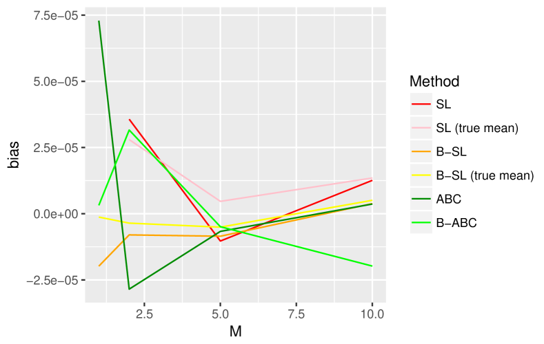
(a) Estimated bias of posterior mean estimates.

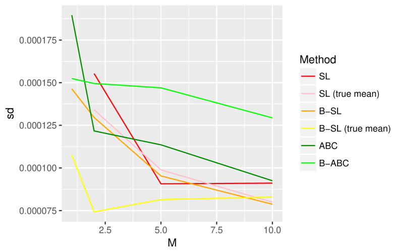
(b) Estimated standard deviation of posterior mean estimates.

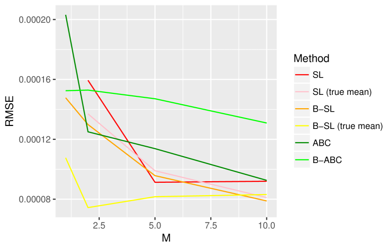
(c) Estimated RMSE of posterior mean estimates.

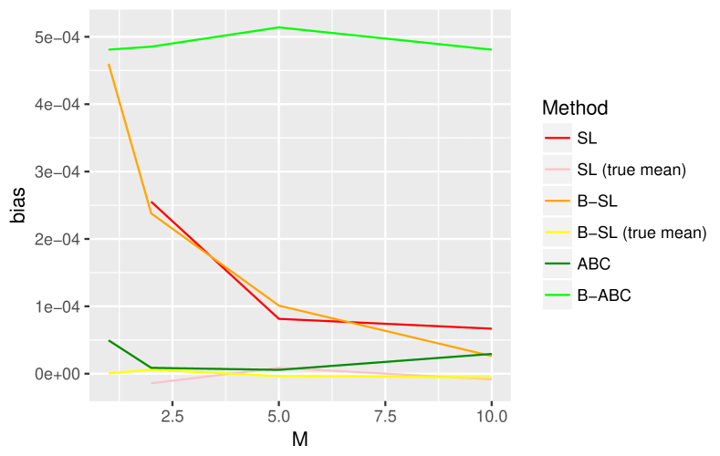
(d) Estimated bias of posterior standard deviation estimates.

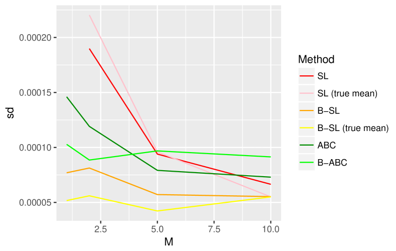
(e) Estimated standard deviation of posterior standard deviation estimates.

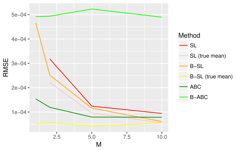
(f) Estimated RMSE of posterior standard deviation estimates.

Figure 1: Estimated bias, standard deviation and RMSE from standard and bootstrapped versions of SL and ABC.

Figure 2 compares the efficiency of posterior mean and standard deviation estimates from MCMC using different BLB-SL approximations. We observe that the subsampling has two large effects (both of which are increased by decreasing the size of the subsample): the posterior s.d. is overestimated (see figure 2(d)); and the variance of the estimates is increased (due to an increased autocorrelation in the chains). However, we observe that both of these effects are reduced dramatically by using the true value of $\mu_{\theta}$ in the SL estimates. In this situation, the autocorrelation in the MCMC chains and the errors in posterior estimates are similar between B-SL and BLB-SL, no matter the size of the subsample (for $n=10,000$, $1000$ or $100$). This suggests great potential for the BLB approach, as long as accurate estimates of $\mu_{\theta}$ may be obtained through other means. Section 3.3 illustrates that the regression approach suggested in section 2.3 provides a way of achieving this.

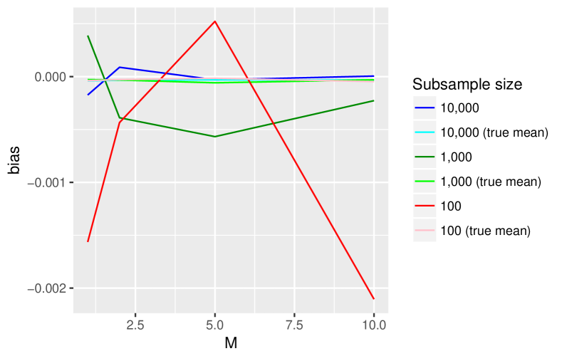
(a) Estimated bias of posterior mean estimates.

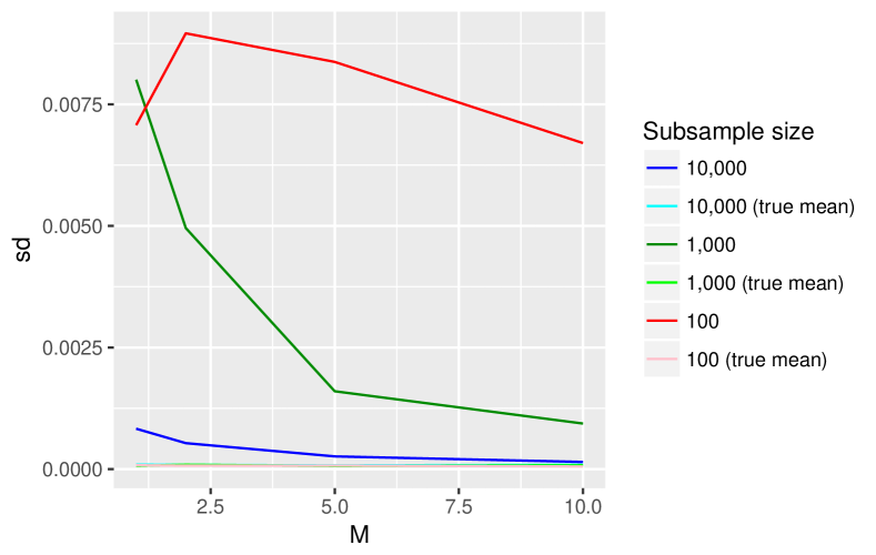
(b) Estimated standard deviation of posterior mean estimates.

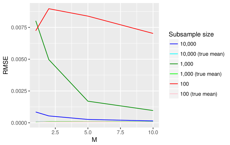
(c) Estimated RMSE of posterior mean estimates.

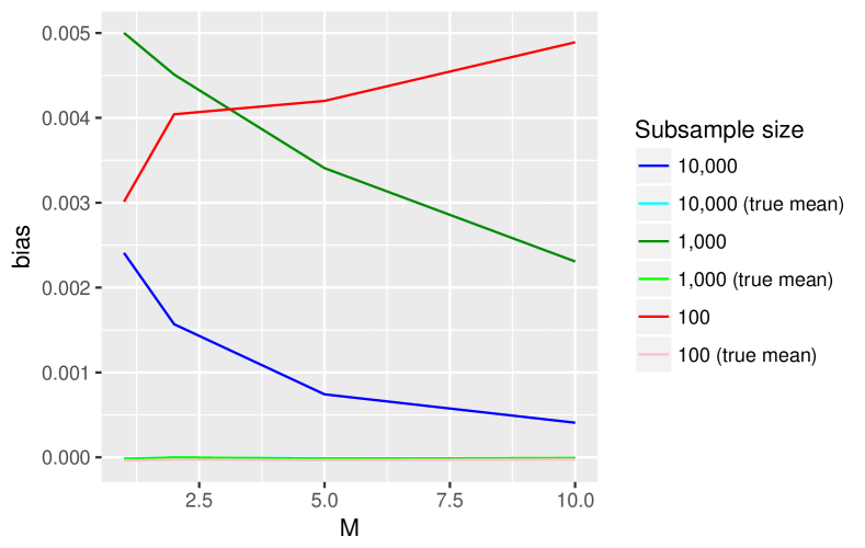
(d) Estimated bias of posterior standard deviation estimates.

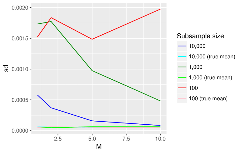
(e) Estimated standard deviation of posterior standard deviation estimates.

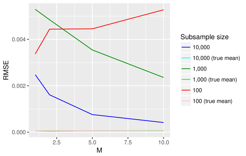
(f) Estimated RMSE of posterior standard deviation estimates.

Figure 2: Estimated bias, standard deviation and RMSE from BLB-SL samplers.

3.2 Lotka-Volterra model

3.2.1 Introduction

The Lotka-Volterra model is well-studied in the ABC literature. The model is a stochastic Markov jump process that describes how the number of individuals in two populations (one of predators, the other of prey) change over time. We use the form of the model in Wilkinson (2013), in which $X$ represent the number of predators and $Y$ the number of prey. The following reactions may take place:

• A prey may be born, with rate $\theta_{1}Y$, increasing $Y$ by one.

• The predator-prey interaction in which $X$ increases by one and $Y$ decreases by one, with rate $\theta_{2}XY$.

• A predator may die, with rate $\theta_{3}X$, decreasing $X$ by one.

Figure 4(a) shows the simulated data $y$ studied in this section: it consists of two oscillating time series: one giving the size of the predator population, the other of the prey. The simulation starts with initial populations $X=50$ and $Y=100$, and including the initial values has 32 measurements for each series, with the values of $X$ and $Y$ being recorded every 2 time units. The model may be simulated exactly using the Gillespie algorithm (Gillespie, 1977), but it is not possible to evaluate its likelihood. We followed the ABC approaches in Wilkinson (2013); Papamakarios and Murray (2016), using as summary statistics a 9-dimensional vector composed of the mean, log variance and first two autocorrelations of each time series, together with the cross-correlation between them (scaled by dividing by the summary statistic vector $T$ of the observed data).

This model has a number of properties that provide a challenge to our proposed approach:

1. The simulations from the model give temporal data, which requires the use of the block bootstrap (as described in section 2.1.3).

2. The simulations from the model cannot always be considered to be stationary time series, since sometimes (more commonly for inappropriate parameters) the sizes of the populations decreases to zero, or diverges towards infinity. We do not treat such simulations differently to any other simulation, thus our results help to illustrate how robust our approach is to this situation.

3. The 9-dimensional summary statistics allow us to illustrate the performance of our bootstrapping approach for estimating a covariance matrix.

4. The distribution of the summary statistics is not close to being Gaussian, and there are complex dependencies between the statistics (see figure 3). The former point allows us to examine the performance of SL when the Gaussian assumption is not satisfied (as previously studied in Price et al. (2017); the latter suggests that the approach of Meeds and Welling (2014) may not be appropriate, since they assume a diagonal covariance matrix.

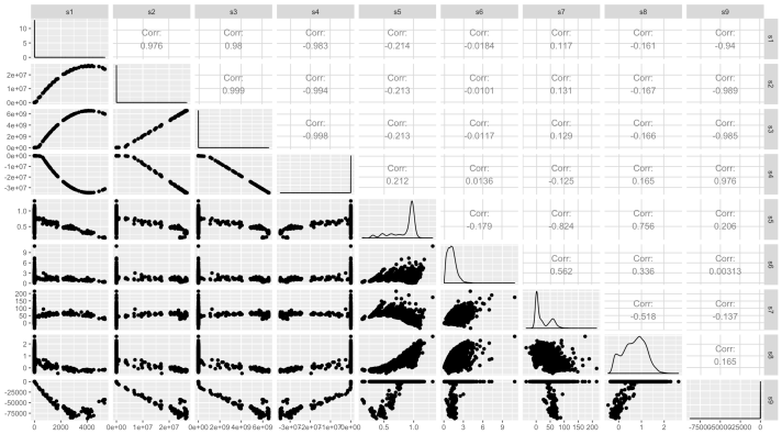
Figure 3: Scatter plots and kernel density estimates from draws from the distribution of the summary statistics conditional on the true parameters, and estimated correlations between the statistics.

We compared the output of MCMC algorithms employing the approximate likelihoods given by SL, B-SL, ABC and B-ABC. We ran each method with several different choices of $M$, and the bootstrap algorithms used $R=100$ resamples. The algorithms were run for $5\times 10^{4}$ iterations, and were initialised at the parameters $\theta_{1}=1$, $\theta_{2}=0.005$ and $\theta_{3}=0.6$ for which the data $y$ was simulated. The MCMC proposal was a multivariate Gaussian with diagonal covariance matrix whose diagonal is $\left(0.2^{2},0.001^{2},0.2^{2}\right)$, these values being determined using pilot runs. Our prior followed Wilkinson (2013), being uniform in the $\log$ domain

$$p\left(\log\left(\theta\right)\right)\propto\prod_{i=1}^{3}\mathcal{U}\left(\log\left(\theta_{i}\right)\mid\text{lower}=-6,\text{upper}=2\right).$$

The block bootstrap used blocks of length 8, so that each bootstrap resample consists of 4 blocks. Each statistic of each resample is calculated by combining the corresponding statistic of each of the constituent blocks in the obvious way.

3.2.2 Results

Table 1 shows the mean (over the three parameters) estimated IAT of each sampler, and figure 4 (b-f) shows kernel density estimates of the marginal posterior distributions based on the MCMC samples. In comparing the results from standard SL to standard ABC, we see that SL usually results in more efficient MCMC samplers, and we do not see any clear indications that the Gaussian assumption made in SL is problematic. The bootstrapped algorithms do not appear to be adversely affected by any of the challenges described in the previous section, giving similar posterior distributions to the standard approaches. Further, the autocorrelation properties of the MCMC chains from the bootstrapped algorithms are improved over their standard counterparts. This provides further evidence for the observation made in section 3.1 that the bootstrapped methods are useful when the corresponding standard estimates of the likelihood have a high variance.

Bootstrapped SL consistently exhibits the best performance: figure 4(d) shows that the low IAT found for SL when $M=5$ is not representative of the performance of the algorithm, since the sampler is only exploring a region in the tails of the posterior.

Algorithm	$M=1$	$M=2$	$M=5$	$M=10$	$M=50$
SL	N/A	3749	273	4210	326
B-SL	3543	1141	504	190	168
ABC $\epsilon=0.1$	6006	2969	4813	4506	1974
B-ABC $\epsilon=0.1$	5443	2874	1409	496	199
ABC $\epsilon=0.2$	13124	2923	2223	1416	427

Table 1: The estimated integrated autocorrelation time (to 0 d.p.) of each chain.

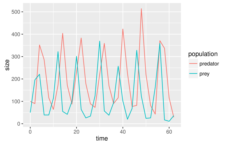
(a) Data simulated from the Lotka-Volterra model.

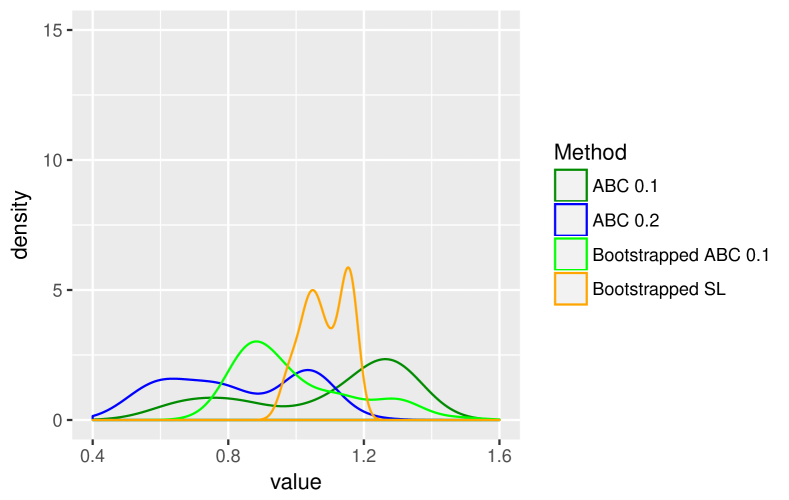
(b) Density estimates for $M=1$.

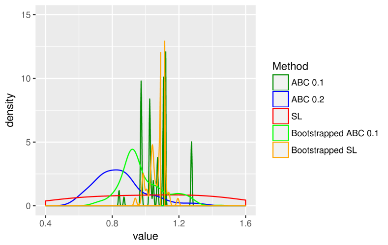
(c) Density estimates for $M=2$.

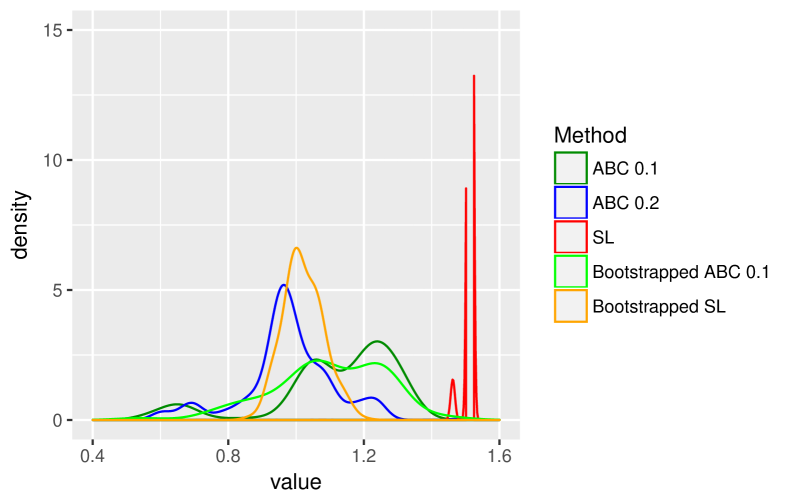
(d) Density estimates for $M=5$.

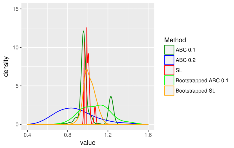
(e) Density estimates for $M=1$0.

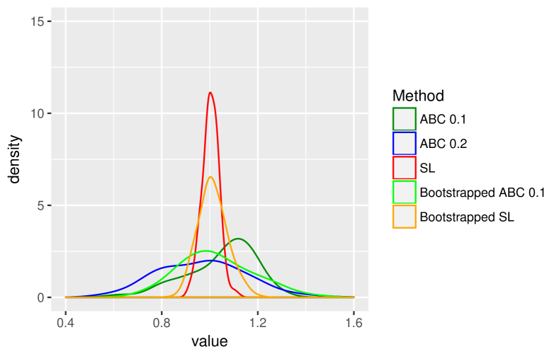
(f) Density estimates for $M=5$0.

Figure 4: SL and ABC algorithms applied to the Lotka-Volterra model.

3.3 Ising model

Undirected graphical models, or Markov random fields (MRFs), have previously been studied using ABC in a number papers, beginning with Grelaud et al. (2009). Such models have the form

$$L_{\theta}\left(y\right)=\frac{\gamma_{\theta}\left(y\right)}{Z\left(\theta\right)},$$

where $\gamma_{\theta}\left(y\right)$ is tractable, but the partition function $Z\left(\theta\right)$ cannot, in practice, be evaluated pointwise. Møller et al. (2006); Murray et al. (2006) pioneered the approach of estimating $L_{\theta}$ at each $\theta$ using importance sampling (known as auxiliary variable methods), embedded in an MCMC algorithm to perform Bayesian inference on $\theta$. ABC may be used as an alternative, but the likelihood estimates are typically high variance in comparison with those from the Møller et al. (2006) approach (Everitt et al. (2017) establishes a connection between the two approaches). However, when using a latent MRF model, ABC can be competitive with auxiliary variable methods (Everitt and Rowińska, 2017). Also, SL provides a lower variance alternative to ABC that can be competitive with auxiliary variable methods (Moores et al., 2015; Everitt et al., 2017). All of these previous approaches require simulating from $L_{\theta}$, which for most MRFs needs to be done approximately by using a run of MCMC with $L_{\theta}\left(\cdot\right)$ as the target distribution (Caimo and Friel, 2011). The use of MCMC introduces an approximation, which is small as long the chain is run long enough to have essentially forgotten its initial condition (Everitt, 2012).

In this section, we focus on the Ising model. This is a pairwise Markov random field model on binary variables, each taking values in $\left\{-1,1\right\}$. Its distribution is given by

$$L_{\theta}\left(y\right)\propto\exp\left(\theta\sum_{\left(i,j\right)\in\mathbf{N}}y_{i}y_{j}\right),$$

where $\theta_{x}\in\mathbb{R}$, $x_{i}^{h}$ denotes the $i$th random variable in $x^{h}$ and where $\mathbf{N}$ is a set that defines pairs of nodes that are “neighbours”. We consider the case where the neighbourhood structure is given by a regular 2-dimensional grid, using a first order model (so that variables horizontally and vertically adjacent are neighbours) and toroidal boundary conditions, and use a Gibbs sampler to simulate from $L_{\theta}\left(\cdot\right)$. The mixing properties of the Gibbs sampler on Ising models are well understood, and indicate a limitation of all of the approaches to inference outlined above: namely that the approaches do not scale to large MRFs. The mixing time of Gibbs samplers on Ising models on 2-d grids is at best polynomial in the number of rows in the grid (Lubetzky and Sly, 2012). Therefore, as the size of the grid grows, in addition to the number of single variable updates growing linearly in the size of the grid, we expect to need to run the Gibbs sampler for more iterations.

In this section we study data from a $1,000\times 1,000$ Ising model (so that $N=10^{6}$), generated with $\theta=0.3$, and compare results from the exchange algorithm (an auxiliary variable MCMC approach introduced in Murray et al. (2006)) and BLB-SL. In all cases, the Gibbs sampler for simulating from the likelihood is burned in for 10 iterations. The exchange algorithm was initialised at $\theta=0.298$ and run for $1000$ iterations, using a normal proposal with standard deviation $0.001$. For BLB-SL, the spatial block bootstrap was used (as described in section 2.1.3), with the size of the subsample being either $100\times 100$ or $50\times 50$ (so that $n=10^{4}$ or $2,500$) and the block size being $50\times 50$ or $25\times 25$ (so that $B=2,500$ or $625$). The (sufficient) statistic $S\left(y\right)=\sum_{\left(i,j\right)\in\mathbf{N}}y_{i}y_{j}$ was used, and we took $M=1$. The SMC algorithm from section 2.3 was used, with $P=1,000$ particles and $T=10$ target distributions, with $\nu_{t}=\left(t/T\right)^{2}$. For each $\theta_{t}^{(p)}$ (the $p$th particle at the $t$th target) a sample $x_{t}^{(p)}$ of size $\sqrt{n}\times\sqrt{n}$ is simulated from $l_{\theta}\left(\cdot\right)$. $\mu_{\theta}$ and $\Sigma_{\theta}$ was then approximated as follows.

• Calculate $\left(N/n\right)S_{n}$ (the statistic rescaled from a grid of size $n$ to a grid of size $N$) as a “raw” estimate of $\mu_{\theta}$. Find the $C$ closest $\theta$ values to $\theta_{t}^{(p)}$ (including $\theta_{t}^{(p)}$ itself) and perform a linear regression of $\left(N/n\right)S_{n}$ on $\theta_{t}^{(p)}$. Then, from the regression use the predicted value of the response at $\theta_{t}^{(p)}$ as the estimate of $\mu_{\theta}$.

• Compose $R=100$ resamples from $x_{t}^{(p)}$ by using the following procedure

  • Take (overlapping) blocks of size $\sqrt{B}\times\sqrt{B}$ from $x_{t}^{(p)}$ as described in the spatial block bootstrap: there are $(1+\sqrt{B})\times(1+\sqrt{B})$ of these blocks in total. Compute the statistic for each block, denoting it by $\mathcal{S}_{b}$ for the $b$th block.

  • Randomly compose a resample of size $\sqrt{N}\times\sqrt{N}$ by piecing together $N/B$ blocks. The indices $\mathcal{B}$ of the blocks used in the resample may be the same for all $p$ and $t$, thus can be generated in a pre-processing step.

• Compute the statistic for each resample, using for the $r$th resample

  $$S_{N}^{(r)}=\left(\frac{N}{N-\frac{N}{\sqrt{B}}}\right)\sum_{b\in\mathcal{B}}\mathcal{S}_{b},$$

  where the rescaling accounts for the absence of edges between the blocks. The sample variance of the $\left\{S_{N}^{(r)}\right\}_{r=1}^{R}$ is then our approximation of $\Sigma_{\theta}$ from the block-BLB.

Figure 5(a) shows the estimated posterior distributions from the exchange algorithm, and runs of the BLB-SL SMC method for different values of $C$ and $n$. We observe that the posterior distribution from the exchange algorithm is very well approximated by the posterior distribution from BLB-SL SMC when $C=100$ and $n=10,000$, with the posterior standard deviation being overestimated for smaller $C$. This is due to the increasing variance estimates of the SL mean as $C$ decreases, as was previously observed in section 3.1. In this example, the combination (through regression) of $C=100$ raw estimates of $\mu_{\theta}$ is sufficient to reduce the variance sufficiently that an accurate posterior results. This variance reduction, without the introduction of significant bias, is possible since the assumptions made in the regression are appropriate. Figure 5(c) illustrates shows the raw estimates of $\mu_{\theta}$ against $\theta$ in the region of the posterior, together with the predicted regression with $C=100$ for each point. We also find that using $C=200$ and $n=2,500$ yields a fairly accurate posterior, indicating that our approach can be accurate even when the subsampling ratio $N/n$ is quite large ($400$ in this case). Figure 5(b) shows the effective sample size (ESS) over the iterations of the SMC sampler for different values of $C$. As in section 3.1 we observe that the efficiency of the Monte Carlo method in which the BLB-SL estimate is embedded decreases when the estimates of the mean have higher variance. For comparison, the ESS for the exchange algorithm was estimated at $98$ using the LaplacesDemon package in R (whilst recalling that the ESS is defined differently for importance sampling and MCMC algorithms).

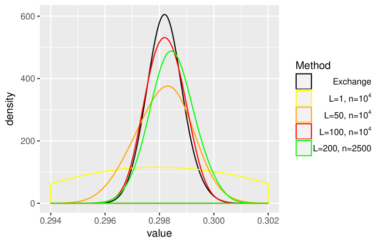
(a) Density estimates from each of the Monte Carlo algorithms.

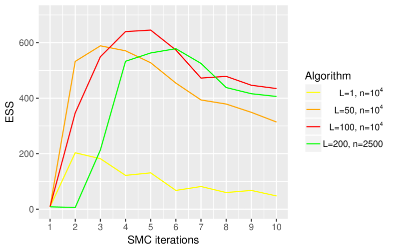
(b) The ESS over SMC iterations for the BLB-SL algorithms.

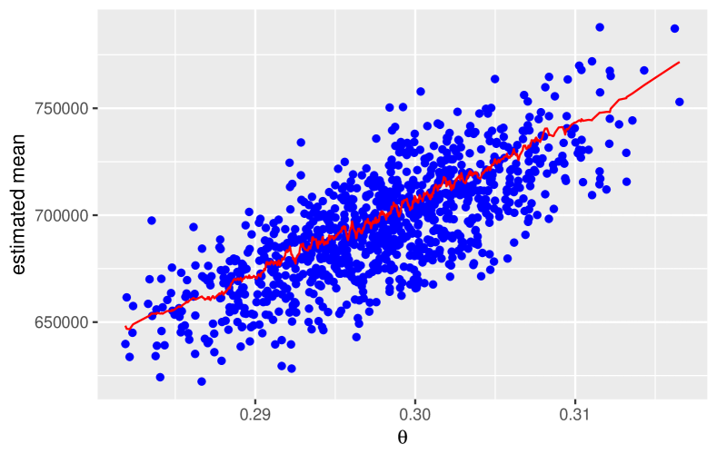
(c) Raw estimates of $\mu_{\theta}$(blue) and the locally linear regression prediction (red) with $L=1$00.

Figure 5: Results of applying BLB-SL to the Ising model.

4 Conclusions

This paper introduces methodology for improving the performance of SL in cases where a bootstrap may be used to estimate the variance of the chosen statistics. Further, it provides a method for using SL in “tall data” settings, where subsampling may be used such that the cost of the sampling algorithm depends on the size $n$ of the subsets rather than $N$, the size of the full data. In summary

• In situations in which the likelihood is difficult to estimate, bootstrap approximations of the variance of a statistic result in lower variance likelihood estimates, thus improve the efficiency of Monte Carlo methods that use SL. Further, using the bootstrap only results in a small bias. The same is true to an extent when using bootstrapped estimates of the ABC likelihood.

• Using the BLB to estimate the variance of a statistic has a similar performance to using the bootstrap, paving the way for using subsampling to estimate SLs. However, estimates of the mean of the statistic using subsamples are too high variance to result in either accurate approximations of the true posterior distribution, or low variance Monte Carlo algorithms.

• When using the BLB, regression estimates of the statistic mean may be used in order to reduce the variance sufficiently that an accurate approximation to the true posterior is obtained, even for large values of $N/n$. In this paper a local linear regression was used, but in other models different regression techniques such as Gaussian processes may be more appropriate.

The methods in this paper should be of use whenever a bootstrap method is available to estimate the variance of the chosen statistics, with the BLB being applicable to stationary models. It is possible that, since it only requires the simulation of subsamples of size $n$, BLB-SL may be useful in big data settings where ABC/SL would not usually be applied. One further remark about the big data setting is that often in such cases sophisticated Monte Carlo methods are not required since the posterior is approximately Gaussian. This is not necessarily the case in many models where ABC/SL might be used, since parameters are often non-identifiable, leading to complex posterior distributions no matter how much data is observed (see the differential equation models in Maybank et al. (2017), for example).

References

- Akeret et al. (2015) Akeret, J., Refregier, A., Amara, A., Seehars, S., and Hasner, C. (2015). Approximate Bayesian Computation for Forward Modeling in Cosmology. arXiv.
- Alquier et al. (2016) Alquier, P., Friel, N., Everitt, R. G., and Boland, A. (2016). Noisy Monte Carlo: Convergence of Markov chains with approximate transition kernels. Statistics and Computing 26(1), 29–47.
- An et al. (2016) An, Z., Drovandi, C. C., and Nott, D. J. (2016). Accelerating Bayesian Synthetic Likelihood with the Graphical Lasso.
- Andrieu and Roberts (2009) Andrieu, C. and Roberts, G. O. (2009). The pseudo-marginal approach for efficient Monte Carlo computations. The Annals of Statistics 37(2), 697–725.
- Andrieu and Vihola (2014) Andrieu, C. and Vihola, M. (2014). Establishing some order amongst exact approximations of MCMCs. arXiv, 1–20.
- Bardenet et al. (2017) Bardenet, R., Doucet, A., and Holmes, C. (2017). On Markov chain Monte Carlo methods for tall data. Journal of Machine Learning Research, 18, 1–43.
- Beaumont et al. (2002) Beaumont, M. A., Zhang, W., and Balding, D. J. (2002). Approximate Bayesian computation in population genetics. Genetics 162(4), 2025–35.
- Bentley (1975) Bentley, J. L. (1975). Multidimensional binary search trees used for associative searching. Communications of the ACM 18(9), 509–517.
- Buzbas and Rosenberg (2015) Buzbas, E. O. and Rosenberg, N. A. (2015). AABC: approximate approximate Bayesian computation when simulating a large number of data sets is computationally infeasible. Theoretical Population Biology, 99, 31–42.
- Caimo and Friel (2011) Caimo, A. and Friel, N. (2011). Bayesian inference for exponential random graph models. Social Networks, 33, 41–55.
- Del Moral et al. (2006) Del Moral, P., Doucet, A., and Jasra, A. (2006). Sequential Monte Carlo samplers. Journal of the Royal Statistical Society: Series B 68(3), 411–436.
- Drovandi et al. (2015) Drovandi, C. C., Moores, M. T., and Boys, R. J. (2015). Accelerating Pseudo-Marginal MCMC using Gaussian Processes.
- Efron (1979) Efron, B. (1979). Bootstrap Methods: Another Look At The Jackknife. The Annals of Statistics 7(1), 1–26.
- Everitt (2012) Everitt, R. G. (2012). Bayesian Parameter Estimation for Latent Markov Random Fields and Social Networks. Journal of Computational and Graphical Statistics.
- Everitt et al. (2017) Everitt, R. G., Johansen, A. M., Rowing, E., and Evdemon-Hogan, M. (2017). Bayesian model comparison with un-normalised likelihoods. Statistics and Computing 27(2), 403–422.
- Everitt et al. (2017) Everitt, R. G., Prangle, D., Maybank, P., and Bell, M. (2017). Auxiliary variable marginal SMC for doubly intractable models. arXiv, 1–18.
- Everitt and Rowińska (2017) Everitt, R. G. and Rowińska, P. A. (2017). Delayed acceptance ABC-SMC. arXiv, 1–18.
- Ghurye and Olkin (1969) Ghurye, S. G. and Olkin, I. (1969). Unbiased Estimation of Some Multivariate Probability Densities and Related Functions. The Annals of Mathematical Statistics 40(4), 1261–1271.
- Gillespie (1977) Gillespie, D. T. (1977). Exact stochastic simulation of coupled chemical reactions. Journal of Physical Chemistry 8(25), 2340–2361.
- Grelaud et al. (2009) Grelaud, A., Robert, C. P., and Marin, J.-M. (2009). ABC likelihood-free methods for model choice in Gibbs random fields. Bayesian Analysis 4(2), 317–336.
- Gutmann and Corander (2016) Gutmann, M. U. and Corander, J. (2016). Bayesian Optimization for Likelihood-Free Inference of Simulator-Based Statistical Models. Journal of Machine Learning Research 17(1), 4256–4302.
- Horowitz (2001) Horowitz, J. L. (2001). The bootstrap. Handbook of Econometrics 5(3159–3228).
- Jennings and Madigan (2017) Jennings, E. and Madigan, M. (2017). astroABC: An Approximate Bayesian Computation Sequential Monte Carlo sampler for cosmological parameter estimation. arXiv.
- Kleiner et al. (2014) Kleiner, A., Talwalkar, A., Sarkar, P., and Jordan, M. I. (2014). A scalable bootstrap for massive data. Journal of the Royal Statistical Society Series B 76(4), 795–816.
- Kreiss and Lahiri (2012) Kreiss, J.-P. and Lahiri, S. N. (2012). Bootstrap Methods for Time Series, Volume 30. Elsevier B.V.
- Kunsch (1989) Kunsch, H. R. (1989). The Jackknife and the Bootstrap for General Stationary Observations. The Annals of Statistics 17(3), 1217–1241.
- Kypraios et al. (2017) Kypraios, T., Neal, P., and Prangle, D. (2017). A tutorial introduction to Bayesian inference for stochastic epidemic models using Approximate Bayesian Computation. Mathematical Biosciences, 287, 42–53.
- Laptev et al. (2012) Laptev, N., Zaniolo, C., and Lu, T.-C. (2012). BOOT-TS: A Scalable Bootstrap for Massive Time-Series Data. NIPS Proceedings, 1–5.
- Lubetzky and Sly (2012) Lubetzky, E. and Sly, A. (2012). Critical Ising on the Square Lattice Mixes in Polynomial Time. Communications in Mathematical Physics 313(3), 815–836.
- Martin et al. (2017) Martin, G. M., Mccabe, B. P. M., Frazier, D. T., Maneesoonthorn, W., and Robert, C. P. (2017). Auxiliary Likelihood-Based Approximate Bayesian Computation in State Space Models. arXiv.
- Maybank et al. (2017) Maybank, P., Bojak, I., and Everitt, R. G. (2017). Fast approximate Bayesian inference for stable differential equation models.
- Meeds and Welling (2014) Meeds, E. and Welling, M. (2014). GPS-ABC: Gaussian process surrogate approximate Bayesian computation. Proceedings of the 30th Conference on Uncertainty in Artificial Intelligence.
- Møller et al. (2006) Møller, J., Pettitt, A. N., Reeves, R. W., and Berthelsen, K. K. (2006). An efficient Markov chain Monte Carlo method for distributions with intractable normalising constants. Biometrika 93(2), 451–458.
- Moores et al. (2015) Moores, M. T., Mengersen, K., Drovandi, C. C., and Robert, C. P. (2015). Pre-processing for approximate Bayesian computation in image analysis. Statistics and Computing 25(1), 23–33.
- Murray et al. (2006) Murray, I., Ghahramani, Z., and MacKay, D. J. C. (2006). MCMC for doubly-intractable distributions. In UAI, pp. 359–366.
- Papamakarios and Murray (2016) Papamakarios, G. and Murray, I. (2016). Fast Epsilon-Free Inference of Simulation Models with Bayesian Conditional Density Estimation. arXiv.
- Peters et al. (2010) Peters, G. W., Wuthrich, M. V., and Shevchenko, P. V. (2010). Chain Ladder Method: Bayesian Bootstrap versus Classical Bootstrap. Insurance: Mathematics and Economics 47(1), 36–51.
- Pollock et al. (2016) Pollock, M., Fearnhead, P., Johansen, A. M., and Roberts, G. O. (2016). The Scalable Langevin Exact Algorithm: Bayesian Inference for Big Data. arXiv, 1–47.
- Prangle et al. (2017) Prangle, D., Everitt, R. G., and Kypraios, T. (2017). A rare event approach to high dimensional approximate Bayesian computation. Statistics and Computing.
- Price et al. (2017) Price, L. F., Drovandi, C. C., Lee, A., and Nott, D. J. (2017). Bayesian Synthetic Likelihood. Journal of Computational and Graphical Statistics.
- Pritchard et al. (1999) Pritchard, J. K., Seielstad, M. T., Perez-Lezaun, A., and Feldman, M. W. (1999). Population growth of human Y chromosomes: a study of Y chromosome microsatellites. Molecular Biology and Evolution 16(12), 1791–8.
- Sherlock et al. (2017) Sherlock, C., Golightly, A., and Henderson, D. A. (2017). Adaptive, delayed-acceptance MCMC for targets with expensive likelihoods. Journal of Computational and Graphical Statistics 26(2), 434–444.
- van der Vaart et al. (2015) van der Vaart, E., Beaumont, M. A., Johnston, A. S. A., and Sibly, R. M. (2015). Calibration and evaluation of individual-based models using Approximate Bayesian Computation. Ecological Modelling, 312, 182–190.
- Vo et al. (2015) Vo, B. N., Drovandi, C. C., and Pettitt, A. N. (2015). Bayesian parametric bootstrap for models with intractable likelihoods.
- Wilkinson (2013) Wilkinson, D. J. (2013). Summary Stats for ABC.
- Wilkinson (2014) Wilkinson, R. D. (2014). Accelerating ABC methods using Gaussian processes. AISTATS, 1015–1023.
- Wood (2010) Wood, S. N. (2010). Statistical inference for noisy nonlinear ecological dynamic systems. Nature 466(August), 1102–1104.
- Zhu et al. (2016) Zhu, W., Marin, J. M., and Leisen, F. (2016). A Bootstrap Likelihood approach to Bayesian Computation. Australian & New Zealand Journal of Statistics 58(2), 227–244.