Laser pulse probe of the chirality of Cooper pairs

Abstract

The internal chirality of Cooper pairs is shown to modify strongly the response of a superconductor to the local heating by a laser beam. The suppression of the chiral order parameter inside the hot spot appears to induce the supercurrents flowing around the spot region. The chirality affects also the sequential stage of thermal quench developing according to the Kibble-Zurek scenario: besides the generation of vortex–antivortex pairs the quench facilitates the formation of superconducting domains with different chirality. These fingerprints of the chiral superconducting state can be probed by any experimental techniques sensitive to the local magnetic field. The supercurrents encircling the hot spot originate from the inhomogeneity of the state with the broken time reversal symmetry and their detection would provide a convenient alternative to the search of the spontaneous edge currents sensitive to the boundary properties. Thus, the suggested setup can help to resolve the long-standing problem of unambiguous detection of type of pairing in $\mathrm{Sr_{2}RuO_{4}}$ considered as a good candidate for chiral superconductivity.

I Introduction

The interaction of light with different types of orderings in condensed matter systems is in the focus of current research in the field of optoelectronics Kirilyuk et al. (2013, 2010); Fausti et al. (2011); Suda et al. (2015); Veshchunov et al. (2016). The light controlled manipulation of magnetic and/or superconducting states provides a perspective way to construct new fast operating switching devices Kirilyuk et al. (2013, 2010) and serves a basis for different experimental methods probing and characterizing the order parameter structure and dynamics Yuzbashyan et al. (2006); Matsunaga et al. (2014). In particular, remarkable progress has been recently achieved in the design of sensitive superconducting bolometers and photon detectors Semenov et al. (2001); Gol’tsman et al. (2001). Fundamental issues of the order parameter dynamics have been investigated probing the Higgs mode in the superconducting state Yuzbashyan et al. (2006); Matsunaga et al. (2014).

The simplest physical picture describing the effect of the light pulse on superconductor can be constructed starting from a so called “hot spot” model Semenov et al. (2001); Maingault et al. (2010); Zotova and Vodolazov (2012). Within this approach one can assume the energy of the laser pulse to be transferred to the electronic subsystem which results in further formation of the locally heated state with an increased electronic temperature. This increase in the local temperature is responsible for the partial or complete suppression of the superconducting order parameter in the region of the hot spot. The state with the inhomogeneous temperature is unstable due to the heat diffusion and at the next stage the hot spot disappears and the order parameter relaxes to its initial value before the light pulse absorption. The exact picture depends of course on the electron-electron and electron-phonon relaxation rates which are responsible for different stages of the evolution of the nonequilibrium electronic distribution. Provided the relaxation stage is rather short and can be considered as a rapid thermal quench the thermodynamic order parameter fluctuations can complicate the return to the initial state giving rise to the formation of the vortex - antivortex pairs according to the Kibble-Zurek scenario Kibble (1976); H. Zurek (1985); Volovik (2000); Maniv et al. (2003).

Should we expect any essential changes in the above model if the superconducting order parameter is not just a single complex function but may have several components or possess a nontrivial anisotropy in the momentum space? In other words, does the study of the superconductor dynamics excited by the light pulse allows to distinguish the states with different internal structure of the Cooper pairs? The goal of the present paper is to develop a theoretical basis for the use of the laser beam as a probe of such unconventional superconducting states, more specifically the states with a nonzero internal average angular momentum of the Cooper pairs $\mathbf{L}$. It is instructive to start our discussion of the appropriate generalization of the hot spot model from a qualitative analysis of inhomogeneous states for $\mathbf{L}\neq 0$. The angular momentum of the relative motion of two electrons in the pair naturally interacts with the angular momentum of the motion of the pair center of mass. For any inhomogeneity of the superconducting state this interaction of the angular momenta can induce the supercurrents and corresponding magnetic field. Naively, one can expect these supercurrents to be proportional to the effective magnetization currents of the Cooper pairs: $\propto\mathop{\mathrm{curl}}\mathbf{L}$. However the orbital angular momentum of the sample bulk appears to be significantly reduced compared to expected $N\hbar/2$ value where $N$ is the total amount of electrons in a volume. The orbital momentum of the bulk is determined by the contribution of the Cooper pairs which are smaller than the inter–pair distance so the momentum is reduced by factor $(T_{c}/E_{F})^{2}$ Volovik and Mineev (1981). A more precise analysis gives additional logarithmic factor and final expression has a form $L_{z}\propto\hbar N(T_{c}/E_{F})^{2}\ln(E_{F}/T_{c})$ Volovik (1975); Cross (1975). A noticeable contribution to the supercurrent is provided by another mechanism, namely by the mixture of several order parameter components generated by the order parameter inhomogeneity. Such mixture originates from the obvious fact that the projection of the internal angular momentum can not conserve in the presence of the inhomogeneity. Previously, the search of the corresponding spontaneous currents was mainly related to the edge of the samples. Unfortunately, near the edge the order parameter inhomogeneity and, thus, the generation of the additional order parameter components and the resulting supercurrents strongly depend on the details of the electron scattering at the surface, i.e. on the surface quality Sauls (2011); Lederer et al. (2014); Huang et al. (2015); Bakurskiy et al. (2017). As a consequence, the edge currents can be strongly diminished and surface imperfections may cause the difficulties in their experimental observation in $\mathrm{Sr_{2}RuO_{4}}$ Kirtley et al. (2007) which is considered to be a most promising candidate for a superconductor with the chiral $p$-wave order parameter Kallin (2012). The other explanations of the edge currents absence focus on possibility of chiral non $p$-wave pairing type in $\mathrm{Sr_{2}RuO_{4}}$ Scaffidi and Simon (2015) for which the macroscopic orbital momentum vanishes in the finite size samples Huang et al. (2014); Tada et al. (2015); Volovik (2014). Also the properties of the edge currents appear to depend on the band structure of $\mathrm{Sr_{2}RuO_{4}}$ Bouhon and Sigrist (2014); Imai et al. (2013).

From this point of view the order parameter inhomogeneity created by the laser beam far from the sample edge of uncontrolled quality provides much better conditions for the study of the above supercurrents. The current circulating around the hot spot (see Fig. 1) should be easily detected by any experimental techniques sensitive to small local magnetic field such as SQUID microscope or sensitive Hall sensor. The generation of the magnetic field in the inhomogeneously heated samples is common for the systems with the broken time reversal symmetry. For example the magnetic field appears in the hot spots in multiband $s+is$ and $s+id$ superconductors Garaud et al. (2016). The generation of the secondary order parameter components can be even more pronounced at the late stage of the hot spot evolution. Indeed, provided the spot dimension exceeds the coherence length one can expect that the rather fast quench to the initial temperature can be accompanied by nucleation of different order parameter components forming, thus, a domain structure in addition to the well-known vortex-antivortex configurations induced by the Kibble–Zurek mechanism.

For the further quantitative analysis of the above phenomena we choose a rather general two-component Ginzburg–Landau model introduced previously in a number of works Heeb and Agterberg (1999); Barash and Mel’nikov (1991) for the description of properties of the $\mathrm{Sr_{2}RuO_{4}}$ compound Heeb and Agterberg (1999); Vadimov and Silaev (2013).

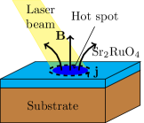
Figure 1: (Color online) The proposed experimental setup. The laser beam heats the sample inducing the supercurrents flowing around the hot spot. The magnetic field created by these currents can be observed by the SQUID microscope or the Hall sensor.

In the Section II we introduce Ginzburg–Landau free energy and the main equations describing the superconducting state. For the case of a smooth order parameter profile in the hot spot these equations are solved in the Section III. The final expression for the magnetic field is obtained for the Gaussian profile of temperature. The Section IV is devoted to superconductor dynamics in the thermal quench mode and study of the chiral domain generation according to the Kibble–Zurek mechanism. The stability of the domains and their interaction with the vortices is discussed in the Section V. In the final Section VI we sum up the results of this paper.

II Model

The superconducting order parameter has two components $(\Psi_{+},\Psi_{-})$ which stand for the Cooper pairs with opposite direction of internal orbital momentum. The free energy of the superconductor is given by the following expressionHeeb and Agterberg (1999):

$$F=\int\left\{-a\left(|\Psi_{+}|^{2}+|\Psi_{-}|^{2}\right)+\frac{b_{1}}{2}\left(|\Psi_{+}|^{2}+|\Psi_{-}|^{2}\right)^{2}+\right.\\ b_{2}\left|\Psi_{+}\Psi_{-}\right|^{2}+\\ K_{1}\left(|D_{+}\Psi_{+}|^{2}+|D_{-}\Psi_{+}|^{2}+|D_{+}\Psi_{-}|^{2}+|D_{-}\Psi_{-}|^{2}\right)+\\ K_{2}|D_{+}\Psi_{-}+D_{-}\Psi_{+}|^{2}+\\ K_{3}\left[|D_{+}\Psi_{+}|^{2}+|D_{-}\Psi_{-}|^{2}+(D_{+}\Psi_{-})^{\ast}(D_{-}\Psi_{+})+c.c.\right]+\\ \left.\frac{\left(\mathop{\mathrm{curl}}\mathbf{A}\right)^{2}}{8\pi}\right\}\;d^{3}r\ ,$$ (1)

where $\mathbf{A}$ is the vector potential of the magnetic field, $\mathbf{D}=-i\nabla-2\pi/\Phi_{0}\mathbf{A}$ is the covariant derivative, $D_{\pm}=(D_{x}\pm iD_{y})/\sqrt{2}$, $\Phi_{0}$ is the superconducting flux quantum, $a$, $b_{1}$, $b_{2}$, $K_{1}$, $K_{2}$ and $K_{3}$ are the phenomenological parameters. The coefficient $a$ depends on the temperature as follows $a=\alpha(T_{c}-T)$. For simplicity we omitted the terms lowering the symmetry of the free energy to $D_{4h}$ symmetry, restricting ourselves to the case of $D_{6h}$ crystal.Also we assume that the spatial variations of the order parameter are only in $xy$ plane and neglect the variations along $z$-axis. If $b_{2}>0$ the equilibrium homogeneous states have form of chiral domains $(\Psi_{+},\Psi_{-})=(\sqrt{a/b_{1}},0)$ and $(\Psi_{+},\Psi_{-})=(0,\sqrt{a/b_{1}})$.

The laser pulse is absorbed by the electron subsystem of the superconductor inducing, thus, non-equilibrium distribution of the quasiparticles in the sample. In general case this distribution does not correspond to any temperature though if we suppose that the electron–electron scattering is the fastest process in the system the distribution of the quasiparticles rapidly thermalizes. Then one can introduce an inhomogeneous temperature $T(\mathbf{r})$ and the parameter $a$ also becomes a function of the coordinates $a=\alpha(T_{c}-T(\mathbf{r}))$. We suppose inhomogeneity to have a form of a hot spot and the temperature to be constant far from it, i.e. $a(\mathbf{r})\to a_{0}=\alpha(T_{c}-T_{0})$ at $r\to\infty$, where $T_{0}$ is the bath temperature. Introducing the dimensionless order parameter components $\eta_{\pm}=\Psi_{\pm}\sqrt{b_{1}/a_{0}}$ we rewrite the free energy:

$$F=\frac{H_{cm}^{2}}{4\pi}\int\left\{-\tau(|\eta_{+}|^{2}+|\eta_{-}|^{2})+\frac{1}{2}\left(|\eta_{+}|^{2}+|\eta_{-}|^{2}\right)+\right.\\ \beta|\eta_{+}\eta_{-}|^{2}+\xi^{2}\left(|\mathbf{D}\eta_{+}|^{2}+|\mathbf{D}\eta_{-}|^{2}\right)+\\ 2\xi^{2}\zeta\left[(D_{+}\eta_{-})^{\ast}(D_{-}\eta_{+})+c.c.\right]+\\ \left.\frac{\left(\mathop{\mathrm{curl}}\mathbf{A}\right)^{2}}{2H_{cm}^{2}}\right\}\;d^{3}r\ ,$$ (2)

where $H_{cm}=\sqrt{4\pi a_{0}^{2}/b_{1}}$ is the thermodynamical critical field, $\xi=\sqrt{(K_{1}+K_{2})b_{1}}/a_{0}$ is the coherence length, $\tau(\mathbf{r})=a(\mathbf{r})/a_{0}$ and $\zeta=K_{2}/(K_{1}+K_{2})$ and $\beta=b_{2}a_{0}^{2}/b_{1}^{2}$. Here we assume that $K_{2}-K_{3}$ is negligible due to the small electron–hole asymmetryBalatskii and Mineev (1985).

One can obtain the Ginzburg–Landau equations for the order parameter components:

$$\xi^{2}\left(\mathbf{D}^{2}\eta_{+}+2\zeta D_{+}^{2}\eta_{-}\right)-\tau\eta_{+}+\eta_{+}|\eta_{+}|^{2}+\\ (1+\beta)|\eta_{-}|^{2}\eta_{+}=0\ ,$$ (3)

$$\xi^{2}\left(\mathbf{D}^{2}\eta_{-}+2\zeta D_{-}^{2}\eta_{+}\right)-\tau\eta_{-}+\eta_{-}|\eta_{-}|^{2}+\\ (1+\beta)|\eta_{+}|^{2}\eta_{-}=0\ .$$ (4)

Varying the free energy functional over the vector potential $\mathbf{A}$ one can obtain the expression for the superconducting current:

$$\mathbf{j}_{s}=-\frac{c\Phi_{0}}{16\pi^{2}\lambda^{2}}\left\{\eta_{+}^{\ast}(\mathbf{D}\eta_{+})+\eta_{-}^{\ast}(\mathbf{D}\eta_{-})+\phantom{\sqrt{2}}\right.\\ \left.\zeta\sqrt{2}(\hat{\mathbf{x}}+i\hat{\mathbf{y}})\left[\eta_{-}(D_{-}\eta_{+})^{\ast}+\eta_{+}^{\ast}(D_{+}\eta_{-})\right]+c.c.\right\}\ ,$$ (5)

where $\lambda=\Phi_{0}/[4\sqrt{2\pi^{3}(K_{1}+K_{2})}]$ is the London penetration length. The first terms proportional to $\eta_{+}^{\ast}(\mathbf{D}\eta_{+})$ and $\eta_{-}^{\ast}(\mathbf{D}\eta_{-})$ are common for the Ginzburg–Landau theory of conventional superconductors. The rest two terms contain not only the contributions proportional to the superfluid velocities of the different order parameter components but also a non-zero contribution caused by the inhomogeneity of the magnitudes of the order parameter components. Below we show that the suppression of one of the order parameter components can generate another component and the corresponding superconducting current.

III Weak heating. Adiabatic approximation

We choose for definiteness a chiral domain with $\eta_{+}=1$ and $\eta_{-}=0$ and consider a hot spot located far from the domain boundaries. To elucidate our main results we start from a simplified “adiabatic” model assuming that the temperature varies slowly at the length scale $\xi$, i.e. $|\nabla\tau|\ll\tau/\xi$. Under these assumptions the dominating order parameter component $\eta_{+}$ “follows” the local temperature and the other order parameter component $\eta_{-}$ can be found as a perturbation:

$$\eta_{+}\approx\sqrt{\tau}e^{i\phi}\ ,$$ (6)

$$\eta_{-}\approx-\frac{2\zeta\xi^{2}D_{-}^{2}\eta_{+}}{\beta\tau}\ ,$$ (7)

where $\phi$ is the unknown phase. Also we assume that the sample is a thin film with the thinkness $d$ much smaller than the London penetration length $\lambda$. This simplification allows us to neglect the vector potential and the screening effects. For simplicity we assume that the temperature distribution is axi-symmetric $\tau(\mathbf{r})=\tau(r)$. Then we can omit the phase $\phi$ and find the order parameter components in the following form:

$$\eta_{+}(r)=\sqrt{\tau}=f_{+}(r)$$ (8)

$$\eta_{-}(r,\varphi)=\frac{\zeta\xi^{2}}{\beta\tau}\left(\frac{\partial^{2}\eta_{+}}{\partial r^{2}}-\frac{1}{r}\frac{\partial\eta_{+}}{\partial r}\right)e^{-2i\varphi}=f_{-}(r)e^{-2i\varphi}\ ,$$ (9)

where $r$ and $\varphi$ are the polar coordinates. Now we can substitute the order parameter components into the expression (5) obtain the following expression for superconducting current, neglecting the terms of order $\eta_{-}^{\ast}\nabla\eta_{-}$:

$$j_{\varphi}\approx-\frac{c\Phi_{0}\zeta}{8\pi^{2}\lambda^{2}}\left(f_{+}\frac{\partial f_{-}}{\partial r}-f_{-}\frac{\partial f_{+}}{\partial r}+\frac{2}{r}f_{+}f_{-}\right)\ .$$ (10)

The current has only the azimuthal component. This current creates the magnetic field which can be measured experimentally. The value of the field in the center of the spot can be found as follows:

$$B_{z}=-\frac{\Phi_{0}\zeta}{4\pi\lambda_{\mathit{eff}}}\int\limits_{0}^{\infty}\frac{dr}{r}\left(f_{+}\frac{\partial f_{-}}{\partial r}-f_{-}\frac{\partial f_{+}}{\partial r}+\frac{2}{r}f_{+}f_{-}\right)\ ,$$ (11)

where $\lambda_{\mathit{eff}}=\lambda^{2}/d$ is the effective penetration length. The magnetic field far from the defect has a dipole form with the magnetic moment equal to:

$$m=-\frac{\Phi_{0}\zeta}{8\pi\lambda_{\mathit{eff}}}\int\limits_{0}^{\infty}r^{2}\left(f_{+}\frac{\partial f_{-}}{\partial r}-f_{-}\frac{\partial f_{+}}{\partial r}+\frac{2}{r}f_{+}f_{-}\right)\;dr\ .$$ (12)

The above approach, indeed, can be applied only if the temperature varies slowly and is always below the critical one. Otherwise one should solve the Ginzburg–Landau equations numerically.

III.1 Gaussian beam

The evolution of the local temperature is a complicated process which is governed by the heat diffusion, electron–phonon interaction and nonequilibrium phonons escape to the substrate Gulyan and Zharkov (1985). The diffusion can be neglected if all other characteristic times like time of the electron–phonon interaction and phonon escape time are much less than the characteristic diffusion time which depends on the beam size. With the diffusion omitted the local temperature appears to be a function of the local absorbed power which can be linearized in the vicinity of the bath temperature $T_{0}$ for the weak heating.

Assuming a Gaussian profile of the laser beam we have the following temperature profile:

$$T(\mathbf{r})=T_{0}+\frac{\kappa P}{2\pi\sigma^{2}}\exp\left(-\frac{r^{2}}{2\sigma^{2}}\right)\ ,$$ (13)

where $\kappa$ is the proportionality coefficient between the local power and the temperature. One can introduce the dimensionless power $\tau_{0}=\kappa P/[\pi\xi^{2}(T_{c}-T_{0})]$ and obtain the following expression for the order parameter components, magnetic field in the spot and the magnetic moment for a slightly heated spot $(T-T_{0})\ll(T_{c}-T_{0})$:

$$\eta_{+}\approx 1-\frac{\tau_{0}\xi^{2}}{2\sigma^{2}}e^{-r^{2}/2\sigma^{2}}-\frac{\tau_{0}^{2}\xi^{4}}{8\sigma^{4}}e^{-r^{2}/\sigma^{2}}\ ,$$ (14)

$$\eta_{-}\approx-\frac{\zeta}{\beta}\left[\frac{\tau_{0}\xi^{4}r^{2}}{2\sigma^{6}}e^{-r^{2}/2\sigma^{2}}+\frac{\tau_{0}^{2}\xi^{6}r^{2}}{\sigma^{8}}e^{-r^{2}/\sigma^{2}}\right]$$ (15)

$$B_{z}\approx\frac{\Phi_{0}}{4\pi\lambda_{\mathit{eff}}\xi}\cdot\frac{7\zeta^{2}\tau_{0}\sqrt{\pi}}{8\beta}\left(\frac{\xi}{\sigma}\right)^{5}\ ,$$ (16)

$$m\approx\frac{\Phi_{0}\xi^{2}}{8\pi\lambda_{\mathit{eff}}}\cdot\frac{\zeta^{2}\tau_{0}^{2}}{2\beta}\left(\frac{\xi}{\sigma}\right)^{4}\ .$$ (17)

The magnetic field and the magnetic moment reveal power-law dependence on the beam size $B_{z}\propto\sigma^{-5}$, $m\propto\sigma^{-4}$ and intensity $B_{z}\propto P$, $m\propto P^{2}$.

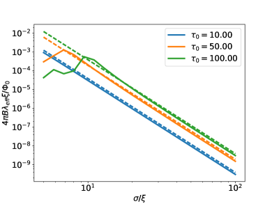
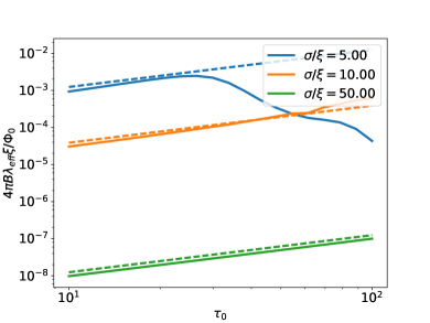
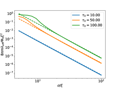
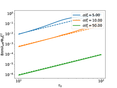
Figure 2: (Color online) The magnetic field in the center of the spot (a), (b) and the magnetic moment (c), (d) vs the beam size (a), (c) and intensity (b), (d). The solid line correspond to the solutions obtained numerically. The results of the adiabatic approximation for the weak field are represented by the dashed lines. The parameters of the Ginzburg–Landau functional are $\beta=1$ and $\zeta=0.5$, no screening is considered.

The magnetic field in the center of the spot and the magnetic moment of the currents versus the beam parameters $\sigma$ and $\tau_{0}$ are shown on the Fig. 2. The adiabatic approximation works reasonably for the slow temperature variations and fails if the local temperature is close to the critical one.

The dependence of the magnetic field in the center of the spot on the beam size $\sigma$ and the dimensionless power $\tau_{0}$ calculated for the Gaussian spot within the adiabatic approach (11) and numerically. The adiabatic approximation is reasonable for the slow temperature variations and fails if the local temperature is close to the critical temperature.

The maximal value of the field is reached when temperature in the center of the spot is close to the critical one. The field is given in the units of $H_{0}=\Phi_{0}/(4\pi\lambda_{\mathit{eff}}\xi)=H_{cm}/\sqrt{2}\cdot d/\lambda$ on the Fig. 2(a) and (b). The plot shows that the maximal field achieved for the small spots is between $10^{-2}\cdot H_{0}$ and $10^{-3}\cdot H_{0}$. At the border of applicability range we suppose that the thickness of the film is $d=\lambda$ and consider low temperature parameters $\xi=66$ nm and $\lambda=152$ nm. These assumptions give us an estimate of observable field up to $1.5$ G. In fact this value may be too optimistic due to the Meissner screening which comes into play for the thick enough samples.

The similar generation of the magnetic field in the hot spots may also occur in the other superconductors with the broken time reversal symmetry like $s+id$ superconductors Garaud et al. (2016). However the patterns of the magnetic field in the $s+id$ and the chiral $p$-wave superconductors appear to be qualitatively different due to the different symmetry of the superconducting states. Assuming an axially symmetric temperature distribution we find that the supercurrent and, thus, the magnetic field also has the axial symmetry. We neglected the terms in the free energy which reduce the symmetry of the superconductor to $D_{4h}$ so the pattern of the magnetic field is expected to have tetragonal distortions. This still qualitatively differs from the case of $s+id$ superconductor in which the pattern of the magnetic field has a pronounced two-fold symmetry Garaud et al. (2016). Thus, these types of pairing may be distinguished using the spatially resolved magnetic field measurements.

Another fingerprint of the chiral superconductivity is a nonzero magnetic moment of the thermally induced currents in the superconducting films. The key difference between the $s+id$ and $p_{x}+ip_{y}$ states is that the latter is characterized by an internal vorticity in the momentum space directed along the $z$ axis. Thus, in contrast to the $s+id$-wave superconductors the total magnetic moment of the induced currents (integrated over the sample) can be nonzero for a hot spot in a p-wave superconductor and the magnetic moment direction should depend on the internal vorticity which is proved by the above direct calculations. So magnetic moment measurements provide another possibility of provide of the chiral $p$-wave superconductivity.

IV Strong heating. Domain generation

In the case of the strong heating the temperature within the spot may exceed the critical temperature of the superconductor. This results in the significant suppression of the order parameter components. In this case one cannot apply the above perturbation approach directly however the qualitative picture is similar: there is a supercurrent flowing around the normal spot which creates magnetic field. However for a pulsed heat up the relaxation of temperature can cause the formation of the chiral domains according to the Kibble–Zurek mechanism Kibble (1976); H. Zurek (1985); Vadimov and Silaev (2013). The domain walls carry superconducting currentMatsumoto and Sigrist (1999) which can be detected by the techniques sensitive to the magnetic field. The same mechanism is responsible for creation of vortex–antivortex pairs in non-equilibrium transitions in $s$-wave superconductors Maniv et al. (2003) which can be identified by the specific magnetic field pattern. In the case of chiral $p$-wave superconductors the pattern of the magnetic field appears to reveal a number of specific features which can be used to distinguish this type of pairing.

We are using the approximation of the local temperature assuming now that it can depend on time. We start from the strongly non-homogeneous temperature distribution which gradually relaxes to the equilibrium value $T=T_{0}$. We studied the growth of the chiral domains numerically within the time-dependent Ginzburg–Landau approach:

$$-t_{\mathit{GL}}\left(\frac{\partial}{\partial t}+\frac{2\pi ic}{\Phi_{0}}\varphi\right)\eta_{+}=\chi_{+}(\mathbf{r},t)-\tau(\mathbf{r},t)\eta_{+}+\\ \eta_{+}|\eta_{+}|^{2}+\eta_{+}|\eta_{-}|^{2}(1+\beta)+\xi^{2}\left(\mathbf{D}^{2}\eta_{+}+2\zeta D_{+}^{2}\eta_{-}\right)\ ,\\$$ (18)

$$-t_{\mathit{GL}}\left(\frac{\partial}{\partial t}+\frac{2\pi ic}{\Phi_{0}}\varphi\right)\eta_{-}=\chi_{-}(\mathbf{r},t)-\tau(\mathbf{r},t)\eta_{-}+\\ \eta_{-}|\eta_{-}|^{2}+\eta_{-}|\eta_{+}|^{2}(1+\beta)+\xi^{2}\left(\mathbf{D}^{2}\eta_{-}+2\zeta D_{-}^{2}\eta_{+}\right)\ ,\\$$ (19)

$$\sigma_{n}\nabla^{2}\varphi+{c}\mathop{\mathrm{div}}\frac{\delta F}{\delta\mathbf{A}}=0\ ,$$ (20)

$$\frac{\sigma_{n}}{c}\frac{\partial\mathbf{A}}{\partial t}+\frac{c}{4\pi}\mathop{\mathrm{curl}}\mathop{\mathrm{curl}}\mathbf{A}+\sigma_{n}\nabla\varphi+c\frac{\delta F}{\delta\mathbf{A}}=0\ .$$ (21)

The Coulomb gauge $\mathop{\mathrm{div}}\mathbf{A}=0$ is considered, $\sigma_{n}$ is the normal state conductivity, $t_{GL}=\Gamma/a_{0}$ is the order parameter relaxation time and $\Gamma$ is a temperature independent constant. The functions $\chi_{\pm}$ are the delta–correlated noise sources $\langle\chi_{\alpha}(\mathbf{r},t)\chi_{\beta}(\mathbf{r}^{\prime},t^{\prime})\rangle=\chi^{2}\delta_{\alpha_{\beta}}\delta(\mathbf{r}-\mathbf{r}^{\prime})\delta(t-t^{\prime})$. Here we assume the thickness of the superconducting film to exceed the penetration length $\lambda$ but to be small enough so that the sample could be heated homogeneously in $z$ direction. These simplifications allow us to consider 2D Meissner screening instead of solving the full 3D problem. The heat equation was not taken into account selfconsistently. Instead the explicit model spatial and temporal profile of temperature was specified $\tau=1-\frac{\tau_{0}\xi^{2}}{\sigma^{2}}\exp\left(-r^{2}/[2\sigma^{2}]-t/t_{\mathit{T}}\right)$, where $t_{\mathit{T}}$ is the temperature relaxation time which is determined, e.g., by the heat flow into the substrate.

If the temperature quench is adiabatically slow ($t_{T}\ggg t_{GL}$) then the order parameter adiabatically follows the quasiequilibrium solution which is slightly disturbed by the thermal fluctuations. In this case the homogeneous domain appears after the quench is over. However if the temperature quench has the similar rate as the order parameter relaxation rate ($t_{T}\sim t_{GL}$) then the state of the superconductor is essentially non-equilibrium till the late stage of the quench. The nuclei of both order parameter components arise from the thermal fluctuations and grow rapidly until they are stabilized by the nonlinear terms in the Ginzburg–Landau equation. The order parameter relaxation time $t_{GL}$ diverges at the temperatures close to the critical one $t_{GL}\propto(T_{c}-T_{0})^{-1}$ so the domain nucleation is likely to occur in the vicinity of the phase transition.

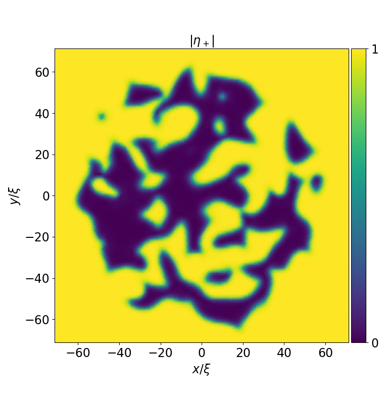
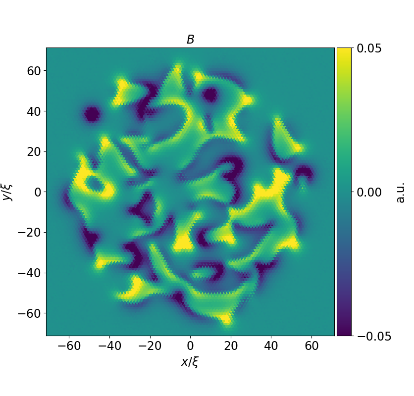
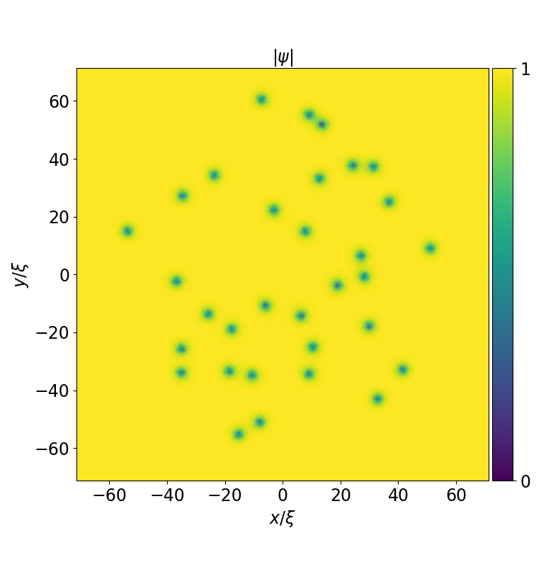
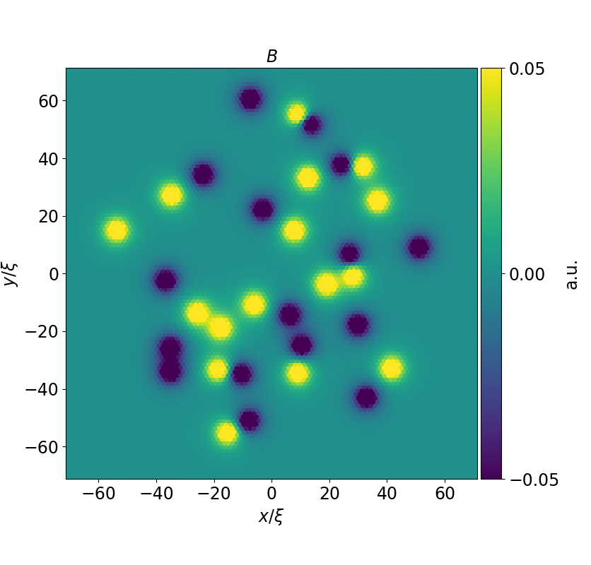
Figure 3: (Color online) The results of the Kibble–Zurek quench for a $p$-wave superconductor (a,b) and a $s$-wave superconductor described by a simple one–component Ginzburg–Landau model (c,d). (a,c) The absolute values of the superconducting order parameters. On the panel (a) only the component $\eta_{+}$ is shown (the component $\eta_{-}$ is dominant in the areas where $\eta_{+}$ is suppressed). (b,d) The pattern of the magnetic field within the sample after the quench. The magnetic field outside the film is expected to be partially smoothed out.

The results of the simulation are shown in the Fig. 3 (a,b). The peculiar picture of the chiral domains appears after a long time of simulation when the temperature is stabilized. The currents of the domain structure generate the inhomogeneous magnetic field pattern with the zero total flux. The distribution of the magnetic field qualitatively differs from the case of conventional $s$-wave superconductor for which Kibble–Zurek mechanism is known to be responsible for generation of vortex–antivortex pairsManiv et al. (2003) (see Fig. 3 (c,d)). One can expect that the generation of the domain structure should be accompanied by the generation of the vortex–antivortex pairs in the bulk of the domains but most of the vortices appear to be pinned at the domain walls. The pinned vortices can be found in the Fig. 3(b) as asymmetric peaks of magnetic field. At the early stage of the Kibble-Zurek quench both the vortices and the domain walls nucleate but eventually the vortices move to the domain walls and remain trapped there. Thus, amount of unpinned vortices depends on the vortex–domain wall interaction strength.

The same reasoning is valid for any multicomponent superconductor which supports the formation of the domain walls like $s+id$ superconductors. In this case a similar magnetic field pattern which corresponds to the system of domain walls with the vortices pinned at the walls is expected after the Kibble–Zurek quench which complicates identification of the chiral $p$-wave superconductivity in the sample. However as we noted in the Section III the magnetic moment of the currents in the films of the non-chiral superconductors vanishes so it it possible to distinguish these types of pairing performing the measurement of the magnetic moment of the sample after the quench.

V Domain stability

The vortex–antivortex pairs which appear in the conventional superconductors according to the Kibble–Zurek scenario are unstable due to the attraction between the vortices of the opposite winding numbers. However the impurities in the sample can pin the vortices thus preventing the relaxation to the homogeneous state. The similar scenario may be relevant for the domains in the chiral superconductor: the domains can be unstable and shrink eventually, so the domain picture can be observed only within a finite time after the quench unless we take pinning into account. Though the total vorticity of the dominating order parameter component is equal to zero the winding number around some domains may be nonzero affecting the evolution of the domain. We are going to discuss the dynamics of the domains using an extension of the London theory for the chiral $p$-wave superconductor assuming $\lambda/\xi\gg 1$.

We restrict ourselves to the 2D case so the domain walls are the contours which separate the domains of different chirality. The absolute values of the order parameter components in the bulk of the domain are (1,0) or (0, 1) depending on the domain type so we can consider the phase of the dominant order parameter component as a dynamic variable within the corresponding domains. This gives us the usual expression for the free energy of the bulk of the domains:

$$F_{\mathit{bulk}}=\frac{\Phi_{0}^{2}}{32\pi^{3}\lambda_{\mathit{eff}}}\sum\limits_{\alpha=+,-}\int\limits_{\Omega_{\alpha}}\left(\nabla\theta_{\alpha}-\frac{2\pi}{\Phi_{0}}\mathbf{A}\right)^{2}\;d^{2}r,$$ (22)

where $\theta_{\pm}$ are the phases of the order parameter components and $\Omega_{\pm}$ are the areas occupied by the chiral domains. The domain wall can be viewed as a Josephson junction between the domains with a certain equilibrium superconducting phase difference. The optimal phase difference though depends on the wall orientation as $\theta_{+}-\theta_{-}=2\theta_{n}$ for the flat equilibrium walls where $\theta_{n}$ is the angle between the normal direction to the wall and the crystal axisSigrist and Agterberg (1999) in the abscence of tetragonal distortions. Assuming the curvature of the wall to be much less than $\xi^{-1}$ one can consider the wall to be almost flat at each point and write the free energy of the domain wall as follows:

$$F_{\mathit{wall}}=\frac{\Phi_{0}^{2}}{32\pi^{3}\lambda_{\mathit{eff}}}\oint\limits_{\mathit{DW}}\left\{\epsilon+j\cos\left(\theta_{+}-\theta_{+}-2\theta_{n}\right)\right\}\;dl\ ,$$ (23)

where the integration is taken over all domain walls, $\epsilon$ and $j$ are the positive constants which characterize the energy of the domain wall and the Josephson energy per unit length, respectively. The domain walls are energetically unfavorable so the condition $\epsilon>j$ must be satisfied. The energy of the wall can be obtained straightforwardly from the Ginzburg–Landau functional by integrating the free energy density over the short segment across the wall, assuming step–like form of the absolute values of the order parameter components. Using this approach one can estimate the parameters $\epsilon\propto\xi^{-1}$ and $j\propto\zeta\xi^{-1}$, respectively, and find the additional corrections to the wall energy which come from the phase gradients at the sides of the wall. These corrections allow to take account of the supercurrents flowing along the wall Sigrist and Agterberg (1999) which cannot be described within the simple Josephson–like model. However in the case of strong type-II superconductor $\lambda/\xi\gg 1$ and weak interaction between the order parameter components $\zeta\ll 1$ the Josephson–like term gives the most significant contribution into the energy of the domain wall. The free energy of the sample naturally comes as a sum of bulk and interface terms:

$$F=F_{\mathit{wall}}+F_{\mathit{bulk}}\ .$$ (24)

This functional yields Laplace equations for the both phases of the order parameter components with the nonlinear boundary conditions at the domain walls:

$$\nabla^{2}\theta_{\pm}=0\ ,$$ (25)

$$\left.\frac{\partial\theta_{\pm}}{\partial n}-j\sin\left(\theta_{+}-\theta_{-}-2\theta_{n}\right)\right|_{\mathit{DW}}=0.$$ (26)

Here $n$ stands for direction normal to the domain wall from the “plus” to the “minus” domains.

Using the above model we study the stability of a circular domain of radius $R$ which carries no magnetic flux. This requires the abscence of vorticity in the exterior domain (for certainty we consider $\eta_{+}$ domain to be an exterior one), i.e. the phase of the corresponding order parameter component must be a single-valued function. We neglect the vector potential $\mathbf{A}$ assuming the sample to be a thin film and the domain size $R$ to be much less than the effective penetration length $\lambda_{\mathit{eff}}$. Due to the nonlinearity of the boundary conditions (26) the exact solution of the equations (25) appears to be complicated. However in the case of the small domains and weak interaction between the order parameter components so $jR\ll 1$ one can linearize the boundary conditions. We suppose that the phases are almost constant, i.e. $|\theta_{\pm}(\mathbf{r})-\Theta_{\pm}|\ll 1$ for some $\Theta_{\pm}=const$. Due to the gauge invariance an arbitrary constant may be added to both $\Theta_{+}$ and $\Theta_{-}$ while change of the difference $\Theta_{+}-\Theta_{-}$ results in rotation of the whole domain. Thus without a loss of generality we can assume $\Theta_{+}=\Theta_{-}=0$. The phases $\theta_{\pm}$ must satisfy the Laplace equation with the following boundaries:

$$\frac{\partial\theta_{+}}{\partial r}=j\sin 2\varphi\ ,$$ (27)

$$\frac{\partial\theta_{-}}{\partial r}=j\sin 2\varphi\ .$$ (28)

Here the angle $\theta_{n}$ which determines the direction of the normal simply coincides with the polar angle $\varphi$. One can easily find the solutions

$$\theta_{\pm}=\mp\frac{jR}{2}\left(\frac{r}{R}\right)^{\mp 2}\sin 2\varphi$$ (29)

and obtain the free energy of the domain in the lowest order by $R$:

$$F\approx 2\pi R\epsilon\ .$$ (30)

The minimum is at $R=0$ which means than the small domains cannot be stable.

The solution (29) of the equation (25) for the small domains can be used as an appropriate ansatz for the nonlinear problem which appears if the domain is large $jR\gg 1$. We look for the solution in form of the trial function:

$$\theta_{\pm}=\gamma_{\pm}\left(\frac{r}{R}\right)^{\pm 2}\sin 2\varphi\ ,$$ (31)

where $\gamma_{\pm}$ are unknown parameters and substitute it into the free energy (24):

$$F=2\pi\left[\gamma_{+}^{2}+\gamma_{-}^{2}+R\varepsilon+jRJ_{1}(\gamma_{+}-\gamma_{-})\right]\ .$$ (32)

If $jR\gg 1$ the minimum is $\gamma_{\pm}=\mp x_{0}/2$ where $x_{0}\approx 1.84$ is the position of the first maximum of the Bessel function $J_{1}(x)$. The final expression for the free energy is

$$F\approx 2\pi R\left[\epsilon-jJ_{1}(x_{0})\right]$$ (33)

The dependence also appears to be linear and $dF/dR>0$ so the domain cannot be stabilized though the slope of the curve $F(R)$ is reduced compared to the case of the small domain.

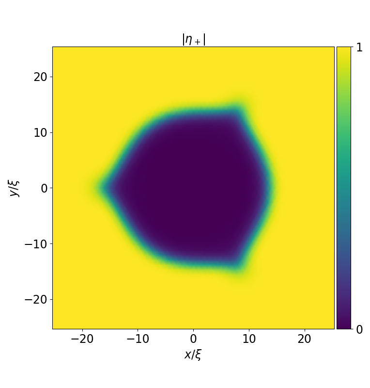
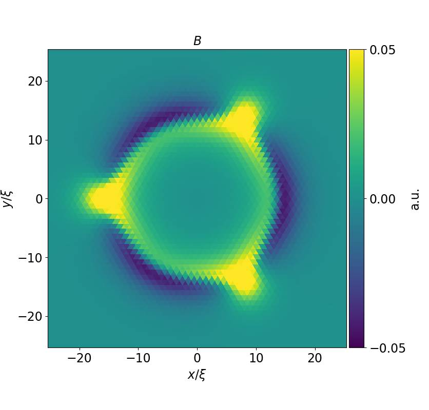
Figure 4: (Color online) The order parameter (a) and the magnetic field (b) of the chiral domain with three vortices pinned by the domain wall. The winding number of the outer order parameter component $\eta_{+}$ is equal to -1. The vortices reveal themself as localized peaks of magnetic field. The domain shown on the figure is not stable configuration but a snapshot of the domain evolution.

However the circular domain can be stabilized if it carries two quanta of magnetic flux. The order parameter of the exterior domain thus has vorticity equal to $\pm 2$ depending on the domain type. In our case $\theta_{-}=\pi$ and $\theta_{+}=2\varphi$. This solution satisfies Laplace equation inside the domains and the boundary conditions at the domain wall because it minimizes the Josephson–like energy along the whole wall. The free energy of such domain is given by the following expression:

$$F=\frac{\Phi_{0}^{2}}{16\pi^{2}\lambda_{\mathit{eff}}}\left[4\ln\frac{\lambda_{\mathit{eff}}}{R}+(\epsilon-j)R\right]\ .$$ (34)

The free energy of the exterior domain diverges logarithmically at $r\to\infty$ so the integral was cutted off at $r=\lambda_{\mathit{eff}}$. The free energy has a local minimum at $R_{\ast}=4/(\epsilon-j)$, i.e. the domain carrying two quanta of the magnetic flux is stable to the radial perturbations. The numerical simulations performed within the time dependent Ginzburg–Landau framework show stability of the two–quanta domains with respect to the azimuthal perturbations.

The above model may be applied for arbitrary vorticity $n$ of the exterior order parameter. The presence of nonzero vorticity leads to the logarithmic term $\propto n^{2}\ln(\lambda_{\mathit{eff}}/R)$ in the free energy expression which comes from the kinetic energy of the Cooper pairs in the exterior domain. This term stabilizes the domain at some finite radius. However in this model all the domains are considered to be circular which is not true if $n\neq\pm 2$. The Josephson energy is frustrated in this case and such domains lose circularity due to the azimuthal instability.

This instability reveals itself in appearance of the vortices pinned by the domain wall. These vortices represent the short segments of the wall where the phases of the order parameter components are inconsistent with the Josephson relation. Between these vortices the Josephson–like energy of the domain wall is minimized. The simulations performed within the time dependent Ginzburg–Landau model show that these vortices lead to the sharp bending of the domain wall and loss of the cylindrical symmetry of the domain (see Fig. 4). The azimuthal instability plays crucial role in the evolution of the domains allowing the domains with $n\neq 0$ to shrink.

VI Summary

In this work we have studied the effect of the laser pulse on the film of a chiral superconductor. Reducing the influence of the laser pulse to the only effect of the sample heating we have found the distribution of the order parameter components and the magnetic field within the hot spot. We have analyzed the dynamics of the superconductor after the pulse absorption in the regime of a subsequent temperature quench. We show that if the initial pulse was strong enough to suppress superconductivity locally then the chiral domains may grow during the temperature quench according to the Kibble–Zurek scenario. The magnetic field created by the currents of the domain walls can be observed experimentally. The field pattern of the domain walls differs qualitatively from the field of vortex–antivortex pairs known to appear via Kibble–Zurek mechanism in the conventional $s$-wave superconductors. Such a behavior is a fingerprint of the chiral superconductivity and the appropriate experiments may be useful for it’s identification in $\mathrm{Sr_{2}RuO_{4}}$.

In order to study the stability of the domains we developed a model which allows to analyze the samples with the given shape of the domains in London limit assuming the domain wall to be a Josephson junction with orientation–dependent Josephson energy. Using this model we studied stability of the circular domains and show that two–quanta domains are stable while zero–quanta domains shrink. Simulations within the time dependent Ginzburg–Landau framework show that the circular domains are unstable with respect to the azimuthal perturbations if the winding number of the exterior domain differs from $\pm 2$ due to the Josephson energy frustration similar to the frustration in the circular Josephson junctions between the chiral $p$-wave and the $s$-wave superconductors Etter et al. (2014).

We thank I. Shereshevskii, D. Vodolazov, A. Buzdin, Ph. Tamarat and B. Lounis for stimulating discussions. The work was supported by Russian Science Foundation No. 17-12-01383 (ASM), Foundation for the advancement of theoretical physics “BASIS” No. 109 (VLV) and Russian Foundation for Basic Research (VLV).

References

- Kirilyuk et al. (2013) A. Kirilyuk, A. V. Kimel, and T. Rasing, Reports on Progress in Physics 76, 026501 (2013).
- Kirilyuk et al. (2010) A. Kirilyuk, A. V. Kimel, and T. Rasing, Rev. Mod. Phys. 82, 2731 (2010).
- Fausti et al. (2011) D. Fausti, R. Tobey, N. Dean, S. Kaiser, A. Dienst, M. C. Hoffmann, S. Pyon, T. Takayama, H. Takagi, and A. Cavalleri, Science 331, 189 (2011).
- Suda et al. (2015) M. Suda, R. Kato, and H. M. Yamamoto, Science 347, 743 (2015).
- Veshchunov et al. (2016) I. S. Veshchunov, W. Magrini, S. Mironov, A. Godin, J.-B. Trebbia, A. I. Buzdin, P. Tamarat, and B. Lounis, Nature communications 7, 12801 (2016).
- Yuzbashyan et al. (2006) E. A. Yuzbashyan, O. Tsyplyatyev, and B. L. Altshuler, Phys. Rev. Lett. 96, 097005 (2006).
- Matsunaga et al. (2014) R. Matsunaga, N. Tsuji, H. Fujita, A. Sugioka, K. Makise, Y. Uzawa, H. Terai, Z. Wang, H. Aoki, and R. Shimano, Science 345, 1145 (2014).
- Semenov et al. (2001) A. D. Semenov, G. N. Gol’tsman, and A. A. Korneev, Physica C: Superconductivity 351, 349 (2001).
- Gol’tsman et al. (2001) G. N. Gol’tsman, O. Okunev, G. Chulkova, A. Lipatov, A. Semenov, K. Smirnov, B. Voronov, A. Dzardanov, C. Williams, and R. Sobolewski, Applied Physics Letters 79, 705 (2001).
- Maingault et al. (2010) L. Maingault, M. Tarkhov, I. Florya, A. Semenov, R. E. de Lamaëstre, P. Cavalier, G. Gol’tsman, J.-P. Poizat, and J.-C. Villégier, Journal of Applied Physics 107, 116103 (2010).
- Zotova and Vodolazov (2012) A. N. Zotova and D. Y. Vodolazov, Phys. Rev. B 85, 024509 (2012).
- Kibble (1976) T. W. B. Kibble, Journal of Physics A: Mathematical and General 9, 1387 (1976).
- H. Zurek (1985) W. H. Zurek, Nature, 317, 505 (1985).
- Volovik (2000) G. E. Volovik, Physica B 280, 122 (2000).
- Maniv et al. (2003) A. Maniv, E. Polturak, and G. Koren, Phys. Rev. Lett. 91, 197001 (2003).
- Note (1) The projections of the angular momentum are bad quantum numbers in the crystals due to the lack of continuous rotational symmetry. The true structure of the gap is described by the basis functions of some irreducible representation of the crystal symmetry group which corresponds to the certain superconducting state. Still these functions can be classified by the average value of the angular momentum.
- Volovik and Mineev (1981) G. Volovik and V. Mineev, Zh. Eksp. Teor. Fiz 81, 989 (1981).
- Volovik (1975) G. Volovik, JETP LETTERS 22, 108 (1975).
- Cross (1975) M. C. Cross, Journal of Low Temperature Physics 21, 525 (1975).
- Sauls (2011) J. A. Sauls, Phys. Rev. B 84, 214509 (2011).
- Lederer et al. (2014) S. Lederer, W. Huang, E. Taylor, S. Raghu, and C. Kallin, Phys. Rev. B 90, 134521 (2014).
- Huang et al. (2015) W. Huang, S. Lederer, E. Taylor, and C. Kallin, Phys. Rev. B 91, 094507 (2015).
- Bakurskiy et al. (2017) S. V. Bakurskiy, N. V. Klenov, I. I. Soloviev, M. Y. Kupriyanov, and A. A. Golubov, Superconductor Science and Technology 30, 044005 (2017).
- Kirtley et al. (2007) J. R. Kirtley, C. Kallin, C. W. Hicks, E.-A. Kim, Y. Liu, K. A. Moler, Y. Maeno, and K. D. Nelson, Phys. Rev. B 76, 014526 (2007).
- Kallin (2012) C. Kallin, Rep. Prog. Phys. 75, 042501 (2012).
- Scaffidi and Simon (2015) T. Scaffidi and S. H. Simon, Phys. Rev. Lett. 115, 087003 (2015).
- Huang et al. (2014) W. Huang, E. Taylor, and C. Kallin, Phys. Rev. B 90, 224519 (2014).
- Tada et al. (2015) Y. Tada, W. Nie, and M. Oshikawa, Phys. Rev. Lett. 114, 195301 (2015).
- Volovik (2014) G. E. Volovik, cond-mat arXiv:1409.8638 (2014).
- Bouhon and Sigrist (2014) A. Bouhon and M. Sigrist, Phys. Rev. B 90, 220511 (2014).
- Imai et al. (2013) Y. Imai, K. Wakabayashi, and M. Sigrist, Phys. Rev. B 88, 144503 (2013).
- Garaud et al. (2016) J. Garaud, M. Silaev, and E. Babaev, Phys. Rev. Lett. 116, 097002 (2016).
- Heeb and Agterberg (1999) R. Heeb and F. D. Agterberg, Phys. Rev. B 59, 7076 (1999).
- Barash and Mel’nikov (1991) Y. S. Barash and A. S. Mel’nikov, JETP 100, 307 (1991).
- Vadimov and Silaev (2013) V. Vadimov and M. Silaev, Phys. Rev. Lett. 111, 177001 (2013).
- Balatskii and Mineev (1985) A. V. Balatskii and V. P. Mineev, Zh. Teor. Eksp. Fiz. 89, 2073 (1985).
- Gulyan and Zharkov (1985) A. Gulyan and G. Zharkov, JETP 62, 89 (1985).
- Matsumoto and Sigrist (1999) M. Matsumoto and M. Sigrist, Journal of the Physical Society of Japan 68, 994 (1999).
- Sigrist and Agterberg (1999) M. Sigrist and D. Agterberg, Progress of Theoretical Physics 102, 965 (1999).
- Etter et al. (2014) S. B. Etter, H. Kaneyasu, M. Ossadnik, and M. Sigrist, Phys. Rev. B 90, 024515 (2014).