Computing mean logarithmic mass from muon counts in air shower experiments

Abstract

I discuss the conversion of muon counts in air showers, which are observable by experiments, into mean logarithmic mass, an important variable to express the mass composition of cosmic rays. Stochastic fluctuations in the shower development and statistical fluctuations from muon sampling can subtly bias the conversion. A central theme is that the mean of the logarithm of the muon number is not identical to the logarithm of the mean. It is discussed how that affects the conversion in practice. Simple analytical formulas to quantify and correct such biases are presented, which are applicable to any kind of experiment.

I Introduction

The mean logarithmic mass $\langle{\ln A}\rangle$ is a common variable to summarize the mass composition of cosmic rays. Most ground-based experiments infer the mass by counting muons in cosmic-ray induced air showers Kampert and Unger (2012). This paper discusses the conversion of muon number to mean logarithmic mass from the point of view of the data analyst, with a focus on the effect of stochastic fluctuations in the shower development and the detector response on the conversion. The fluctuations can bias estimates of $\langle{\ln A}\rangle$ in several ways. Biases here are defined in the usual statistical sense; if $\hat{x}$ is an estimate of the true value $x$ that fluctuates according to a probability density $f(\hat{x})$, then the bias is the expectation $\operatorname{E}[\hat{x}-x]=\int(\hat{x}-x)f(\hat{x})\text{d}\hat{x}$. We generally want $\hat{x}$ to have zero bias, so that the sample average $\langle{\hat{x}}\rangle$ converges to $x$ for large samples.

The results in this paper are not specific to a particular type of experiment. It is assumed throughout this paper that an experiment provides an unbiased estimate $\hat{N}_{\mu}$ of the total number of muons $N_{\mu}$ produced in an air shower and an estimate $\hat{E}$ of the shower energy $E$. This is far from trivial and much of the difficulty in running an experiment deals with this. The total number of muons $N_{\mu}$ produced in an air shower cannot be directly measured, because experiments can only count muons that reach the ground, while some decay on the way. The experimental distinction between muons and other charged particles at the ground is not easy either Aab et al. (2014); Abbasi et al. (2013); Apel et al. (2015); Abu-Zayyad et al. (2000). But in principle, $\hat{N}_{\mu}$ can be inferred for a given geometry and shower energy from the measurement by applying an average correction obtained from air shower simulations. Highly-inclined air showers recorded by Haverah Park and the Pierre Auger Observatory have been analyzed in this way Ave et al. (2000a, b); Dembinski et al. (2010); Aab et al. (2015). Similarly, an estimate $\hat{E}$ of the shower energy can be inferred from the number of electrons and photons that reach the ground, or by recording the longitudinal shower profile with telescopes.

The paper deals with the comparably easier part of the conversion of the unbiased estimates $\hat{E},\hat{N}_{\mu}$ to $\langle{\ln A}\rangle$. Fluctuations occur in the shower development and arise from the sampling of an air shower by a detector. It is important to distinguish between these two kinds of fluctuations, because they are approximately independent Dembinski et al. (2016). Both randomly shift the estimates $\hat{E},\hat{N}_{\mu}$ away from their true values $E,N_{\mu}$, and these random shifts cause some subtle biases in the conversion to $\langle{\ln A}\rangle$. We quantify these biases. Knowing their sizes allows one to safely neglected them if they are small, and to correct them otherwise.

II From muon number to mass

It is instructive to introduce fluctuations step-by-step. We start by ignoring fluctuations from detector sampling and consider only stochastic fluctuations in the shower development. The true muon number $N_{\mu}$ and the shower energy $E$ shall be exactly known and the energy $E$ shall be same for all showers. Stochastic fluctuations in the hadronic interactions are still causing the muon number $N_{\mu}$ to vary randomly.

The first point to make is that $\langle{\ln A}\rangle$ is best computed from the mean logarithmic muon number $\langle{\ln N_{\mu}}\rangle$, and not the mean of the muon number $\langle{N_{\mu}}\rangle$. In either case, the average here is computed over many air showers with the same shower energy $E$.

The following argument is similar to the one developed by the Pierre Auger collaboration for the depth of shower maximum Abreu et al. (2013). The relationship between $N_{\mu}$ and $A$ can be understood within the Matthews-Heitler model of a hadronic shower Matthews (2005). The analytical model treats air showers in a simplified way, but describes surprisingly many features of air showers correctly. According to the model, the total muon number $N_{\mu}$ for a cosmic ray with $A$ nucleons scales with a power of the number of nucleons

$$N_{\mu}=A^{1-\beta}\,N_{\mu}^{p},$$ (1)

where $N_{\mu}^{p}$ is the number of muons in a proton-induced air shower, and $\beta\simeq 0.9$ is a constant.

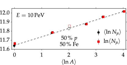
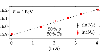
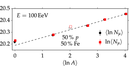
Figure 1: Average logarithm of the number of muons $\langle{\ln N_{\mu}}\rangle$ (circles) and logarithm of the average number of muons $\ln\langle{N_{\mu}}\rangle$ (squares) in simulated vertical air showers produced by primary particles with $A$ nucleons. A fitted straight line (dashed) is shown for comparison. Solid markers stand for averages computed over showers from a single primary, open markers stand for an equal mix of proton and iron showers. Error bars indicate the statistical uncertainty of the finite sample (2200 showers per primary and energy).

This behavior is well reproduced in full air shower simulations. In the Matthews-Heitler model, stochastic fluctuations in the shower development are neglected. To show that Eq. 1 holds for the real showers, several sets of vertical showers with identical primary particles were simulated with CORSIKA Heck et al. (1998) compiled with the CONEX option, using the hadronic interaction models SIBYLL-2.3 Riehn et al. (2015) and GHEISHA Fesefeldt (1985). The showers were simulated in a US standard atmosphere until a slant depth of $1050\text{\,}\mathrm{g}\mathrm{c}\mathrm{m}^{-2}$. The number of muons $N_{\mu}$ in each shower were taken from the maximum of the longitudinal muon profile. Proton, helium, nitrogen, silicon, and iron primaries were simulated. For each primary, the averages $\ln\langle{N_{\mu}}\rangle$ and $\langle{\ln N_{\mu}}\rangle$ were computed. The two are subtly different, because the expectation is noncommutative with a non-linear mapping $f(x)$, $\operatorname{E}[f(x)]\neq f(\operatorname{E}[x])$. The dependence on $A$ is shown in Fig. 1 for a wide range of primary energies. For a pure composition where all showers are initated by a primary with the same mass $A$, both $\ln\langle{N_{\mu}}\rangle$ and $\langle{\ln N_{\mu}}\rangle$ scale with $\ln A$ as predicted by Eq. 1. This result is independent of the hadronic interaction model and shower inclination.

To use Eq. 1 to get an estimate of $\langle{\ln A}\rangle$ for real air showers, we consider the realistic case where the mass $A$ is another stochastic variable that changes from shower to shower. For a pure composition, the simulations showed that $\langle{N_{\mu}}\rangle=A^{1-\beta}\,\langle{N_{\mu}^{p}}\rangle$ . If $f_{A}$ is the fraction of primaries with $A$ nucleons in a mixed composition, we have

$$\begin{gathered}\sum_{A}f_{A}\langle{N_{\mu}}\rangle=\sum_{A}f_{A}\,A^{1-\beta}\,\langle{N_{\mu}^{p}}\rangle=\langle{N_{\mu}^{p}}\rangle\sum_{A}f_{A}\,A^{1-\beta}\\ \Leftrightarrow\quad\langle{N_{\mu}}\rangle=\langle{N_{\mu}^{p}}\rangle\,\langle{A^{1-\beta}}\rangle.\end{gathered}$$ (2)

Unfortunately, we cannot convert $\langle{A^{1-\beta}}\rangle$ to $\langle{A}\rangle$ or $\langle{\ln A}\rangle$, because these are non-linear functions of $A$. The solution is to start from $\langle{\ln N_{\mu}}\rangle=(1-\beta)\ln A+\langle{\ln N_{\mu}^{p}}\rangle$ for a pure composition, which is also supported by the simulations. Then the result of the superposition is

$$\langle{\ln N_{\mu}}\rangle=(1-\beta)\langle{\ln A}\rangle+\langle{\ln N_{\mu}^{p}}\rangle,$$ (3)

where we used that $\langle{ax+by}\rangle=a\langle{x}\rangle+b\langle{y}\rangle$ for constants $a,b$ and stochastic variables $x,y$.

Both $\beta$ and $\langle{\ln N_{\mu}^{p}}\rangle$ can be obtained from air shower simulations. If $\langle{\ln N_{\mu}^{\text{Fe}}}\rangle$ is available, it can be used to substitute $\beta$. The two related formulas for $\langle{\ln A}\rangle$ are

$$\langle{\ln A}\rangle =\frac{\langle{\ln N_{\mu}}\rangle-\langle{\ln N_{\mu}^{p}}\rangle}{1-\beta}$$ (4)

$$\langle{\ln A}\rangle =\frac{\langle{\ln N_{\mu}}\rangle-\langle{\ln N_{\mu}^{p}}\rangle}{\langle{\ln N_{\mu}^{\text{Fe}}}\rangle-\langle{\ln N_{\mu}^{p}}\rangle}\ln 56.$$ (5)

This approach is very elegant, because the equations are true whatever the probability distributions are for $A$, $N_{\mu}$, $N_{\mu}^{p}$, and $N_{\mu}^{\text{Fe}}$.

As previously stated, the mean of the logarithm is not the same as the logarithm of the mean, $\ln\langle{N_{\mu}}\rangle$ is always higher than $\langle{\ln N_{\mu}}\rangle$. Still, the two are quite close and the bias of substituting one for the other may be negligible in some situations. To judge when this is safe, a simple formula to compute the bias is given in section III. Some analyses Dembinski and Gonzalez (2016) do not produce an estimate of the muon number event-by-event, only the average $\langle{N_{\mu}}\rangle$ over many showers. In these cases, the formula can be used to correct the difference $(\langle{\ln N_{\mu}}\rangle-\ln\langle{N_{\mu}}\rangle)$.

So far fluctuations introduced by detector sampling were neglected, but $N_{\mu}$ is not known in practice, only an estimate $\hat{N}_{\mu}$ which fluctuates around $N_{\mu}$. Some muons decay on the way to the ground, the detector does not count all muons that arrive, and so on. It is assumed that these losses are corrected on average, but they introduces additional fluctuations. Since the mean of the logarithm is not the logarithm of the mean, we find $\langle{\ln\hat{N}_{\mu}}\rangle\neq\langle{\ln N_{\mu}}\rangle$ even if $\hat{N}_{\mu}$ is an unbiased estimate of $N_{\mu}$. How to correct for this effect is discussed in section IV.

Finally, one has to consider that the average $\langle{\ln\hat{N}_{\mu}}\rangle$ is not computed over showers with the same energy $E$ in practice, but for showers that fall into the same energy bin. The energy $E$ is also not known exactly, only an estimate $\hat{E}$ of it. The quantitative impact of that is calculated in section V.

III Muon number: Mean logarithm and logarithm of mean

The difference $(\langle{\ln N_{\mu}}\rangle-\ln\langle{N_{\mu}}\rangle)$ can be calculated with a simple formula. To derive it, we use the following general substitution

$$N_{\mu}=\langle N_{\mu}\rangle(1+\epsilon),$$ (6)

where $\epsilon=(N_{\mu}-\langle N_{\mu}\rangle)/\langle N_{\mu}\rangle$ is the relative random deviation of the muon number from its mean. By construction, $\langle\epsilon\rangle=0$. The average logarithmic muon number is

$$\langle\ln N_{\mu}\rangle =\langle\ln[\langle N_{\mu}\rangle(1+\epsilon)]\rangle$$

$$=\ln\langle N_{\mu}\rangle+\langle\ln(1+\epsilon)\rangle.$$ (7)

For small relative fluctuations, $\epsilon\ll 1$, the second logarithm can be expanded into a Taylor series,

$$\langle\ln N_{\mu}\rangle =\ln\langle N_{\mu}\rangle+\langle\epsilon-\frac{1}{2}\epsilon^{2}+\mathcal{O}(\epsilon^{3})\rangle$$

$$=\ln\langle N_{\mu}\rangle-\frac{1}{2}\langle\epsilon^{2}\rangle+\langle\mathcal{O}(\epsilon^{3})\rangle.$$ (8)

The second-order term $\langle{\epsilon^{2}}\rangle$ is equal to the variance of the relative deviations from the mean,

$$\langle{\epsilon^{2}}\rangle =\langle{\epsilon^{2}}\rangle-\langle{\epsilon}\rangle^{2}=\operatorname{Var}[\epsilon]$$

$$=\operatorname{Var}[(N_{\mu}-\langle N_{\mu}\rangle)/\langle N_{\mu}\rangle]=\operatorname{Var}[N_{\mu}]/\langle N_{\mu}\rangle^{2}.$$ (9)

Therefore, the offset can be computed for $\epsilon\ll 1$ as

$$\langle{\ln N_{\mu}}\rangle-\ln\langle{N_{\mu}}\rangle\approx-\frac{1}{2}\operatorname{Var}[(N_{\mu}-\langle N_{\mu}\rangle)/\langle N_{\mu}\rangle].$$ (10)

$E/\mathrm{eV}$	$10^{15}$	$10^{16}$	$10^{17}$	$10^{18}$	$10^{19}$	$10^{20}$
	p
$\langle\ln N_{\mu}\rangle$	$9.55$	$11.64$	$13.73$	$15.89$	$18.01$	$20.22$
$\ln\langle N_{\mu}\rangle$	$9.58$	$11.66$	$13.76$	$15.91$	$18.02$	$20.23$
$\mathrm{Var}[\epsilon]$	$0.051$	$0.038$	$0.038$	$0.022$	$0.030$	$0.017$
	He
$\langle\ln N_{\mu}\rangle$	$9.66$	$11.78$	$13.890$	$15.99$	$18.143$	$20.276$
$\ln\langle N_{\mu}\rangle$	$9.67$	$11.787$	$13.894$	$16.00$	$18.145$	$20.279$
$\mathrm{Var}[\epsilon]$	$0.015$	$0.010$	$0.008$	$0.011$	$0.0049$	$0.0057$
	N
$\langle\ln N_{\mu}\rangle$	$9.783$	$11.877$	$13.992$	$16.105$	$18.221$	$20.355$
$\ln\langle N_{\mu}\rangle$	$9.787$	$11.879$	$13.994$	$16.107$	$18.222$	$20.356$
$\mathrm{Var}[\epsilon]$	$0.008$	$0.0042$	$0.0035$	$0.0027$	$0.0027$	$0.0019$
	Si
$\langle\ln N_{\mu}\rangle$	$9.887$	$11.957$	$14.048$	$16.159$	$18.274$	$20.407$
$\ln\langle N_{\mu}\rangle$	$9.891$	$11.959$	$14.049$	$16.160$	$18.275$	$20.407$
$\mathrm{Var}[\epsilon]$	$0.0067$	$0.0029$	$0.0021$	$0.0015$	$0.0012$	$0.0010$
	Fe
$\langle\ln N_{\mu}\rangle$	$9.947$	$12.017$	$14.109$	$16.212$	$18.330$	$20.454$
$\ln\langle N_{\mu}\rangle$	$9.950$	$12.018$	$14.109$	$16.213$	$18.331$	$20.455$
$\mathrm{Var}[\epsilon]$	$0.0044$	$0.0016$	$0.0016$	$0.0010$	$0.00049$	$0.00058$

Table 1: Simulation results for vertical showers simulated with hadronic models SIBYLL2.3 and GHEISHA, as described in section II. The total number of muons $N_{\mu}$ is taken from the maximum of the longitudinal muon profile.

Table 1 lists $\langle{\ln N_{\mu}}\rangle$, $\ln\langle{N_{\mu}}\rangle$, and $\operatorname{Var}[(N_{\mu}-\langle N_{\mu}\rangle)/\langle N_{\mu}\rangle]$ for the air shower simulations described in the previous section. A useful empirical parametrization of the latter is shown in the appendix. The numbers confirm for single elements that $\operatorname{Var}[\epsilon]\ll 1$, which implies $\epsilon\ll 1$. Eq. 10 is therefore a good approximation for single primaries above $10^{15}\,$\mathrm{e}\mathrm{V}$$.

It also holds for any mix of primaries. The variance for a mix of primaries is larger than for a single primary, because the difference in the means $\langle N_{\mu}\rangle$ of different primaries contributes to the variance. With the data in Table 1, $\operatorname{Var}[\epsilon]$ was computed for all pairs of primaries. The largest value $\operatorname{Var}[\epsilon]=0.063$ is found at $10^{15}\,$\mathrm{e}\mathrm{V}$$ for a mix of proton and iron. This value is still small and thus Eq. 10 remains valid.

With these numbers, it is possible to address the question whether using $\ln\langle{N_{\mu}}\rangle$ instead of $\langle{\ln N_{\mu}}\rangle$ in Eq. 4 or 5 introduces a noticeable bias. In the most extreme case, the bias is $(\ln\langle{N_{\mu}}\rangle-\langle{\ln N_{\mu}}\rangle)\approx 0.03$. In the conversion to $\langle{\ln A}\rangle$, this bias is multiplied by a factor $1/(1-\beta)$, see Eq. 4. For $\beta\simeq 0.9$, this is a factor of 10, so that the bias in $\langle{\ln A}\rangle$ is $0.3$. This is about 7 % of the overall difference between proton and iron. Using the wrong mean makes the composition appear heavier than it truly is. The effect is small, but since the bias is easy to correct with Eq. 10, applying the correction is recommended.

IV Bias from sampling fluctuations

The second type of difficulty in applying Eq. 4 or 5 is that $N_{\mu}$ is not known, only an estimate $\hat{N}_{\mu}$. To measure $N_{\mu}$, an experiment would have to collect and count all muons with perfect accuracy. In reality, detectors sample only a small fraction of all particles, and cannot perfectly distinguish between muons and other shower particles. They measure an event-wise estimate $\hat{N}_{\mu}$ of $N_{\mu}$, which differs by a random offset for each shower.

This paper is only concerned with the effect of fluctuations, so it is again assumed that the estimate is unbiased, $\operatorname{E}[\hat{N}_{\mu}]=N_{\mu}$. It still follows that $\langle{\ln\hat{N}_{\mu}}\rangle\neq\langle{\ln N_{\mu}}\rangle$, because of the fluctuations and the non-linear mapping.

A simple formula for the size of this bias can be derived analog to the previous section. The relative offset $\hat{\epsilon}=(\hat{N}_{\mu}-N_{\mu})/N_{\mu}$ is introduced, which represents the additional random fluctuations introduced by the muon sampling. Typical values are again small, the Pierre Auger Observatory Dembinski (2009); Aab et al. (2015) achieves resolutions better than 30 %, so $\operatorname{Var}[\hat{\epsilon}]<0.09$. An expansion in a Taylor series for $\hat{\epsilon}\ll 1$ yields

$$\langle{\ln\hat{N}_{\mu}}\rangle =\langle\ln[N_{\mu}(1+\hat{\epsilon})]\rangle=\langle{\ln N_{\mu}}\rangle+\langle\ln(1+\hat{\epsilon})\rangle$$

$$=\langle{\ln N_{\mu}}\rangle-\frac{1}{2}\langle{\hat{\epsilon}}^{2}\rangle+\mathcal{O}(\langle{\hat{\epsilon}}^{3}\rangle).$$ (11)

The term $\langle{\hat{\epsilon}}\rangle$ is zero, because $\hat{N}_{\mu}$ is unbiased. Values for $\langle{{\hat{\epsilon}}^{2}}\rangle=\operatorname{Var}[(\hat{N}_{\mu}-N_{\mu})/N_{\mu}]$ can be obtained from Monte-Carlo simulations of the experiment.

To give an example, the previously quoted value $\operatorname{Var}[(\hat{N}_{\mu}-N_{\mu})/N_{\mu}]=0.09$ results in a bias $\langle{\ln\hat{N}_{\mu}}\rangle-\langle{\ln N_{\mu}}\rangle=-0.045$. Using Eq. 4 and $\beta\simeq 0.9$, this translates into a bias in $\langle{\ln A}\rangle$ of -0.45 or 11 % of the proton-iron distance, which makes the composition appear lighter.

V Bias from binning in energy

In the previous sections, it was discussed how stochastic fluctuations of $N_{\mu}$ from shower-to-shower, and the additional fluctuations in its estimate $\hat{N}_{\mu}$ make it difficult to compute $\langle{\ln N_{\mu}}\rangle$, which is the natural quantity to convert to $\langle{\ln A}\rangle$. It was assumed throughout that averages over $\ln N_{\mu}$ and $\ln\hat{N}_{\mu}$ can be computed for air showers with the exact same shower energy $E$, which is not possible in practice. In the final section, the bias from binning showers in energy is investigated, which is orthogonal to the effects discussed before. We will reach a point in complexity that cannot be handled with simple formulas anymore. The general case should be treated numerically or via a full Monte-Carlo simulation of the experiment.

Complexity is again introduced step-by-step. The true energy $E$ of each shower shall be known, but it now varies randomly from shower to shower. Showers then need to be binned in energy to compute an average of $\ln\hat{N}_{\mu}$, called $\langle{\ln\hat{N}_{\mu}}\rangle^{\star}$ for distinction. The offset $(\langle{\ln\hat{N}_{\mu}}\rangle-\langle{\ln\hat{N}_{\mu}}\rangle^{\star})$ is investigated in the following.

Showers are sorted into a logarithmic energy interval $[\ln E_{0},\ln E_{1})$. The average $\langle{\ln\hat{N}_{\mu}}\rangle^{\star}$ is compared with the true value at the bin center $\langle{\ln E}\rangle=\frac{1}{2}(\ln E_{0}+\ln E_{1})$. The cosmic ray flux has a steeply falling spectrum $\propto E^{-\gamma}$, therefore the event distribution inside the bin is very uneven, with more events near $\ln E_{0}$. This leads to a bias, since $\langle{\ln N_{\mu}}\rangle$ depends on the logarithm of the energy, $\langle{\ln N_{\mu}}\rangle=\beta\ln E+c$, where $c$ is a constant and the value of $\beta$ is very close to the one in Eq. 4, although they are not strictly the same. For the calculation, it does not matter whether they are exactly the same.

Lafferty and Wyatt Lafferty and Wyatt (1995) offered a general discussion of binning biases. As a remedy, they propose to adjust the horizontal placement of the data point in the bin. In general, it is simpler and equivalent to just compute the bias and correct for it. We will follow that strategy.

To compute the average value $\langle{\ln\hat{N}_{\mu}}\rangle^{\star}$ over an energy interval $\Delta\ln E=\ln E_{1}-\ln E_{0}$, one has to integrate the argument over the interval weighted by the energy frequency $\propto E^{-\gamma}$. The result is expressed as a function of the expected value $\langle{\ln\hat{N}_{\mu}}\rangle=\ln N_{\mu}^{0}+\beta\langle{\ln E}\rangle$. With $x=\ln E$, $\Delta x=x_{1}-x_{0}$, and $E^{-\gamma}\mathrm{d}E=e^{(1-\gamma)x}\mathrm{d}x$, I get

$$\langle{\ln\hat{N}_{\mu}}\rangle^{\star}=\frac{\int_{x_{0}}^{x_{0}+\Delta x}(\ln N_{\mu}^{0}+\beta x)e^{(1-\gamma)x}\mathrm{d}x}{\int_{x_{0}}^{x_{0}+\Delta x}e^{(1-\gamma)x}\mathrm{d}x}.$$ (12)

For $\Delta x\ll 1$, I can use Eq. 25 from the appendix to approximate the result

$$\langle{\ln\hat{N}_{\mu}}\rangle\!^{\star} =\ln N_{\mu}^{0}+\beta\left(x_{0}+\frac{\Delta x}{2}+(1-\gamma)\frac{\Delta x^{2}}{12}\right)+\mathcal{O}(\Delta x^{3})$$

$$=\langle{\ln\hat{N}_{\mu}}\rangle+\beta(1-\gamma)\frac{\Delta x^{2}}{12}+\mathcal{O}(\Delta x^{3}).$$ (13)

A typical bin width of 0.1 in $\log_{10}E$ is equivalent to $\Delta x\approx 0.23$, so that the higher orders can be neglected. With a spectral index $\gamma=2.7$, and $\beta\simeq 0.9$, the bias for $\langle{\ln\hat{N}_{\mu}}\rangle$ is $-0.007$. This translates into a bias of $-0.07$ for $\langle{\ln A}\rangle$, about 2 % of the proton-iron distance.

Alternatively, Eq. 12 can be solved exactly by partial integration, but the resulting formula provides less insight. The point of this paper is to provide simple formulas to estimate the size of biases, therefore the Taylor expansion is shown here.

Finally, one has to consider that the shower energy $E$ is also only known to a finite resolution. In practice, one only has an estimate $\hat{E}$ that varies stochastically around $E$. As before, it is assumed that $\hat{E}$ is an unbiased estimate for the energy. Events are sorted into energy bins based on the energy estimate $\hat{E}$, therefore also events with true energies outside of the bin interval contribute to the computation of $\langle{\ln\hat{N}_{\mu}}\rangle^{\star}$. Correcting for this effect is conceptually related to the unfolding of resolution effects from distributions Dembinski and Roth (2013).

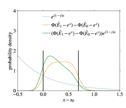
Figure 2: Weighting function in the computation of $\langle{\ln\hat{N}_{\mu}}\rangle\!^{\star}$. Shown on the x-axis is the logarithm $x=\ln E$ of the true air shower energy $E$. Thick vertical lines indicate the boundaries of an energy bin with $\Delta\log_{10}E=0.3$. A value of $\gamma=2.7$ is used for energy spectrum, the energy resolution is $10\,\%$.

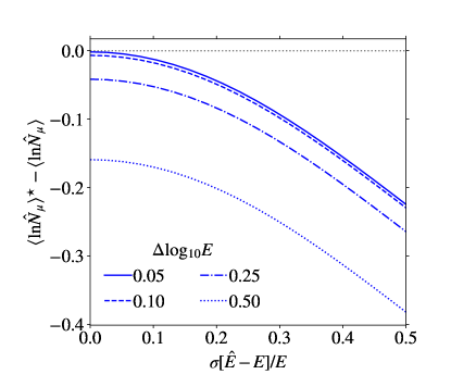
Figure 3: Binning bias for a $E^{-2.7}$ spectrum and $\beta=0.9$ as a function of the relative resolution of energy estimate $\hat{E}$.

To compute $\langle{\ln\hat{N}_{\mu}}\rangle^{\star}$, we to convolve the integrand in Eq. 12 with a energy resolution kernel. Usually, a normal distribution is appropriate

$$\mathcal{N}(\hat{E};E)=\frac{1}{\sqrt{2\pi}\sigma}e^{-\frac{1}{2}(\hat{E}-E)^{2}/\sigma^{2}},$$ (14)

which describes the probability to observe an energy estimate $\hat{E}$ with resolution $\sigma$ for a given true energy $E$. This leads to

$$\langle{\ln\hat{N}_{\mu}}\rangle\!^{\star}=\frac{\int_{\hat{E}_{0}}^{\hat{E}_{1}}\mathrm{d}\hat{E}\int_{-\infty}^{\infty}\mathrm{d}x\,\mathcal{N}(\hat{E};e^{x})(\ln N_{\mu}^{0}+\beta x)e^{(1-\gamma)x}}{\int_{\hat{E}_{0}}^{\hat{E}_{1}}\mathrm{d}\hat{E}\int_{-\infty}^{\infty}\mathrm{d}x\,\mathcal{N}(\hat{E};e^{x})e^{(1-\gamma)x}}$$

$$=\ln N_{\mu}^{0}+\frac{\int_{-\infty}^{\infty}\mathrm{d}x\,(\Phi(\hat{E}_{1};e^{x})-\Phi(\hat{E}_{0};e^{x}))\beta xe^{(1-\gamma)x}}{\int_{-\infty}^{\infty}\mathrm{d}x\,(\Phi(\hat{E}_{1};e^{x})-\Phi(\hat{E}_{0};e^{x}))e^{(1-\gamma)x}}.$$ (15)

The integration over $\hat{E}$ was carried out in the second step, turning the probability density function $\mathcal{N}(\hat{E};e^{x})$ into its cumulative density function $\Phi(\hat{E};e^{x})$. The weighting function for the integrand obtained in this way is illustrated in Fig. 2. Showers with true energies near the lower edge of the bin get a higher weight and that also showers outside the bin interval contribute.

The effective energy interval to consider is now wider and not well bounded. Eq. 15 can be approximated by a Taylor series for $\Delta x\ll 1$ and $\sigma/E\ll 1$, but at this point it is easier to just compute the bias numerically by solving the equation. Fig. 3 shows numerical solutions for several bin widths and energy resolutions.

The binning bias is comparable to the other biases previously considered. For a common bin width of 0.1 in $\log_{10}\hat{E}$, an energy resolution of 15 %, a spectral index $\gamma=2.7$, and $\beta=0.9$, the bias for $\langle{\ln\hat{N}_{\mu}}\rangle$ is $-0.03$. This translates into a bias of $-0.3$ for $\langle{\ln A}\rangle$, about 7 % of the proton-iron distance. This bias is making the composition appear lighter.

VI Conclusions

The impact of stochastic fluctuations in the number of muons and the shower energy as well as in their experimental estimates on the computation of $\langle{\ln A}\rangle$ was discussed. Only $\langle{\ln N_{\mu}}\rangle$ has a straight-forward relationship to the mean logarithmic mass $\langle{\ln A}\rangle$ of cosmic rays. The biases calculated here are typically smaller than 10 % of the proton-iron distance, but can be larger for detectors with poor resolution. Several may need to be added.

To get the smallest systematic uncertainty, the muon number should be measured event-by-event and the mean logarithmic muon number $\langle{\ln N_{\mu}}\rangle$ computed, correcting for resolution and binning effects. A computation based on the mean muon number $\langle{N_{\mu}}\rangle$ is possible, but requires a correction that depends on the size of the natural fluctuations of $N_{\mu}$ for showers of the same energy, more precisely on $\operatorname{Var}[(N_{\mu}-\langle{N_{\mu}}\rangle)/\langle{N_{\mu}}\rangle]$. This variance has to be measured or estimated from air shower simulations. If simulation results are reported, the variance $\operatorname{Var}[(N_{\mu}-\langle{N_{\mu}}\rangle)/\langle{N_{\mu}}\rangle]$ should generally be included.

VII Acknowledgments

I am grateful for valuable discussions about this topic with Lorenzo Cazon and Felix Riehn. I also thank the reviewers from Astroparticle Physics who kindly commented on this draft and gave it more focus.

Appendix A Parametrization of relative variance of muon number

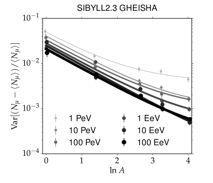
Figure 4: Variance of the relative deviation from the mean muon number as a function of logarithmic mass $\ln A$ of the primary cosmic ray, using the data from Table 1. Solid lines are fits described in the text.

The relative variance $\operatorname{Var}[(N_{\mu}-\langle N_{\mu}\rangle)/\langle N_{\mu}\rangle]$ of the muon number for primary cosmic rays with energy $E$ and mass $A$ plays an important role in section III. It is useful to have a parameterization for this quantity. Based on the numbers in Table 1, the evolution is shown as a function of $\ln A$ for several energies in Fig. 4. The simulations are well described by the model,

$$\operatorname{Var}[(N_{\mu}-\langle N_{\mu}\rangle)/\langle N_{\mu}\rangle]=p_{0}(E)+p_{1}(E)/A,$$ (16)

where $p_{0}$ and $p_{1}$ are energy-dependent parameters. The formula is motivated by the superposition model Matthews (2005), which states that an air shower with $A$ nucleons approximately behaves like a superposition of $A$ showers with an energy $E/A$. If the $A$ nucleons develop independently, the fluctuations in the individual sub-showers average out. This leads to a $1/A$ reduction in the variance. The other parameter $p_{0}$ summarizes correlated fluctuations which do not cancel, for example, fluctuations due to the depth of the first interaction.

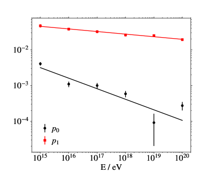
Figure 5: Energy dependence of the fluctuation parameters from Eq. 16. Lines represent the fits described in the text.

The energy-dependence of the parameters $p_{0}$ and $p_{1}$ is shown in Fig. 5 and well described by a power law,

$$p_{i}(E)=a_{i}\,(E/10^{15}\,\text{eV})^{b_{i}}$$ (17)

$$\begin{array}[]{l l}a_{0}&=0.00317\pm 0.00037\\ a_{1}&=0.0455\pm 0.0032\end{array}\quad\begin{array}[]{l l}b_{0}&=-0.295\pm 0.033\\ b_{1}&=-0.0727\pm 0.0095.\end{array}$$ (22)

These numerical values are valid for a set of pure primary cosmic rays with mass $A$ of vertical incidence, simulated with SIBYLL-2.3 in a standard atmosphere. To compute the variance for mixtures of primaries, the mean $\langle N_{\mu}\rangle$ also needs to be parametrized as a function of $A$, which can be done with a power-law as well.

Appendix B Taylor series

The following Taylor series are used in the paper:

$$\frac{1}{e^{(1-\gamma)x_{0}}x_{0}^{n}\Delta x}\int_{x_{0}}^{x_{0}+\Delta x}e^{(1-\gamma)x}x^{n}\mathrm{d}x\approx$$

$$1+\frac{\Delta x}{2}\left((1-\gamma)+\frac{n}{x_{0}}\right)$$

$$+\frac{\Delta x^{2}}{6}\left((1-\gamma)^{2}+\frac{2n(1-\gamma)}{x_{0}^{n-1}}+\frac{n(n-1)}{x_{0}^{n-2}}\right)$$

$$+\mathcal{O}(\Delta x^{3}),$$ (23)

$$\frac{a_{0}+a_{1}\Delta x+a_{2}\Delta x^{2}}{b_{0}+b_{1}\Delta x+b_{2}\Delta x^{2}}\approx$$

$$\frac{a_{0}}{b_{0}}+x\frac{a_{1}b_{0}-a_{0}b_{1}}{b_{0}^{2}}$$

$$+x^{2}\frac{a_{2}b_{0}^{2}-a_{1}b_{0}b_{1}+a_{0}(b_{1}^{2}-b_{0}b_{2})}{b_{0}^{3}}+\mathcal{O}(x^{3}).$$ (24)

Combining these two series, one gets

$$\frac{1}{x_{0}^{n}}\frac{\int_{x_{0}}^{x_{0}+\Delta x}e^{(1-\gamma)x}x^{n}\mathrm{d}x}{\int_{x_{0}}^{x_{0}+\Delta x}e^{(1-\gamma)x}\mathrm{d}x}\approx$$

$$1+\frac{\Delta x}{2}\frac{n}{x_{0}}+\frac{\Delta x^{2}}{6}\left(\frac{n(1-\gamma)}{2x_{0}}+\frac{n(n-1)}{x_{0}^{2}}\right)$$

$$+\mathcal{O}(\Delta x^{3}).$$ (25)

References

- Kampert and Unger (2012) K.-H. Kampert and M. Unger, Astropart. Phys. 35, 660 (2012), arXiv:1201.0018 [astro-ph.HE] .
- Aab et al. (2014) A. Aab et al. (Pierre Auger), JCAP 1408, 019 (2014), arXiv:1407.3214 [astro-ph.HE] .
- Abbasi et al. (2013) R. Abbasi et al. (IceCube), Nucl. Instrum. Meth. A700, 188 (2013), arXiv:1207.6326 [astro-ph.IM] .
- Apel et al. (2015) W. D. Apel et al., Astropart. Phys. 65, 55 (2015).
- Abu-Zayyad et al. (2000) T. Abu-Zayyad et al. (MIA, HiRes), Phys. Rev. Lett. 84, 4276 (2000), arXiv:astro-ph/9911144 [astro-ph] .
- Ave et al. (2000a) M. Ave, R. A. Vazquez, and E. Zas, Astropart. Phys. 14, 91 (2000a), arXiv:astro-ph/0011490 [astro-ph] .
- Ave et al. (2000b) M. Ave, R. A. Vazquez, E. Zas, J. A. Hinton, and A. A. Watson, Astropart. Phys. 14, 109 (2000b), arXiv:astro-ph/0003011 [astro-ph] .
- Dembinski et al. (2010) H. P. Dembinski, P. Billoir, O. Deligny, and T. Hebbeker, Astropart. Phys. 34, 128 (2010), arXiv:0904.2372 [astro-ph.IM] .
- Aab et al. (2015) A. Aab et al. (Pierre Auger), Phys. Rev. D91, 032003 (2015), [Erratum: Phys. Rev.D91,no.5,059901(2015)], arXiv:1408.1421 [astro-ph.HE] .
- Dembinski et al. (2016) H. P. Dembinski, B. Kégl, I. C. Mariş, M. Roth, and D. Veberič, Astropart. Phys. 73, 44 (2016), arXiv:1503.09027 [astro-ph.IM] .
- Abreu et al. (2013) P. Abreu et al. (Pierre Auger), JCAP 1302, 026 (2013), arXiv:1301.6637 [astro-ph.HE] .
- Matthews (2005) J. Matthews, Astropart. Phys. 22, 387 (2005).
- Heck et al. (1998) D. Heck et al., Report FZKA 6019, Tech. Rep. (FZK Karlsruhe, Germany, 1998).
- Riehn et al. (2015) F. Riehn, R. Engel, A. Fedynitch, T. K. Gaisser, and T. Stanev, “A new version of the event generator SIBYLL,” (2015), arXiv:1510.00568 [hep-ph] .
- Fesefeldt (1985) H. Fesefeldt, Report PITHA-85/02, RWTH Aachen (1985).
- Dembinski and Gonzalez (2016) H. P. Dembinski and J. Gonzalez, Proceedings, 34th International Cosmic Ray Conference (ICRC 2015): The Hague, The Netherlands, July 30-August 6, 2015, PoS ICRC2015, 267 (2016).
- Dembinski (2009) H. P. Dembinski, Measurement of the flux of ultra high energy cosmic rays using data from very inclined air showers at the Pierre Auger Observatory, Ph.D. thesis, RWTH Aachen University (2009).
- Lafferty and Wyatt (1995) G. D. Lafferty and T. R. Wyatt, Nucl. Instrum. Meth. A355, 541 (1995).
- Dembinski and Roth (2013) H. P. Dembinski and M. Roth, Nucl. Instrum. Meth. A729, 410 (2013).