A new method of measuring center-of-mass velocities of radially pulsating stars from high-resolution spectroscopy.

Abstract

We present a radial velocity analysis of 20 solar neighborhood RR Lyrae and 3 Population II Cepheids variables. We obtained high-resolution, moderate-to-high signal-to-noise ratio spectra for most stars and obtained spectra were covering different pulsation phases for each star. To estimate the gamma (center-of-mass) velocities of the program stars, we use two independent methods. The first, ‘classic’ method is based on RR Lyrae radial velocity curve templates. The second method is based on the analysis of absorption line profile asymmetry to determine both the pulsational and the gamma velocities. This second method is based on the Least Squares Deconvolution (LSD) technique applied to analyze the line asymmetry that occurs in the spectra. We obtain measurements of the pulsation component of the radial velocity with an accuracy of $\pm$ 3.5 km s^-1. The gamma velocity was determined with an accuracy $\pm$ 10 km s^-1, even for those stars having a small number of spectra. The main advantage of this method is the possibility to get the estimation of gamma velocity even from one spectroscopic observation with uncertain pulsation phase. A detailed investigation of the LSD profile asymmetry shows that the projection factor $p$ varies as a function of the pulsation phase – this is a key parameter which converts observed spectral line radial velocity variations into photospheric pulsation velocities. As a byproduct of our study, we present 41 densely-spaced synthetic grids of LSD profile bisectors that are based on atmospheric models of RR Lyr covering all pulsation phases.

1 Introduction

Table 1: Basic information for the program stars.

Star	R.A.(J2000)	Decl.(J2000)	Type	$V$	$\Delta V$	Epoch	Period
	(h m s)	($\degr$ $\arcmin$ $\arcsec$)		(mag)	(mag)	(JD 2400000$+$)	(day)
DR And	01 05 10.71	$+$34 13 06.3	RRab *	11.65 – 12.94	1.29	51453.158583	0.5631300
X Ari	03 08 30.88	$+$10 26 45.2	RRab	11.28 – 12.60	1.32	54107.2779	0.6511681
TW Boo	14 45 05.94	$+$41 01 44.1	RRab	10.63 – 11.68	1.05	53918.4570	0.53226977
TW Cap	20 14 28.42	$-$13 50 07.9	CWa	9.95 – 11.28	1.33	51450.139016	28.610100
RX Cet	00 33 38.28	$-$15 29 14.9	RRab *	11.01 – 11.75	0.74	52172.1923	0.5736856
U Com	12 40 03.20	$+$27 29 56.1	RRc	11.50 – 11.97	0.47	51608.348633	0.2927382
RV CrB	16 19 25.85	$+$29 42 47.6	RRc	11.14 – 11.70	0.56	51278.225393	0.3315650
UZ CVn	12 30 27.70	$+$40 30 31.9	RRab	11.30 – 12.00	0.70	51549.365683	0.6977829
SW CVn	12 40 55.03	$+$37 05 06.6	RRab	12.03 – 13.44	1.41	51307.226553	0.4416567
AE Dra	18 27 06.63	$+$55 29 32.8	RRab	12.40 – 13.38	0.98	51336.369463	0.6026728
BK Eri	02 49 55.88	$-$01 25 12.9	RRab	12.00 – 13.05	1.05	51462.198773	0.5481494
UY Eri	03 13 39.13	$-$10 26 32.4	CWb	10.93 – 11.66	0.73	51497.232193	2.2132350
SZ Gem	07 53 43.45	$+$19 16 23.9	RRab	10.98 – 12.25	1.27	51600.336523	0.5011365
VX Her	16 30 40.80	$+$18 22 00.6	RRab *	9.89 – 11.21	1.32	53919.451	0.45536088
DH Hya	09 00 14.83	$-$09 46 44.1	RRab	11.36 – 12.65	1.29	51526.426583	0.4889982
V Ind	21 11 29.91	$-$45 04 28.4	RRab	9.12 – 10.48	1.36	47812.668	0.479601
SS Leo	11 33 54.50	$-$00 02 00.0	RRab	10.38 – 11.56	1.18	53050.565	0.626335
V716 Oph	16 30 49.47	$-$05 30 19.5	CWb	8.97 – 9.95	0.98	51306.272953	1.1159157
VW Scl	01 18 14.97	$-$39 12 44.9	RRab	10.40 – 11.40	1.00	27809.381	0.5109147
BK Tuc	23 29 33.33	$-$72 32 40.0	RRab	12.40 – 13.30	0.90	36735.605	0.5502000
TU UMa	11 29 48.49	$+$30 04 02.4	RRab	9.26 – 10.24	0.98	51629.148846	0.5576587
RV UMa	13 33 18.09	$+$53 59 14.6	RRab	9.81 – 11.30	1.49	51335.380433	0.4680600
UV Vir	12 21 16.74	$+$00 22 03.0	RRab *	11.35 – 12.35	1.00	51579.459853	0.5870824

Notes. The coordinates (columns 2 and 3), variability class and stars with exhibiting the Blazhko effect (according to Skarka, 2013) are marked by an asterisk (column 4), magnitude ranges (column 5), amplitude of the magnitude variation (column 6), and pulsation periods (column 8) have been taken from the General Catalog of Variable Stars (GCVS, Samus et al., 2007). The epochs of maximum light (column 7) were extracted from the ROTSE light curves (see Paper I for more details).

RR Lyraes are important tracers of galactic dynamics and evolution. Their high luminosity makes them good tracers for investigations of the Galactic halo (e.g. Kollmeier et al., 2009) and of stellar systems outside the Milky Way (e.g. Stetson et al., 2014). Together with the proper motion, the center-of-mass velocity (or gamma velocity, $V_{\gamma}$) of this type of stars is thus a fundamental parameter that should be derived with the highest possible accuracy. With the Gaia satellite already measuring precise proper motions for thousands of variable stars in the Milky Way and beyond, the missing ingredient in a full determination of fundamental kinematic parameters for RR Lyrae stars is the estimate of gamma velocity. Indeed, the uncertainties associated to the determination of gamma velocities of RR Lyrae stars constitute a long-standing problem, which also affects the accuracy of RR Lyraes as distance indicators (e.g. Benedict et al., 2011). Several studies have been devoted to this problem (Hawley & Barnes, 1985; Jeffery et al., 2007; For et al., 2011; Sessar, 2012; Nemec et al., 2013). Traditionally, the approach to derive the gamma velocity relies on a template radial velocity curve, that is shifted and scaled to match the observed radial velocity at a few different phases (Liu, 1991). This method becomes more accurate when observations covering several phases are available. In this work, we apply a method which allows to estimate the gamma velocity of RR Lyrae stars from just a few observations obtained at random phases. The method is based on (i) investigations of the absorbtion line profile asymmetry that occurs during the radial pulsations and (ii) determination of the absolute value of the pulsation component using line profile bisectors, taking carefully into account limb-darkening effects. We test our method on a sample of solar neighborhood RR Lyraes that was investigated in a previous paper (Pancino et al., 2015, hereinafter Paper I) and on densely-spaced observations of RR Lyr (Fossati et al., 2014).

The paper is organized as follows: in Section 2 we briefly review the observations and data reduction for our sample stars. In Section 3, we discuss the determination of the radial velocity and gamma velocity when applying the ‘classic’ method based on radial velocity curve templates. Section 4 presents our method of bisectors for the determination of the gamma and pulsation velocities of RR Lyraes, and compares the results with those from the classical approach. Moreover, we tested our method on the high resolution observations of RR Lyr. Section 5 presents the results of the analysis; Section 6 closes the paper with the summary and conclusions. Appendix A presents an extensive library of synthetic bisectors that can be used to apply our proposed method to spectra of variable stars.

2 Observations and data reduction

The analysed sample consists of 20 RR Lyr stars and 3 Population II Cepheids. The stars were observed as part of different programs with the SARG (Gratton et al., 2001) echelle spectrograph at the Telescopio Nazionale Galileo (TNG, La Palma, Spain) and with the UVES (Dekker et al., 2000) spectrograph at ESO’s Very Large Telescope (VLT, Paranal, Chile). Furthermore, additional archival spectra were retrieved from the ESO archive. The resolving power of the spectra obtained with SARG is R = $\lambda/\delta\lambda\approx$ 30 000 with an average signal-to-noise ratio S/N $\approx$ 50-100 and spectral coverage from 4000 to 8500 Å. The UVES spectra have a higher resolving power, R $\approx$ 47 000, and S/N $\approx$ 70-150 and cover the wavelength range from 4500 to 7500 Å. The observations were performed at random pulsation phases generally three times for each star; however, for some stars we have more then 3 observations, or just one observation. Table 1 presents some general information about the program stars.

A full description of the observations and reduction process, including the determination of the fundamental parameters of the sample stars, is presented in Paper I. Briefly, SARG spectra were reduced with standard IRAF tasks in the echelle package, including bias and flat-field correction, spectral tracing, extraction, wavelength calibration, and continuum normalization. The typical r.m.s. deviation of wavelength calibration lines centroids from the two-dimensional fitted calibration polynomials was close to 0.03 Å. Sky absorption lines (telluric bands of O₂ and H₂O) were removed using the IRAF task telluric with the help of our own library of observed spectra. UVES spectra were reduced with the UVES pipeline (Ballester et al., 2000) as part of the service observations, and include similar steps as the ones described for SARG.

The dataset from Paper I was complemented by the densely spaced observations of RR Lyrae along the pulsation cycle described by Fossati et al. (2014).

3 Gamma velocity of pulsating stars

From an observational point of view, the gamma velocity, $V_{\gamma}$, can be described using the following equation:

$$V_{\gamma}=v_{obs}+v_{\odot}-v_{puls}\qquad(1)$$

where $v_{obs}$ is the observed velocity of the star along the line of sight, $v_{\odot}$ is the heliocentric correction, and $v_{puls}$ is the pulsation velocity of the radially pulsating star. We will see in the following sections that the determination of $v_{puls}$ requires a treatment of limb-darkening effects, generally included in the form of a projection factor. The sum $v_{obs}+v_{\odot}$ is the heliocentric radial velocity of the star, $v_{rad}$, at any given phase in the pulsation cycle. In other words, the determination of the gamma velocity of pulsating stars such as RR Lyraes and Cepheids requires — in principle — the determination of two quantities: (i) the observed radial velocity (reported to the heliocentric reference) and (ii) the pulsation component at the moment of the observation or, better, at the specific pulsation phase of the observations (corrected for limb-darkening effects).

In the next subsections we apply the most widely used method for deriving the gamma velocity to the sample described in Section 2. The resulting measurements (reported in Table 2) are then used as reference values to test the method based on bisectors (Section 4).

3.1 Measurement of $v_{obs}$ using cross-correlation

We first measured the radial velocity of our sample spectra using the classical cross-correlation method, implemented in the IRAF fxcor task and based on the standard Tonry & Davis (1979) algorithm. We cross-correlated the observed spectra with synthetic spectra generated with the latest modified version (15 March 2013) of the STARSP-SynthV package, an LTE spectral synthesis code developed by Tsymbal (1996), which uses ATLAS9 (Kurucz, 1993) grids of stellar atmosphere models. We adopted the following typical atmospheric parameters of RR Lyr stars for the synthetic spectrum generation: $T_{\mathrm{eff}}$ = 6250 K, $\log g=2.5$ dex, $v_{mic}=2.0$ km s^-1 – as the typical values at quiescent phases along the RR lyrae stars pulsation cycle from Paper I. Then, we convolved the synthetic spectrum with a Gaussian to reproduce the spectral resolution of the observed spectra (Section 2). We performed a cross-correlation analysis for all spectra in the wavelength range 5100 - 5400 $\AA$, where several prominent, not blended, Ti and Fe lines are present. We remark that the low metallicity of RR Lyrae stars leads to a limited line blending.

The resulting radial velocity measurements derived by the cross-correlation method ($v_{obs}^{Xcor}$) and their errors, $\delta v_{obs}^{Xcor}$ as estimated by the position and full width at half maximum of the cross-correlation peak, are reported in Table 2, along with their heliocentric corrections, $v_{\odot}$.

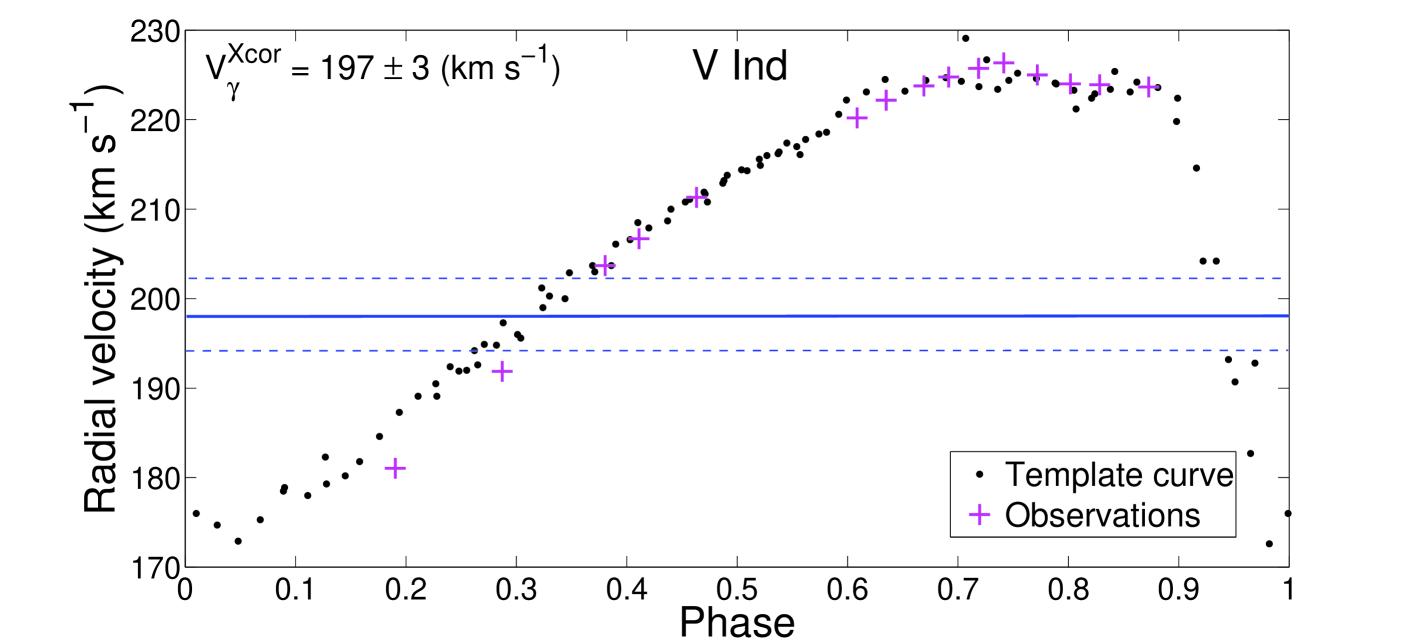
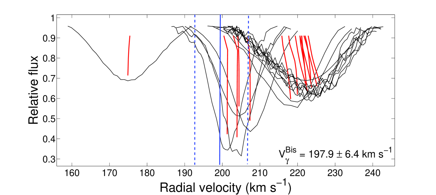
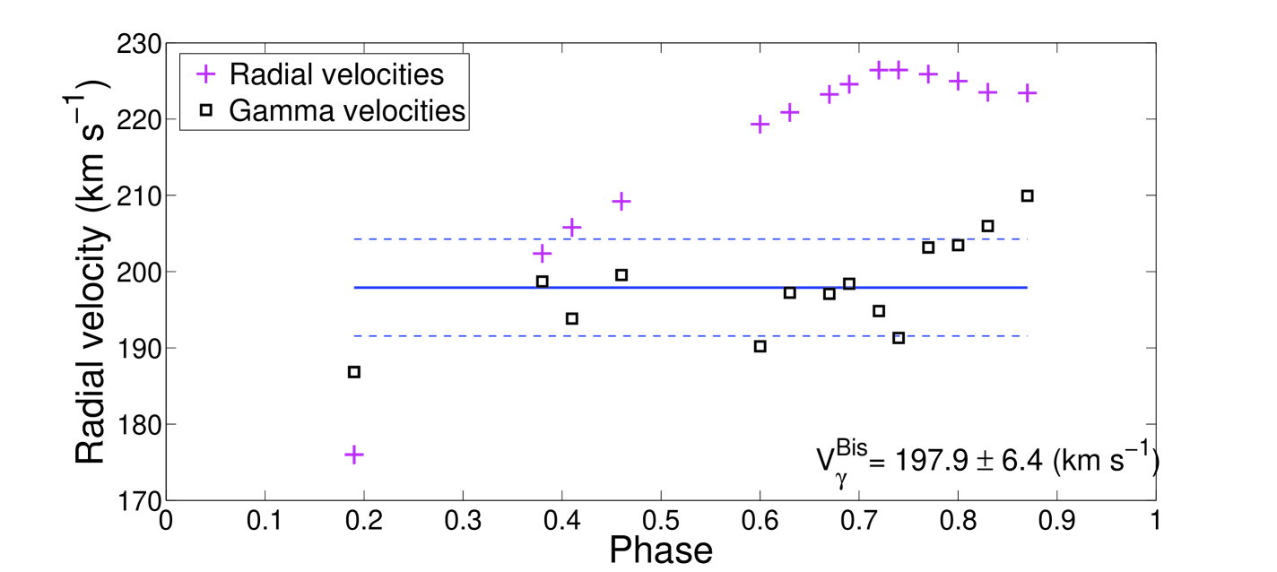
Figure 1: Examples of gamma velocity estimates for V Ind, obtained with a reference radial velocity curve (Clementini et al., 1990, top panel, see also Section 3) and with the bisectors method (middle and bottom panel, see Section 4), which has several spectra obtained at different phases. In the middle panel we present the individual LSD profiles together with their bisectors, the bottom panel shows the observed radial velocities (pink crosses) and derived individual values of gamma velocity (black boxes). The resulting gamma velocity is marked by blue solid line in all panels, the dashed lines showing the errors associated to each determination.

3.2 Measurement of $V_{\gamma}$ using velocity curve templates

We used the classical radial velocity curve template approach to obtain the final $V_{\gamma}^{Xcor}$, which is also reported in Table 2. The method relies on the use of an appropriate template radial velocity curve, that is fitted to the observed radial velocity points, to obtain the systemic or gamma velocity of the variable star. In our sample we have RRab Lyrae (fundamental mode pulsators), and RRc Lyrae (first overtone pulsators). The former present asymmetric lightcurves with large radial velocity and magnitude ($\delta V\approx$ 0.5–2 mag) variations. The latter, instead, have relatively symmetric lightcurves with smaller magnitude and radial velocity variations. The physics of RRc type variability is still poorly understood (see conclusions in Moskalik et al., 2015), mainly because of the presence of several radial and non radial pulsation modes. Thus, in our analysis for RRc type stars we used as a reference the average radial velocity curves of well known RRc Lyraes with similar radial velocity amplitudes. For a few of our RRab stars, we could rely on existing radial velocity curves from the literature: V Ind (Clementini et al., 1990); X Ari (Jones et al., 1987); TU Uma (Liu & Janes, 1989); U Com (Beers et al., 2000). For these stars the Baade-Wesselink (B-W) method was applied in the literature, thus the reliable radial velocity curves are exist for this sample. We noted that the typical amplitudes of these curves were all around 60 km s^-1. For the RRc type variables in our sample, we used the velocity curves of DH Peg (Jones et al., 1988) and YZ Cap (Cacciari et al., 1987), both with amplitudes of $\simeq$25 km s^-1. For the three Cepheids, TW Cap, V716 Oph, and UY Eri we used the radial velocity curve of W Vir (Sanford, 1952).

Table 2: Radial and gamma velocities of program stars, derived with the classical cross-correlation and radial velocity curves approach.

Star	Inst.	Exp	Phase	$v_{obs}^{Xcor}$	$\delta v_{obs}^{Xcor}$	$v_{\odot}$	$v_{rad}^{Xcor}$	$V_{\gamma}^{Xcor}$	$\delta V_{\gamma}^{Xcor}$
				(km s-1)	(km s-1)	(km s-1)	(km s-1)	(km s-1)	(km s-1)
DR And	SARG	1	0.63	–119.67	0.25	17.59	–102.08	–109.7	3.0
	SARG	2	0.69	–116.33	0.26	17.53	–98.80	–125.4	3.1
	SARG	3	0.31	–118.91	0.12	6.91	–112.00	–123.1	3.4
X Ari	APO	1	0.19	–23.25	0.26	–27.19	–50.44	–36.1	3.6
TW Boo	SARG	1	0.61	–83.20	0.12	3.11	–80.09	–101.1	1.5
	SARG	2	0.65	–80.67	0.13	3.11	–77.56	–100.4	1.6
	SARG	3	0.69	–79.87	0.13	3.07	–76.81	–100.3	1.4
TW Cap	UVES	1	0.54	–46.60	0.13	–15.68	–62.28	–72.3	5.0
RX Cet	SARG	1	0.51	–75.79	0.22	–4.34	–80.13	–93.7	3.1
U Com	SARG	1	0.06	–13.46	0.17	–5.55	–19.01	–7.8	3.2
	SARG	2	0.14	–8.42	0.14	–5.58	–14.00	–5.6	3.2
	SARG	3	0.21	–4.34	0.11	–5.61	–9.95	–7.1	3.2
RV CrB	SARG	1	0.35	–147.40	0.19	13.70	–133.70	–138.3	3.6
	SARG	2	0.42	–146.20	0.28	13.66	–132.54	–139.8	3.7
	SARG	3	0.48	–147.40	0.70	13.62	–133.78	–142.4	3.7
SW CVn	SARG	2	0.21	19.19	0.30	–7.80	11.39	24.0	3.9
	SARG	3	0.28	17.44	0.49	–7.86	9.58	16.5	3.1
UZ CVn	SARG	1	0.04	–39.35	0.18	–8.70	–47.44	–19.6	4.1
	SARG	2	0.08	–33.10	0.11	–8.77	–41.52	–17.1	3.5
	SARG	3	0.13	–29.41	0.12	–8.84	–37.90	–18.2	4.0
AE Dra	SARG	1	0.05	–309.69	0.18	6.03	–303.66	–275.7	1.7
	SARG	2	0.10	–304.91	0.17	5.99	–298.92	–275.3	1.7
BK Eri	UVES	1	0.04	95.33	0.69	–27.12	68.20	98.6	1.7
	UVES	2	0.20	109.29	0.16	–27.03	82.26	97.2	1.5
	UVES	3	0.14	102.80	0.21	–27.04	75.76	95.8	1.7
	UVES	4	0.51	137.82	0.08	–26.83	110.99	96.3	1.8
UY Eri	SARG	1	0.38	129.09	0.24	21.16	150.25	151.9	5.0
SZ Gem	SARG	1	0.50	309.44	0.23	26.93	336.37	321.6	3.0
VX Her	SARG	1	0.86	–370.87	0.13	18.47	–351.96	–340.1	5.3
	SARG	2	0.05	–391.85	0.98	18.43	–373.33	–402.4	4.8
DH Hya	UVES	1	0.79	389.03	0.18	–24.17	364.86	336.3	4.5
	SARG	2	0.71	381.25	0.15	–20.06	361.18	334.1	5.2
	SARG	3	0.79	385.19	0.26	–20.17	365.02	334.3	4.3
V Ind	UVES	1	0.19	175.00	0.22	6.03	181.03	194.9	4.6
	UVES	2	0.29	204.00	0.09	–12.13	191.87	196.1	3.3
	FEROS	1	0.46	208.00	0.08	3.31	211.31	197.1	3.1
	FEROS	2	0.60	217.00	0.11	3.20	220.20	198.3	3.0
	FEROS	3	0.63	219.00	0.11	3.18	222.18	198.0	3.1
	HARPS	1	0.67	221.00	0.24	2.77	223.77	196.3	3.0
	HARPS	2	0.69	222.00	0.24	2.77	224.77	197.6	3.0
	HARPS	3	0.72	223.00	0.26	2.74	225.74	198.2	3.0
	HARPS	4	0.38	201.00	0.17	2.69	203.69	198.9	3.2
	HARPS	5	0.41	204.00	0.21	2.69	206.69	199.3	3.8
	HARPS	6	0.74	224.00	0.28	2.34	226.34	198.0	4.9
	HARPS	7	0.77	223.00	0.33	2.00	225.00	196.2	6.1
	HARPS	8	0.80	222.00	0.33	2.00	224.00	194.4	9.8
	HARPS	9	0.83	222.00	0.27	1.90	223.90	193.2	8.4
	HARPS	10	0.87	221.78	0.21	1.87	223.65	194.5	7.5
SS Leo	UVES	1	0.06	156.83	0.23	–20.77	136.06	165.4	4.1
	UVES	2	0.07	155.53	0.25	–20.79	134.74	162.2	3.9
V716 Oph	UVES	1	0.08	–307.06	0.11	–28.25	–335.31	–310.8	5.0
VW Scl	UVES	1	0.71	86.85	0.12	–25.91	67.02	40.3	3.2
	UVES	2	0.23	57.41	0.09	–25.83	31.58	41.0	3.0
	UVES	3	0.32	65.86	0.06	–25.59	40.27	41.2	3.1
	UVES	4	0.15	47.69	0.15	–25.41	22.28	42.2	3.0
	UVES	5	0.05	37.76	0.37	–25.63	12.13	37.7	3.2
BK Tuc	UVES	1	0.17	162.49	0.12	–2.52	159.97	167.4	3.1
	UVES	2	0.26	162.25	0.15	–2.57	159.68	174.4	3.1
	UVES	3	0.15	160.86	0.11	–2.86	158.00	167.4	3.1
TU UMa	SARG	1	0.45	122.65	0.10	–13.15	109.50	99.4	3.0
RV Uma	SARG	1	0.62	–171.26	0.16	–5.61	–176.87	–200.1	3.9
	SARG	2	0.66	–167.39	0.14	–5.64	–173.03	–198.8	3.7
	SARG	3	0.71	–164.40	0.15	–5.67	–170.07	–196.2	5.9
UV Vir	UVES	1	0.87	74.20	0.18	–16.58	57.62	99.4	3.0

For the remaining stars, we reconstructed synthetic radial velocity curves following Liu (1991), who provided both a template radial velocity curve for RRab stars and a correlation between the amplitudes of the light curves and radial velocity curves, based on a large sample of RR Lyrae observations. We used the magnitude ranges reported in Table 1 to obtain radial velocity amplitudes with equation (1) by Liu (1991). We then divided the obtained amplitude by an average projection factor of 1.3 (see also Section 4.5), and scaled the template curve appropriately. We then adjusted the template curve to our measured radial velocities – an example of this procedure is shown in Figure 1 (top panel) for V Ind, which has several spectra at different phases. The final gamma velocity is obtained as an average of the (scaled and shifted) radial velocity curve that fits the observational points.

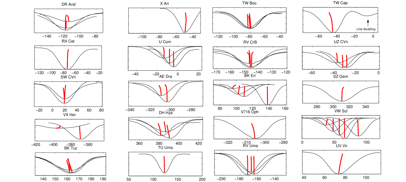
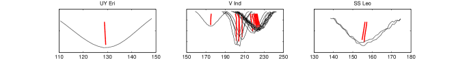
Figure 2: LSD profiles (black lines) and bisectors (red lines) for all sample spectra. The x-axis gives the velocity in km s^-1.

The typical uncertainties connected to the use of this method depend on several factors. As discussed by Liu (1991, see also ), the error in the normalization of the radial velocity curve is about 3 km s^-1, to which one has to add the individual radial velocity uncertainties (Table 2). Additionally, whenever an observed radial velocity curve was available in the literature, we repeated the analysis with the observed curve and compared the results. In each case, the results obtained with the two methods were comparable — i.e., no systematic differences were found — so we used a weighted average of the results obtained with the template and observed curve.

4 Bisectors method

The classical method described above provides good results when a good phase sampling is available, or, in case of few observations, when the phase of the observations is well known. In this section we discuss an alternative method for the determination of the gamma velocity, based on the asymmetry of line profiles in pulsating stars, that vary along the pulsation cycle and thus can also be used to infer the pulsational velocity. This method, hereafter referred to as bisectors method for brevity, allows for an estimate of the gamma velocity of pulsating stars with a sparse phase sampling, and it works even with just one observation, albeit with a slightly larger uncertainty. In the literature, this method was mentioned by several authors (e.g. Hatzes A., 1996; Gray, 2010). Other authors (e.g. Sabbey et al., 1995; Nardetto et al., 2008, 2013) use the Gaussian asymmetry coefficient to estimate line asymmetries and perform the same task, however, the bisectors method allows for a more detailed study of the line profile, i.e., to study line asymmetries and v_puls variations at different depths inside the stellar atmosphere. On the other hand, the bisectors method is in general more sensitive to the spectra quality, i.e., S/N ratio, spectral resolution, and line crowding and blending.

To derive average line profiles, we use the LSD method (Least-Square Deconvolution, Donati et al., 1997), that infers a very high S/N ratio line profile for each spectrum from the profiles of many observed absorption lines, under the assumption that the vast majority of lines have the same shape, and that different line components add up linearly (Kochukhov et al., 2010). Depending on the number of used lines, the reconstructed LSD profile can have an extremely high S/N ratio, rarely attainable with RR Lyrae observations on single lines. The problem with RR Lyrae is that it is difficult to make long exposure observations without avoiding the line smearing effect, as a result its limit the S/N of obtained spectra. The original LSD method by Donati et al. (1997) was modified and extended to different applications by several authors (e.g., Kochukhov et al., 2010; Van Reeth et al., 2013; Tkachenko et al., 2013, among others). We used the Tkachenko et al. (2013) implementation (see next section), and our workflow can be outlined as follows:

1. we compute the LSD profile of each observed spectrum; this also allows for an independent estimate of $v_{obs}$ (Section 4.1);

2. we compute a theoretical library of LSD profiles (Appendix A), predicting the line profile asymmetries at each pulsation phase, and compute the bisectors of each of the profiles; the theoretical bisectors library is made available in the electronic version of this paper and can be used to derive $v_{obs}$ and $V_{\gamma}$ for RR Lyrae observations obtained at unknown or poorly determined phases;

3. we compute the bisector of the observed LSD line profile and compare that to the ones in our theoretical library, to determine which pulsation velocity corresponds to the observed asymmetry of the LSD bisector (Section 4.2); in our computation, we implement a full description of limb-darkening effects (Section 4.5).

Once the observed and pulsational components are known, the gamma velocity can be trivially obtained from equation (1).

Table 3: Radial, pulsational and gamma velocities of program stars, derived with the LSD profile and the bisector’s method.

Star	Inst.	Exp	Phase	$v_{obs}^{LSD}$	$\delta v_{obs}^{LSD}$	$v_{rad}^{LSD}$-$V_{\gamma}^{Bis}$	$v_{puls}^{Bis}$	$\delta v_{puls}^{Bis}$	$V_{\gamma}^{Bis}$	$\delta V_{\gamma}^{Bis}$
				($km~{}s^{-1}$)	($km~{}s^{-1}$)	($km~{}s^{-1}$)	($km~{}s^{-1}$)	($km~{}s^{-1}$)	($km~{}s^{-1}$)	($km~{}s^{-1}$)
DR And	SARG	1	0.63	–119.8	0.5	5.2	5	5.0	–107.4	5.9
	SARG	2	0.69	–115.0	0.9	16.8	20	0.6	–114.2	1.5
	SARG	3	0.31	–118.6	0.5	–2.6	–5	1.0	–109.0	3.3
X Ari	APO	1	0.19	–51.1	1.3	–34.3	–43	2.0	–43.9	2.6
TW Boo	SARG	1	0.61	–83.0	1.7	8.1	10	5.0	–88.0	5.4
	SARG	2	0.65	–80.3	1.2	11.4	13	1.5	–88.6	2.1
	SARG	3	0.69	–79.2	0.2	14.3	17	1.9	–90.4	2.2
TW Cap	UVES	1	0.54	–46.1	1.1	25.4	30	1.0	–87.2	1.8
RX Cet	SARG	1	0.51	–75.5	0.5	–11.8	–17	2.1	–68.0	2.4
U Com	SARG	1	0.87	–13.5	0.1	4.3	4	2.0	–23.3	3.7
	SARG	2	0.95	–8.1	0.2	7.8	1	1.0	–15.9	1.5
	SARG	3	0.02	–4.0	1.1	3.2	3	5.0	–12.8	6.1
RV CrB	SARG	1	0.35	–146.5	0.4	5.2	5	3.8	–137.9	4.9
	SARG	2	0.42	–145.3	0.8	–0.1	–2	6.3	–131.5	7.1
	SARG	3	0.48	–147.3	0.2	–3.1	–6	2.5	–130.5	2.7
SW CVn	SARG	2	0.21	17.8	2.0	–0.1	–2	3.3	10.1	5.4
	SARG	3	0.28	17.7	1.0	–7.7	–12	2.9	17.6	3.2
UZ CVn	SARG	1	0.04	–38.1	0.2	–0.1	–2	5.0	–46.0	5.9
	SARG	2	0.08	–32.9	0.2	14.2	17	0.5	–55.9	1.2
	SARG	3	0.13	–29.0	0.1	7.9	10	0.5	–45.7	1.2
AE Dra	SARG	1	0.05	–309.3	0.6	11.3	13	1.0	–314.5	1.6
	SARG	2	0.10	–304.6	0.4	9.7	11	5.0	–308.3	5.1
BK Eri	UVES	1	0.04	95.0	0.1	–14.3	–17	1.5	82.2	1.9
	UVES	2	0.20	109.2	0.1	–11.8	–16	0.5	93.9	1.2
	UVES	3	0.14	102.3	0.7	–13.3	–19	1.0	88.6	1.6
	UVES	4	0.51	138.1	0.2	2.7	1	3.0	108.6	4.3
UY Eri	SARG	1	0.38	129.3	1.1	4.4	4	4.5	146.1	5.7
SZ Gem	SARG	1	0.50	310.2	0.2	–8.9	–13	3.9	346.0	4.1
VX Her	SARG	1	0.86	–370.7	0.8	7.1	8	5.0	–359.3	5.2
	SARG	2	0.05	–397.3	0.9	–34.0	–43	2.0	–344.9	2.4
DH Hya	UVES	1	0.79	390.1	1.2	27.9	33	1.5	338.1	2.1
	SARG	2	0.71	381.8	0.5	24.2	29	5.0	337.5	5.1
	SARG	3	0.79	385.8	1.1	–2.7	–5	8.0	368.5	8.7
V Ind	UVES	1	0.19	174.9	0.1	–11.8	–17	0.6	192.7	1.3
	UVES	2	0.29	204.4	0.1	–1.9	–4	3.5	194.2	4.7
	FEROS	1	0.46	207.5	0.2	5.2	5	3.1	205.6	4.5
	FEROS	2	0.60	218.4	1.6	31.3	38	0.5	190.3	2.0
	FEROS	3	0.63	220.0	0.1	15.8	19	5.0	207.4	7.1
	HARPS	1	0.67	223.1	0.6	36.1	43	0.5	189.7	1.3
	HARPS	2	0.69	224.1	1.3	36.1	43	0.5	190.8	1.8
	HARPS	3	0.72	225.6	0.7	14.3	17	1.0	208.4	1.9
	HARPS	4	0.38	201.3	0.2	–10.7	–16	3.5	214.7	3.6
	HARPS	5	0.41	203.9	1.2	–7.2	–11	1.9	213.9	2.4
	HARPS	6	0.74	226.5	1.0	36.1	43	0.5	192.7	1.5
	HARPS	7	0.77	223.7	1.3	15.7	19	0.5	210.0	1.7
	HARPS	8	0.80	222.5	1.2	19.5	24	1.0	205.0	1.9
	HARPS	9	0.83	222.5	0.5	22.3	27	3.7	202.1	3.8
	HARPS	10	0.87	222.3	0.2	18.4	22	2.1	205.8	2.4
SS Leo	UVES	1	0.06	155.7	0.5	–23.2	–32	0.5	158.1	1.1
	UVES	2	0.07	154.6	1.1	–23.1	–31	2.6	156.8	3.0
V716 Oph	UVES	1	0.08	–305.8	1.2	36.0	43	0.5	–370.1	1.7
VW Scl	UVES	1	0.71	87.2	1.5	5.2	4	0.5	56.1	3.8
	UVES	2	0.23	57.4	0.7	–0.7	–1	2.5	32.3	4.0
	UVES	3	0.32	65.8	0.4	1.2	0	5.0	39.1	5.8
	UVES	4	0.15	47.6	0.3	–7.3	11	3.5	29.4	3.6
	UVES	5	0.05	36.9	0.5	–13.1	–17	1.2	24.4	1.7
BK Tuc	UVES	1	0.17	164.3	0.2	33.8	40	1.7	128.0	2.0
	UVES	2	0.26	162.7	0.8	19.1	23	4.3	141.1	4.5
	UVES	3	0.15	162.1	1.0	25.6	31	2.2	133.7	2.6
TU UMa	SARG	1	0.45	122.9	0.6	3.2	3	2.5	106.5	4.0
RV Uma	SARG	1	0.62	–171.6	0.1	2.7	1	1.5	–179.9	3.4
	SARG	2	0.66	–167.5	2.0	1.2	0	5.0	–174.3	6.5
	SARG	3	0.71	–164.2	0.4	1.2	0	5.0	–171.1	5.8
UV Vir	UVES	1	0.87	73.4	0.2	–23.4	–32	2.0	80.8	2.3

4.1 Measurement of $v_{obs}$ using LSD profiles

The LSD method for computing the line profile requires a list of spectral lines, specified by their central peak position and depth, or central intensity, which is generally referred to as a line mask. The whole spectrum is thus modeled as the convolution of an ideal line profile (assumed identical for all lines) with the actual pattern of lines from the mask. The LSD line profile is obtained by deconvolution from the line pattern, given an observed spectrum. Because the whole computation takes place in velocity space, the actual LSD profile carries the $v_{obs}$ information, in our particular case determined as the center-of-mass of the profile (Hareter et al., 2008; Kochukhov et al., 2010).

We built our line mask from the same line list that was used for our abundance analysis in Paper I, and there described in detail. Briefly, we selected all isolated lines that were well measured (errors below 20%) in at least three of the available spectra. For the line measurements we used DAOSPEC (Stetson & Pancino, 2008). After the abundance analysis, performed with GALA (Mucciarelli et al., 2013), all lines that gave systematically discrepant abundances, or that were systematically rejected because of their strengths or relative errors, were purged from the list. The final line list consisted of 352 isolated lines belonging to 9 different chemical species (see Paper I).

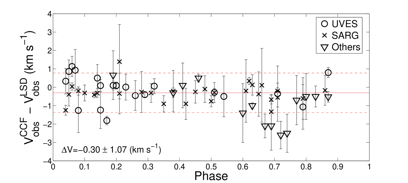
Figure 3: Differences between radial velocity estimates derived with the cross-correlation method, $v_{obs}^{Xcor}$, and with the LSD profile method, $v_{obs}^{LSD}$. The observations from the different spectrographs are labeled respectively.

We used the LSD code described by Tkachenko et al. (2013), which is a generalization of the original method by Donati et al. (1997). We applied the method in the wavelength range 5100–5400 $\AA$, that contains 155 of the above mentioned lines from Paper I.

Figure 2 displays the results of the computation. The resulting $v_{obs}^{LSD}$ are reported in Table 3, along with their errors, $\delta v_{obs}^{LSD}$. To evaluate the final errors, we evaluated different possible error sources and we summed them in quadrature. A first uncertainty is the difference between the minimum of the LSD profile and its center-of-mass, typically in the range 0.5–1 km s^-1. Since the line selection can have an impact on the line profiles, we repeated our measurements with three different line lists — using lines with a depth lower than 65%, 75%, and 85% of the continuum level — and used the dispersion in the resulting radial velocity as the uncertainty caused by the line selection procedure, obtaining values typically around 0.5 km s^-1. We note that V Ind has more observations along the pulsation cycle than other stars in the sample, which makes it the perfect test case for our method. The LSD profiles for V Ind are displayed in the lower panel of Figure 1, where the variation of the line shape with phase is clearly visible in both the line shape asymmetry and the bisectors slope.

Finally, we compared the $v_{obs}$ obtained with the classical cross-correlation method with those obtained with the LSD profile method (Figure 3), and found an extremely good agreement, with an average offset of 0.3 km s^-1 and a spread generally below 1 km s^-1, which is compatible with the individual error estimates of the two methods.

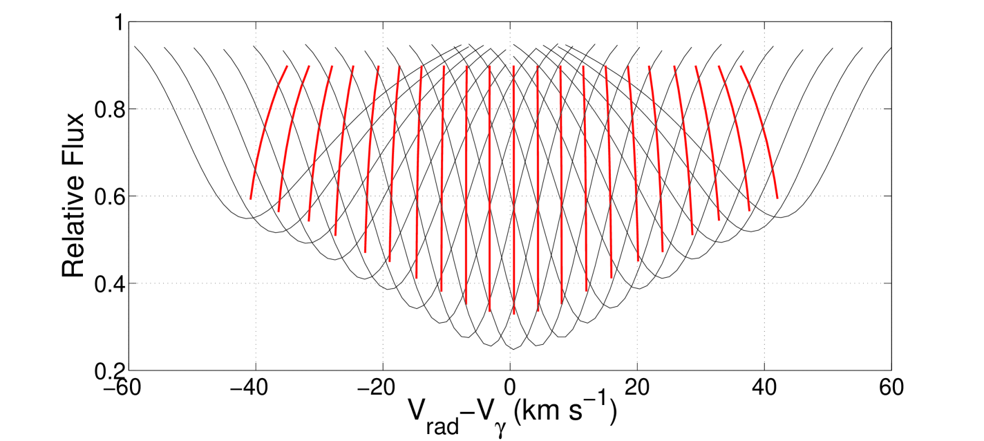
Figure 4: Example of LSD profiles and bisectors computed from model spectra of RR Lyrae (that corresponds to $\phi$=0.213, or spectrum number 087 in Fossati et al., 2014) with pulsation velocities from $-50$ to $+50$ km s^-1 with a step $5$ km s^-1.

The star TW Cap in our sample deserves particular attention. This star is a well known peculiar Type II Cepheid (Maas et al., 2007). The LSD profile shows a double minimum (see Figure 2), hinting at the line doubling phenomenon. Moreover, a double emission peak in $H_{\beta}$ is clearly visible in our spectrum. Wallerstein (1958) was the first to report about double lines in the spectra of TW Cap. These features could be explained by the existence of supersonic shock waves in the atmosphere at our observation phase ($\phi=0.54$). The same phenomenon is observed during shock phases in the spectra of RR Lyr (Chadid et al., 2008).

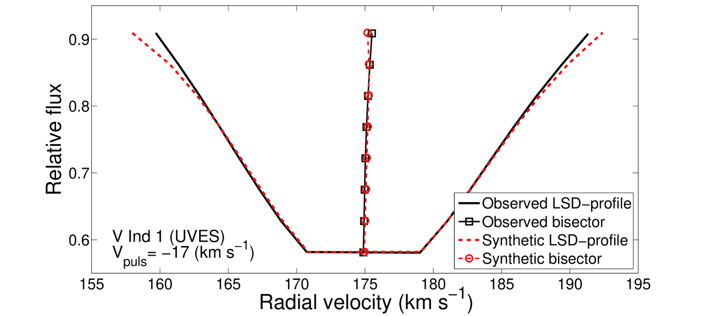
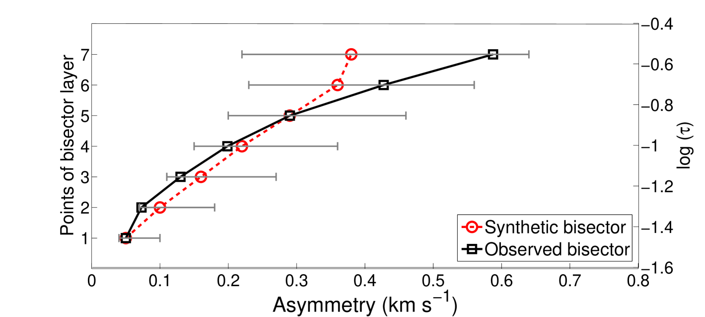
Figure 5: Comparison of the observed (black solid) and best fitting theoretical (red dashed) LSD profiles (top panel) and bisectors (bottom panel) for our first V Ind spectrum ($\phi$=0.19, see Table 3). The best fit corresponds to $v_{puls}$=–17$\pm$1 km s^-1. The grey error bars in the bottom panel correspond to the estimated errors on the method for determining $v_{puls}$, i.e., 1 km s^-1. The optical depth scale on the right ordinates axis was computed from synthetic spectra built with the atmospheric parameters derived in Paper I: $T_{\mathrm{eff}}$=7000 K, $\log~{}g=2.3$ dex, $v_{\mathrm{mic}}=1.6$ km s^-1, and [Fe/H]=$-$1.3 dex. The divergence between the observed and theoretical bisectors on layer 7 are caused by the lower S/N ratio of the LSD profile in this layer (see text for details). While the model bisector does not follow exactly the shape of the observed ones, the two agree reasonably well within the uncertainties.

4.2 Measurement of $v_{puls}$ using line bisectors

For a quantitative characterization of the LSD profile asymmetry, we used the bisector technique, which is a widely used diagnostic of line asymmetries (e.g. Gray, 2010). For each LSD profile, we computed the bisector of eight equally spaced depth layers, starting from a level of relative flux equal to 0.91 and reaching to the bottom of the line profile, at a flux level varying from 0.46 to 0.77, depending on the spectrum. The upper layer of the LSD profile, however, was found to be relatively uncertain, partly because we restricted ourselves to a small wavelength region and partly because of the paucity of lines in some of the analyzed spectra, caused by the low metallicity. Therefore, in the following, only the lowest seven layers will be employed (with relative flux below 0.85). The observed bisectors are shown in Figure 2 together with the computed LSD profiles.

To derive the pulsational velocity, $v_{puls}$, we compared the observed bisectors with a library of theoretical bisectors specifically computed for the program stars. The library is described in details in Appendix A and is publicly available in the electronic version of this paper and in CDS. One grid of theoretical LSD profiles and bisectors is shown on Figure 4, as an example. To find the best-matching theoretical bisector for each observed bisector, we minimized the quadratic difference between the two

$$\sqrt{\sum_{n=1}^{n=7}(Bis_{n}^{Obs}-Bis_{n}^{Templ})^{2}}$$

where 7 is the number of bisector points we take into account in the analysis (see above), and $Bis_{n}^{Obs}$ and $Bis_{n}^{Templ}$ are the values of the bisector evaluated at each layer of the observed and theoretical LSD profiles, respectively. In those cases where the exact phase of the observation is unknown, one can proceed in two steps. First, a blind comparison with the entire library is performed, providing an indication of the phase, and then a second iteration with the appropriate bisectors for that phase can be run.

Figure 5 illustrates, as an example, the best fit obtained with this technique for our first exposure of V Ind (see Table 3).

4.3 A test on RR Lyr

In order to test the method, we applied it to the prototype of the RR Lyrae class: RR Lyr itself. We used the 41 high-resolution (R=60 000) and high signal-to-noise (100–300) spectra of RR Lyr taken along the whole pulsation cycle analysed by Kolenberg et al. (2010); Fossati et al. (2014). In the following papers authors determined the phase dependent atmospheric parameters of RR Lyr based on which we compute the synthetic spectra and theoretical bisectors for each of 41 observations of RR Lyr. Thus, the number and IDs of each spectrum of RR Lyr from Fossati et al. (2014) are the same as the number of theoretical stellar atmosphere models which we used for constructing the grid of synthetic bisectors (see Appendix A). The good phase sampling allows us to test the method thoroughly along the whole pulsation cycle. In the table 4 the first three column present basic information about the set of RR Lyr spectra from Kolenberg et al. (2010); Fossati et al. (2014) which we used for computing synthetic spectra and constructing our grids of bisectors.

Table 4: Radial velocity measurements for the 41 spectra of RR Lyr from Kolenberg et al. (2010).

Number	Spectrum ID*	Phase	$T_{eff}$**	v${}_{obs}^{LSD}$	$\delta$v${}_{obs}^{LSD}$	vpuls	vpuls/(p-factor)	V${}_{\gamma}^{Bis}$	$\delta$V${}_{\gamma}^{Bis}$	p-factor
				(km s-1)	(km s-1)	(km s-1)	(km s-1)	(km s-1)	(km s-1)
1	87	0.173	6325 $\pm$ 50	–93.05	0.87	–11	–7.69	–85.36	2.67	1.43
2	88	0.207	6275 $\pm$ 50	–89.56	0.65	–11	–7.74	–81.83	6.86	1.42
3	89	0.229	6225 $\pm$ 50	–87.27	0.58	–11	–7.74	–79.53	7.76	1.42
4	91	0.260	6175 $\pm$ 100	–83.20	0.59	–11	–7.74	–75.46	6.85	1.42
5	120	0.846	6125 $\pm$ 100	–59.12	1.50	19	15.11	–74.23	1.50	1.26
6	121	0.868	6375 $\pm$ 100	–67.33	0.95	3	3.02	–70.35	0.88	0.99
7	122	0.890	6725 $\pm$ 100	–87.20	0.06	–30	–22.56	–64.64	0.69	1.33
8	124	0.922	7050 $\pm$ 100	–108.97	0.67	–44	–34.78	–74.19	2.31	1.27
9	125	0.943	7125 $\pm$ 100	–114.35	0.32	–50	–40.54	–73.81	1.70	1.23
10	126	0.967	7050 $\pm$ 100	–114.00	0.41	–43	–33.67	–80.33	1.31	1.28
11	158	0.604	6000 $\pm$ 50	–57.63	0.56	20	15.95	–73.58	0.45	1.25
12	160	0.647	6050 $\pm$ 50	–57.26	0.57	21	16.74	–74.00	0.50	1.25
13	161	0.669	6050 $\pm$ 50	–56.92	0.85	24	19.11	–76.02	0.78	1.26
14	163	0.698	6025 $\pm$ 50	–56.67	1.01	27	21.51	–78.19	1.68	1.26
15	164	0.720	6050 $\pm$ 50	–56.78	0.66	26	20.55	–77.33	0.70	1.26
16	165	0.741	6025 $\pm$ 50	–56.30	0.52	27	21.51	–77.81	1.44	1.26
17	166	0.763	6000 $\pm$ 50	–55.75	0.61	26	20.57	–76.32	0.56	1.26
18	168	0.792	6025 $\pm$ 50	–55.04	0.73	26	20.55	–75.59	0.24	1.26
19	169	0.814	6025 $\pm$ 50	–55.09	1.01	27	21.57	–76.66	1.23	1.25
20	170	0.834	6050 $\pm$ 50	–56.82	1.55	24	19.09	–75.90	1.56	1.26
21	171	0.856	6275 $\pm$ 75	–62.12	1.53	20	15.99	–78.11	1.34	1.25
22	174	0.905	6925 $\pm$ 100	–78.32	0.42	–25	–18.90	–59.42	3.29	1.32
23	175	0.928	7125 $\pm$ 75	–110.98	0.89	–47	–38.34	–72.64	0.37	1.23
24	176	0.948	7125 $\pm$ 75	–113.85	0.06	–49	–39.89	–73.97	0.88	1.23
25	204	0.349	6050 $\pm$ 50	–73.42	1.05	11	8.85	–82.27	1.61	1.24
26	205	0.372	6000 $\pm$ 50	–71.09	1.13	14	11.04	–82.13	9.44	1.27
27	206	0.394	5950 $\pm$ 75	–69.65	1.20	17	13.47	–83.12	0.88	1.26
28	207	0.416	5950 $\pm$ 150	–66.77	1.69	27	21.51	–88.27	1.68	1.26
29	209	0.452	5975 $\pm$ 75	–63.70	1.43	26	20.57	–84.27	1.58	1.26
30	210	0.475	5950 $\pm$ 75	–62.56	1.29	20	15.93	–78.49	2.37	1.26
31	251	0.098	6525 $\pm$ 50	–98.97	0.85	–21	–15.61	–83.36	1.95	1.35
32	252	0.120	6450 $\pm$ 50	–96.71	0.82	–17	–12.31	–84.40	2.10	1.38
33	253	0.141	6400 $\pm$ 75	–94.90	0.78	–15	–10.82	–84.08	1.52	1.39
34	255	0.173	6325 $\pm$ 75	–90.86	0.56	–19	–13.90	–76.95	2.17	1.37
35	256	0.203	6250 $\pm$ 50	–87.01	0.49	–17	–12.30	–74.71	1.65	1.38
36	257	0.226	6200 $\pm$ 75	–85.45	0.74	–19	–13.84	–71.60	0.93	1.37
37	258	0.249	6175 $\pm$ 50	–82.63	0.44	–17	–12.18	–70.46	1.72	1.40
38	260	0.278	6100 $\pm$ 50	–79.65	0.69	–7	–4.41	–75.24	4.33	1.59
39	261	0.303	6050 $\pm$ 75	–76.65	0.91	–9	–6.11	–70.54	1.90	1.47
40	262	0.327	6025 $\pm$ 50	–74.53	1.13	15	12.01	–86.54	2.30	1.25
41	263	0.349	6025 $\pm$ 50	–72.57	1.23	18	14.17	–86.74	2.24	1.27

Notes. * The IDs of spectra are according to the Kolenberg et al. (2010) and Fossati et al. (2014). ** The effective temperature estimations are from Fossati et al. (2014).

For each spectrum of RR Lyr we computed the LSD-profile as described in Section 4.1 and the bisectors as described in Section 4.2, deriving both $v_{rad}$ and $v_{puls}$ with the same method used for our program stars. The results are presented in Figure 6, where the values of the radial velocity and gamma velocity at different phases are indicated with magenta crosses and black squares, respectively. In Table 4 the individual values of radial and gamma velocities and corresponding values of p-factor are presented. Moreover, we added to our test case some additional Blazhko phases in order to check the behavior of line profile asymmetries and the performance of the bisectors method in these more difficult phases (see bottom panel of Figure 6). We can conclude that, even in the most difficult conditions, we obtain $V_{\gamma}^{Bis}$ estimates that are fully consistent with those obtained from other phases. The individual estimates of $V_{\gamma}^{Bis}$ typically lie within the uncertainty of this average value. Our analysis shows that Blazhko effect does not effect to an accuracy of the bisectors method. Indeed, the variations in the absolute values of pulsation amplitudes should not affect significantly to the relative difference of pulsational velocity in different layers of the stellar atmosphere that cause spectral line asymmetry. However, possible nonradial modes that occur in Blazhko stars have to be detected by method of bisectors in high resolution and high S/N spectra. The interpretation of nonradial modes in the line profile asymmetry requires a further investigation.

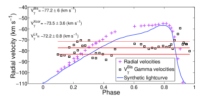
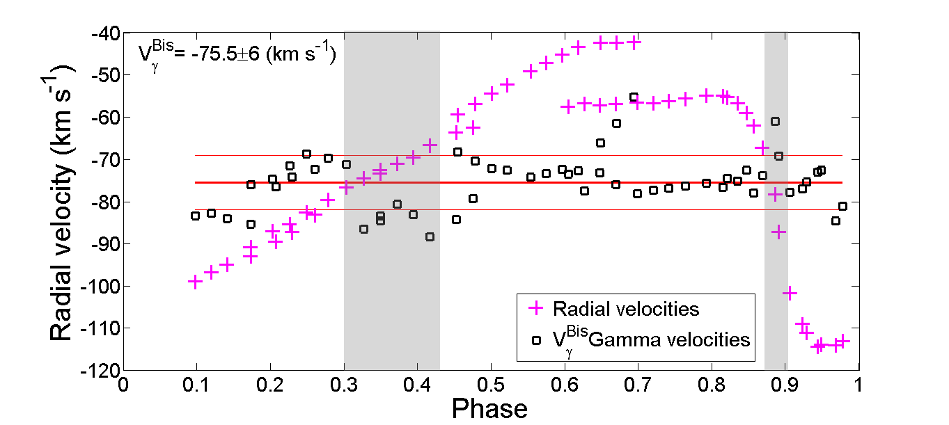
Figure 6: Top panel: gamma velocities of RR Lyr for non Blazhko phases derived using the method of bisectors (black squares), inferred from radial velocities measurements (magenta crosses) at different phases. The template radial velocity curve of RR Lyrae that was using for Xcor method is drawn as a blue solid line. Bottom panel: the same as previous including the Blazhko phases. Grey regions presumably corresponds to the phases with a low pulsation velocities, that does not affect the line profile asymmetry.

We finally derived an average value of $V_{\gamma}^{Bis}=-73.9\pm 5.9~{}km~{}s^{-1}$. This value is in agreement with literature references obtained with very high quality data, e.g. $V_{\gamma}^{RRLyr}=-72.0\pm 0.5~{}km~{}s^{-1}$ (Chadid, 2000). However, in the phase ranges 0.2–0.3 and 0.85–0.90, deviations up to 18 km s^-1 were found (grey shaded areas in Figure 6). In these phase ranges, the pulsational velocity is small, and our method is not very sensitive to $|v_{puls}|<5$ km s^-1 as it will be discussed in the next subsection. Moreover, strong shocks occur in RR Lyrae’s atmosphere at phases 0.85-0.9, contributing to the shape of line profiles, and those phases appear indeed to provide worse performances.

In order to test how flexible the bisectors method is, we derived the gamma velocities for RR Lyr with individual sets of bisectors grid for each observation, comparing it with gamma velocities derived using just one bisector grid for all observations. For this test we chose one bisector grid number 087 which corresponds to the phase 0.173 from our RR Lyrae synthetic models (see Table 4). In Figure 7, we present the pulsational velocities derived for each spectrum of RR Lyr obtained considering individual grids of bisectors and one grid of bisector (ID number 087). The average difference in pulsational velocities along the pulsation curve is relatively small ($<3~{}km~{}s^{-1}$), thus we can conclude that the use of only one bisector grid will not affect much the final gamma velocity estimations.

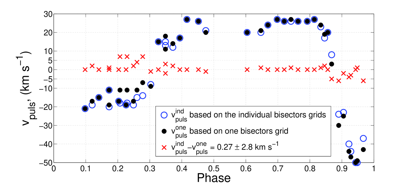
Figure 7: The difference between pulsational velocities for each spectrum of RR Lyr derived with the individual sets of bisectors grid and one grid of bisectors number 087 for all observed spectra.

Worth to discuss about one important ingredient, that has a significant impact on the analysis, is the microturbulent velocity; different authors (Kolenberg et al., 2010; Fossati et al., 2014) found the need of a depth-dependent value of microturbulence, varying with optical depth in the stellar atmosphere. To take the effect into account, we used the trend found by Fossati et al. (2014) to compute our synthetic spectra. The behaviour of bisector asymmetries computed with depth-dependent $v_{mic}$ stellar atmosphere models and with constant $v_{mic}$ atmosphere models is shown in Figure 8. As a constant $v_{mic}$ value, we adopt $v_{mic}=2~{}km~{}s^{-1}$, following Paper 1. The difference in residual asymmetries is rather large and, as a result, the difference in derived gamma velocities for each individual observation is significant (bottom panel of Figure 8). It is worth to notice that by using stellar atmosphere models with a depth-dependent microturbulent velocity the residual accuracy of the derived gamma velocity for RR Lyr is much smaller ($V_{\gamma,RRLyr}^{Bis,~{}depth-dep.~{}v_{mic}}=-80.2\pm 7.8~{}km~{}s^{-1}$) than the accuracy of the derived gamma velocity based on models with constant $v_{mic}$ ($V_{\gamma,RRLyr}^{Bis,~{}constant~{}v_{mic}}=-73.9\pm 5.9~{}km~{}s^{-1}$). We can conclude, that the current models of depth-dependent microturbulent velocity are not able to reproduce the real observed behaviour of the line profile asymmetries and the effect of depth dependent microturbulence velocity requires further theoretical investigations. Our analysis suggests that the use of grids of bisectors based on stellar atmospheres with constant $v_{mic}$ velocity should be preferred.

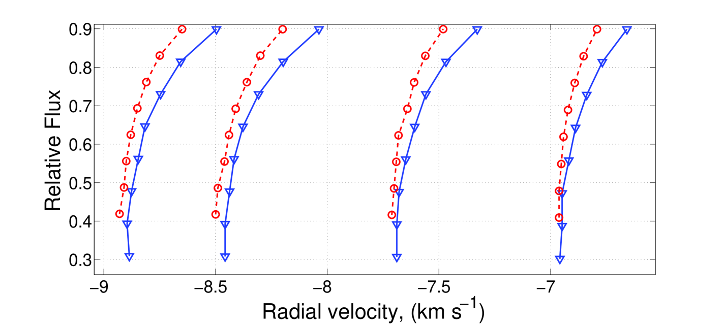
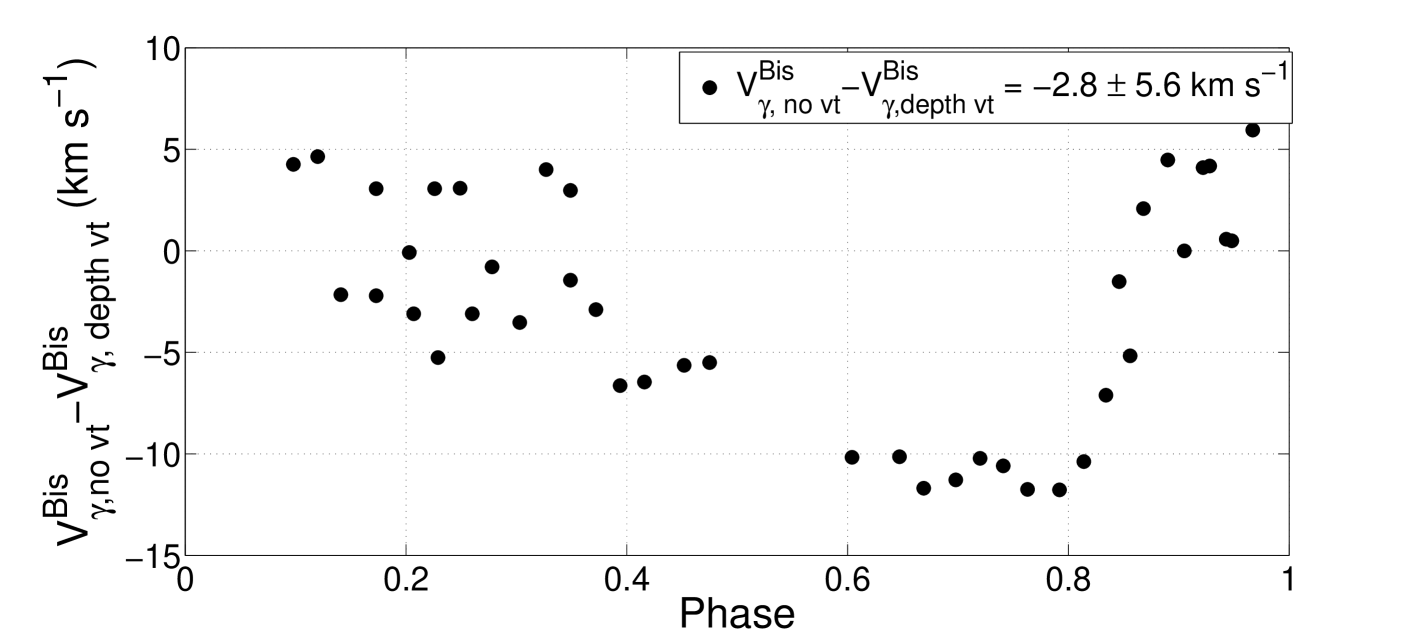
Figure 8: Top panel. Comparison of synthetic bisectors computed with the depth-dependent microturbulent velocity model (blue triangles) and with the constant microturbulent velocity $v_{mic}=2~{}km~{}s^{-1}$ (red circles). Bottom panel. The difference between the gamma velocities of RR Lyr derived with different sets of bisectors grid: with ($V_{\gamma}^{Bis,~{}depth-dep.~{}v_{mic}}$) and without depth-dependent $v_{mic}$ stellar atmosphere models ($V_{\gamma,RRLyr}^{Bis,~{}constant~{}v_{mic}}$).

4.4 The accuracies comparison of the bisectors method and the method of radial velocity curve template.

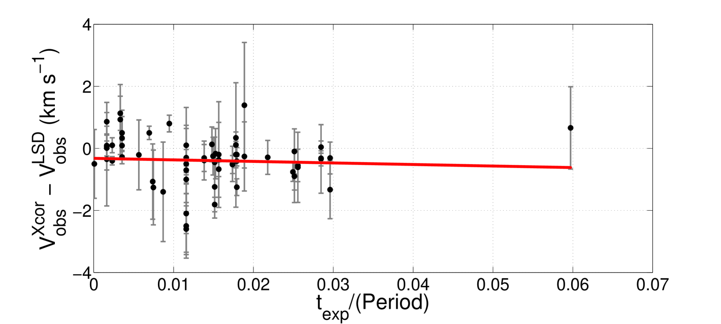
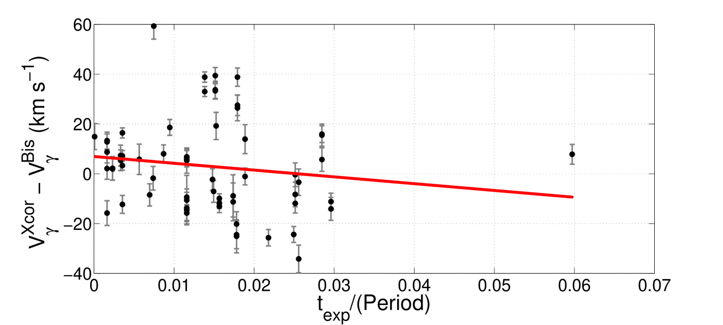
Figure 9: Difference between radial velocities (top panel) and gamma velocities (bottom panel) computed using the cross correlation method and method of bisectors as a function of exposure time of observed spectra. The red line in each plot corresponds to the linear fits of investigated values.

One source of uncertainty in this method is that observed spectra are usually taken with finite integration times, that cover a range of phases. The higher the spectral resolution of the observations, the longer the time needed to obtain a good S/N ratio, and the larger the phase smearing effect on the observed profile. The use of 4 or 8 m class telescopes alleviates the problem, but it is very difficult to avoid it completely, except for bright stars. The net result is a general broadening of the observed line profiles, compared to the theoretical ones. The smearing should cause subtle shifts in the minimum of the LSD profile — that should reflect on the derived $v_{obs}$ — and subtle changes in the line profile asymmetries — that should reflect on the derived $v_{puls}$. The size of these effects depends of course on the phase duration of the exposures. In our sample, we have exposures as long as 45 min (see Paper I), so we tested this hypothesis by comparing the difference between v_obs and V_γ obtained with the template curve method with those obtained with the bisectors method, and plotted them as a function of phase coverage in Figure 9. As can be seen, there is a hint that the bisectors method might slightly underestimate both velocities for increasing phase coverage, but the smearing effect — if any — does not affect much the individual errors of the observed radial velocity measurements. First of all, because when the phase smearing gets larger we do not see any significant trend in increasing the errors of observed and gamma velocities for the program stars. Thus, we can conclude that main sources of the individual errors in observed velocities have rather physical and instrumental (resolution and SNR) nature than the smearing effect. For the better understanding of this effect, it is necessary to perform the same analysis with simulated spectra for the given telescope and spectrograph which requires further studies.

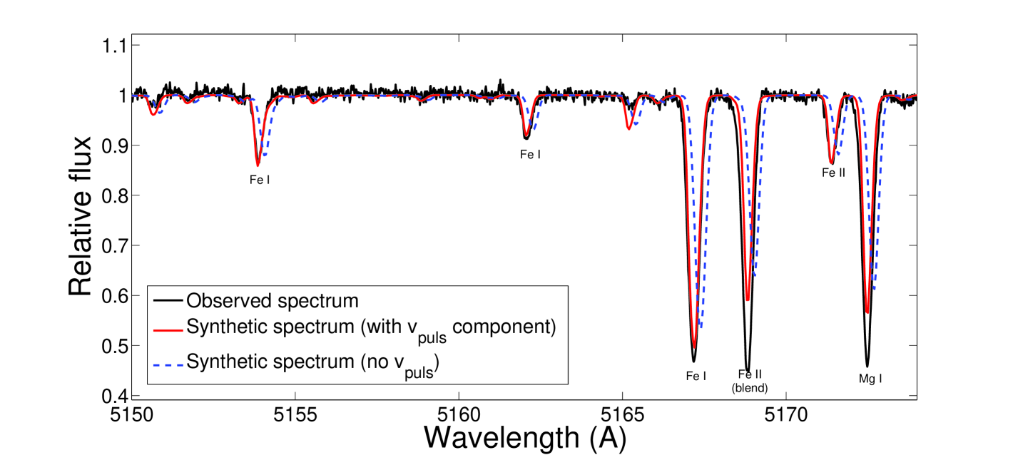
Figure 10: A portion of the spectrum of V Ind observed at phase 0.19 (black solid line) is superimposed to synthetic spectra with (red solid line) and without (blue dashed line) a pulsation velocity component. The synthetic spectra assume stellar parameters derived in Paper I, i.e. $T_{\mathrm{eff}}$ = 7000 K, $\log g=2.3$ dex, $v_{\mathrm{mic}}=1.6$ km s^-1. The pulsation velocity determined for this spectrum is $-17$ km s^-1.

Figure 10 illustrates the quality of our v_puls determinations: in spite of the large uncertainties involved in this kind of measurements, the addition of the v_puls component brings the synthetic and observed spectra in agreement. Moreover, it can be appreciated that the line shapes are different with and without inclusion of the pulsation velocity.

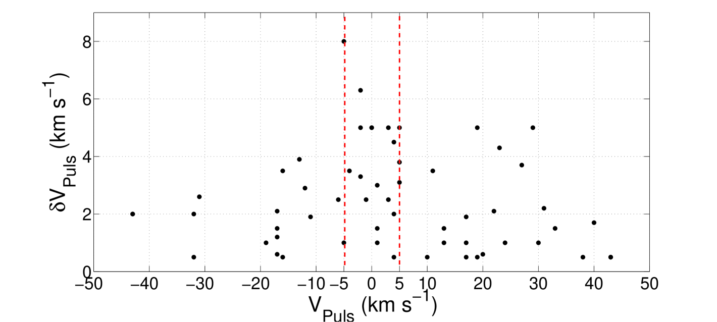
Figure 11: The errors on pulsational velocity (see text for details) for each observed spectrum at different pulsational velocities.

The resulting $v_{puls}^{Bis}$ determinations, with their errors $\delta v_{puls}^{Bis}$, are reported in Table 3, along with the final $V_{\gamma}$ and its propagated error, $\delta V_{\gamma}$. The errors on the pulsational velocity ($\delta v_{puls}^{Bis}$) have been computed as the standard deviation of measurements $v_{puls}^{Bis}$ obtained from the fit of different parts of the theoretical and observed bisectors, considering that LSD profiles can be distorted by blends. Thus, for each observation, we measured the pulsational velocities by using a different number of LSD profiles layers, namely we cut the bisectors at the fourth, fifth, sixth, and seventh layer, and derived a different v_puls for each cut. In this way, we tested how reliable bisectors are in reflecting the asymmetries of LSD profiles. The results are plotted in Figure 11, as a function of pulsational velocity of each individual exposure. As can be seen, the errors are always below 5 km s^-1, with a typical (median) value of 1.5 km s^-1, except for a narrow range of pulsational velocities, from –5 to +5 km s^-1, with a median value of 3.5 km s^-1. The comparably higher scatter that is obtained for pulsational velocities having smaller values is connected with the intrinsic sensitivity of the method: (i) blends do affect the shape of the LDS profile and (ii) the asymmetry of the profile tends to vanish for small pulsation velocities and consequently the error on its determination increases. This behavior of $\delta v_{puls}^{Bis}$ constrains the range of reliable application of the LSD method and has an impact on the gamma velocity error, $\delta V_{\gamma}$.

Figure 12 compares the final V_γ obtained with the classical and bisector methods. As can be seen, the stars that do not possess reliable observed curves in the literature (for example from the Baade-Wesselink method) have a larger difference, that is mostly caused by uncertainties in the classical template fitting method. If we limit the comparison to the stars having reliable template radial velocity curves, we can see an overall agreement at the level of $\Delta$V_γ=–0.1$\pm$10.7 km s^-1.

We also note that the most discrepant stars (marked in grey in Figure 12) are observed with SARG, and generally have lower S/N ratios and a larger phase coverage (smearing), because it is mounted on a 4 m-class telescope, while the UVES spectra produce less scattered results.

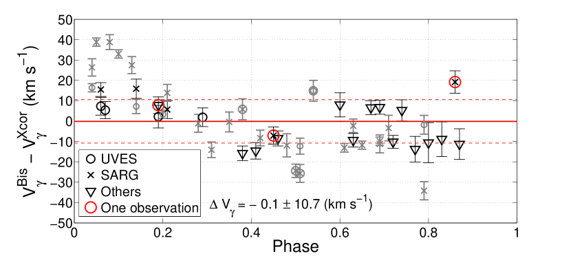
Figure 12: Difference between gamma velocities derived with the radial velocity curve template ($V_{\gamma}^{Xcor}$) and with the LSD profile asymmetry method ($V_{\gamma}^{Bis}$). The observations from the different spectrographs are labeled respectively, and stars that have only one epoch spectrum are also marked. Stars marked in black are those having reliable observed radial velocity curves in the literature (e.g., from the Baade-Wesselink method), while stars marked in grey have $V_{\gamma}^{Xcor}$ derived from less reliable templates.

Another way to study a posteriori the error on the whole method consists in evaluating the spread on repeated $V_{\gamma}$ measurements for the same star, when more than one determination was available. We found a typical spread of –10 to +10 km s^-1, with the maximum variations corresponding generally to the phase ranges 0.4–0.5. Figure 13 shows the difference of $V_{\gamma}$ measurements obtained from individual exposures with the average $V_{\gamma}$ of each star, as a function of phase. No systematic trends are apparent and the spread is generally consistent with the estimated errors.

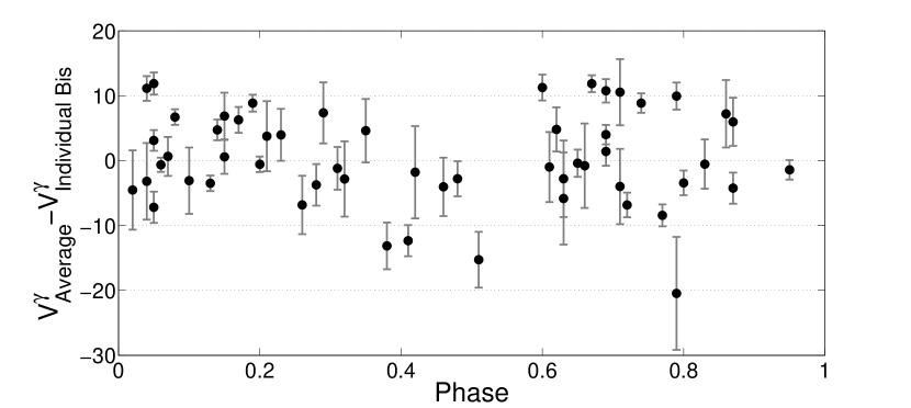
Figure 13: The difference of $V_{\gamma}^{Bis}$ of individual exposures with the average $V_{\gamma}$ for each star as a function of phase.

4.5 Projection factor

When deriving radial velocities from absorption line profiles, either with cross-correlation or with LSD profiles, the information is implicitly integrated over the stellar surface and along the radius of the pulsating star. Such integration is affected by limb darkening, across the stellar surface, and by radial velocity gradients with depth in the atmosphere of the star, where lines form. Both effects depend on the pulsation phase (Marengo et al., 2003), and therefore they are generally modeled as:

$$p=v_{puls}/(v_{rad}-V_{\gamma})\qquad(2)$$

also known as projection factor, or the factor by which one should multiply the observed radial velocity (in the line of sight) to obtain the intrinsic pulsational velocity of the star (along the radial direction), corrected by projection effects.

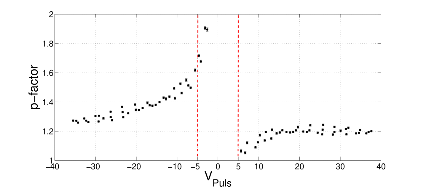
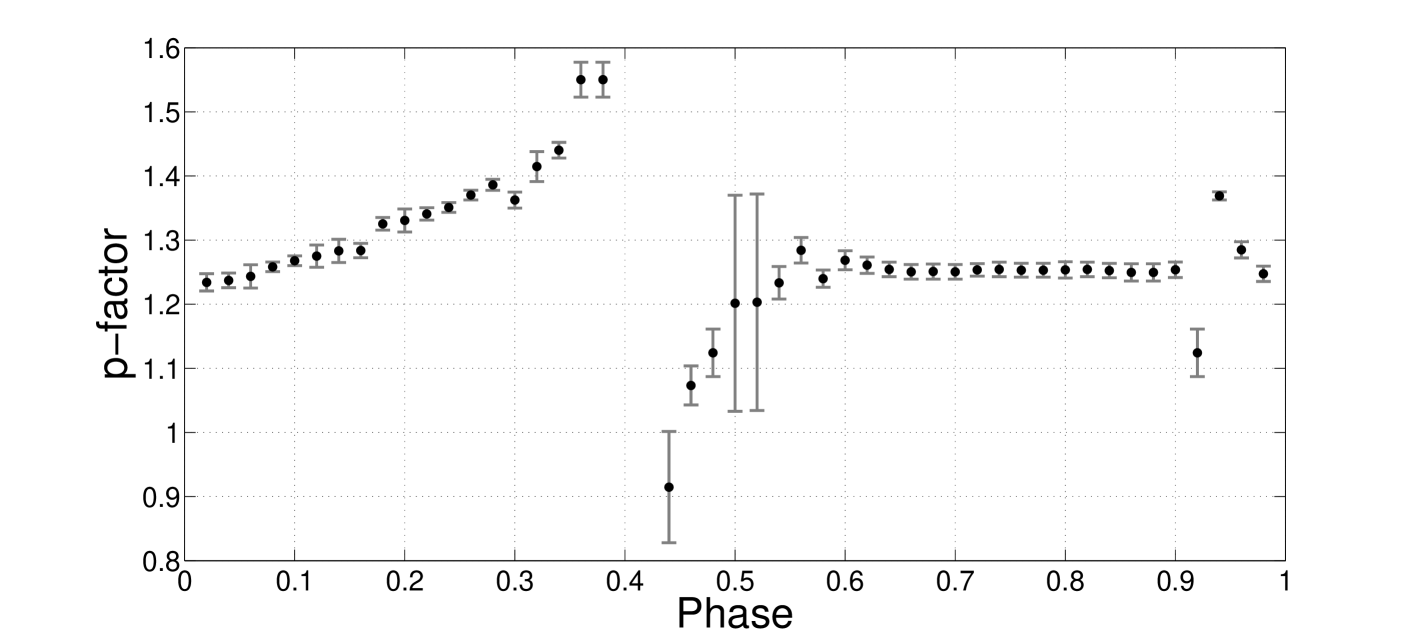
Figure 14: Model behavior of p-factor with different pulsation velocity (top panel) and different phases (bottom panel). We plotted the average values of the projection factor for each value of the modelled pulsational velocity, over all 41 bisector grids (see Appendix A). The vertical red dashed lines in the top panel mark the limits of applicability of our method (from –5 to +5 km s^-1, see also Figure 11), that roughly correspond to the phase range 0.35-0.50.

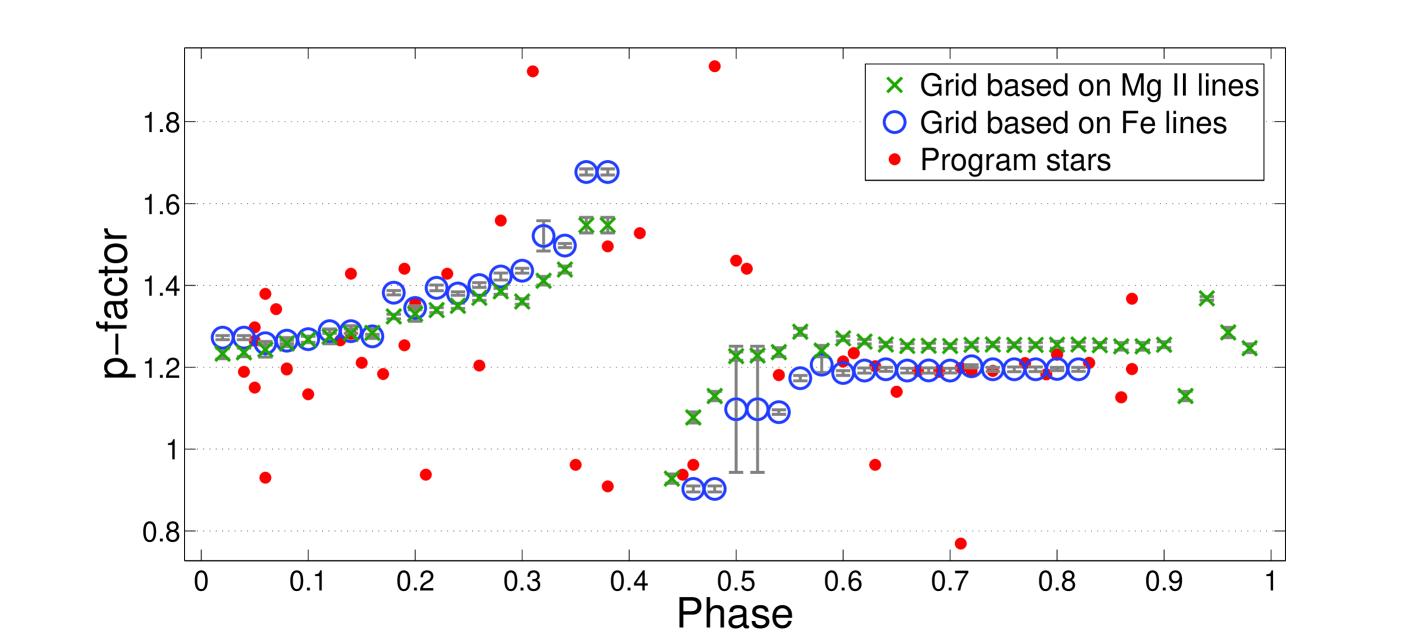
Figure 15: Observed behavior of p-factor with different phases for a sample of program spectra (red dots). As a reference the theoretical values of p-factor are labeled by blue circles and green crosses, which are based on the LSD profiles of synthetic spectra for all lines in the range 5100–5400 Å(blue circles) and the Mg I triplet lines only (green crosses).

The projection factor becomes very important in the Baade-Wesselink method, where a relatively small error in pulsation velocity may lead to a large error in distance. The first works by Eddington (1926) or Carroll (1928) lead to an estimate of $p=1.41$ that was used in many Baade-Wesselink studies of Cepheids, to correct for limb darkening and radial velocity expansion effects on the derived distances. Later, different values were proposed, ranging from 1.2 to 1.4 (see Nardetto et al., 2014, for a review). For the closest stars, it is possible to measure the projection factor directly, with the help of interferometric observations (e.g. Breitfelder et al., 2015). An investigation with realistic hydrodynamical models of $\delta$ Cep by Nardetto et al. (2004, see also the subsequent work by , and ) showed that projection effects can be corrected with residuals below $\simeq$1 km s^-1 and that the appropriate projection factor depends on the method used to derive the projected pulsational velocity.

In our case, the projection factor was computed using the bisectors method (an application to Cepheids can be found in Sabbey et al., 1995). We modeled the theoretical line profiles by taking into account the geometrical effect (limb darkening) for each model that we have used for calculations in our library of bisectors. The particularity of our approach is that we are using the average profiles of different spectral lines (via LSD technique) in order to investigate the clear geometrical effect of radial pulsations.

More in detail, we used the 41 existed models for RR Lyrae over all pulsation phases from Fossati et al. (2014). See Appendix A for more details. For each model, corresponding to a different phase, we computed a set of synthetic spectra with pulsation velocities ranging from -50 km s^-1 to +50 km s^-1 with a step of 1 km s^-1, in the same wavelength range used for our $v_{obs}$ measurements, 5100–5400 $\AA$ (see Figure 4). We then computed $v_{obs}$ and v_puls, as done on the observed spectra in our sample. We could then compute the projection factor using equations (1) and (2). In Figure 14, we illustrate the behavior of our modeled p-factor — obtained from our grids of model bisectors (Appendix A) — versus pulsational velocity and phase. The top panel clearly shows the limits of applicability of the bisectors method, which looses sensitivity in the -5 km s^-1 to +5 km s^-1 range, as discussed also previously. As a comparison, we repeated the same analysis using just the Mg I triplet lines (5167.321, 5172.684, 5183.604 $\AA$) instead of the all prominent lines from our initial linelist. In this case we built the synthetic grid of bisectors, and we derived the observed ones of our stellar sample, based only on these three lines. The Mg triplet is a prominent feature in the spectra of RR Lyraes, and it allowed us to test our p-factor modelization under different conditions (less numerous but stronger lines, see Figure 15).

In order to investigate the behavior of the projection factor on the sample of our real stars, we repeated the same procedure to derive the p-factor on the observed LSD profiles for the whole sample of stars. We can also plot the observed p-factor for each of the analyzed spectra, illustrated in Figure 15. Considering that we used the same bisectors library, we would expect to obtain roughly the theoretical behavior illustrated in the lower panel of Figure 14, modulated by the fitting uncertainties. While globally this is true, there are several outliers, that we can see in Figure 15, displaying in some cases totally unrealistic values of the p-factor, for example $p$$<$1 and $p$$>$1.6. This is most likely caused by measurement uncertainties in the derived v_puls, caused by line smearing, low S/N, blends, and other observational effects, and discussed in the previous section. But the overall behavior of p-factors derived from the observed profiles of our sample stars appears to agree well with that obtained from the models based on RR Lyrae. This confirms the overall self-consistency of our analysis. The comparisons of p-factors derived from our whole line list and from the Mg triplet shows a small offset that varies with phase (up to 0.07). We conclude that line selection can have a noticeable impact on the actual p-value derivation. When the offset is compared with the v_obs spread, however, it becomes largely irrelevant.

It should be noted, in the framework of our analysis we assume that all lines even with a different individual depths are behaving in the same way – i.e. the shape of all spectral features is the same at given pulsational velocity. This is not a fully correct assumption, however, the primary goal of this paper is to develop a method which can give reliable estimations of the gamma- and pulsational velocities just from one spectral observation. For this reason, using a few prominent lines or the list of many weak lines is equally good for deriving investigated velocities.

Table 5: Final results for the program stars, obtained with both the cross-correlation and the bisectors methods.

Star	$V_{\gamma}^{Xcor}$	$\delta V_{\gamma}^{Xcor}$	$V_{\gamma}^{Bis}$	$\delta V_{\gamma}^{Bis}$
	(km s-1)	(km s-1)	(km s-1)	(km s-1)
DR And	–119	9	–110	4
X Ari*	–36	5	–44	6
TW Boo	–100	2	–89	2
TW Cap*	–72	6	–87	6
RX Cet*	–94	5	–68	6
U Com	–7	4	–19	6
RV CrB	–140	4	–133	5
UZ CVn	–18	4	–49	6
SW CVn	21	7	14	6
AE Dra	–276	2	–311	5
BK Eri	97	4	93	11
UY Eri*	152	6	146	7
SZ Gem*	322	5	346	6
VX Her	–371	5	–352	10
DH Hya	334	5	348	18
V Ind	197	3	200	9
SS Leo	164	5	157	2
V716 Oph*	–311	6	–370	6
VW Scl	40	4	36	13
BK Tuc	170	5	134	7
TU UMa*	99	5	106	7
RV UMa	–198	5	–175	6
UV Vir*	99	5	81	6

Note. * For these stars only one spectrum was obtained.

5 Discussion

The final velocity measurements for each star, measured with the two methods, were obtained as averages of the single-epoch gamma determinations listed in Tables 2 and 3, respectively, and they are listed in Table 5 along with their errors. The comparison between the two methods was already discussed in Section 4 (see Figures 9 and 12). Here, we will compare our results with the available literature. We will also discuss more in depth the uncertainties and applicability of the bisectors method to the derivation of gamma velocities for pulsating stars.

Table 6: Summary of literature results on the program stars, for both the observed heliocentric radial velocity estimates ($v_{rad}$) and the gamma velocities (V_γ), along with their errors, when available.

Star	$v_{rad}^{Lit}$	$\delta v_{rad}^{Lit}$	Ref	$V_{\gamma}^{Lit}$	$\delta V_{\gamma}^{Lit}$	Ref
	(km s-1)	(km s-1)		(km s-1)	(km s-1)
DR And	–81	30	(1)	–103.6	2.0	(3)
X Ari*	–36	1	(1)	–41.6	3	(4)
TW Boo	–99	1	(1)	–99	5	(5)
TW Cap	–32	1	(1)	…	…
RX Cet	–57	2	(1)	…	…
U Com*	–22	3	(1)	–18	3	(6)
RV CrB	–125	5	(1)	–125	5	(7)
UZ CVn*	–28	3	(1)	–27	10	(6)
SW CVn	–18	21	(1)	–18	21	(8)
AE Dra	–243	30	(1)	–243	30	(8)
BK Eri	141	10	(1)	141	10	(7)
UY Eri	171	1	(1)	…	…
SZ Gem	326	4	(1)	305	15	(5)
VX Her*	–377	3	(1)	–361.5	5	(4)
DH Hya	355	8	(1)	355	8	(7)
V Ind*	202	2	(1)	202.5	2	(9)
SS Leo*	144	7	(2)	162.5	6.8	(10)
V716 Oph	–230	30	(1)	–230	5	(11)
VW Scl	53	10	(1)	53	10	(12)
BK Tuc	121	14	(1)	121	14	(7)
TU UMa*	89	2	(1)	101	3	(13)
RV UMa	–185	1	(1)	–185	1	(7)
UV Vir	99	11	(1)	99	11	(7)

Notes. * These stars were studied with the Baade-Wesselink method. Literature references: (1) Beers et al. (2000); (2) Kordopatis et al. (2013); (3) Jeffery et al. (2007); (4) Nemec et al. (2013); (5) Hawley & Barnes (1985); (6) Fernley & Barnes (1997); (7) Dambis (2009); (8) Layden (1994); (9) Clementini et al. (1990); (10) Carrillo et al. (1995); (11) McNamara & Pyne (1994); (12) Solano et al. (1997); (13) Preston & Spinrad (1967).

5.1 Literature comparisons

We report in Table 6 our literature search for radial and gamma velocity measurements of the program stars (V${}_{\gamma}^{Lit}$). We compare the gamma velocities obtained in the literature with our measurements obtained with both methods in Figure 16. As can be seen, both the classical method (top panel) and the bisector method (bottom panel) produce results that are generally compatible with the literature, within the quoted uncertainties, with a few exceptions.

We note that for the most discrepant cases, like AE Dra, UZ CVn, or BK Eri, the discrepancy with the literature persists regardless of the method employed, suggesting that maybe there is a problem with those specific stars. The spectra of SW CVn and RV CrB have low S/N ratio ($\leq$50) and they were excluded from the abundance analysis in Paper I, however, we included them in this work, because the S/N ratio was sufficient for radial velocity analysis. These stars were included here because the S/N ratio was sufficient to produce reliable radial velocity estimates, and indeed they agree with the literature with both methods. The spectra of AE Dra have good S/N ratios but they suffer from some phase smearing because they were observed for 30 and 45 minutes and this is reflected in their large error bars, which make them only marginally incompatible with the literature. The spectra of BK Eri have quite high S/N and short exposure times, so we suspect that in that case the problem might lie in the literature measurements. Finally, there are two stars that show marginally discrepant values with the literature, and from one method to the other: SZ Gem and BK Tuc. SZ Gem has only one spectrum and this can pose a problem of non reliable template curve fitting or non sensitive regime of pulsation phases in the bisectors method – between –5 km s^-1 and +5 km s^-1. Indeed, the derived pulsational velocity for this spectrum is relatively small 13 km s^-1 at phase 0.50. BK Tuc was observed in three exposures of 30 min each, which might introduce some phase smearing of the line profiles.

If we exclude the three most problematic stars, both methods compare quite well with the literature, with the following weighted average differences: $\Delta$V${}_{\gamma}^{Xcor}$=–3$\pm$20 km s^-1 and $\Delta$V${}_{\gamma}^{Bis}$=–3$\pm$30 km s^-1, where the differences are computed as our measurements minus the literature ones. The observed spreads are marginally incompatible with the typically quoted uncertainties, which are of 5, 12, and 7 km s^-1 for the cross-correlation method, the bisectors method, and the literature collection, respectively. The uncertainties quoted for the different methods are rather compatible with each other, suggesting that there must be some error source that has been unaccounted for in all of the methods. If so, the unaccounted-for error source amounts to 10–20 km s^-1 in each method. Systematic errors of this amplitude are easy to accommodate when one applies the template curve fitting to just a few measurements as in our case. These errors are also easy to accommodate, at least for the noisiest spectra, into the bisectors method sensitivity. On the other hand, we are comparing with literature results that are derived with several different methods and data samples, so the inhomogeneity of the comparison measurements certainly plays an important role. Explanation of this general spread in comparison of gamma velocities with the literature values, likely can be found in the fact that the stars for which the B-W analysis was performed have a difference in this comparison less than or equal to 10  km s^-1 in both V${}_{\gamma}^{Xcor}$ - V${}_{\gamma}^{Lit}$ and V${}_{\gamma}^{LSD}$ - V${}_{\gamma}^{Lit}$ values. It is a rather small difference, and the reason for this is actually that these stars have reliable radial velocity curves based on the B-W method. As a result the V${}_{\gamma}^{Xcor}$ are more reliable as well, because the light curve analysis was based on the same radial velocity curves as in the B-W method. Moreover, in Figure 12 we can see the same behavior of difference V${}_{\gamma}^{Xcor}$ - V${}_{\gamma}^{LSD}$ – the stars for which the B-W method was applied in the literature, have less scatter in the gamma velocity.

We can conclude, after considering the literature comparison with stars having reliable radial velocity curves, that the bisector’s method performs at least as well as the more traditional template curve technique.

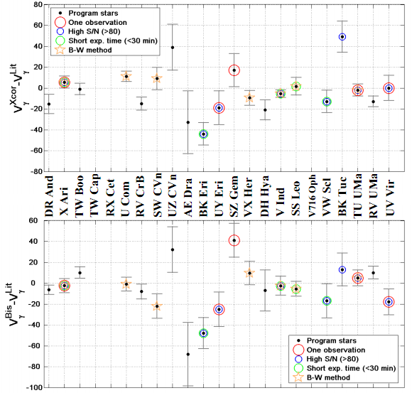
Figure 16: Differences between our measurements and literature ones. Top panel: difference between gamma velocities from cross-correlation method and template curve fitting (V${}_{\gamma}^{Xcor}$) with the literature (V${}_{\gamma}^{Lit}$). Bottom panel: difference between the gamma velocity from LSD profiles and bisectors (V${}_{\gamma}^{LSD}$) with the literature. We marked the stars by different colors taking into account some relevant characteristics of their spectra: the stars that have only one measurement (red), short exposure times (green), high SNR (blue), and Baade-Wesselink literature estimates (orange).

6 Conclusions

We perform a systematic study of the radial velocities for a sample of 23 variable stars – mostly RRab, with two RRc and three W Vir – using high-resolution spectra from both proprietary (UVES and SARG) and archival (UVES, HARPS, FEROS, APO) data sets.

For each star, we derive the radial velocity using two independent methods: the cross-correlation approach and the LSD profile technique. The errors of individual estimates of radial velocity in both methods are on the level $\pm~{}2~{}km~{}s^{-1}$, or less. The determination of gamma velocities was also performed with two methods, the first based on the classical radial velocity curve template technique and the second on the line profile asymmetries, referred to as the bisectors method (see Section 4.2). With the help of LSD technique we provide and test a method for determining the pulsation and gamma velocity of pulsating variable stars when only scarce observations taken at random phases are available. We also computed a grid of synthetic bisectors for each of 41 phases (see Appendix A), that is made available electronically. Our public library can be used in general case to make an assumptions about velocity of barycenter of pulsating stars, in best case within error $\pm~{}5~{}km~{}s^{-1}$.

In summary this work, the presented method of deriving gamma velocities of RR Lyraes has the next milestones:

1. the method is working well for the radially pulsating stars: RRab Lyraes, classical Cepheids; to quantify the level of line profile asymmetry, we used the average profile of different spectral lines (the LSD profile);

2. the method is phase sensitive, the best accuracy of derived at phases 0 – 0.2 and 0.5 – 0.85; at these phases the pulsation velocity is large, thus the line profile asymmetry is more easy to identify;

3. the shock phases during the pulsation cycle in RRab stars do affect the accuracy of the method mostly on phases 0.85 – 0.95, when the line profile geometry changes dramatically;

4. the method is working with both low- and high- S/N spectra, the spectra resolution at which we applied the method was about $R\approx 30000$;

5. the major advantage is that it can derive the gamma velocity of a star just from one observation, or from observations taken at unknown phase, however, the accuracy of the method depends on many factors, we estimated the average error of determined pulsational velocity is $\delta$$v_{puls}$ $\approx$ 3.5 km s^-1 and the residual error of gamma velocity is $\delta$V${}_{\gamma}^{Bis}$ $\approx$ 10 km s^-1.

Appendix A Grids of synthetic bisectors.

We publish a grid of synthetic bisectors, that can be used to compute the pulsational velocity of any observed spectrum of radial pulsating variables of the RRab Lyrae type and Cepheids with the method described in Section 4. Due to the small number of RRc variables (only 2) in our sample we could not make statistically significant conclusions about the method application to this type of variables. The grid contains one set of bisectors (from $-50$ to $+50~{}km~{}s^{-1}$ with a step $1~{}km~{}s^{-1}$ of pulsational velocity variation) for each of the 41 different phases computed on the basis of the individual atmospheric models along the pulsation cycle of RR Lyr. Each individual atmospheric model was based on the stellar parameters derived in Fossati et al. (2014) and phase coverage is presented in the Table 4. The IDs of each bisector grid correspond to the IDs of the atmospheric models from Fossati et al. (2014).

In order to build the grid of bisectors, we were following the next steps. For each of the 41 selected phases we computed a set of synthetic spectra in the same wavelength range used for the radial velocity measurements (5100–5400 Å) with the STARSP-SynthV code (Tsymbal, 1996), based on the ATLAS9 model atmospheres. We used the last modification of the code that for the construction of line profiles took into account the stellar radial pulsations, individual chemical abundances, and depth-dependent microturbulent velocity for a given star. For the calculations, we adopt a constant microturbulent velocity of $2~{}km~{}s^{-1}$ . However, as discussed at the end of subsection 4.3, the choice of one bisector grid for the analysis of all observed spectra will have no effect on the accuracy of the final gamma velocity measurements. For each synthetic spectrum, we computed the LSD profile and its bisector, using exactly the same method adopted for the observed spectra (Section 4). The resulting sets of bisectors serve us as a final library of bisectors.

Table 7: The grids of synthetic bisectors. The names of the files correspond to the spectrum ID of that phase by Fossati et al. (2014). The columns contain: (1) the intrinsic pulsational velocity $v_{puls}$ of the bisector points; (2) the difference $v_{rad}-V_{\gamma}$, or in other words the observed pulsational velocity uncorrected for projection effects, see the equation (2); (3-10) the X_n coordinates of the eight bisector points, or in other words the centers of the bisectors in radial velocity space, expressed as offsets from the gamma velocity (zero by definition, in this system); (11-18) the Y_n coordinates of the eight bisector points, expressed in relative flux (where 1 is the continuum and 0 full absorption); and (19) the Full Width at Half Maximum of the synthetic LSD profile (see text). The table is available in its entirety on the electronic version of the Journal, and at CDS. Only the first five rows are reported here, for guidance about its form and contents.

$v_{puls}$	$v_{rad}-V_{\gamma}$*	X1	…	X8	Y1	…	Y8	FWHM
km s-1	km $s^{-1}$	km s-1	…	km s-1	(%)	…	(%)	$\AA$
–45	–35.43	0.32	…	3.53	0.67	…	0.91	23.30
–44	–34.65	0.37	…	3.49	0.66	…	0.91	22.92
–43	–34.21	0.42	…	4.24	0.68	…	0.91	23.90
–42	–32.67	0.29	…	3.56	0.67	…	0.91	23.06
–41	–32.25	0.27	…	3.62	0.65	…	0.91	21.78

Notes. * The accuracy in estimation of observed synthetic pulsational velocities ($v_{rad}-V_{\gamma}$) corresponds to the accuracy of finding minimum of the appropriate LSD profile (i.e. $\delta v_{obs}^{LSD}$), see the Section 4.1.

The grid is published in the electronic version of the Journal and in CDS, and Table 7 provides an example of its contents. To be able to use the grid, the set with the phase closest to the observed one needs to be selected, and then the bisector’s points need to be scaled to the actual resolution of the observed spectra, by multiplying the X_n coordinates of the eight bisector points by

$$\frac{FWHM_{LSD}}{FWHM_{obs}}$$

where FWHM_LSD is the Full-Width at Half Maximum of the synthetic bisector, reported in the last column of Table 7, while FWHM_obs is the one obtained for the observed spectra.

General suggestion is that to make more accurate determination of center-of-mass velocity of radial pulsating Cepheids and RR Lyrae it is better to use individual grids of synthetic bisectors. Since the line profile asymmetry depends on atmospheric parameters, in ideal situation it is necessary to build the grid of synthetic spectrum with $T_{eff}$, $log~{}g$ and $v_{mic}$ for a particular star, but the provide values can be used for stars that are not too different from RR Lyrae.

References

- Ballester et al. (2000) Ballester P., Modigliani A., Boitquin O., Cristiani S., Hanuschik R., Kaufer A., Wolf S., 2000, The Messenger, 101, 31
- Beers et al. (2000) Beers T. C., Chiba M., Yoshii Y., Platais I., Hanson R. B., Fuchs B., Rossi S., 2000, AJ, 119, 2866
- Benedict et al. (2011) Benedict G. F., McArthur B. E., Feast M. W., Barnes T. G., Harrison T. E., Bean J. L., Menzies J. W., Chaboyer B., Fossati L., et al., 2011, AJ, 142, 187
- Breitfelder et al. (2015) Breitfelder J., Kervella P., Mérand A., Gallenne A., Szabados L., Anderson R. I., Willson M., Le Bouquin, J.-B., 2015, A&A, 576, A64
- Cacciari et al. (1989) Cacciari, C., Clementini, G., Prevot, L., & Buser, R., 1989, A&A, 209, 141
- Cacciari et al. (1987) Cacciari, C., Clementini, G., Prevot, L., et al., 1987, AJ, 69, 135
- Cacciari & Clementini (2003) Cacciari C., Clementini G., 2003, Berlin Springer Verlag, 635, 105
- Carrillo et al. (1995) Carrillo D., Burki G., Mayor M., Burnet M., Lampens P., Nicolet B., 1995, A&AS, 113, 483
- Carroll (1928) Carroll J. A., 1928, MNRAS, 88, 548
- Chadid (2000) Chadid M., 2000, A&A, 359, 991
- Chadid et al. (2008) Chadid M., Vernin J., Gillet D., 2008, A&A, 491, 537
- Clementini et al. (1990) Clementini, G., Cacciari, C., & Lindgren, H., 1990, A&A, 85, 865
- Dambis (2009) Dambis A. K., 2009, MNRAS, 396, 553
- Dekker et al. (2000) Dekker H., D’Odorico S., Kaufer A., Delabre B., Kotzlowski H., 2000, SPIE, 4008, 534
- Donati et al. (1997) Donati J.-F., Semel M., Carter B. D., and Rees D. E., Collier Cameron A., 1997, MNRAS, 291, 658
- Eddington (1926) Eddington A. S., 1926, ics..book,
- Fernley & Barnes (1997) Fernley J., Barnes T. G., 1997, A&AS, 125, 313
- For et al. (2011) For B.-Q., Sneden C., Preston G. W., 2011, ApJS, 197, 29
- Fossati et al. (2014) Fossati L., Kolenberg K., Shulyak D. V., Elmasli A., Tsymbal V., Barnes T. G. Guggenberger E., Kochukhov O., 2014, MNRAS, 445, 4094
- Gonzalez & Wallerstein (1996) Gonzalez G. & Wallerstein G. 1996, MNRAS, 280, 515
- Gratton et al. (2001) Gratton R. G., et al., 2001, ExA, 12, 107
- Gray (2010) Gray D. F., 2010, ApJ, 721, 670
- Guggenberger et al. (2014) Guggenberger E., Shulyak D., Tsymbal V., Kolenberg K., 2014, IAU, 301, 261
- Hareter et al. (2008) Hareter M., et al., 2008, A&A, 492, 185
- Harris & Welch (1989) Harris, H. C. & Welch, D. L., 1989, AJ, 98, 981
- Hatzes A. (1996) Hatzes A. P., 1996, PASP, 108, 839
- Hawley & Barnes (1985) Hawley S.L., Barnes III T. G., 1985, PASP, 97, 551
- Jeffery et al. (2007) Jeffery E. J., Barnes III T. G., and Skillen I., Montemayor T. J.,2007, ApJS, 171, 512
- Jones et al. (1987) Jones, R. V., Carney, B. W., Latham, D. W., & Kurucz, R. L., 1987, AJ, 312, 254
- Jones et al. (1988) Jones, R. V., Carney, B. W., & Latham, D. W., 1988, AJ, 326, 312
- Kochukhov et al. (2010) Kochukhov O., Makaganiuk V., Piskunov N., 2010, A&A, 524, A5
- Kollmeier et al. (2009) Kollmeier J. A., Gould A., Shectman S., Thompson I. B., Preston G. W., Simon J. D., Crane J. D., Ivezić Ž., Sesar B., 2009, ApJ, 705, 158
- Kolenberg et al. (2010) Kolenberg K., Fossati L., Shulyak D, Pikall H., Barnes T. G., Kochukhov O., Tsymbal, V., 2010, A&A, 519, A64
- Kordopatis et al. (2013) Kordopatis G., Gilmore G., Steinmetz M., Boeche C., Seabroke, G. M., Siebert A., Zwitter T., 2013, AJ, 146, 134
- Kurucz (1993) Kurucz R, 1993, CD-ROM No. 18. Cambridge, Mass.: Smithsonian Astrophysical Observatory, 18
- Layden (1994) Layden A. C., 1994, AJ, 108, 1016
- Liu & Janes (1989) Liu, T., & Janes, K. A., 1989, AJ, 69, 593
- Liu (1991) Liu, T., 1991, PASP, 103, 205
- Maas et al. (2007) Maas T., Giridhar S., Lambert D. L., 2007, AJ, 666, 378
- McNamara & Pyne (1994) McNamara D. H., Pyne M. D., 1994, PASP, 106, 472
- Marengo et al. (2003) Marengo M., Karovska M., Sasselov D. D., Papaliolios C., Armstrong J. T., Nordgren T. E., 2003, ApJ, 589, 968
- Moskalik et al. (2015) Moskalik P., Smolec R., Kolenberg K., Molnár L., Kurtz D. W., Szabó R., Benkő J. M., Nemec J. M. Chadid M., Guggenberger E., Ngeow C.-C., Jeon Y.-B., Kopacki G., Kanbur S. M., 2015, MNRAS, 447, 2348
- Mucciarelli et al. (2013) Mucciarelli A., Pancino E., Lovisi L., Ferraro F. R., Lapenna E., 2013, ApJ, 766, 78
- Nardetto et al. (2004) Nardetto N., Fokin A., Mourard D., Mathias P., Kervella P., Bersier D., 2004, A&A, 428, 131
- Nardetto et al. (2008) Nardetto N., Stoekl, A., Bersier D., Barnes T.G., 2008, A&A, 489, 1255
- Nardetto et al. (2013) Nardetto N., Mathias P., Fokin A., Chapellier E., Pietrzynski G., Gieren W., Graczyk D., Mourard D., 2013, A&A, 553, A112
- Nardetto et al. (2014) Nardetto N., Poretti E., Rainer M., Guiglion G., Scardia M., Schmid V. S., Mathias P., 2014, A&A, 561, A151
- Nardetto et al. (2014) Nardetto N., Storm J., Gieren W., Pietrzyński G., Poretti E., 2014, IAU Symposium, 301, 145-148
- Nardetto et al. (2017) Nardetto N., Poretti E., Rainer M., Fokin A., Mathias P., Anderson R. I., Gallenne A., Gieren W., Graczyk D., Kervella P., Mérand A., Mourard D., Neilson H., Pietrzynski G., Pilecki B., Storm J., 2017, A&A, 597, A73
- Nemec et al. (2013) Nemec J. M., Cohen J. G., Ripepi V., Derekas A., Moskalik P., Sesar B., Chadid M., Bruntt H., 2013, ApJ, 773, 181
- Pancino et al. (2015) Pancino E., Britavskiy N., Romano D., Cacciari C., Mucciarelli A., Clementini G., 2015, MNRAS, 447, 2404 (Paper I)
- Preston & Spinrad (1967) Preston G. W., Spinrad H., 1967, ApJ, 147, 1025
- Prusti (2014) Prusti T., 2014, acm..conf, 434
- Prusti et al. (2016) Gaia Collaboration, Prusti T., et al. 2016, A&A, 595, A1
- Sabbey et al. (1995) Sabbey C. N., Sasselov D. D., Fieldus M. S., Lester J. B., Venn K. A., Butler R. P., 1995, ApJ, 446, 250
- Kharchenko et al. (2007) Kharchenko N. V., Scholz R.-D., Piskunov A. E., Róser S., Schilbach E., 2007, Astronomische Nachrichten, 328, 889
- Sanford (1952) Sanford R. F., 1952, ApJ, 116, 331
- Samus et al. (2007) Samus N.N., Durlevich O.V., Kazarovets E V., Kireeva N.N., Pastukhova E.N., Zharova A.V., et al., General Catalogue of Variable Stars (Samus+ 2007-2012)
- Sessar (2012) Sessar B., 2012, AJ, 144, 114
- Skarka (2013) Skarka M., 2013, A&A, 549, A101
- Solano et al. (1997) Solano E., Garrido R., Fernley J., Barnes T. G., 1997, A&AS, 125, 321
- Stetson & Pancino (2008) Stetson P. B., Pancino E., 2008, PASP, 120, 1332
- Stetson et al. (2014) Stetson P. B., Fiorentino G., Bono G., Bernard E. J., Monelli M., Iannicola G., Gallart C., Ferraro I., 2014, PASP, 126, 616
- Szatmary (1990) Szatmary K., 1990, JAAVSO, 19, 52
- Tkachenko et al. (2013) Tkachenko A., Van Reeth T., Tsymbal V., Aerts C., Kochukhov O., Debosscher J., 2013, A&A, 560, A37
- Tonry & Davis (1979) Tonry J., Davis M., 1979, AJ, 84, 1511
- Tsymbal (1996) Tsymbal V. V. 1996, in Adelman S. J., Kupka F., Weiss W. W., eds, ASP Conf. Ser. Vol. 108, Model Atmospheres and Spectrum Synthesis. Astron. Soc. Pac., San Francisco, p. 198
- Van Reeth et al. (2013) Van Reeth T., Tkachenko A., Tsymbal V., 2013, EAS Publications Series, 64, 237
- Wallerstein (1958) Wallerstein G., 1958, ApJ, 127, 583