Variational Bi-LSTMs

Abstract

Recurrent neural networks like long short-term memory (LSTM) are important architectures for sequential prediction tasks. LSTMs (and RNNs in general) model sequences along the forward time direction. Bidirectional LSTMs (Bi-LSTMs) on the other hand model sequences along both forward and backward directions and are generally known to perform better at such tasks because they capture a richer representation of the data. In the training of Bi-LSTMs, the forward and backward paths are learned independently. We propose a variant of the Bi-LSTM architecture, which we call Variational Bi-LSTM, that creates a channel between the two paths (during training, but which may be omitted during inference); thus optimizing the two paths jointly. We arrive at this joint objective for our model by minimizing a variational lower bound of the joint likelihood of the data sequence. Our model acts as a regularizer and encourages the two networks to inform each other in making their respective predictions using distinct information. We perform ablation studies to better understand the different components of our model and evaluate the method on various benchmarks, showing state-of-the-art performance.

1 Introduction

Recurrent neural networks (RNNs) have become the standard models for sequential prediction tasks with state of the art performance in a number of applications like sequence prediction, language translation, machine comprehension, and speech synthesis (Arik et al., 2017; Wang et al., 2017; Mehri et al., 2016; Sotelo et al., 2017). RNNs model temporal data by encoding a given arbitrary-length input sequentially, at each time step combining a transformation of the current input with the encoding from the previous time step. This encoding, referred to as the RNN hidden state, summarizes all previous input tokens.

Viewed as “unrolled” feedforward networks, RNNs can become arbitrarily deep depending on the input sequence length, and use a repeating module to combine the input with the previous state at each time step. Consequently, they suffer from the vanishing/exploding gradient problem (Pascanu et al., 2012). This problem has been addressed through architectural variants like the long short-term memory (LSTM) (Hochreiter & Schmidhuber, 1997) and the gated recurrent unit (GRU) (Chung et al., 2014). These architectures add a linear path along the temporal sequence which allows gradients to flow more smoothly back through time.

Various regularization techniques have also been explored to improve RNN performance and generalization. Dropout (Srivastava et al., 2014) regularizes a network by randomly dropping hidden units during training. However, it has been observed that using dropout directly on RNNs is not as effective as in the case of feed-forward networks. To combat this, Zaremba et al. (2014) propose to instead apply dropout on the activations that are not involved in the recurrent connections (Eg. in a multi-layer RNN); Gal & Ghahramani (2016) propose to apply the same dropout mask through an input sequence during training. In a similar spirit to dropout, Zoneout (Krueger et al., 2016) proposes to choose randomly whether to use the previous RNN hidden state.

The aforementioned architectures model sequences along the forward direction of the input sequence. Bidirectional-LSTM, on the other hand, is a variant of LSTM that simultaneously models each sequence in both the forward and backward direction. This enables a richer representation of data, since each token’s encoding contains context information from the past and the future. It has been shown empirically that bidirectional architectures generally outperform unidirectional ones on many sequence-prediction tasks. However, the forward and backward paths in Bi-LSTMs are trained separately and the benefit usually comes from the combined hidden representation from both paths. In this paper, our main idea is to frame a joint objective for Bi-directional LSTMs by minimizing a variational lower bound of the joint likelihood of the training data sequence. This in effect implies using a variational auto-encoder (VAE; Kingma & Welling (2014)) that takes as input the hidden states from the two paths of the Bi-LSTM and maps them to a shared hidden representation of the VAE at each time step. The samples from the VAE’s hidden state are then used for reconstructing the hidden states of both the LSTMs. While the use of a shared hidden state acts as a regularizaer during training, the dependence on the backward path can be ignored during inference by sampling from the VAE prior. Thus our model is applicable in domains where the future information is not available during inference (Eg. language generation). We refer to our model as Variational Bi-LSTM. We note that recently proposed methods like TwinNet (Serdyuk et al., 2017) and Z-forcing (Sordoni et al., 2017) are similar in spirit to this idea. We discuss the differences between our approach and these models in section 5.

Below, we describe Variational Bi-LSTMs in detail and then demonstrate empirically their ability to model complex sequential distributions. In experiments, we obtain state-of-the-art or competitive performance on the tasks of Penn Treebank, IMDB, TIMIT, Blizzard, and Sequential MNIST.

2 Variational Bi-LSTM

Bi-LSTM is a powerful architecture for sequential tasks because it models temporal data both in the forward and backward direction. For this, it uses two LSTMs that are generally learned independent of each other; the richer representation in Bi-LSTMs results from combining the hidden states of the two LSTMs, where combination is often by concatenation. The idea behind variational Bi-LSTMs is to create a channel of information exchange between the two LSTMs that helps the model to learn better representations. We create this dependence by using the variational auto-encoder (VAE) framework. This enables us to take advantage of the fact that VAE allows for sampling from the prior during inference. For sequence prediction tasks like language generation, while one can use Bi-LSTMs during training, there is no straightforward way to employ the full bidirectional model during inference because it would involve, Eg., generating a sentence starting at both its beginning and end. In such cases, the VAE framework allows us to sample from the prior at inference time to make up for the absence of the backward LSTM.

Now we describe our variational Bi-LSTM model formally. Let $\mathbf{X}=\{\mathbf{x}^{(i)}\}_{i=1}^{N}$ be a dataset consisting of $N$ i.i.d. sequential data samples of continuous or discrete variables. For notational convenience, we will henceforth drop the superscript $i$ indexing samples. For each sample sequence $\mathbf{x}=(\mathbf{x}_{1},\ldots,\mathbf{x}_{T})$, the hidden state of the forward LSTM is given by:

$$\mathbf{h}_{t}=\overrightarrow{f}(\mathbf{x}_{t},\mathbf{h}_{t-1},\mathbf{z}_{t},{\tilde{\mathbf{b}}}_{t}).$$ (1)

The hidden state of the backward LSTM is given by,

$$\mathbf{b}_{t}=\overleftarrow{f}(\mathbf{x}_{t},\mathbf{b}_{t+1}).$$ (2)

In the forward LSTM, $\overrightarrow{f}$ represents the standard LSTM function modified to account for the additional arguments used in our model using separate additional dense matrices for $\mathbf{z}_{t}$ and ${\tilde{\mathbf{b}}}_{t}$. The function $\overleftarrow{f}$ in the backward LSTM is defined as in a standard Bi-LSTM.

In the forward LSTM model, we introduce additional latent random variables, $\mathbf{z}_{t}$ and $\tilde{\mathbf{b}}_{t}$, where $\mathbf{z}_{t}$ depends on $\mathbf{h}_{t-1}$ and $\mathbf{b}_{t}$ during training, and $\tilde{\mathbf{b}}_{t}$ depends on $\mathbf{z}_{t}$ (see figure 1-left, for a graphical representation). We also introduce the random variable $\tilde{\mathbf{h}}_{t-1}$ which depends on $\mathbf{z}_{t}$ and is used in an auxiliary cost which we will discuss later. Note that so far, $\tilde{\mathbf{b}}_{t}$ and $\tilde{\mathbf{h}}_{t-1}$ are simply latent vectors drawn from conditional distributions that depend on $\mathbf{z}_{t}$, to be defined below. However, as explained in Section 2.1 (see also dashed lines in figure 1-left), we will encourage these to lie near the manifolds of backward and forward LSTM states respectively by adding auxiliary costs to our objective.

By design, the joint conditional distribution $p_{\theta,\psi}(\mathbf{z}_{t},\tilde{\mathbf{b}}_{t}|\mathbf{x}_{1:t})$ over latent variables $\mathbf{z}_{t}$ and $\tilde{\mathbf{b}}_{t}$ with parameters $\theta$ and $\psi$ factorizes as $p_{\theta}(\mathbf{z}_{t}|\mathbf{x}_{1:t})p_{\psi}(\tilde{\mathbf{b}}_{t}|\mathbf{z}_{t})$. This factorization enables us to formulate several helpful auxiliary costs, as defined in the next subsection. Further, $p_{\eta}(\mathbf{x}_{t+1}|\mathbf{x}_{1:t},\mathbf{z}_{t},\tilde{\mathbf{b}}_{t})$ defines the generating model, which induces the distribution over the next observation given the previous states and the current input.

Then the marginal likelihood of each individual sequential data sample $\mathbf{x}$ can be written as

$$\begin{split}p(\mathbf{x};\boldsymbol{\Gamma})&=\prod_{t=0}^{T}p(\mathbf{x}_{t+1}|\mathbf{x}_{1:t})\\ &=\prod_{t=0}^{T}\int_{\mathbf{z}_{t}}\int_{\tilde{\mathbf{b}}_{t}}\Big{[}p_{\eta}(\mathbf{x}_{t+1}|\mathbf{x}_{1:t},\mathbf{z}_{t},\tilde{\mathbf{b}}_{t})p_{\psi}(\tilde{\mathbf{b}}_{t}|\mathbf{z}_{t})p_{\theta}(\mathbf{z}_{t}|\mathbf{x}_{1:t})\Big{]}d\tilde{\mathbf{b}}_{t}d\mathbf{z}_{t},\\ \end{split}$$ (3)

where $\boldsymbol{\Gamma}=\{\boldsymbol{\phi},\boldsymbol{\theta},\boldsymbol{\psi},\boldsymbol{\eta}\}$ is the set of all parameters of the model. Here, we assume that all conditional distributions belong to parametrized families of distributions which can be evaluated and sampled from efficiently.

Note that the joint distribution in equation (3) is intractable. Kingma & Welling (2014) demonstrated how to maximize a variational lower bound of the likelihood function. Here we derive a similar lower bound for the joint likelihood $\log p(\mathbf{x};\boldsymbol{\Gamma})$ given as ${\mathcal{L}}_{\boldsymbol{\Gamma}}$, of the data log likelihood, which is given by

$$\log p(\mathbf{x};\boldsymbol{\Gamma})\geq{\mathcal{L}}_{\boldsymbol{\Gamma}}=\sum_{t=0}^{T}\underset{{\mathbf{z}_{t}\sim q_{\phi}(\mathbf{z}_{t}|\mathbf{x}_{1:t})}}{\mathbb{E}} \underset{{\tilde{\mathbf{b}}_{t}\sim p_{\psi}(\tilde{\mathbf{b}}_{t}|\mathbf{z}_{t})}}{\mathbb{E}}\Big{[}\log p_{\eta}(\mathbf{x}_{t+1}|\mathbf{x}_{1:t},\mathbf{z}_{t},\tilde{\mathbf{b}}_{t})\Big{]}$$ (4)

$$\quad-D_{KL}(q_{\phi}(\mathbf{z}_{t}|\mathbf{x}_{1:t})\|p_{\theta}(\mathbf{z}_{t}|\mathbf{x}_{1:t})),$$ (5)

where $q_{\phi}(\mathbf{z}_{t}|\mathbf{x})$ is the conditional inference model, $D_{KL}$ is the Kullback-Leibler (KL) divergence between the approximate posterior and the conditional prior (see the appendix). Notice the above function ${\mathcal{L}}_{\boldsymbol{\Gamma}}$ is a general lower bound that is not explicitly defined in terms of $\mathbf{h}_{t}$ and $\mathbf{b}_{t}$, but rather all the terms are conditional upon the previous predictions $\mathbf{x}_{1:t}$. The choice of how the model is defined in terms of $\mathbf{h}_{t}$ and $\mathbf{b}_{t}$ is a design choice which we will make more explicit in the next section.

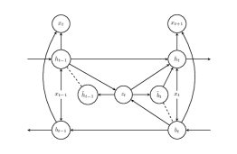
(a) Training phase of variational Bi-LSTM

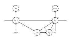
(b) Inference phase of variational Bi-LSTM

Figure 1: Graphical description of our proposed variational Bi-LSTM model during train phase (left) and inference phase (right). During training, each step $t$ is composed of an encoder which receives both the past and future summary via $\mathbf{h}_{t-1}$ and $\mathbf{b}_{t}$ respectively, and a decoder that generates $\tilde{\mathbf{h}}_{t-1}$ and $\tilde{\mathbf{b}}_{t}$ which are forced to be close enough to ${\mathbf{h}}_{t-1}$ and ${\mathbf{b}}_{t}$ using two auxiliary reconstruction costs (dashed lines). This dependence between backward and forward LSTM through the latent random variable encourages the forward LSTM to learn a richer representation. During inference, the backward LSTM is removed. In this case, $\mathbf{z}_{t}$ is sampled from the prior as in a typical VAE, which in our case, is defined as a function of $\mathbf{h}_{t-1}$.

2.1 Training and Inference

In the proposed variational Bi-LSTM, the latent variable $\mathbf{z}_{t}$ is inferred as

$$\mathbf{z}_{t}\sim q_{\phi}(\mathbf{z}_{t}|(\mathbf{h}_{t-1},\mathbf{b}_{t}))=\mathcal{N}(\boldsymbol{\mu}_{q,t},\textrm{diag}(\boldsymbol{\sigma}_{q,t}^{2})),$$ (6)

in which $[\boldsymbol{\mu}_{q,t},\boldsymbol{\sigma}^{2}_{q,t}]=f_{\phi}(\mathbf{h}_{t-1},\mathbf{b}_{t})$ where $f_{\phi}$ is a multi-layered feed-forward network with Gaussian outputs. We assume that the prior over $\mathbf{z}_{t}$ is a diagonal multivariate Gaussian distribution given by

$$p_{\theta}(\mathbf{z}_{t}|\mathbf{h}_{t-1})=\mathcal{N}(\boldsymbol{\mu}_{p,t},\textrm{diag}(\boldsymbol{\sigma}_{p,t}^{2})),\quad\textrm{where}\quad[\boldsymbol{\mu}_{p,t},\boldsymbol{\sigma}^{2}_{p,t}]=f_{\theta}(\mathbf{h}_{t-1}),$$ (7)

for a fully connected network $f_{\theta}$. This is important because, during generation (see Figure 1-right, for a graphical representation), we will not have access to the backward LSTM. In this case, as in a VAE, we will sample $\mathbf{z}_{t}$ from the prior during inference which only depends on the forward path. Since we define the prior to be a function of $\mathbf{h}_{t-1}$, the forward LSTM is encouraged during training to learn the dependence due to the backward hidden state $\mathbf{b}_{t}$.

The latent variable $\tilde{\mathbf{b}}_{t}$ is meant to model information coming from the future of the sequence. Its conditional distribution is given by

$$p_{\psi}(\tilde{\mathbf{b}}_{t}|\mathbf{z}_{t})=\mathcal{N}(\boldsymbol{\mu}_{\tilde{\mathbf{b}},t},\textrm{diag}(\boldsymbol{\sigma}_{\tilde{\mathbf{b}},t}^{2})),$$ (8)

where $[\boldsymbol{\mu}_{\tilde{\mathbf{b}},t},\boldsymbol{\sigma}^{2}_{\tilde{\mathbf{b}},t}]=f_{\psi}(\mathbf{z}_{t})$ for a fully connected neural network $f_{\psi}$ (See Figure 1(a)). To encourage the encoding of future information in $\tilde{\mathbf{b}}_{t}$, we maximize the probability of the true backward hidden state, $\mathbf{b}_{t}$, under the distribution $p_{\psi}$, as an auxiliary cost during training. In this way we treat $\tilde{\mathbf{b}}_{t}$ as a predictor of $\mathbf{b}_{t}$, similarly to what was done by Sordoni et al. (2017).

To capture information from the past in the latents, we similarly use $\tilde{\mathbf{h}}_{t-1}$ as a predictor of $\mathbf{h}_{t-1}$. This is accomplished by maximizing the probability of the latter under the conditional distribution of the former, $\log p_{\xi}(\tilde{\mathbf{h}}_{t-1}|\mathbf{z}_{t})$, as another auxiliary cost, where

$$p_{\xi}(\tilde{\mathbf{h}}_{t-1}|\mathbf{z}_{t})=\mathcal{N}(\boldsymbol{\mu}_{\tilde{\mathbf{h}},t},\textrm{diag}(\boldsymbol{\sigma}_{\tilde{\mathbf{h}},t}^{2})).$$ (9)

Here, $[\boldsymbol{\mu}_{\tilde{\mathbf{h}},t},\boldsymbol{\sigma}^{2}_{\tilde{\mathbf{h}},t}]$ is the output of a fully-connected neural network $f_{\xi}$ taking $\mathbf{z}_{t}$ as input. The auxiliary costs arising from distributions $p_{\xi}$ and $p_{\psi}$ teach the variational Bi-LSTM to encode past and future information into the latent space of $\mathbf{z}$.

We assume that the generating distribution $p_{\eta}(\mathbf{x}_{t+1}|\mathbf{x}_{1:t},\mathbf{z}_{1:t},\tilde{\mathbf{b}}_{t})$ is parameterized via a recurrent fully connected network, taking the form of either a Gaussian distribution output in the continuous case or categorical proportions output in the discrete (ie, one-hot) prediction case.

Finally, we define the Variational Bi-LSTM objective we use in this paper by instantiating the conditionals upon $\mathbf{x}_{1:t}$ used in Eq. 5 with functions $\mathbf{h}_{t}$ and $\mathbf{b}_{t}$ as,

$$\begin{split}\mathcal{L}(\mathbf{x};\boldsymbol{\Gamma},\boldsymbol{\xi})=\sum_{t=0}^{T}\underset{{\mathbf{z}_{t}\sim q_{\phi}(\mathbf{z}_{t}|\mathbf{h}_{t-1},\mathbf{b}_{t})}}{\mathbb{E}}\Big{[}&\ \underset{{\tilde{\mathbf{b}}_{t}\sim p_{\psi}(\tilde{\mathbf{b}}_{t}|\mathbf{z}_{t})}}{\mathbb{E}}\Big{[}\log p_{\eta}(\mathbf{x}_{t+1}|\mathbf{h}_{t})+\log p(\mathbf{x}_{t+1}|{\mathbf{b}}_{t})+\\ &\alpha\log p_{\psi}(\mathbf{b}_{t}|\mathbf{z}_{t})+\beta\log p_{\xi}(\mathbf{h}_{t-1}|\mathbf{z}_{t})\Big{]}\Big{]}-\\ &D_{KL}(q_{\phi}(\mathbf{z}_{t}|\mathbf{h}_{t-1},\mathbf{b}_{t})\|p_{\theta}(\mathbf{z}_{t}|\mathbf{h}_{t-1})),\\ \end{split}$$ (10)

where $\alpha$ and $\beta$ are non-negative real numbers denoting the coefficients of the auxiliary costs $\log p_{\psi}(\mathbf{b}_{t}|\mathbf{z}_{t})$ and $\log p_{\xi}(\mathbf{h}_{t-1}|\mathbf{z}_{t})$ respectively. These auxiliary costs ensure that $\tilde{\mathbf{h}}_{t}$ and $\tilde{\mathbf{b}}_{t}$ remain close to $\mathbf{h}_{t}$ and $\mathbf{b}_{t}$. All the parameters in $\boldsymbol{\Gamma}$ and $\boldsymbol{\xi}$ are updated based on backpropagation through time (Rumelhart et al., 1988) using the reparameterization trick (Kingma & Welling, 2014).

As a side note, we improve training convergence with a trick which we refer to as stochastic backprop, meant to ease learning of the latent variables. It is well known that autoregressive decoder models tend to ignore their stochastic variables (Bowman et al., 2015). Stochastic backprop is a technique to encourage that relevant summaries of the past and the future are encoded in the latent space. The idea is to stochastically skip gradients of the auxiliary costs with respect to the recurrent units from backpropagating through time. To achieve this, at each time step, a mask drawn from a Bernoulli distribution which governs whether to skip the gradient or to backpropagate it for a given data point.

3 Experimental results

In this section we demonstrate the effectiveness of our proposed model on several tasks. We present experimental results obtained when training Variational Bi-LSTM on various sequential datasets: Penn Treebank (PTB), IMDB, TIMIT, Blizzard, and Sequential MNIST. Our main goal is to ensure that the model proposed in Section 2 can benefit from a generated relevant summary of the future that yields competitive results. In all experiments, we train all the models using ADAM optimizer (Kingma & Ba, 2014) and we set all MLPs in Section 2 to have one hidden layer with leaky-ReLU hidden activation. All the models are implemented using Theano (Theano Development Team, 2016) and the code is available at https://anonymous.url.

Blizzard: Blizzard is a speech model dataset with 300 hours of English, spoken by a single female speaker. We report the average log-likelihood for half-second sequences (Fraccaro et al., 2016). In our experimental setting, we use 1024 hidden units for MLPs, 1024 LSTM units and 512 latents. Our model is trained using learning rate of 0.001 and minibatches of size 32 and we set $\alpha=\beta=1$. A fully factorized multivariate Gaussian distribution is used as the output distribution. The final lower bound estimation on TIMIT can be found in Table 1.

Table 1: The average of log-likelihood per sequence on Blizzard and TIMIT testset

Model	Blizzard	TIMIT
RNN-Gauss	3539	-1900
RNN-GMM	7413	26643
VRNN-I-Gauss	$\geq$ 8933	$\geq$ 28340
VRNN-Gauss	$\geq$ 9223	$\geq$ 28805
VRNN-GMM	$\geq$ 9392	$\geq$ 28982
SRNN (smooth+resq)	$\geq$ 11991	$\geq$ 60550
Z-Forcing  (Sordoni et al., 2017)	$\geq$ 14315	$\geq$ 68852
Variational Bi-LSTM	$\geq$ 17319	$\geq$ 73976

TIMIT: Another speech modeling dataset is TIMIT with 6300 English sentences read by 630 speakers. Like  Fraccaro et al. (2016), our model is trained on raw sequences of 200 dimensional frames. In our experiments, we use 1024 hidden units, 1024 LSTM units and 128 latent variables, and batch size of 128. We train the model using learning rate of 0.0001, $\alpha=0.001$ and $\beta=0$. The average log-likelihood for the sequences on test can be found in Table 1.

Sequential MNIST: We use the MNIST dataset which is binarized according to Murray & Salakhutdinov (2009) and we download it from Larochelle (2011). Our best model consists of 1024 hidden units, 1024 LSTM units and 256 latent variables. We train the model using a learning rate of 0.0001 and a batch size of 32. To reach the negative log-likelihood reported in Table 2, we set $\alpha=0.001$ and $\beta=0$.

Table 2: The average of negative log-likelihood on sequential MNIST

Models	Seq-MNIST
DBN 2hl (Germain et al., 2015)	$\approx$ 84.55
NADE (Uria et al., 2016)	88.33
EoNADE-5 2hl (Raiko et al., 2014)	84.68
DLGM 8  (Salimans et al., 2014)	$\approx$ 85.51
DARN 1hl (Gregor et al., 2015)	$\approx$ 84.13
BiHM (Bornschein et al., 2015)	$\approx$ 84.23
DRAW (Gregor et al., 2015)	$\leq$ 80.97
PixelVAE (Gulrajani et al., 2016)	$\approx$ 79.02▼
Prof. Forcing (Goyal et al., 2016)	79.58▼
PixelRNN${}_{\text{(1-layer)}}$ (Oord et al., 2016)	80.75
PixelRNN${}_{\text{(7-layer)}}$ (Oord et al., 2016)	79.20▼
Z-Forcing (Sordoni et al., 2017)	$\leq$ 80.09
Variational Bi-LSTM	$\leq$ 79.78

IMDB: It is a dataset consists of 350000 movie reviews (Diao et al., 2014) in which each sentence has less than 16 words and the vocabulary size is fixed to 16000 words. In this experiment, we use 500 hidden units, 500 LSTM units and latent variables of size 64. The model is trained with a batch size of 32 and a learning rate of 0.001 and we set $\alpha=\beta=1$. The word perplexity on valid and test dataset is shown in Table 3.

Table 3: Word perplexity on IMDB on valid and test sets

Model	Valid	Test
Gated Word-Char	70.60	70.87
Z-Forcing (Sordoni et al., 2017)	56.48	65.68
Variational Bi-LSTM	51.43	51.60

PTB: Penn Treebank (Marcus et al. (1993)) is a language model dataset consists of 1 million words. We train our model with 1024 LSTM units, 1024 hidden units, and the latent variables of size 128. We train the model using a standard Gaussian prior, a learning rate of 0.001 and batch size of 50 and we set $\alpha=\beta=1$. The model is trained to predict the next character in a sequence and the final bits per character on test and valid sets are shown in Table 4.

Table 4: Bits Per Character (BPC) on PTB valid and test sets

Model	Valid	Test
Unregularized LSTM	1.47	1.36
Weight noise	1.51	1.34
Norm stabilizer	1.46	1.35
Stochastic depth	1.43	1.34
Recurrent dropout	1.40	1.29
Zoneout (Krueger et al. (2016))	1.36	1.25
RBN (Cooijmans et al. (2016))	-	1.32
H-LSTM + LN (Ha et al. (2016))	1.28	1.25
3-HM-LSTM + LN (Chung et al., 2016)	-	1.24
2-H-LSTM + LN (Ha et al. (2016))	1.25	1.22
Z-Forcing	1.29	1.26
Variational Bi-LSTM	1.26	1.23

4 Ablation Studies

The goal of this section is to study the importance of the various components in our model and ensure that these components provide performance gains. The experiments are as follows:

Table 5: Perplexity on IMDB using different coefficient $\gamma$ for activity regularization

$\gamma$	0.001	1.	4.	8.	16.
Test perplexity	56.07	60.74	69.97	77.24	86.72

1. Reconstruction loss on $\mathbf{h}_{t}$ vs activity regularization on $\mathbf{h}_{t}$

Merity et al. (2017) study the importance of activity regularization (AR) on the hidden states of LSTMs given as,

$$\mathcal{R}_{AR} ={\gamma}\lVert\mathbf{h}_{t}\rVert_{2}^{2}.$$ (11)

Since our model’s reconstruction term on $\mathbf{h}_{t}$ can be decomposed as,

$$\lVert\mathbf{h}_{t}-\tilde{\mathbf{h}}_{t}\rVert_{2}^{2} =\lVert\mathbf{h}_{t}\rVert^{2}_{2}+\lVert\tilde{\mathbf{h}}_{t}\rVert^{2}_{2}-2\mathbf{h}_{t}^{T}\tilde{\mathbf{h}}_{t}$$ (12)

we perform experiments to confirm that the gains in our approach is not due to the $\ell^{2}$ regularization alone since our regularization encapsulates an $\ell^{2}$ term along with the dot product term.

To do so, we replace the auxiliary reconstruction terms in our objective with activity regularization using hyperparameter $\alpha\in\{0.001,1,4,8,16\}$ and study the test perplexity. The results are shown in table LABEL:table_ar_ablation. We find that in all the cases performance using activity regularization is worse compared with our best model shown in table 3.

Table 6: KL divergence of the Variational Bi-LSTM

Dataset	PTB	Seq-MNIST	IMDB	TIMIT	Blizzard
KL	0.001	0.02	0.18	3204.71	3799.79

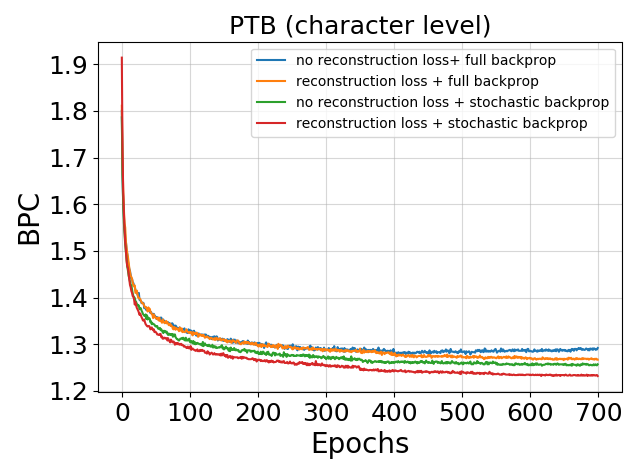
Figure 2: Evolution of validation set performance during training of Variational Bi-LSTMs with and without auxiliary reconstruction costs and stochastic backprop through auxiliary costs on PTB and Blizzard. We see that both the presence of reconstruction loss and stochastic back-propagation through them helps performance.

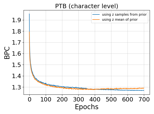
Figure 3: Evolution of bits per character (BPC) on PTB validation set with sampling latent variables $\mathbf{z}_{t}$ from $q_{\phi}(\mathbf{z}_{t}|\mathbf{h}_{t-1},\mathbf{b}_{t})$ during training vs. using the expected value of $\mathbf{z}_{t}$. Performance drops when $\mathbf{z}_{t}$ is not sampled. This shows sampling $\mathbf{z}_{t}$ randomly during training acts as a regularizer.

2. Use of parametric encoder prior vs. fixed Gaussian prior

In our variational Bi-LSTM model, we propose to have the encoder prior over $\mathbf{z}_{t}$ as a function of the previous forward LSTM hidden state $\mathbf{h}_{t-1}$. This is done to omit the need of the backward LSTM during inference because it is unavailable in practical scenarios since predictions are made in the forward direction. However, to study whether the model learns to use this encoder or not, we record the KL divergence value of the best validation model for the various datasets. The results are reported in table 6. We can see that the KL divergence values are large in the case of IMDB, TIMIT and Blizzard datasets, but small in the case of Seq-MNIST and PTB. To further explore, we run experiments on these datasets with fixed standard Gaussian prior like in the case of traditional VAE. Interestingly we find that the model with fixed prior performed similarly in the case of PTB, but hurt performance in the other cases, which can be explained given their large KL divergence values in the original experiments.

3. Effectiveness of auxiliary costs and stochastic back-propagation

In our model description, we propose to stochastically back propagate gradients through the auxiliary (reconstruction) costs, i.e., randomly choose to pass the gradients of the auxiliary cost or not. Here we evaluate the importance of the auxiliary costs and stochastic back-propagation. Figure 2 shows the evolution of validation performance on the Blizzard and PTB dataset. In both cases we see that both the auxiliary costs and stochastic back-propagation help the validation set performance.

4. Importance of sampling from VAE prior during training

We evaluate the effectiveness of sampling $\mathbf{z}_{t}$ from the prior during training vs. using the mean of the Gaussian prior. The validation set performance during training is shown in figure 3. It can be seen that sampling $\mathbf{z}_{t}$ leads to better generalization. Further, with the model trained with $\mathbf{z}_{t}$ sampled, we also evaluate if using samples is necessary during inference or not. Interestingly we find that during inference, the performance is identical in both cases; thus the deterministic mean of the prior can be used during inference.

5 Related Work

Variational auto-encoders (Kingma & Welling, 2014) can be easily combined with many deep learning models. They have been applied in the feed-forward setting but they have also found usage in RNNs to better capture variation in sequential data (Sordoni et al., 2017; Fraccaro et al., 2016; Chung et al., 2015; Bayer & Osendorfer, 2014). VAEs consists of several muti-layer neural networks as probabilistic encoders and decoders and training is based on the gradient on log-likelihood lower bound (as the likelihood is in general intractable) of the model parameters $\Gamma$ along with a reparametrization trick. The derived variational lower-bound $\mathcal{L}_{\Gamma}$ for an observed random variable $\mathbf{x}$ is:

$$\log p(\mathbf{x})\geq\mathcal{L}_{\Gamma}=\underset{\mathbf{z}\sim q_{\phi}(\mathbf{z}|\mathbf{x})}{\mathbb{E}}\left[\log\frac{p(\mathbf{x},\mathbf{z})}{q_{\phi}(\mathbf{z}|\mathbf{x})}\right]=\underset{\mathbf{z}\sim q_{\phi}(\mathbf{z}|\mathbf{x})}{\mathbb{E}}\Big{[}\ln p_{\theta}(\mathbf{x}|\mathbf{z})\Big{]}-D_{KL}(q_{\phi}(\mathbf{z}|\mathbf{x})\|p_{\theta}(\mathbf{z})),$$ (13)

where $D_{KL}$ denotes the Kullback-Leibler divergence and $p_{\theta}$ is the prior over a latent variable $\mathbf{z}$. The KL divergence term can be expressed as the difference between the cross-entropy of the prior w.r.t. $q_{\phi}(\mathbf{z}|\mathbf{x})$ and the entropy of $q_{\phi}(\mathbf{z}|\mathbf{x})$, and fortunately, it can be analytically computed and differentiated for some distribution families like Gaussians. Although maximizing the log-likelihood corresponds to minimizing the KL divergence, we have to ensure that the resulting $q_{\phi}$ remains far enough from an undesired equilibrium state where $q_{\phi}(\mathbf{z}|\mathbf{x})$ is almost everywhere equal to the prior over latent variables. Combining recurrent neural networks with variational auto encoders can lead to powerful generative models that are capable of capturing the variations in data, however, they suffer badly from this optimization issue as discussed by Bowman et al. (2015).

However, VAEs have successfully been applied to Bi-LSTMs by Sordoni et al. (2017) through a technique called Z-forcing. It is a powerful generative auto-regressive model which is trained using the following variational evidence lower-bound

$$\begin{split}\mathcal{L}(\mathbf{x};\theta,\phi,\xi)=\sum_{t}\underset{q_{\phi}(\mathbf{z}_{t}|\mathbf{x})}{\mathbb{E}}&\Big{[}\log p_{\theta}(\mathbf{x}_{t+1}|\mathbf{x}_{1:t},\mathbf{z}_{1:t})\Big{]}-D_{KL}(q_{\phi}(\mathbf{z}_{t}|\mathbf{x})\|p_{\theta}(\mathbf{z}_{t}|\mathbf{x}_{1:t-1},\mathbf{z}_{1:t-1}))\end{split}$$

plus an auxiliary cost as a regularizer which is defined as $\log p_{\xi}(\mathbf{b}_{t}|\mathbf{z}_{t})$. It is shown that the auxiliary cost helps in improving the final performance; however during inference the backward reconstructions are not used in their approach. In our ablation study section below, we show experimentally that this connection is important for improving the performance of Bi-LSTMs as is the case in our model.

Twin networks on the other hand is a deterministic method which enforces the hidden states of the forward and backward paths of a Bi-LSTM to be similar. Specifically, this is done by adding as a regularization $\ell^{2}$ norm of difference between the pair of hidden states at each time step. The intuition behind this regularization is to encourage the hidden representations to be compatible towards future predictions. Notice a difference between twin networks and our approach is that twin networks forces the hidden states of both the LSTMs to be similar to each other while our approach directly feeds a latent variable $\tilde{\mathbf{b}}_{t}$ to the forward LSTM that is trained to be similar to the backward LSTM hidden state ${\mathbf{b}}_{t}$. Hence while twin networks discard information from the backward path during inference, our model encourages the use of this information.

6 Conclusion

We propose Variational Bi-LSTM as an auto-regressive generative model by framing a joint objective that effectively creates a channel for exchanging information between the forward and backward LSTM. We achieve this by deriving a variational lower bound of the joint likelihood of the temporal data sequence. We empirically show that our variational Bi-LSTM model acts as a regularizer for the forward LSTM and leads to performance improvement on different benchmark sequence generation problems. We also show through ablation studies the importance of the various components in our model.

Appendix

A: Derivation of variation lower bound ${\mathcal{L}}_{\boldsymbol{\Gamma}}$ in equation (5) in more details:

$$\begin{split}\log p(\mathbf{x};\boldsymbol{\Gamma})&=\log\Big{[}\prod_{t=0}^{T}\int_{\mathbf{z}_{t}}\int_{\tilde{\mathbf{b}}_{t}}\Big{[}p_{\eta}(\mathbf{x}_{t+1}|\mathbf{x}_{1:t},\mathbf{z}_{t},\tilde{\mathbf{b}}_{t})p_{\psi}(\tilde{\mathbf{b}}_{t}|\mathbf{z}_{t})p_{\theta}(\mathbf{z}_{t}|\mathbf{x}_{1:t})\Big{]}d\tilde{\mathbf{b}}_{t}d\mathbf{z}_{t}\Big{]}\\ &=\sum_{t=0}^{T}\log\Big{[}\int_{\mathbf{z}_{t}}p_{\theta}(\mathbf{z}_{t}|\mathbf{x}_{1:t})\int_{\tilde{\mathbf{b}}_{t}}\Big{[}p_{\eta}(\mathbf{x}_{t+1}|\mathbf{x}_{1:t},\mathbf{z}_{t},\tilde{\mathbf{b}}_{t})p_{\psi}(\tilde{\mathbf{b}}_{t}|\mathbf{z}_{t})\Big{]}d\tilde{\mathbf{b}}_{t}d\mathbf{z}_{t}\Big{]}\\ &=\sum_{t=0}^{T}\log\Big{[}\int_{\mathbf{z}_{t}}q_{\phi}(\mathbf{z}_{t}|\mathbf{x}_{1:t})\frac{p_{\theta}(\mathbf{z}_{t}|\mathbf{x}_{1:t})}{q_{\phi}(\mathbf{z}_{t}|\mathbf{x}_{1:t})}\int_{\tilde{\mathbf{b}}_{t}}\Big{[}p_{\eta}(\mathbf{x}_{t+1}|\mathbf{x}_{1:t},\mathbf{z}_{t},\tilde{\mathbf{b}}_{t})p_{\psi}(\tilde{\mathbf{b}}_{t}|\mathbf{z}_{t})\Big{]}d\tilde{\mathbf{b}}_{t}d\mathbf{z}_{t}\Big{]}\\ &\geq\sum_{t=0}^{T}\int_{\mathbf{z}_{t}}q_{\phi}(\mathbf{z}_{t}|\mathbf{x}_{1:t})\log\Big{[}\frac{p_{\theta}(\mathbf{z}_{t}|\mathbf{x}_{1:t})}{q_{\phi}(\mathbf{z}_{t}|\mathbf{x}_{1:t})}\int_{\tilde{\mathbf{b}}_{t}}\Big{[}p_{\eta}(\mathbf{x}_{t+1}|\mathbf{x}_{1:t},\mathbf{z}_{t},\tilde{\mathbf{b}}_{t})p_{\psi}(\tilde{\mathbf{b}}_{t}|\mathbf{z}_{t})\Big{]}d\tilde{\mathbf{b}}_{t}d\mathbf{z}_{t}\Big{]}\\ &=\sum_{t=0}^{T}\int_{\mathbf{z}_{t}}\Big{[}q_{\phi}(\mathbf{z}_{t}|\mathbf{x}_{1:t})\log(\frac{p_{\theta}(\mathbf{z}_{t}|\mathbf{x}_{1:t})}{q_{\phi}(\mathbf{z}_{t}|\mathbf{x}_{1:t})})\\ &\quad\quad+q_{\phi}(\mathbf{z}_{t}|\mathbf{x}_{1:t})\log\Big{[}\int_{\tilde{\mathbf{b}}_{t}}\Big{[}p_{\eta}(\mathbf{x}_{t+1}|\mathbf{x}_{1:t},\mathbf{z}_{t},\tilde{\mathbf{b}}_{t})p_{\psi}(\tilde{\mathbf{b}}_{t}|\mathbf{z}_{t})\Big{]}d\tilde{\mathbf{b}}_{t}d\mathbf{z}_{t}\Big{]}\\ &=\sum_{t=0}^{T}\Big{[}\int_{\mathbf{z}_{t}}q_{\phi}(\mathbf{z}_{t}|\mathbf{x}_{1:t})\log\Big{[}\int_{\tilde{\mathbf{b}}_{t}}\Big{[}p_{\eta}(\mathbf{x}_{t+1}|\mathbf{x}_{1:t},\mathbf{z}_{t},\tilde{\mathbf{b}}_{t})p_{\psi}(\tilde{\mathbf{b}}_{t}|\mathbf{z}_{t})\Big{]}d\tilde{\mathbf{b}}_{t}d\mathbf{z}_{t}\Big{]}\\ &\quad\quad-D_{KL}(q_{\phi}(\mathbf{z}_{t}|\mathbf{x}_{1:t})\|p_{\theta}(\mathbf{z}_{t}|\mathbf{x}_{1:t}))\Big{]}\\ &\geq\sum_{t=0}^{T}\Big{[}\int_{\mathbf{z}_{t}}q_{\phi}(\mathbf{z}_{t}|\mathbf{x}_{1:t})\int_{\tilde{\mathbf{b}}_{t}}p_{\psi}(\tilde{\mathbf{b}}_{t}|\mathbf{z}_{t})\log\Big{[}p_{\eta}(\mathbf{x}_{t+1}|\mathbf{x}_{1:t},\mathbf{z}_{t},\tilde{\mathbf{b}}_{t})\Big{]}d\tilde{\mathbf{b}}_{t}d\mathbf{z}_{t}\\ &\quad\quad-D_{KL}(q_{\phi}(\mathbf{z}_{t}|\mathbf{x}_{1:t})\|p_{\theta}(\mathbf{z}_{t}|\mathbf{x}_{1:t}))\Big{]}\\ &\approx\sum_{t=0}^{T}\underset{{\mathbf{z}_{t}\sim q_{\phi}(\mathbf{z}_{t}|\mathbf{x}_{1:t})}}{\mathbb{E}}\underset{{\tilde{\mathbf{b}}_{t}\sim p_{\psi}(\tilde{\mathbf{b}}_{t}|\mathbf{z}_{t})}}{\mathbb{E}}\Big{[}\log p_{\eta}(\mathbf{x}_{t+1}|\mathbf{x}_{1:t},\mathbf{z}_{t},\tilde{\mathbf{b}}_{t})\Big{]}-D_{KL}(q_{\phi}(\mathbf{z}_{t}|\mathbf{x}_{1:t})\|p_{\theta}(\mathbf{z}_{t}|\mathbf{x}_{1:t})).\end{split}$$

References

- Arik et al. (2017) Sercan O Arik, Mike Chrzanowski, Adam Coates, Gregory Diamos, Andrew Gibiansky, Yongguo Kang, Xian Li, John Miller, Jonathan Raiman, Shubho Sengupta, et al. Deep voice: Real-time neural text-to-speech. arXiv preprint arXiv:1702.07825, 2017.
- Bayer & Osendorfer (2014) Justin Bayer and Christian Osendorfer. Learning stochastic recurrent networks. arXiv preprint arXiv:1411.7610, 2014.
- Bornschein et al. (2015) Jörg Bornschein, Samira Shabanian, Asja Fischer, and Yoshua Bengio. Training opposing directed models using geometric mean matching. CoRR, abs/1506.03877, 2015. URL http://arxiv.org/abs/1506.03877.
- Bowman et al. (2015) Samuel R Bowman, Luke Vilnis, Oriol Vinyals, Andrew M Dai, Rafal Jozefowicz, and Samy Bengio. Generating sentences from a continuous space. arXiv preprint arXiv:1511.06349, 2015.
- Chung et al. (2014) Junyoung Chung, Caglar Gulcehre, KyungHyun Cho, and Yoshua Bengio. Empirical evaluation of gated recurrent neural networks on sequence modeling. arXiv preprint arXiv:1412.3555, 2014.
- Chung et al. (2015) Junyoung Chung, Kyle Kastner, Laurent Dinh, Kratarth Goel, Aaron C Courville, and Yoshua Bengio. A recurrent latent variable model for sequential data. In Advances in neural information processing systems, pp. 2980–2988, 2015.
- Cooijmans et al. (2016) Tim Cooijmans, Nicolas Ballas, César Laurent, and Aaron C. Courville. Recurrent batch normalization. CoRR, abs/1603.09025, 2016. URL http://arxiv.org/abs/1603.09025.
- Diao et al. (2014) Qiming Diao, Minghui Qiu, Chao-Yuan Wu, Alexander J Smola, Jing Jiang, and Chong Wang. Jointly modeling aspects, ratings and sentiments for movie recommendation (jmars). In Proceedings of the 20th ACM SIGKDD international conference on Knowledge discovery and data mining, pp. 193–202, 2014.
- Fraccaro et al. (2016) Marco Fraccaro, Søren Kaae Sønderby, Ulrich Paquet, and Ole Winther. Sequential neural models with stochastic layers. In Advances in Neural Information Processing Systems, pp. 2199–2207, 2016.
- Gal & Ghahramani (2016) Yarin Gal and Zoubin Ghahramani. A theoretically grounded application of dropout in recurrent neural networks. In Advances in neural information processing systems, pp. 1019–1027, 2016.
- Germain et al. (2015) Mathieu Germain, Karol Gregor, Iain Murray, and Hugo Larochelle. Made: Masked autoencoder for distribution estimation. In ICML, pp. 881–889, 2015.
- Goyal et al. (2016) Anirudh Goyal, Alex Lamb, Ying Zhang, Saizheng Zhang, Aaron C. Courville, and Yoshua Bengio. Professor forcing: A new algorithm for training recurrent networks. In Advances in Neural Information Processing Systems 29: Annual Conference on Neural Information Processing Systems 2016, December 5-10, 2016, Barcelona, Spain, pp. 4601–4609, 2016. URL http://papers.nips.cc/paper/6099-professor-forcing-a-new-algorithm-for-training-recurrent-networks.
- Gregor et al. (2015) Karol Gregor, Ivo Danihelka, Alex Graves, Danilo Jimenez Rezende, and Daan Wierstra. Draw: A recurrent neural network for image generation. arXiv preprint arXiv:1502.04623, 2015.
- Gulrajani et al. (2016) Ishaan Gulrajani, Kundan Kumar, Faruk Ahmed, Adrien Ali Taiga, Francesco Visin, David Vazquez, and Aaron Courville. Pixelvae: A latent variable model for natural images. arXiv preprint arXiv:1611.05013, 2016.
- Ha et al. (2016) David Ha, Andrew M. Dai, and Quoc V. Le. Hypernetworks. CoRR, abs/1609.09106, 2016. URL http://arxiv.org/abs/1609.09106.
- Hochreiter & Schmidhuber (1997) Sepp Hochreiter and Jürgen Schmidhuber. Long short-term memory. Neural computation, 9(8):1735–1780, 1997.
- Kingma & Ba (2014) Diederik Kingma and Jimmy Ba. Adam: A method for stochastic optimization. arXiv preprint arXiv:1412.6980, 2014.
- Kingma & Welling (2014) Diederik P Kingma and Max Welling. Stochastic Gradient VB and the Variational Auto-Encoder. 2nd International Conference on Learning Representationsm (ICLR), pp. 1–14, 2014. ISSN 0004-6361. doi: 10.1051/0004-6361/201527329. URL http://arxiv.org/abs/1312.6114.
- Krueger et al. (2016) David Krueger, Tegan Maharaj, János Kramár, Mohammad Pezeshki, Nicolas Ballas, Nan Rosemary Ke, Anirudh Goyal, Yoshua Bengio, Hugo Larochelle, Aaron C. Courville, and Chris Pal. Zoneout: Regularizing rnns by randomly preserving hidden activations. CoRR, abs/1606.01305, 2016. URL http://arxiv.org/abs/1606.01305.
- Larochelle (2011) Hugo Larochelle. Binarized mnist dataset. 2011. URL http://www.cs.toronto.edu/~larocheh/public/datasets/binarized_mnist/binarized_mnist_train.amat.
- Marcus et al. (1993) Mitchell P. Marcus, Mary Ann Marcinkiewicz, and Beatrice Santorini. Building a large annotated corpus of english: The penn treebank. Comput. Linguist., 19(2):313–330, June 1993. ISSN 0891-2017. URL http://dl.acm.org/citation.cfm?id=972470.972475.
- Mehri et al. (2016) Soroush Mehri, Kundan Kumar, Ishaan Gulrajani, Rithesh Kumar, Shubham Jain, Jose Sotelo, Aaron Courville, and Yoshua Bengio. Samplernn: An unconditional end-to-end neural audio generation model. arXiv preprint arXiv:1612.07837, 2016.
- Merity et al. (2017) Stephen Merity, Bryan McCann, and Richard Socher. Revisiting activation regularization for language rnns. arXiv preprint arXiv:1708.01009, 2017.
- Murray & Salakhutdinov (2009) Iain Murray and Ruslan R Salakhutdinov. Evaluating probabilities under high-dimensional latent variable models. In D. Koller, D. Schuurmans, Y. Bengio, and L. Bottou (eds.), Advances in Neural Information Processing Systems 21, pp. 1137–1144. Curran Associates, Inc., 2009. URL http://papers.nips.cc/paper/3584-evaluating-probabilities-under-high-dimensional-latent-variable-models.pdf.
- Oord et al. (2016) Aaron van den Oord, Nal Kalchbrenner, and Koray Kavukcuoglu. Pixel recurrent neural networks. arXiv preprint arXiv:1601.06759, 2016.
- Pascanu et al. (2012) Razvan Pascanu, Tomas Mikolov, and Yoshua Bengio. Understanding the exploding gradient problem. CoRR, abs/1211.5063, 2012. URL http://arxiv.org/abs/1211.5063.
- Raiko et al. (2014) Tapani Raiko, Yao Li, Kyunghyun Cho, and Yoshua Bengio. Iterative neural autoregressive distribution estimator nade-k. In Advances in neural information processing systems, pp. 325–333, 2014.
- Rumelhart et al. (1988) David E Rumelhart, Geoffrey E Hinton, and Ronald J Williams. Learning representations by back-propagating errors. Cognitive modeling, 5(3):1, 1988.
- Salimans et al. (2014) Tim Salimans, Diederik P Kingma, and Max Welling. Markov chain monte carlo and variational inference: Bridging the gap. arXiv preprint arXiv:1410.6460, 2014.
- Serdyuk et al. (2017) Dmitriy Serdyuk, Rosemary Nan Ke, Alessandro Sordoni, Chris Pal, and Yoshua Bengio. Twin networks: Using the future as a regularizer. arXiv preprint arXiv:1708.06742, 2017.
- Sordoni et al. (2017) Alessandro Sordoni, Anirudh Goyal ALIAS PARTH GOYAL, Marc-Alexandre Cote, Nan Ke, and Yoshua Bengio. Z-forcing: Training stochastic recurrent networks. In Advances in Neural Information Processing Systems. 2017. URL https://nips.cc/Conferences/2017/Schedule?showEvent=9439.
- Sotelo et al. (2017) Jose Sotelo, Soroush Mehri, Kundan Kumar, Joao Felipe Santos, Kyle Kastner, Aaron Courville, and Yoshua Bengio. Char2wav: End-to-end speech synthesis. 2017.
- Srivastava et al. (2014) Nitish Srivastava, Geoffrey E Hinton, Alex Krizhevsky, Ilya Sutskever, and Ruslan Salakhutdinov. Dropout: a simple way to prevent neural networks from overfitting. Journal of machine learning research, 15(1):1929–1958, 2014.
- Theano Development Team (2016) Theano Development Team. Theano: A Python framework for fast computation of mathematical expressions. arXiv e-prints, abs/1605.02688, May 2016. URL http://arxiv.org/abs/1605.02688.
- Uria et al. (2016) Benigno Uria, Marc-Alexandre Côté, Karol Gregor, Iain Murray, and Hugo Larochelle. Neural autoregressive distribution estimation. Journal of Machine Learning Research, 17(205):1–37, 2016.
- Wang et al. (2017) Yuxuan Wang, RJ Skerry-Ryan, Daisy Stanton, Yonghui Wu, Ron J Weiss, Navdeep Jaitly, Zongheng Yang, Ying Xiao, Zhifeng Chen, Samy Bengio, et al. Tacotron: Towards end-to-end speech syn. arXiv preprint arXiv:1703.10135, 2017.
- Zaremba et al. (2014) Wojciech Zaremba, Ilya Sutskever, and Oriol Vinyals. Recurrent neural network regularization. arXiv preprint arXiv:1409.2329, 2014.