Supplementary material: The interplay of activity and filament flexibility determines the emergent properties of active nematics

S1 Simulation movies

Animations of simulation trajectories (showing $1/16$ of the simulation box) are provided for the following parameter sets, with $k_{\text{b}}=300$ and $\tau_{1}=0.2$ in all cases:

• fa5_k500_t0p2.mp4:  $\kappa_{\text{eff}}=20:\kappa=500,{f^{\text{a}}}=5$

• fa5_k2500_t0p2.mp4:  $\kappa_{\text{eff}}=100:\kappa=2500,{f^{\text{a}}}=5$

• fa10_k200_t0p2.mp4:  $\kappa_{\text{eff}}=2:\kappa=200,{f^{\text{a}}}=10$

• fa10_k2500_t0p2.mp4:  $\kappa_{\text{eff}}=25:\kappa=2500,{f^{\text{a}}}=10$

• fa30_k10000_t0p2.mp4:  $\kappa_{\text{eff}}=11:\kappa=10^{4},{f^{\text{a}}}=30$

In the videos, white arrows indicate positions and orientations of $+\frac{1}{2}$ defects and white dots indicate positions of $-\frac{1}{2}$ defects. Filament beads are colored according to the orientations of the local tangent vector.

S2 Model and simulation details

Interaction potentials: We simulate the dynamics for the system of active filaments according to the following Langevin equation for each filament $\alpha$ and bead $i$ (with filaments indexed by Greek letters, $\alpha=1\ldots N$, and beads within a filament indexed in Roman, $i=1\ldots M$)

$$m\ddot{\mathbf{r}}_{\alpha,i}=\mathbf{f}^{\text{a}}_{\alpha,i}-\gamma\dot{\mathbf{r}}_{\alpha,i}-\nabla_{\mathbf{r}_{\alpha,i}}U+\mathbf{R}_{\alpha,i}(t).$$ (S1)

with $m$ as the bead mass, $\mathbf{r}_{\alpha,i}$ as the bead position, ${f^{\text{a}}}$ as the active force, $U$ as the interaction potential which gives rise to the conservative forces, $\gamma$ as the friction coefficient providing the damping and $\mathbf{R}_{\alpha,i}(t)$ as a delta-correlated thermal noise with zero mean and variance $\langle\mathbf{R}_{\alpha,i}(t)\cdot\mathbf{R}_{\beta,j}(t^{\prime})\rangle=4\gamma k_{\text{B}}T\delta_{\alpha,\beta}\delta_{ij}\delta(t-t^{\prime})$.

The interaction potential includes three contributions which respectively account for non-bonded interactions between all bead pairs, stretching of each bond, and the angle potential between each pair of neighboring bonds:

$$U(\{\mathbf{r}_{\alpha,i}\})= \frac{1}{2}\sum_{\alpha,\beta=1}^{N}\sum_{i,j=1}^{M}\left(1-\delta_{\alpha,\beta}\delta_{i,j}\right)U_{\text{nb}}(\left|\mathbf{r}_{\beta,j}-\mathbf{r}_{\alpha,i}\right|)$$

$$+ \sum_{\alpha=1}^{N}\sum_{i=2}^{M}U_{\text{s}}(\left|\mathbf{r}_{\alpha,i}-\mathbf{r}_{\alpha,i-1}\right|)$$

$$+ \sum_{\alpha=1}^{N}\sum_{i=3}^{M}U_{\text{angle}}(\theta_{\alpha,i,i-1,i-2})$$ (S2)

with $\theta_{\alpha,i,j,k}$ the angle made by the bead triplet $\{i,j,k\}$ on filament $\alpha$. The non-bonded interactions account for steric repulsion and are modeled with the Weeks-Chandler-Anderson potentialWeeks et al. (1971)

$$U_{\text{nb}}(r)=4\varepsilon\left((\sigma/r)^{12}-(\sigma/r)^{6}+1/4\right)\Theta(2^{1/6}\sigma-r)$$ (S3)

with $\varepsilon$ controlling the strength of steric repulsion and $\Theta(x)$ the Heaviside function specifying the cutoff. Bond stretching is controlled by a FENE potential Kremer and Grest (1990)

$$U_{\text{s}}(r)=-1/2k_{\text{b}}R_{0}^{2}\ln\left(1-\left({r}/{R_{0}}\right)^{2}\right)$$ (S4)

with bond strength $k_{\text{b}}$ and maximum bond length $R_{0}$. The angle potential is given by

$$U_{\text{angle}}(\theta)=\kappa\left(\theta-\pi\right)^{2}$$ (S5)

where $\kappa$ is the filament bending modulus.

Finally, activity is modeled as a propulsive force on every bead directed along the filament tangent toward its head. To render the activity nematic, the head and tail of each filament are switched at stochastic intervals so that the force direction on each bead rotates by $180$ degrees. In particular, the active force has the form, $\mathbf{f}^{\text{a}}_{\alpha,i}(t)=\eta_{\alpha}(t){f^{\text{a}}}\mathbf{t}_{\alpha,i}$, where ${f^{\text{a}}}$ parameterizes the activity strength, and $\eta_{\alpha}(t)$ is a stochastic variable associated with filament $\alpha$ that changes its values between 1 and $-1$ on Poisson distributed intervals with mean $\tau_{1}$, so that $\tau_{1}$ controls the reversal frequency. The local tangent vector $\mathbf{t}_{\alpha,i}$ along the filament contour at a bead $i$ is calculated as

$$\mathbf{t}_{\alpha,i}=\begin{cases}\frac{\mathbf{r}_{\alpha,i+1}-\mathbf{r}_{\alpha,i-1}}{|\mathbf{r}_{\alpha,i+1}-\mathbf{r}_{\alpha,i-1}|},&\text{for }i=2,...,M-1\\ \frac{\mathbf{r}_{\alpha,2}-\mathbf{r}_{\alpha,1}}{|\mathbf{r}_{\alpha,2}-\mathbf{r}_{\alpha,1}|},&\text{for }i=1\\ \frac{\mathbf{r}_{\alpha,M}-\mathbf{r}_{\alpha,M-1}}{|\mathbf{r}_{\alpha,M}-\mathbf{r}_{\alpha,M-1}|}&\text{for }i=M.\end{cases}$$

Simulations and parameter values: We set mass of the each bead to $m=1$ and the damping coefficient to $\gamma=2$. With these parameters inertia is non-negligible. In the future, we plan to systematically investigate the effect of damping. We report lengths and energies in units of the bead diameter $\sigma=1$ and the thermal energy at a reference state, $k_{\text{B}}T_{\text{ref}}$. Time is measured in units of $\tau=\sqrt{m\sigma^{2}/k_{\text{B}}T_{\text{ref}}}$. Eqs. (S1) were integrated with time step $\delta t=10^{-3}\tau$ using LAMMPS Plimpton (1995), with an in-house modification to include the active propulsion force. We set the repulsion parameter $\varepsilon=k_{\text{B}}T_{\text{ref}}$ (the results are insensitive to the value of $\varepsilon$ provided it is sufficiently high to avoid filament overlap). We performed simulations in a $A=840\times 840\sigma^{2}$ periodic simulation box, with $N=19404$ filaments each with $M=20$ beads, so that the packing fraction $\phi=MN\sigma^{2}/A\approx 0.55$.

In the FENE bond potential, $R_{0}$ is set to $1.5\sigma$ and $k_{\text{b}}=300k_{\text{B}}T_{\text{ref}}/\sigma^{2}$ for the simulations in the main text (see next paragraph). The temperature is set to $T=3.0k_{\text{B}}T_{\text{ref}}$. These parameters lead to a mean bond length of $b\approx 0.84\sigma$, which ensures that filaments are non-penetrable for the parameter space explored in this work. Finally, $L=(M-1)b$ is the mean filament length. In semiflexible limit, the stiffness $\kappa$ in the discrete model is related to the continuum bending modulus $\tilde{\kappa}$ as $\kappa\approx\tilde{\kappa}/2b$, and thus the persistence length is given by $l_{\text{p}}=2b\kappa/k_{\text{B}}T$.

We performed two sets of simulations. Initially, we set the FENE bond strength $k_{\text{b}}=30k_{\text{B}}T_{\text{ref}}/\sigma^{2}$ and $\tau_{1}=\tau$, thus maintaining the reversal frequency of active propulsion to a fixed value while varying filament stiffness, $\kappa\in[100,2500]k_{\text{B}}T_{\text{ref}}$ and the magnitude of the active force. However, for these parameters we discovered that interpenetration of filaments becomes possible at large propulsion velocities, thus limiting the simulations to ${f^{\text{a}}}\leq 10$. To enable investigating higher activity values, we therefore performed a second set of simulations (those reported in the main text) with higher FENE bond strength, $k_{\text{b}}=300k_{\text{B}}T_{\text{ref}}/\sigma^{2}$ and shorter reversal timescale $\tau_{1}=0.2$, with $\kappa\in[100,10000]k_{\text{B}}T_{\text{ref}}$. This enables simulating activity values up to ${f^{\text{a}}}\leq 30$.

The shorter reversal timescale was needed in the new set of simulations because when the product ${f^{\text{a}}}\tau$ exceeds a characteristic collision length scale the self-propulsion becomes polar in nature and model is no longer a good description of an active nematic. In particular, the filaments behave as polar self-propelled rods, as evidenced by the formation of polar clusters Peruani et al. (2006); McCandlish et al. (2012); Weitz et al. (2015); Ginelli et al. (2010); Peruani et al. (2012). Interestingly, increasing $k_{\text{b}}$ increases the rate of defect formation and decreases the threshold value of ${f^{\text{a}}}\tau$ above which phase separation occurs. We monitored the existence of phase separation by measuring local densities within simulation boxes (see below). We found no significant phase separation (except on short scales, see below) or formation of polar clusters for any of the simulations described here, indicating the systems were in the nematic regime. Within the nematic regime, increasing $k_{\text{b}}$ does not qualitatively change results or scaling relations, although it does quantitatively shift properties such as the defect density. The scaling of defect density with $\kappa$ and ${f^{\text{a}}}$ for the simulations with $k_{\text{b}}=30$ is shown in Fig. S1.

In our simulations we have fixed the filament length at $M=20$ beads. Exploratory simulations showed that varying $M$ does not change the scaling of observables with $\kappa_{\text{eff}}$, although it shifts properties such as the defect density since the total active force per filament goes as ${f^{\text{a}}}M$. The maximum persistence length above which scaling laws fail is also proportional to filament length: $\kappa_{\text{eff}}^{\text{max}}=k_{\text{B}}TM/2b$

Initialization: We initialized the system by first placing the filaments in completely extended configurations (all bonds parallel and all bond lengths set to $b$), on a rectangular lattice aligned with the simulation box, with filaments oriented along one of the lattice vectors. We then allowed this initial configuration to relax by simulating for $10^{4}\tau$, before performing production runs of $\sim 4\times 10^{4}\tau$. As noted in the main text, the equilibration time of $10^{4}\tau$ was chosen based on the fact that in all simulated systems the defect density had reached steady state by this time. We also confirmed that other observables of interest have reached steady state at this time. In the limit of high stiffness or low activity, we found that defect nucleation from the unphysically crystalline initial condition did not occur on computationally accessible timescales, thus prohibiting relaxation. In these cases, we used an alternative initial configuration, with filaments arranged into four rectangular lattices, each placed in one quadrant of the simulation box such that adjacent (non-diagonal) lattices are orthogonal.

Analysis: To analyze our simulation trajectories within the framework of liquid crystal theory, we calculated the local nematic tensor as $Q_{\alpha\beta}(r_{ij})=\sum_{k,|r_{k}-r_{ij}|<5\sigma}(\hat{t}_{k\alpha}\hat{t}_{k\beta}-\frac{1}{2}{\delta_{\alpha\beta}})$ and the density field $\rho$ on a $1000\times 1000$ grid, where, $r_{ij}$ is the position of the grid point and $r_{k}$ and $t_{k}$ are the positions and tangent vectors of all segments. We then evaluated the local nematic order parameter, $S$ and director $\hat{n}$ as the largest eigenvalue of $Q$ and corresponding eigenvector. We identified defects in the director field and their topological charges using the procedure described in section S9 below. To compare the magnitudes of splay and bend deformations in our active systems to those that occur at equilibrium, we calculated elastic constants of our system at equilibrium (${f^{\text{a}}}=0$) using the free energy perturbation technique proposed by Joshi et al. Joshi et al. (2014). We performed these equilibrium calculations on a box of size $64\times 64\sigma^{2}$.

S3 Additional figures on scaling of active nematic characteristics with $\kappa_{\text{eff}}$

We present data on defect density from the alternative data set described in section S2 in Fig. S1, and an explicit listing of parameter values for Fig. 3 in the main text in Fig. S2.

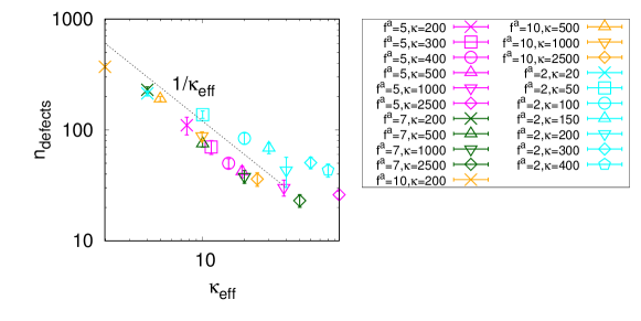
Figure S1: Number of defects as a function of $\kappa_{\text{eff}}$ for the alternative dataset, with FENE bond strength $k_{\text{b}}=30$ and active reversal period, $\tau_{1}=1$. Notice that we observe data collapse for all parameters with ${f^{\text{a}}}\geq 5$, but not for the lowest activity ${f^{\text{a}}}=2$ (light blue symbols), when the system begins to lose nematic order (see Fig. S7c below) and the active force strength becomes comparable to thermal forces.

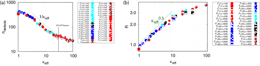
Figure S2: Specification of all data points considered for the main data set ($k_{\text{b}}=300$ and $\tau_{1}=0.2$) (a) Defect density as a function of $\kappa_{\text{eff}}$ for indicated values of ${f^{\text{a}}}$ and $\kappa$. (b) Ratio of splay/bend ($R$, defined in the main text) as a function of $\kappa_{\text{eff}}$ for indicated values of ${f^{\text{a}}}$ and $\kappa$.

S4 Estimating the individual filament persistence length

In this section we describe estimates of the effective persistence length measured from the tangent fluctuations of individual filaments. We performed these measurements both on individual filaments within a bulk active nematic, and isolated individual filaments to distinguish single-chain and multi-chain effects on the effective persistence length.

In a continuum limit, the total bending energy of a semiflexible filament it is well approximated by the wormlike chain model Doi and Edwards (1988),

$$H_{\text{bend}}=\frac{\tilde{\kappa}}{2}\int_{0}^{L}\left(\frac{d\theta}{ds}\right)^{2}ds$$ (S6)

where the integration is over the filament contour length, $L$, parameterized by $s$, $\tilde{\kappa}$ is the continuum bending modulus, and $\theta(s)$ is the tangent angle along the contour.

For a normal-mode analysis of the bending excitations we performed a Fourier decomposition of the tangential angle $\theta(s)$ assuming general boundary conditions (since a filament in bulk need not be force-free at its ends):

$$\theta(s)=\sum_{q}(a_{q}\cos(qs)+b_{q}\cos(qs))$$ (S7)

where $q=n\pi/L$ $(n=1,2,3...)$ is the wave vector, with corresponding wavelength $\lambda=\pi/q$.

At equilibrium, using Eqs.  (S6) and (S7) along with the equipartition theorem results in

$$\langle a_{q}^{2}+b_{q}^{2}\rangle=\frac{2k_{\text{B}}T}{\tilde{\kappa}Lq^{2}}.$$ (S8)

The modulus $\tilde{\kappa}$ can then be estimated from the slope of $\langle a_{q}^{2}+b_{q}^{2}\rangle$ vs. $q$, as shown for an example parameter set in Fig. S3b, and the persistence length is given by $l_{\text{p}}=\tilde{\kappa}/k_{\text{B}}T$.

Performing this procedure for our non-equilibrium system as a function of $\kappa$ and ${f^{\text{a}}}$ allows estimating the activity-renormalized filament persistence length. Fig. S3a shows estimated persistence lengths as a function of $\kappa$ and ${f^{\text{a}}}$ measured from individual chains from two sets of simulations: isolated chains (small solid symbols) and chains from the bulk active nematic (large open symbols). For chains within bulk, we observe data collapse when the effective persistence length is plotted as a function of $\kappa_{\text{eff}}$ (provided ${f^{\text{a}}}\geq 5$), with the same scaling found for the bulk bend modulus in the main text: $l_{\text{p}}\thicksim\kappa_{\text{eff}}$, consistent with the equilibrium result that the bulk bend modulus depends linearly on the filament modulus. In contrast, while the estimated persistence length scales linearly with $\kappa$ for isolated chains, we do not observe data collapse for isolated chains simulated at different activity strengths. This result supports the proposal in the main text that the observed scaling form for the activity-renormalized bend modulus arises due to inter-chain collisions. Furthermore, for ${f^{\text{a}}}\geq 5$ the persistence length measured for isolated chains exceeds that of bulk chains, showing that the inter-chain collisions lead to an apparent softening of the filament modulus.

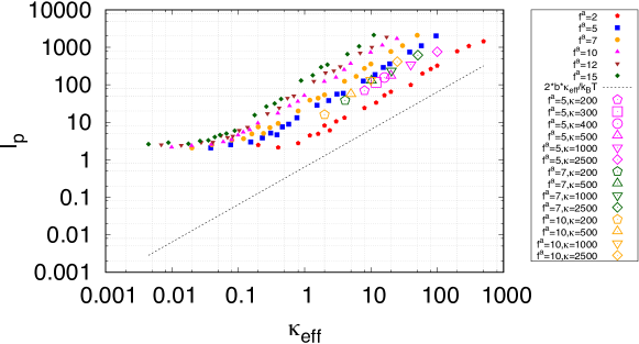
Figure S3: Effective persistence length $l_{\text{p}}$ estimated from the spectrum of filament tangent fluctuations in systems of isolated filaments (small filled symbols) and bulk active nematics (large open symbols). The dashed line has the slope of the expected scaling $2b\kappa_{\text{eff}}/k_{\text{B}}T$. We see that all results scale with the bare bending rigidity, $l_{\text{p}}\thicksim\kappa$, but only the results for the bulk systems exhibit data collapse for different activity strengths. The legend shows the value of $\kappa$ and ${f^{\text{a}}}$ for each system, and other parameters are $\tau_{1}=\tau$ and $k_{\text{b}}=30k_{\text{B}}T_{\text{ref}}/\sigma^{2}$.

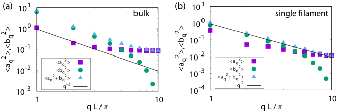
Figure S4: Fourier amplitudes $\langle a_{q}^{2}\rangle$, $\langle b_{q}^{2}\rangle$ and $\langle a_{q}^{2}+b_{q}^{2}\rangle$ as a function of wave vector $qL/\pi$, with $L$ the box side length, measured in a simulation of (a) a bulk simulation and (b) an isolated filament, for representative parameter values ($\kappa=500$,${f^{\text{a}}}=10$;$\kappa_{\text{eff}}=5$).

S5 Splay and bend deformations

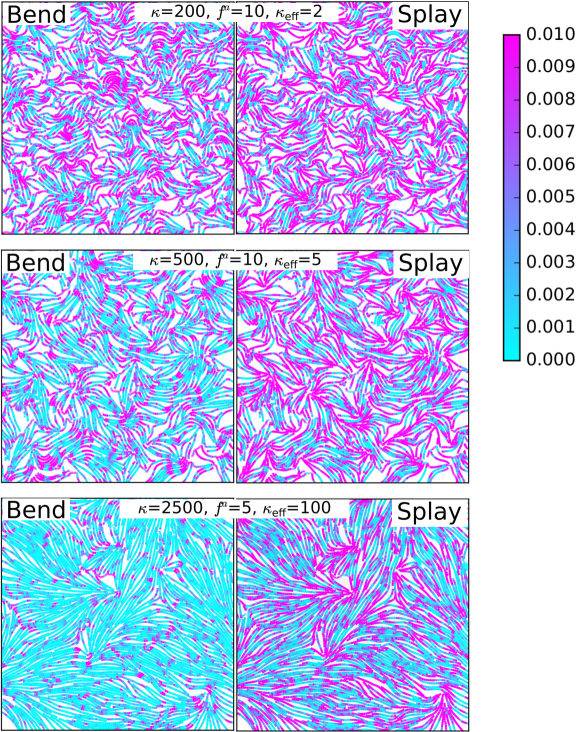
Figure S5: Snapshots from steady state configurations at indicated parameter values, with colormaps showing the distribution of bend, $\rho S^{2}(\hat{n}\times(\nabla\times\hat{n}))^{2}$ (left), and splay, $\rho S^{2}(\nabla\cdot\hat{n})^{2}$ (right), superposed on lines representing the director field. The parameters are chosen to highlight differences between flexible (small $\kappa_{\text{eff}}$)and rigid (large $\kappa_{\text{eff}}$) systems. The color range is clipped at 0.01 to to clarify the spatial variations of the deformations.

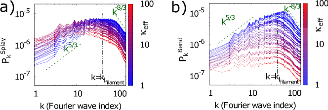
Figure S6: Power spectrum of splay (a) and bend (b) deformations as a function of wavenumber $k$, with the colorbar indicating the value of effective bending rigidity ($\kappa_{\text{eff}}$).

In a continuum description of a 2D nematic, all elastic deformations can be decomposed into bend and splay modes, given by $\mathbf{d}_{\text{bend}}(\mathbf{r})=\left(\hat{n}(\mathbf{r})\times(\nabla\times\hat{n}(\mathbf{r})\right)$ and $d_{\text{splay}}(\mathbf{r})=\left(\nabla\cdot\hat{n}(\mathbf{r})\right)$. Fig. S5 shows the spatial distribution of bend and splay deformations in systems at low and high rigidity values. To avoid breakdown of these definitions within defect cores or other vacant regions, we have normalized the deformations by the local density and nematic order: $D_{\text{bend}}=\rho S^{2}|\mathbf{d}_{\text{bend}}|^{2}$ and $D_{\text{splay}}=\rho S^{2}d_{\text{splay}}^{2}$. We see that bend and splay are equally spread out in the system in the limit of low rigidity, whereas bend deformations are primarily located near defect cores for large rigidity. In the high rigidity simulations, the effective persistence length ($\approx 66\sigma$) significantly exceeds the filament contour length ($20\sigma$), and thus most bend deformations correspond to rotation of the director field around filament ends at a defect tip.

To obtain further insight into the spatial organization of deformations, we calculated power spectra as $P^{\text{bend}}_{k}=\int d^{2}\mathbf{r}^{\prime}\exp\left(-i\mathbf{k}\cdot(\mathbf{r}^{\prime})\right)\langle D_{\text{bend}}(\mathbf{r})D_{\text{bend}}(\mathbf{r}+\mathbf{r}^{\prime})\rangle$, with an analogous definition for splay, and with the $Q$ field calculated at $1000\times 1000$ grid points (a realspace gridspacing of $0.84\sigma$). The resulting power spectra are shown in Fig. S6a,b as functions of the renormalized filament rigidity, and the dependences of the peak positions and maximal power are discussed in the main text. Here we note that the splay spectra exhibit asymptotic scaling of $k^{5/3}$ and $k^{-8/3}$ at scales respectively above the defect spacing or below the size of individual filaments, with a plateau region at intermediate scales. The same assymptotic scalings in power spectra were observed in dense bacterial suspensions in the turbulent regime Wensink et al. (2012); Chatterjee et al. (2016).

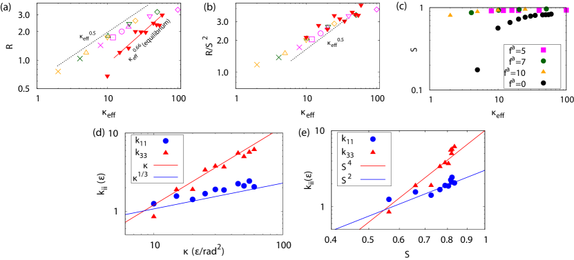
Figure S7: Comparison of ratio of bend and splay deformations in an active nematic to an equilibrium system. (a) The ratio of splay and bend deformations, $R$, plotted as a function of renormalized bending rigidity for active and equilibrium systems. The ratio $R$ calculated in equilibrium systems is shown as $\blacktriangledown$ symbols, while the symbols for the active system are defined as in Fig. S1. (b) The data from (a) is shown normalized by the mean nematic order parameter squared, (${\emph{R}}/S^{2}$). (c) The mean nematic order parameter, $S$, as a function of renormalized bending rigidity measured in active and equilibrium simulations. (d) Values of the bend ($k_{33}$) and splay ($k_{11}$) elastic constants as a function of $\kappa$ calculated using free energy perturbation Joshi et al. (2014) in equilibrium simulations (${f^{\text{a}}}=0$). (e) The same results as in (d), plotted against the nematic order parameter $S$ calculated for each parameter value. The red and blue lines indicate scaling of $\sim S^{4}$ and $\sim S^{2}$. The active results in this figure correspond to the additional data set with $k_{\text{b}}=30$ and $\tau_{1}=1$, as in Fig. S1.

The main text discusses the ratio of total strain energy in splay deformations to those in bend

$${\emph{R}}=\left\langle\int d^{2}\mathbf{r}D_{\text{splay}}(\mathbf{r})\right\rangle/\left\langle\int d^{2}\mathbf{r}D_{\text{bend}}(\mathbf{r})\right\rangle.$$ (S9)

We find that this ratio scales as ${\emph{R}}\thicksim\kappa_{\text{eff}}^{1/2}$ for all parameter sets, which is different from the expected scaling in an equilibrium nematic of ${\emph{R}}_{\text{eq}}\thicksim\kappa^{2/3}$. To investigate the origins of this discrepency, we measured the elastic moduli for an equilibrium system for different $\kappa$ values shown in Fig. (S7). We find that the degree of order in the system depends on the value of $\kappa$, that approximate scalings can be identified as $k_{33}\sim S^{4}$ and $k_{11}\sim S^{2}$ (Fig. (S7b)), and that the amount of order in the system at a given stiffness value $\kappa_{\text{eff}}$ is very different for active nematics when compared to their equilibrium analogs (Fig. (S7c)). Active nematics have considerably higher order, possibly because their intrinsic tendency to phase separate Mishra and Ramaswamy (2006); Chaté et al. (2006) leads to higher local density in comparison to an equilibrium system at corresponding $\rho$ and $\kappa_{\text{eff}}$. We used this information to empirically find that ${\emph{R}}/S^{2}$ exhibits approximately the same scaling for active and passive nematics.

Finally, by analogy to equipartition at equilibrium, the ratio of splay/bend, $R$, can be construed as an effective ratio of moduli: $k_{33}^{\text{effective}}/k_{11}^{\text{effective}}$, with the ratio depending on activity. Fig. S8 shows the defect shape parameter plotted as a function of this ratio.

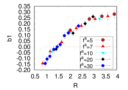
Figure S8: Defect shape parameter $b_{1}$ as a function of splay/bend ratio $R$ defined in the text, for the data in Fig. 3b,c of the main text.

S6 Testing the scaling form for the effective bending rigidity

Fig.  S9 shows two alternative scaling forms for the activity-renormalized bending rigidity $\kappa_{\text{eff}}$, with data from a wide range of activity values ($({f^{\text{a}}})^{2}\in[25,900]$). We see that only the form presented in the main text, $\kappa_{\text{eff}}\cong\kappa/{f^{\text{a}}}^{2}$ (Fig. 3 main text) leads to data collapse from simulations with different activity levels.

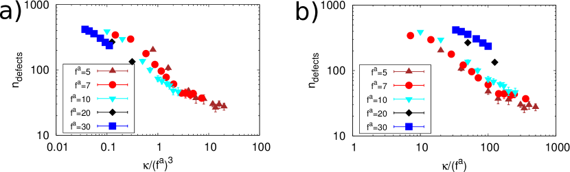
Figure S9: The data from Fig. 3 (main text) for defect densities measured in simulations at varying $\kappa$ and ${f^{\text{a}}}$ is plotted according to two alternative scaling forms for the activity-renormalized bending rigidity: (a) $\kappa_{\text{eff}}=\kappa/({f^{\text{a}}})^{3}$ and (b) $\kappa_{\text{eff}}=\kappa/{f^{\text{a}}}$.

S7 System size effects

To assess finite size effects on our results, we performed a system size analysis for two parameter sets from Fig. S1: $\kappa=200,{f^{\text{a}}}=5$ and $\kappa=2500,{f^{\text{a}}}=5$, with $\tau_{1}=\tau$ and $k_{\text{b}}=30$. We chose these parameter sets because they are near the upper and lower limits of effective bending rigidity investigated in that set of simulations. As shown in Fig. S10, we observe no systematic dependence of defect density on system size over the range of side lengths $L\in[200,1200]\sigma$. We observe a similar lack of dependence on system size for other observables, suggesting that finite size effects are negligible in our simulations at system size ($840\times 840\sigma^{2}$).

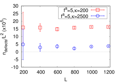
Figure S10: Steady-state defect density as a function of simulation box side length $L$ for square boxes with periodic boundary conditions, at indicated values of the filament modulus and activity parameter, with $\tau_{1}=\tau$ and $k_{\text{b}}=30k_{\text{B}}T_{\text{ref}}$.

S8 Density fluctuations

It is well-known that active nematics are susceptible to phase separation Mishra and Ramaswamy (2006); Ngo et al. (2014); Putzig and Baskaran (2014); Shi and Ma (2013) and giant number fluctuations (GNFs) Ramaswamy et al. (2003); Mishra and Ramaswamy (2006); Chaté et al. (2006); Narayan et al. (2007); Zhang et al. (2010). We therefore monitored these quantities in our system. Interestingly, while we do observe large density fluctuations on small scales (see videos of typical trajectories), phase separation is suppressed on large scales in the semiflexible regime. Fig. S11 shows histograms of local density, measured within subsystems with side length $10\sigma$ as a function of $\kappa$. We see that the distribution of local densities broadens as ${f^{\text{a}}}$ and $\kappa$ increase, but remains unimodal indicating an absence of true phase separation.

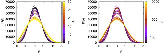
Figure S11: The distribution of local densities of filament pseudoatoms for indicated values of activity (left) and bare bending rigidity (right). Local densities were calculated by measuring the number of filament beads within square subsystems with side length $10\sigma$.

We also monitored the existence of GNFs, by measuring the number of pseudoatoms within square subsystems with side lengths ranging from $20\sigma$ to $840\sigma$ as a function of time. At equilibrium, in a region containing on average $N$ particles the standard deviation of the number of particles $\Delta N$ scales as $\Delta N\thicksim\sqrt{N}$, while previous studies of active nematics have identified higher scaling, as large as $\Delta N\thicksim N$. Consistent with the other characteristics of an active nematic studied in this article, we find that the scaling of number fluctuations depends only on the effective bending modulus $\kappa_{\text{eff}}$. Fig. S12a shows measured number fluctuations for different values of the effective bending modulus, plotted as $\Delta N/\sqrt{N}$, so that the result will be constant with subsystem size for a system exhibiting equilibrium-like fluctuations. We see that for small $\kappa_{\text{eff}}=2$ the result is constant with subsystem size, indicating equilibrium-like fluctuations, but the slope increases for $\kappa_{\text{eff}}=10$ and $\kappa_{\text{eff}}=100$ indicating a progression toward GNFs. At all $\kappa_{\text{eff}}$ the fluctuations are eventually suppressed on scales comparable to the defect spacing ($N\gtrsim 10^{4}$), at which scale the system is essentially isotropic, consistent with Narayan et al. Narayan et al. (2007).

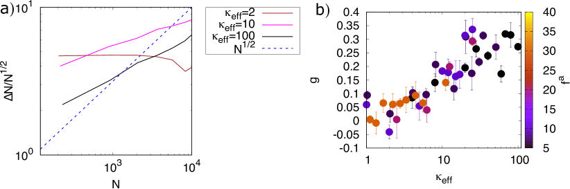
Figure S12: Giant number fluctuations (GNFs) depend on the renormalized bending rigidity. (a). The mean fluctuations of number of filament pseudoatoms, $\Delta N$, is plotted as a function of subsystem size $N$ for representative values of $\kappa_{\text{eff}}$. The fluctuations are normalized by their value at equilibrium, $\Delta N/\sqrt{N}$ so that a horizontal line indicates equilibrium-like fluctuations. (b) The fluctuation scaling exponent $g$ is plotted as a function of $\kappa_{\text{eff}}$. We determined $g$ by fitting the dependence of fluctuations on subsystem size for each parameter set to the form $\Delta N/\sqrt{N}=aN^{g}$ over the range $N\leq 10^{4}$. Note that a value of $g=0$ corresponds to equilibrium-like fluctuations, while $g=0.5$ would correspond to $\Delta N\thicksim N$.

To determine the dependence on $\kappa_{\text{eff}}$, we fit the data for each simulation in the range $N\leq 10^{4}$ to the form $aN^{g}$, so that $g=0$ indicates equilibrium-like fluctuations and $g=0.5$ would indicate linear scaling of fluctuations with system size. As shown in Fig. S12b, $g$ increases with $\kappa_{\text{eff}}$, with $g=0$ for small $\kappa_{\text{eff}}$ and $g\approx 0.3$ for the largest renormalized bending rigidity values investigated; i.e. $\Delta N\thicksim N^{0.8}$. The fact that $g<0.5$ for the parameters we consider may reflect suppression of fluctuations even for $N<10^{4}$. Importantly, estimated values of $g$ at different ${f^{\text{a}}}$ and $\kappa$ collapse onto a single function of $\kappa_{\text{eff}}$, consistent with the observations of other characteristics (Fig. 3 in the main text). We speculate that we do not observe GNFs for small renormalized bending rigidity values because GNFs are suppressed on scales beyond the defect spacing.

S9 Defect identification and shape measurement algorithm

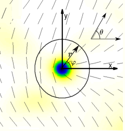
Figure S13: Schematic showing the defect-centered coordinate system defined in the text, with azimuthal angle $\phi$ and director angle $\theta(r,\phi)$. Note that the $x$-axis is chosen along the orientation vector of the +1/2 defect given by the angle $\theta_{0}^{\prime}$ defined in the text.

Here, we provide details on how we identify and measure the shapes of defects from our simulation data. This algorithm can also be directly applied to retardance images from experimental systems, and discretized output from continuum simulations.

Locating and identifying defects: We locate defects using the fact the magnitude of nematic order $S$ is very small at defect cores. We first compute the magnitude $S=2\sqrt{Q_{xx}^{2}+Q_{xy}^{2}}$ from the nematic tensor, whose measurement was described above. The regions corresponding to defect cores can then be extracted by using a flood-fill algorithm to select connected areas where the order is below some threshold $S_{\text{threshold}}$. We set $S_{\text{threshold}}=0.6$ since the system is deep within the nematic state for the parameters of this study. Once the defect cores have been located, the charge of each defect can be identified from the total change in the orientation of the director in a loop around the defect core. We perform this calculation by adding the change in angle for points in a circle about the center of the core. We choose the radius of the circle to be at least $5\sigma$, to ensure a well defined director field. The total change in angle must be a multiple of $\pi$: $\Delta\theta=n\pi$, where if $n=0$ then the disordered region is not a defect, and otherwise it is a defect with topological charge $m=\frac{n}{2}$. Typically $n=\pm 1$ but, in rare cases we observed defects with charge $m=+1$ in our simulation data.

Identifying the orientations and characterizing the shapes of $+\frac{1}{2}$ defects: Given the location of a defect and its charge, there are several methods which can be used to measure the orientation of the $+\frac{1}{2}$ defects DeCamp et al. (2015); Vromans and Giomi (2015). In this work, we compute the sum of the divergence of ${\bf Q}$ field, $\nabla_{\beta}Q_{\alpha\beta}$ along a circle enclosing the defect, and normalize it to a give unit vector. This unit vector represents the orientation of the +1/2 defect and in our two dimensional system identifies an angle $\theta^{\prime}_{0}$ for the defect.

We then measure the director orientation $\bar{\theta}(\bar{\phi})$ along the azimuthal angle $\bar{\phi}$ at discrete set of radii, $\{r\}$, around the defect core. First, we ensure that each loop does not cross any disordered regions, or enclose any other defects, by checking the order at each point and summing $\Delta\theta$ over the loop. Then we apply a coordinate frame rotation such that $\theta=\bar{\theta}-\theta^{\prime}_{0}$, and the azimuthal angle $\phi=\bar{\phi}-\theta^{\prime}_{0}$, where, $\theta^{\prime}_{0}$ is an orientation of the +1/2 defect estimated above. This step rotates the coordinate frame of reference to the frame of reference of the +1/2 defect. Finally, we evaluate the Fourier coefficients for $\theta(\phi)$,

$$\theta(r,\phi)=+\frac{1}{2}\phi+\sum_{n}a_{n}(r)\cos(n\phi)+b_{n}(r)\sin(n\phi).$$ (S10)

However, in practice we find that truncating the expansion after the first sin term gives an excellent approximation of the shape of a $+\frac{1}{2}$ defect. Hence, once a value of $r$ is chosen, the defect can be characterized by the single parameter $b_{1}$.

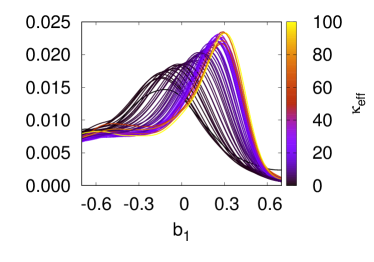
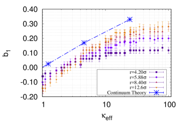
Figure S14: (left) Normalized distributions of $b_{1}$ obtained from the simulations in Fig. 3 (main text), with parameterizations calculated at a distance $r=12.6\sigma$ from the center of each defect according to Eq. (S10). (right) Effect of varying $r$ (the distance from the center of the +1/2 defect core) on the defect shape parameter $b_{1}$. The mode of $b_{1}$ is shown as a function of $\kappa_{\text{eff}}$ for the simulations in Fig. 3 (main text), with indicated values of $r$.

In Fig. S14 we show the distribution of $b_{1}$ values obtained from our simulations with $r=12.6\sigma$. Note that we observe long tailed distributions of $b_{1}$ with tails in the $b_{1}<0$ regime. However, the distributions are sharply peaked with typical peak width $\sim 0.1$. Therefore we consider the mode of $b_{1}$ values as an appropriate measure of defect shape.

Choice of $r$: For an isolated defect, $b_{1}$ asymptotes once the distance from the defect center increases beyond the core size. However, as noted in Zhou et al. Zhou et al. (2017), in a system with finite defect density the defect shape should be parameterized as close to the defect center as possible to avoid distortion due to other defects. The typical defect core radius in our simulations (defined as the region in which the nematic order parameter $S<0.6$) is about $4\sigma$. The smallest defect spacing (at the highest defect density) in our simulations is about $40\sigma$. We therefore chose a radius $r=12.6\sigma$, where the nematic is highly ordered and the director is always well-defined, but distortions due to other defects are minimized. As shown in Fig. S14b the results are qualitatively insensitive to radius for $r>5$, although statistics become more limited for larger $r$. For consistency, the same radius should be chosen for all systems.

Breakdown at high ${f^{\text{a}}}$ and $\kappa$: As noted in the main text, the defect identification algorithm breaks down in systems with both extremely high activity and high bare bending rigidity (${f^{\text{a}}}\geq 20$ and $\kappa\gtrsim 5000$). Under these conditions the system exhibits density fluctuations on very short length scales (see Fig. S11 and the movie showing snapshots from a simulation trajectory with ${f^{\text{a}}}=30$ and $\kappa=10^{4}$). The defect algorithm cannot distinguish between configurations in which stiff rods trans-pierced these holes and actual defects. Therefore we have not measured defect densities for these parameter sets.

References

- Weeks et al. (1971) J. D. Weeks, D. Chandler, and H. C. Andersen, J. Chem. Phys. 54, 5237 (1971).
- Kremer and Grest (1990) K. Kremer and G. S. Grest, J. Chem. Phys. 92, 5057 (1990), http://dx.doi.org/10.1063/1.458541 .
- Plimpton (1995) S. Plimpton, J. Comput. Phys. 117, 1 (1995).
- Peruani et al. (2006) F. Peruani, A. Deutsch, and M. Bär, Phys. Rev. E 74, 030904 (2006).
- McCandlish et al. (2012) S. R. McCandlish, A. Baskaran, and M. F. Hagan, Soft Matter 8, 2527 (2012).
- Weitz et al. (2015) S. Weitz, A. Deutsch, and F. Peruani, Phys. Rev. E 92, 012322 (2015).
- Ginelli et al. (2010) F. Ginelli, F. Peruani, M. Bär, and H. Chaté, Phys. Rev. Lett. 104, 184502 (2010).
- Peruani et al. (2012) F. Peruani, J. Starruß, V. Jakovljevic, L. Søgaard-Andersen, A. Deutsch, and M. Bär, Phys. Rev. Lett. 108, 098102 (2012).
- Joshi et al. (2014) A. A. Joshi, J. K. Whitmer, O. Guzmán, N. L. Abbott, and J. J. de Pablo, Soft Matter 10, 882 (2014).
- Doi and Edwards (1988) M. Doi and S. Edwards, The Theory of Polymer Dynamics, International series of monographs on physics (Clarendon Press, 1988).
- Wensink et al. (2012) H. H. Wensink, J. Dunkel, S. Heidenreich, K. Drescher, R. E. Goldstein, H. Lowen, and J. M. Yeomans, Proc. Nat. Acad. Sci. U.S.A. 109, 14308 (2012), 1208.4239v1 .
- Chatterjee et al. (2016) R. Chatterjee, A. A. Joshi, and P. Perlekar, Phys. Rev. E 94, 022406 (2016), arXiv:1608.01142 .
- Mishra and Ramaswamy (2006) S. Mishra and S. Ramaswamy, Phys. Rev. Lett. 97, 090602 (2006).
- Chaté et al. (2006) H. Chaté, F. Ginelli, and R. Montagne, Phys. Rev. Lett 96, 180602 (2006).
- Ngo et al. (2014) S. Ngo, A. Peshkov, I. S. Aranson, E. Bertin, F. Ginelli, and H. Chaté, Phys. Rev. Lett. 113, 038302 (2014), arXiv:1312.1076 .
- Putzig and Baskaran (2014) E. Putzig and A. Baskaran, Phys. Rev. E 90, 042304 (2014), 1057984 .
- Shi and Ma (2013) X.-q. Shi and Y.-q. Ma, Nat. Comm. 4, 3013 (2013).
- Ramaswamy et al. (2003) S. Ramaswamy, R. A. Simha, and J. Toner, Europhys. Lett. 62, 196 (2003).
- Narayan et al. (2007) V. Narayan, S. Ramaswamy, and N. Menon, Science 317, 105 (2007).
- Zhang et al. (2010) H. P. Zhang, A. Be’er, E.-L. Florin, and H. L. Swinney, Proc. Natl. Acad. Sci. U. S. A. 107, 13626 (2010), http://www.pnas.org/content/107/31/13626.full.pdf .
- DeCamp et al. (2015) S. J. DeCamp, G. S. Redner, A. Baskaran, M. F. Hagan, and Z. Dogic, Nat. Mater. 14, 1110 (2015).
- Vromans and Giomi (2015) A. J. Vromans and L. Giomi, Soft Matter , 1 (2015), 1507.05588 .
- Zhou et al. (2017) S. Zhou, S. V. Shiyanovskii, H.-S. Park, and O. D. Lavrentovich, Nat. Commun. 8, 14974 (2017).