Geometric parametric instability in periodically modulated GRIN multimode fibers

Abstract

We present a theoretical and numerical study of light propagation in graded-index (GRIN) multimode fibers where the core diameter has been periodically modulated along the propagation direction. The additional degree of freedom represented by the modulation permits to modify the intrinsic spatiotemporal dynamics which appears in multimode fibers. More precisely, we show that modulating the core diameter at a periodicity close to the self-imaging distance allows to induce a Moiré-like pattern, which modifies the geometric parametric instability gain observed in homogeneous GRIN fibers.

I Introduction

Parametric resonance (PR) is a well-known instability phenomenon which occurs in systems whose parameters vary in a periodic fashion. A classical example is a pendulum whose length changes harmonically with time. Depending on the system parameters, the pendulum may be unstable and the amplitude of its oscillations may become unbounded. Another example is the formation of standing waves on the surface of a liquid enclosed by a vibrating receptacle, a process known as Faraday instability Faraday . Faraday instability manifests as pattern formation in several extended systems Cross93 and it has been studied in Bose-Einstein condensates Garcia99 ; Staliunas2002 , granular systems Moon2001 or chemical processes Petrov97 . In these cases, the periodic modulation of the parameters is produced by an external forcing. However, the periodic variation may be self-induced by natural oscillations of the system as well. The emerging dynamics has been termed as geometric parametric instability (GPI) Krupa2016 . Faraday instabilities and GPI can both be observed in fiber optics, which is a particularly interesting physical system for their study due to its simplicity. In nonlinear fiber optics, a continuous wave (CW) may be unstable, leading to the amplification of spectral sidebands. This effect is called modulation instability (MI) and is commonly associated to anomalous dispersion regime Agrawal , although it is also observed in normal dispersion regime in the presence of higher order dispersion pitois2003 , fiber birefringence Wabnitz88 or multiple spatial modes Guasoni2015 ; Dupiol:17:2 . A CW may also be unstable whatever the dispersion regime if a parameter of the system is varied periodically (an external periodic forcing is applied), leading to the observation of PR, which can coexist with standard MI in the same system Copie2016 ; Conforti:16 ; Copie2017review ; Mussot2017 . This external forcing can result from periodic amplification Matera:93 , dispersion Armaroli:12 ; RotaNodari2015 ; Finot:13 ; Droques2013 ; Droques:12 or nonlinearity Abdullaev97 ; Staliunas2013 . The periodic evolution of nonlinearity can be self-induced, for example, in highly multimode GRIN fibers. Indeed, such fibers exhibit a periodic self-imaging of the injected field pattern due to the interference between the different propagating modes soldano1995 . This is due to the fact that the propagation constants of the modes are equally spaced and they have almost identical group velocity Mafi2012 . This creates a periodic evolution of the spatial size of the light pattern and therefore induces a periodic evolution of the effective nonlinearity in the propagation direction Wright2015b ; Conforti2017 . Recent experiments showed that PRs produced by this GPI can reach detunings from the pump in the order of hundreds of THz Krupa2016 .

In the present work, we study GPI in a system having an internal and external forcings with close but not equal periodicity. We consider a multimode GRIN fiber supporting self-imaging (at the origin of the internal forcing), with an additional modulation of the core diameter (inducing the external forcing). The overall longitudinal evolution of the spatial pattern exhibits two spatial frequencies, which can induce a Moiré-like effect. This results in the generation of characteristic spectral components which differ form the usual PR frequencies.

The outline of the paper is as follows. After this Introduction, in section II we report numerical simulations illustrating the self-imaging pattern and the parametric instability spectrum for a modulated GRIN fiber. In section III, we calculate the CW evolution of the beam along the propagation coordinate, characterized by two spatial periods. In section IV, we study the parametric instabilities generated by the spatial pattern when group velocity dispersion is considered, and provide estimates for the frequency of unstable bands. We draw our conclusions in V.

II Parametric instability in periodic GRIN fibers

Spatiotemporal light propagation in multimode GRIN fibers can be described by the following generalized nonlinear Schrödinger equation (GNLSE) Krupa2016 ; Longhi2003 :

$$i\partial_{z}E=\frac{1}{2\beta_{0}}\nabla_{\bot}^{2}E-\frac{\beta_{2}}{2}\partial^{2}_{t}E-\frac{\beta_{0}g(z)}{2}r^{2}E+\chi|E|^{2}E,$$ (1)

where $E$ is the electric field envelope measured in $\sqrt{\mathrm{W}}$/m, $\nabla_{\bot}^{2}$ is the Laplacian over the transverse coordinates, $r^{2}=x^{2}+y^{2}$, $\beta_{0}=k_{0}n_{0}$, $n_{0}$ being the refractive index at the core center, $k_{0}$ the vacuum wavenumber at the carrier frequency $\omega_{0}$, $\beta_{2}$ is the group velocity dispersion (GVD), $g(z)=2\Delta/\rho_{c}^{2}(z)$, where $\rho_{c}(z)$ is the fiber core radius and $\Delta$ is the relative refractive index difference between core and cladding ($\Delta=(n_{0}^{2}-n_{clad}^{2})/(2n_{0}^{2})$), and $\chi=\omega_{0}n_{2}/c$ is the nonlinear coefficient. We approximate the refractive index profile by $n^{2}(x,y,z)=n^{2}_{0}(1-2\Delta r^{2}/\rho_{c}(z)^{2})$, so that the waveguide is modeled as pure harmonic potential with a depth varying along $z$. In the following, we restrict our study to light propagation over short distances (a few centimeters), so that linear coupling between modes due to fiber imperfections can be disregarded. Moreover, we assume to excite the fiber with a Gaussian beam at the center so that the field presents circular symmetry. This allows to solve Eq. (1) by means of a split-step Fourier method Agrawal in cylindrical coordinates Guizar-Sicairos04 , significantly reducing the numerical integration time.

We start by considering a uniform commercial GRIN fiber, whose parameters are reported in the caption of Fig. 1. By injecting into this fiber a Gaussian beam of size $a_{0}=20~{}\mu$m at a wavelength $\lambda_{0}=1064$ nm, a periodic light pattern is generated with a period $\xi=\pi/\sqrt{g_{0}}\approx 600~{}\mu$m ($g_{0}=2\Delta/\rho_{0}^{2}$). This can be observed in Fig. 1(a), which shows the evolution of the intensity in the core center $I(z)=|E(z,x=0,y=0)|^{2}$ (normalized to the input one) as a function of fiber length (normalized to the self-imaging period $\xi$). Figure 1(b) shows the output spectrum obtained at a normalized distance of 16, which exhibits three distinct GPI sidebands in the range 100 - 220 THz detuning from the pump. We then consider the propagation of the same input beam in a modulated fiber, with a period $L_{mod}$ of 700 $\mu$m and a modulation depth of 3 $\mu m$. Figure 1(c) shows that the varying core diameter induces an additional modulation of the light intensity along the propagation. The self-imaging pattern is now modulated by an envelope of longer period $L$. As we will see hereafter, $L$ depends on the relation between the natural self-imaging period ($\xi$) and modulation period ($L_{mod}$). In the present example, $L_{mod}$ is chosen to be close to $\xi$ and the resulting dynamics may be understood as a kind of Moiré pattern. As shown in Fig. 1(d), this double periodicity in the spatial behaviour produces new spectral bands around those obtained with a uniform fiber, in a similar fashion to what was observed in a single-mode dispersion-oscillating fiber with doubly periodic dispersion Copie:15 . The process leading to the generation of these new spectral components will be analyzed and explained in the following sections.

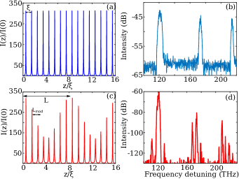
Figure 1: Results obtained from direct numerical simulation of GNLSE (1). (a,c) Evolution of the intensity in the core center normalized to the input one, versus fiber length normalized to the self-imaging period $\xi$ in a fiber with (a) uniform core and (c) varying core. (b,d) Output spectrum in a fiber with (b) uniform core and (d) varying core. Parameters typical of commercially available GRIN fibers: $n_{0}=1.47$, $n_{2}=3.2\times 10^{-20}$m²/W, $\rho_{0}=26~{}\mu$m, $\Delta=8.8\times 10^{-3}$, $\lambda_{0}=1064$ nm, $a_{0}=20~{}\mu$m, fiber length (b) 1.4 cm (d) 3 cm, $I_{0}$=20 GW/cm² and $\beta_{2}=16.55\cdot 10^{-27}$ s²/m.

III Calculation of the self-imaging pattern

To compute the spatial evolution of the beam profile, we start from Eq. (1) assuming CW propagation ($\partial_{t}=0$):

$$i\partial_{z}E=\frac{1}{2\beta_{0}}\nabla_{\bot}^{2}E-\frac{\beta_{0}g(z)}{2}r^{2}E+\chi|E|^{2}E.$$ (2)

An approximated solution of Eq. (2) in the weakly nonlinear regime, is a Gaussian beam with parameters varying along the propagation coordinate, which can be calculated by exploiting the method of moments PerezGarcia2000 or variational techniques Karlsson:91 . The solution reads as:

$$|E_{s}(x,y,z)|^{2}=A_{0}^{2}\left(\frac{a(z)}{a_{0}}\right)^{2}\text{exp}\left(-\frac{r^{2}}{a(z)^{2}}\right),$$ (3)

where $a(z)$ is the solution of the following equation (dot stands for $z$ derivative):

$$\ddot{a}+g(z)a+\frac{C}{a^{3}}=0,\quad C\equiv\left(\frac{n_{2}a_{0}^{2}A_{0}^{2}}{2n_{0}}-\frac{1}{\beta_{0}^{2}}\right).$$ (4)

The whole dynamics is thus ruled by the beam radius $a(z)$. Equation (4) is a singular nonlinear Hill equation of Ermakov type whose solution can be written as Pinney1950 ; Carinena2008 :

$$a(z)=\sqrt{u(z)^{2}-\frac{Cv(z)^{2}}{W^{2}}},$$ (5)

where $u(z),v(z)$ are two linearly independent solutions of the equation:

$$\ddot{x}+g(z)x=0,$$ (6)

$W=u\dot{v}-\dot{u}v=const.$ is the Wronskian, and the initial conditions are $u(0)=a_{0}$, $\dot{u}(0)=\dot{a}(0)$, $v(0)=0$ and $\dot{v}(0)\neq 0$. The linear Hill equation (6) is solvable in closed form only for very particular forms of $g(z)$ Nayfeh1995 . We consider here an harmonic modulation of the fiber core $\rho(z)=\rho_{0}(1+\delta\cos(kz))$, where $\delta$ describes the amplitude and $k=2\pi/L_{mod}$ the period of modulation.

In the $(L_{mod},\delta)$ plane, there are regions (known as Arnold tongues) where solutions of Eq. (6) becomes unbounded. This instability stems from the fact that the natural spatial frequency $k_{nat}\equiv\sqrt{g_{0}}=\sqrt{2\Delta}/\rho_{0}$ of the oscillator described by Eq. (6) is varied periodically with wavenumber $k$. The tips of the Arnold tongues fulfill the parametric resonance condition $k_{nat}=m\cdot k/2$ ($m$ integer), i.e. the natural spatial frequency is multiple of half the wavenumber of the spatial forcing, which gives the following condition on the ratio between modulation period and self-imaging distance:

$$L_{mod}=m\,\xi,\quad m=1,2,\ldots$$ (7)

When condition (7) is not satisfied, the evolution of the beam size is periodic (or quasi-periodic) Nayfeh1995 . Moreover, even if the condition (7) is satisified, there is a threshold on the modulation depth $\delta$ for the emergence of parametric instability, which in general increases for higher order resonances. For the rest of the paper we assume to be in absence of spatial parametric resonances.

Depending on the ratio between the modulation and self-imaging period, we can recover three different situations: $L_{mod}\ll\xi$, $L_{mod}\approx\xi$ and $L_{mod}\gg\xi$. The first case is the less interesting: in fact, the fast oscillating terms in Eq. (6) can be averaged out, and the beam evolves as in a uniform fiber. The other two cases present quite peculiar behaviors, which are analyzed in details below.

III.1 Moiré pattern: $L_{mod}\approx\xi$

The most interesting case rises when $L_{mod}\approx\xi$ and the modulation depth $\delta$ is small enough to avoid unbounded evolution. By assuming a small modulation amplitude $\delta\ll 1$, and expanding $1/\rho(z)$ at second order in the small parameter $\delta$, Eq. (6) takes the following form:

$$\ddot{x}+\frac{2\Delta}{\rho_{0}^{2}}(1-2\delta\cos(kz)+3\delta^{2}\cos^{2}(kz))x=0.$$ (8)

Two independent approximate solutions of Eq. (8) can be found by using multi-scale techniques (see appendix A):

$$u(z) =\frac{(4g_{0}-k^{2})a_{0}}{(4+2\delta)g_{0}-k^{2}}\left(\cos(\sqrt{g_{0}}\sigma z)+\frac{\delta g_{0}}{k}\left(\frac{\cos((\sqrt{g_{0}}\sigma-k)z)}{2\sqrt{g_{0}}-k}-\frac{\cos((\sqrt{g_{0}}\sigma+k)z)}{2\sqrt{g_{0}}+k}\right)\right),$$ (9)

$$v(z) =-B\left(\sin(\sqrt{g_{0}}\sigma z)+\frac{\delta g_{0}}{k}\left(\frac{\sin((\sqrt{g_{0}}\sigma-k)z)}{2\sqrt{g_{0}}-k}-\frac{\sin((\sqrt{g_{0}}\sigma+k)z)}{2\sqrt{g_{0}}+k}\right)\right),$$ (10)

where

$$W =-B\frac{(4g_{0}-k^{2})a_{0}}{(4+2\delta)g_{0}-k^{2}}\sqrt{g_{0}}\sigma,$$ (11)

$$\sigma =1+\frac{\delta^{2}(8g_{0}-3k^{2})}{4(4g_{0}-k^{2})},$$ (12)

and $B\neq 0$ is a constant, which does not appears in the expression of $a(z)$. Equations (9-10) gives the expression of the beam radius through Eq. (5). A comparison between the beam evolution obtained from Eqs. (9-10) and numerical solution of Eq. (4) is reported in Fig. 2, which shows a remarkable agreement. In general the solution is a combination of trigonometric functions of incommensurate arguments, an thus is not strictly periodic. For small enough core radius modulation, we can safely assume $\sigma\approx 1$. In this case, the spatial behaviour can be described as a combination of functions with period $\xi$ and functions with period $L_{mod}$. If we choose $L_{mod}$ and $\xi$ to be commensurate, the evolution of the beam is periodic with a longer period which verifies $L=pL_{mod}=q\xi$ ($p,q$ integers). In this regime, the resulting spatial behavior can be understood as a Moiré pattern, where two patterns with close periodicity $\xi$ and $L_{mod}$ are superimposed, giving birth to a new longer periodicity $L$. If $L_{mod}$ and $\xi$ are incommensurate, the evolution is only quasi-periodic. However, we can find $p,q$ that approximate the quasi-periodic evolution with periodic one with great accuracy. As we will illustrate below, the GPI spectrum resulting from a periodic or quasi-periodic evolution does not presents qualitative differences.

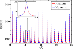
Figure 2: Evolution of the intensity in the core center calculated from numerical solution of Eq. (2) (blue curve) and exact solution (red curve) obtained from Eq. (3,5,9-10). Same parameters of Fig. 1(c).

III.2 Adiabatic modulation: $L_{mod}\gg\xi$

When $L_{mod}\gg\xi$, variations over the intensity are adiabatic, and we can use the Wentzel-Kramers-Brillouin (WKB) approximation Bender1999 to find two independent solutions $u(z),v(z)$ of Eq. (6), which inserted in Eq. (5) give the following expression for the beam size:

$$a(z)=\sqrt{a_{0}^{2}\sqrt{\frac{g(0)}{g(z)}}\cos^{2}(\phi(z))-\frac{C}{a_{0}^{2}\sqrt{g(0)g(z)}}\sin^{2}(\phi(z))}.$$ (13)

The phase $\phi(z)=\int_{0}^{z}dz^{\prime}\sqrt{g(z^{\prime})}$ reads as:

$$\phi(z) =\frac{2\sqrt{g_{0}}}{k\sqrt{1-\delta^{2}}}\left(\tan^{-1}\left[\sqrt{\frac{1-\delta}{1+\delta}}\tan\left(\frac{kz}{2}\right)\right]+\pi m\right),$$ (14)

$$m =\Big{\lfloor}\frac{z}{L_{mod}}+\frac{1}{2}\Big{\rfloor},$$

where $\lfloor x\rfloor=\max\{m\in\mathbb{Z}|m\leq x\}$. A comparison between the beam evolution obtained from Eqs. (13-14) and numerical solution of Eq. (4) is reported in Fig. 3, which shows a perfect agreement. We can see that the fast-varying self-imaging pattern of period $\xi$ is modulated adiabatically in a sinusoidal fashion by the longer period $L_{mod}$ ($L_{mod}=5\xi$ in this example). When the amplitude of modulation tends to 0 ($\delta\rightarrow 0$), the phase simplifies to $\phi(z)\approx\pi/\xi z$. In this limit, the spatial behavior can be again described as a combination of functions with period $\xi$ and functions with period $L_{mod}$. If $L_{mod}$ and $\xi$ are chosen to be commensurate, the evolution of the beam is periodic with a longer period which verifies $L=pL_{mod}=q\xi$, like the case where $L_{mod}\approx\xi$. In the general case, where $\delta\neq 0$ we observe a self-imaging pattern modulated by an envelope of period $L=L_{mod}$, which give rise to a quasi-periodic behavior.

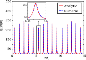
Figure 3: Evolution of the intensity at core center calculated from numerical solution of Eq. (4) (red dashed line) and analytical solution Eq. (13) (blue solid line) for $L_{mod}=5\xi$. Other parameters as in Fig. 1(c).

IV Linear stability analysis and GPI gain

We move now to the study of the stability of the CW spatial profile found in the previous section with respect to time periodic perturbations. We assume a spatiotemporal field of the form:

$$E(x,y,z,t)=(1+\delta E(z,t))E_{s}(x,y,z),$$ (15)

where $E_{s}$ is the approximated spatial electric field from Eq. (3) and $\delta E(z,t)$ is a small perturbation homogeneous in the transverse plane. By substituting ansatz (15) in Eq. (1), after linearization we obtain:

$$iE_{s}\partial_{z}\delta E=-\frac{\beta_{2}}{2}E_{s}\partial_{t}^{2}\delta E+\chi|E_{s}|^{2}E_{s}(\delta E+\delta E^{*}),$$ (16)

which projected on $E^{*}_{s}$, gives:

$$i\partial_{z}\delta E=-\frac{\beta_{2}}{2}\partial_{t}^{2}\delta E+\frac{\chi A_{0}^{2}a_{0}^{2}}{2a(z)^{2}}(\delta E+\delta E^{*}).$$ (17)

A similar equation can be obtained when studying MI in single mode fibers with oscillating nonlinearity Matera:93 ; RotaNodari2015 ; Abdullaev97 ; Armaroli:12 . By considering a time harmonic perturbation of the form $\delta E=a(z)e^{i\Omega t}+b^{*}(z)e^{-i\Omega t}$, we get the following system:

$$\begin{bmatrix}\dot{a}\\ \dot{b}\end{bmatrix}=i\begin{bmatrix}\frac{\beta_{2}\Omega^{2}}{2}+F(z)&F(z)\\ -F(z)&-\left(\frac{\beta_{2}\Omega^{2}}{2}+F(z)\right)\\ \end{bmatrix}\begin{bmatrix}a\\ b\end{bmatrix},$$ (18)

where

$$F(z)=\frac{\chi A_{0}^{2}a_{0}^{2}}{2a(z)^{2}},$$ (19)

which can be reduced to a second order ordinary differential equation for $y=a+b$:

$$\ddot{y}+\frac{\beta_{2}\Omega^{2}}{2}\left(\frac{\beta_{2}\Omega^{2}}{2}+2F(z)\right)y=0.$$ (20)

Since we have restricted our analysis to bounded evolutions of $a(z)$, the function $F(z)$ is (quasi) periodic as discussed in previous section. In this case, Eq. (20) is again a Hill equation. Note that Eq. (20) rules the evolution of the time periodic perturbations, so that an unbounded evolution for $y$ implies the instability of the CW field. The values of the perturbation frequency $\Omega$ for which the evolution of $y$ becomes unbounded gives thus the GPI spectrum.

IV.1 Constant core diameter

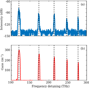
Figure 4: GPI gain for the uniform fiber case. (a) Output spectrum obtained by solving numerically GNLSE (1). Black dashed lines corresponds to unstable frequencies obtained from parametric resonance condition Eq. (24). (b) Floquet spectrum obtained from Eq. (18). Parameters: $A_{0}^{2}=$20 GW/cm², $a_{0}$ = 20 $\mu$m and fiber length 2.2 cm. Remaining parameters as in Fig. 1(a-b).

We start by considering a uniform fiber, which has already been studied in Longhi2003 . In this case the beam radius $a(z)$ assumes the following simple expression:

$$a^{2}(z)=a_{0}^{2}[\cos^{2}(\sqrt{g_{0}}z)+\mathcal{C}\sin^{2}(\sqrt{g_{0}}z)],$$ (21)

where $\mathcal{C}=(1-\mathcal{P})/(\beta_{0}^{2}a_{0}^{4}g_{0})=-C/(g_{0}a_{0}^{4})$ and $\mathcal{P}=n_{2}\beta_{0}^{2}A_{0}^{2}a_{0}^{2}/2n_{0}$ is a dimensionless parameter measuring the distance from beam collapse (here we assume $\mathcal{P}\ll 1$) Karlsson:91 ; Longhi2003 . Expression (21) is recovered by putting $\delta=0$ in Eqs. (5,9-10). The average value of $F(z)$ can be calculated as:

$$F_{av}=\frac{1}{\xi}\int_{0}^{\xi}F(z)dz=\frac{\chi A_{0}^{2}}{2\sqrt{\mathcal{C}}}.$$ (22)

The parametric resonance condition for Eq. (20), which reads:

$$\frac{\beta_{2}\Omega^{2}}{2}\left(\frac{\beta_{2}\Omega^{2}}{2}+2F_{av}\right)=\left(m\,\frac{\pi}{\xi}\right)^{2},$$ (23)

permits to find the central frequencies of the GPI bands as:

$$\Omega_{m}^{2}=\frac{2}{\beta_{2}}\left(-F_{av}+\sqrt{F_{av}^{2}+g_{0}\,m^{2}}\right),\quad m=1,2,\ldots$$ (24)

The full GPI spectrum can be calculated by means of Floquet theory. This consist in solving system (18) for two independent initial conditions (f.i. $[1,0]^{T}$ and $[0,1]^{T}$) over one period ($z=\xi$ in this case). This system can be solved only numerically because of the nontrivial form of $F(z)$. The two solutions calculated at $z=\xi$ compose the two columns of the $2\times 2$ Floquet matrix, whose eigenvalues $\mu_{1},\mu_{2}$ determine the stability of the CW solution. If one eigenvalue (say $\mu$) has modulus greater than one, the solution is unstable and the perturbations grow exponentially along $z$ with gain $G(\Omega)=\ln|\mu|/\xi$.

Figure 4 presents a comparison between the spectrum obtained from numerical solution of full GNLSE (1), starting from a CW perturbed by a small random noise, for 2.2 cm long uniform fiber [Fig. 4(a)], and the gain spectrum obtained from Floquet theory [Fig. 4(b)]. Vertical black dashed lines represent the frequencies $\Omega_{m}$ given by Eq. (24) for $m=1,\ldots,5$, which are in excellent agreement with the locations of maximum gain. Note that in the low intensity limit ($A_{0}\rightarrow 0$), they can be approximated as $\Omega_{m}^{2}\approx 2\pi m/(\xi\beta_{2})$ Krupa2016 . The gain spectrum obtained from Floquet theory, plotted in Fig. 4(b), is in excellent agreement with the spectrum obtained from direct numerical simulation, plotted in Fig. 4(a), concerning the frequency and width of the gain bands, as well as their relative intensity.

IV.2 Varying core diameter

When the core diameter varies periodically, the spatial dynamics becomes richer and the self-imaging pattern is modulated, as described by Eqs. (5,9-10) for $L_{mod}\approx\xi$, or Eqs. (13,14) for $L_{mod}\gg\xi$. As we will show in the following, this spatial dynamics generates additional GPI bands.

For the sake of simplicity, we consider a modulation period commensurate with the self imaging distance, i.e. $p\,L_{mod}=q\,\xi$ (where $p$ and $q$ are two integers). In this case the spatial evolution can be considered periodic with period $L=q\,\xi$, which allows us to obtain a simple analytic expression for the maxima of GPI gain. The parametric resonance condition for Eq. (20) reads now:

$$\frac{\beta_{2}\Omega^{2}}{2}\left(\frac{\beta_{2}\Omega^{2}}{2}+2F_{av}\right)=\left(m\,\frac{\pi}{L}\right)^{2},$$ (25)

where we have assumed that the average nonlinear forcing term $F_{av}$ is the same as in the case of the uniform fiber. It is convenient to write the integer as $m=m_{1}q+m_{2}$, which gives the following expression for the central frequencies of the GPI bands:

$$\Omega_{m_{1},m_{2}}^{2}=\frac{2}{\beta_{2}}\left(-F_{av}+\sqrt{F_{av}^{2}+g_{0}\left(m_{1}+\frac{m_{2}}{q}\right)^{2}}\right).$$ (26)

The index $m_{1}=0,1,\ldots$ counts the main resonances, which correspond to the ones obtained in the uniform case for $m_{2}=0,m_{1}\neq 0$ [see Eq. (24)]. The most important information which can be extracted from Eq. (26) is that we have the generation of new sidebands around the principal ones. The number $m_{2}$ describes these additional sub-harmonic resonances deriving from the longer modulation period $L>\xi$. The interval of values for $m_{2}$ depends on the parity of $q$, and is defined formally for $q$ even as:

$$q=2n\Rightarrow\left\{\begin{array}[]{rcc}-n+1&\leq m_{2}\leq n,&m_{1}\neq 0,\\ 1&\leq m_{2}\leq n,&m_{1}=0,\end{array}\right.$$ (27)

or odd as:

$$q=2n+1\Rightarrow\left\{\begin{array}[]{rcc}-n&\leq m_{2}\leq n,&m_{1}\neq 0,\\ 1&\leq m_{2}\leq n,&m_{1}=0.\end{array}\right.$$ (28)

For example we consider now a shallow modulation ($\delta=0.12$) of the fiber, with a period $L_{mod}=8/7\xi$. Figure 5(a) reports the spectrum after a propagation of 3 cm from numerical simulations of GNLSE (1). We can observe the characteristic splitting of bands due to the double periodicity. Black dashed lines show the frequency of unstable sidebands given by Eq. (24), which are in excellent agreement with the numerical simulation result. We can calculate the width and position of bands by performing a numerical Floquet analysis as described in the previous section. As in the constant core case, the frequency, width and relative intensity of the sidebands is in excellent agreement with numerical simulations (Fig. 5(a)).

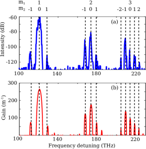
Figure 5: Modulated fiber case. (a) Output spectrum obtained by solving numerically GNLSE (1). Black dashed lines corresponds to unstable frequencies obtained from Eq. (26). (b) Floquet spectrum obtained from Eq. (18). Parameters: $\delta=0.12$, $L_{mod}=(8/7)\xi$, $A_{0}^{2}=20$ GW/cm² and fiber length 3 cm. Remaining parameters as in Fig. 1(a-b).

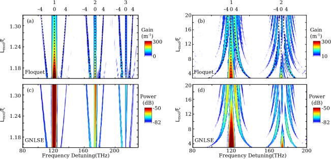
Figure 6: (a,b) Gain map obtained with numerical Floquet analysis as a function of the ratio $L_{mod}/\xi$, for (a) $L_{mod}\approx\xi$ and (b) $L_{mod}\gg\xi$. (c,d) Direct numerical integration of equation 2, for (c) $L_{mod}\approx\xi$ and (d) $L_{mod}\gg\xi$. Parameters: $\beta_{2}=16.55\times 10^{-27}$ s²/m, $a_{0}=20~{}\mu$m , $\rho_{0}=26~{}\mu$m and $A_{0}^{2}=20~{}GW/cm^{2}$

It is interesting to investigate the the gain spectrum as a function of the ratio $L_{mod}/\xi$ between the modulation period and the self-imaging distance. We start by considering the range $L_{mod}\approx\xi$, where the spatial Moiré pattern is generated. Figure 6(a) shows the GPI gain map as a function of frequency and modulation period, calculated by means of the Floquet theory described before, using expressions Eqs. (5,9-10) for the beam size. The corresponding ratio between periods has been chosen to be commensurate and verifies $L_{mod}=(n+16)/(n+12)\xi$, where $n$ is an integer in the interval $[0,20]$. The overall period of the spatial pattern is thus given by $L=(n+16)\xi$. A remarkable agreement is found with the unstable frequencies predicted by Eq. (24), which are reported in Fig. 6(a) as black dashed curves. For each principal resonance $m_{1}=1,2,3$, one can notice the generation of additional sideband pairs $m_{2}=\pm 4$, whose frequency separation increases with the modulation period. These additional sidebands pairs appear at index $m_{2}=\pm 4$ because, for the definition of the modulation period used in this example, each value of $n$ generates an overall period $L$ composed four slow oscillations (the pattern is quasi-periodic of period $\approx L/4$).

The other interesting case occurs when the modulation period of the core diameter is chosen to be several times greater than self-imaging distance, i.e. $L_{mod}\gg\xi$, where the spatial pattern is described by Eqs. (13,14). In this case, the relation between $L_{mod}$ and $\xi$ has been chosen to verify $L_{mod}=(12+n)/4\xi$, where now $n$ is taken in the interval $[0,68]$, giving an overall period $L=(n+12)\xi$. The corresponding Floquet gain map is reported in 6(b), where one can notice some qualitative differences. For the smallest modulation period, only a pair of sidebands appears, well detached from the fundamentals ones, corresponding to $m_{1}=1,2$. By increasing the modulation period, additional sidebands pairs stem out, and they all tends to cluster around the principal ones. For the longer modulation period considered here, at least three couples of sidebands merge with the fundamental ones, giving rise to a single structured band. Also in this case, a remarkable agreement is found with the unstable frequencies predicted by Eq. (24) (black dashed curves).

The results of Floquet analysis are essentially supported by direct numerical integration of Eq. (1), as evidenced by Figs. 6(c) and (d), which reports the output spectrum after a propagation distance of 3 cm as function of $L_{mod}$. In order to get rid of any randomness in the initial condition, we add a coherent seed to the CW (a short hyperbolic secant of duration 1 fs and intensity 10^-5 smaller than the cw pump). Moreover, $L_{mod}$ has been chosen to be equally spaced between the upper and lower limits considered, so the ratio $L_{mod}$ and $\xi$ are not necessary commensurate. This fact confirms that considering the spatial behavior as strictly periodic does not produce any qualitative difference.

V Conclusions

We have theoretically studied GPI in a graded-index multimode fiber with an axially-modulated core diameter. We have shown that a periodic modulation of the core diameter allows to generate new GPI sidebands. We have developed a theory to predict the frequency of these additional sidebands, which is in excellent agreement with direct numerical simulations of the GNLSE and Floquet stability analysis. In our simulations we have used realistic parameters, this fact gives a solid evidence the described effects can be experimentally observed. This study contributes to a further understanding of the rich dynamics related to nonlinear waves propagating in multimode fibers.

Appendix A Multiscale analysis

In this appendix, we give some details on the method used to approximate the beam evolution in the limit $L_{mod}\approx\xi$. We start from Eq. (8), where we define the dimensionless coefficients $w=\sqrt{g}/k$, $\epsilon=w^{2}\delta$ and $\bar{z}=kz$, to get:

$$\ddot{x}+\left(w^{2}-2\epsilon\cos(\bar{z})+\frac{3\epsilon^{2}}{w^{2}}\cos^{2}(\bar{z})\right)x=0.$$ (29)

The initial assumption $L_{mod}\approx\xi$ implies $w\approx 1$, thus we can safely perform a multiscale development in $\epsilon\ll 1$ Nayfeh1995 up to first order. By defining $\bar{z}_{n}=\epsilon^{n}\bar{z}$ and $x=\sum_{n=0}\epsilon^{n}x_{n}$, and equating equal powers of $\epsilon$, an infinite heriarchy of equations is obtained. From this infinite set equations, we retain only up to order $\epsilon^{2}$:

$$\epsilon^{0}:\quad(D^{2}_{0}+w^{2})x_{0} =0,$$ (30)

$$\epsilon^{1}:\quad(D^{2}_{0}+w^{2})x_{1} =-2(D_{1}D_{0}-\cos(\bar{z}_{0}))x_{0},$$ (31)

$$\epsilon^{2}:\quad(D^{2}_{0}+w^{2})x_{2} =-2(D_{1}D_{0}-\cos(\bar{z}_{0}))x_{1}-$$ (32)

$$-(2D_{2}D_{0}+D_{1}^{2}+\frac{3}{2w^{3}}\cos(\bar{z}_{0}))x_{0},$$

where $D_{n}=\partial_{\bar{z_{n}}}$. At order $\epsilon^{0}$, we find:

$$x_{0}=A(\bar{z}_{1},\bar{z}_{2})e^{iwz}+A^{*}(\bar{z}_{1},\bar{z}_{2})e^{-iwz}$$ (33)

where $A(\bar{z}_{1},\bar{z}_{2})$ is a complex function depending on the slower variables $\bar{z}_{1},\bar{z}_{2}$. To know the dependence of this fuction on $z_{1}$ and $z_{2}$, Eq. (33) is substituted in Eq. (31) and secular terms are imposed to vanish. We obtain the following solution for $x_{1}$:

$$x_{1}=A(\bar{z}_{2})\left(\frac{-e^{i(w+1)\bar{z}_{0}}}{2w+1}+\frac{e^{i(w-1)\bar{z}_{0}}}{2w-1}\right)+c.c$$ (34)

where c.c denotes complex conjugate. To find $A(\bar{z}_{2})$, we substitute $x_{1}$ in Eq. (32) and impose again secular terms to vanish, this bring us to:

$$A=\frac{C}{2}e^{i(\phi\bar{z}_{2}+\beta)}\quad,\quad\phi=\frac{8w^{2}-3}{4w^{3}(4w^{2}-1)},$$ (35)

where $C$ and $\beta$ are two real constants fixed by the boundary conditions. By writing the complete function $x=x_{0}+\epsilon x_{1}+O(\epsilon^{2})$ we obtain the general solution:

$$x=C\left[\cos(\tilde{w}z+\beta)+\epsilon\left(\frac{\cos((\tilde{w}-1)z+\beta)}{2w-1}-\frac{\cos((\tilde{w}+1)z+\beta)}{2w+1}\right)\right]+O(\epsilon^{2})~{},~{}\tilde{w}=w\left(1+\frac{\delta^{2}(8\omega^{2}-3)}{4(4\omega^{2}-1)}\right)$$ (36)

From this equation, we can readily obtain $u(z)$ an $v(z)$ by imposing the appropriate boundary conditions.

References

- (1) M. Faraday Philos. Trans. R. Soc. London, vol. 121, p. 319, 1831.
- (2) M. C. Cross and P. C. Hohenberg, “Pattern formation outside of equilibrium,” Rev. Mod. Phys., vol. 65, pp. 851–1112, Jul 1993.
- (3) V. M. García-Ripoll, Juan J andPérez-García and P. Torres, “Extended Parametric Resonances in Nonlinear Schrödinger Systems,” Phys. Rev. Lett., vol. 83, no. 9, pp. 1715–1718, 1999.
- (4) K. Staliunas, S. Longhi, and G. J. de Valcárcel, “Faraday Patterns in Bose-Einstein Condensates,” Phys. Rev. Lett., vol. 89, no. 21, p. 210406, 2002.
- (5) S. J. Moon, M. D. Shattuck, C. Bizon, D. I. Goldman, J. B. Swift, and H. L. Swinney, “Phase bubbles and spatiotemporal chaos in granular patterns,” Phys. Rev. E, vol. 65, p. 011301, Dec 2001.
- (6) V. Petrov, Q. Ouyang, and H. L. Swinney, “Resonant pattern formation in a chemical system,” Nature, vol. 388, p. 655, 1997.
- (7) K. Krupa, A. Tonello, A. Barthélémy, V. Couderc, B. M. Shalaby, A. Bendahmane, G. Millot, and S. Wabnitz, “Observation of Geometric Parametric Instability Induced by the Periodic Spatial Self-Imaging of Multimode Waves,” Phys. Rev. Lett., vol. 116, no. 18, p. 183901, 2016.
- (8) G. Agrawal, Nonlinear Fiber Optics. Elsevier, 2013.
- (9) S. Pitois and G. Millot, “Experimental observation of a new modulational instability spectral window induced by fourth-order dispersion in a normally dispersive single-mode optical fiber,” Optics Communications, vol. 226, no. 1, pp. 415 – 422, 2003.
- (10) S. Wabnitz, “Modulational polarization instability of light in a nonlinear birefringent dispersive medium,” Phys. Rev. A, vol. 38, pp. 2018–2021, Aug 1988.
- (11) M. Guasoni, “Generalized modulational instability in multimode fibers: Wideband multimode parametric amplification,” Phys. Rev. A., vol. 033849, pp. 1–14, 2015.
- (12) R. Dupiol, A. Bendahmane, K. Krupa, J. Fatome, A. Tonello, M. Fabert, V. Couderc, S. Wabnitz, and G. Millot, “Intermodal modulational instability in graded-index multimode optical fibers,” Opt. Lett., vol. 42, pp. 3419–3422, Sep 2017.
- (13) F. Copie, M. Conforti, A. Kudlinski, A. Mussot, and S. Trillo, “Competing turing and faraday instabilities in longitudinally modulated passive resonators,” Phys. Rev. Lett., vol. 116, p. 143901, Apr 2016.
- (14) M. Conforti, F. Copie, A. Mussot, A. Kudlinski, and S. Trillo, “Parametric instabilities in modulated fiber ring cavities,” Opt. Lett., vol. 41, no. 21, pp. 5027–5030, 2016.
- (15) F. Copie, M. Conforti, A. Kudlinski, A. Mussot, F. Biancalana, and S. Trillo, “Instabilities in passive dispersion oscillating fiber ring cavities,” The European Physical Journal D, vol. 71, p. 133, May 2017.
- (16) A. Mussot, M. Conforti, S. Trillo, F. Copie, and A. Kudlinski, “Modulation instability in dispersion oscillating fibers,” Advances in Optics and Photonics, p. to appear, 2017.
- (17) F. Matera, A. Mecozzi, M. Romagnoli, and M. Settembre, “Sideband instability induced by periodic power variation in long-distance fiber links,” Opt. Lett., vol. 18, pp. 1499–1501, Sep 1993.
- (18) A. Armaroli and F. Biancalana, “Tunable modulational instability sidebands via parametric resonance in periodically tapered optical fibers,” Opt. Express, vol. 20, no. 22, pp. 25096–25110, 2012.
- (19) S. R. Nodari, M. Conforti, G. Dujardin, A. Kudlinski, A. Mussot, S. Trillo, and S. De Bièvre, “Modulational instability in dispersion-kicked optical fibers,” Phys. Rev. A, vol. 92, no. 1, p. 13810, 2015.
- (20) C. Finot, J. Fatome, A. Sysoliatin, A. Kosolapov, and S. Wabnitz, “Competing four-wave mixing processes in dispersion oscillating telecom fiber,” Opt. Lett., vol. 38, pp. 5361–5364, Dec 2013.
- (21) M. Droques, A. Kudlinski, G. Bouwmans, G. Martinelli, and A. Mussot, “Dynamics of the modulation instability spectrum in optical fibers with oscillating dispersion,” Phys. Rev. A, vol. 87, p. 013813, Jan 2013.
- (22) M. Droques, A. Kudlinski, G. Bouwmans, G. Martinelli, and A. Mussot, “Experimental demonstration of modulation instability in an optical fiber with a periodic dispersion landscape,” Opt. Lett., vol. 37, pp. 4832–4834, Dec 2012.
- (23) F. K. Abdullaev, S. A. Darmanyan, S. Bischoff, and M. P. Sørensen, “Modulational instability of electromagnetic waves in media with varying nonlinearity,” J. Opt. Soc. Am. B, vol. 14, pp. 27–33, Jan 1997.
- (24) K. Staliunas, C. Hang, and V. V. Konotop, “Parametric patterns in optical fiber ring nonlinear resonators,” Phys. Rev. A, vol. 88, p. 023846, Aug 2013.
- (25) L. B. Soldano and E. C. M. Pennings, “Optical multi-mode interference devices based on self-imaging: principles and applications,” Journal of Lightwave Technology, vol. 13, no. 4, pp. 615–627, 1995.
- (26) A. Mafi, “Pulse Propagation in a Short Nonlinear Graded-Index Multimode Optical Fiber,” Journal of Lightwave Technology, vol. 30, p. 2803, 2012.
- (27) L. G. Wright, S. Wabnitz, D. N. Christodoulides, and F. W. Wise, “Ultrabroadband dispersive radiation by spatiotemporal oscillation of multimode waves,” Phys. Rev. Lett., vol. 115, p. 223902, Nov 2015.
- (28) M. Conforti, C. M. Arabi, A. Mussot, and A. Kudlinski, “Fast and accurate modeling of nonlinear pulse propagation in graded-index multimode fibers,” Opt. Lett., vol. 42, pp. 4004–4007, Oct 2017.
- (29) S. Longhi, “Modulational instability and space–time dynamics in nonlinear parabolic-index optical fibers,” Optics letters, vol. 28, no. 23, pp. 2363–2365, 2003.
- (30) M. Guizar-Sicairos and J. C. Gutiérrez-Vega, “Computation of quasi-discrete hankel transforms of integer order for propagating optical wave fields,” J. Opt. Soc. Am. A, vol. 21, pp. 53–58, Jan 2004.
- (31) F. Copie, A. Kudlinski, M. Conforti, G. Martinelli, and A. Mussot, “Modulation instability in amplitude modulated dispersion oscillating fibers,” Opt. Express, vol. 23, no. 4, pp. 3869–3875, 2015.
- (32) V. M. Pérez-García, P. Torres, J. J. García-Ripoll, and H. Michinel, “Moment analysis of paraxial propagation in a nonlinear graded index fibre,” Journal of Optics B: Quantum and Semiclassical Optics, vol. 2, no. 3, p. 353, 2000.
- (33) M. Karlsson, D. Anderson, M. Desaix, and M. Lisak, “Dynamic effects of Kerr nonlinearity and spatial diffraction on self-phase modulation of optical pulses,” Opt. Lett., vol. 16, no. 18, pp. 1373–1375, 1991.
- (34) E. Pinney, “The nonlinear differential equation ,” Proc. Amer. Math. Soc, vol. 1, p. 681, 1950.
- (35) J. F. Cariñena, “A new approach to Ermakov systems and applications in quantum physics,” The European Physical Journal Special Topics, vol. 160, no. 1, pp. 51–60, 2008.
- (36) A. H. Nayfeh and D. T. Mook, Nonlinear Oscillations. Wiley, 1995.
- (37) C. M. Bender and S. A. Orszag, Advanced Mathematical Methods for Scientists and Engineers. Springer, 1999.