A partial inverse problem for the Sturm-Liouville operator on the graph with a loop
Chuan-Fu Yang, Natalia P. Bondarenko
Abstract. The Sturm-Liouville operator with singular potentials on the lasso graph is considered.
We suppose that the potential is known a priori on the boundary edge, and recover the potential on the loop
from a part of the spectrum and some additional data. We prove the uniqueness theorem and provide a constructive algorithm
for the solution of this partial inverse problem.
Keywords: partial inverse spectral problem; Sturm-Liouville operator on a lasso graph; quantum graph; singular potential.
Differential operators on geometrical graphs, also called quantum graphs, are intensively studied by mathematicians in recent years,
and have applications in organic chemistry, mechanics, mesoscopic physics, nanotechnology, theory of waveguides and other branches
of science [1]. There is an extensive literature, devoted to quantum graphs. We mention here works [2, 3],
where the further references could be found. A nice elementary introduction to the theory of quantum graphs is provided in [4].
The recent paper [5] contains a good overview of results on inverse spectral problems for differential operators on graphs,
which consist in recovering differential operators (especially coefficients of differential expressions) from various types of spectral data.
In this paper, we consider the Sturm-Liouville operator on the graph with a loop. We suppose that the potential is known a priori on a part of the graph,
and recover the potential on the remaining part from a part of the spectrum and some additional data.
Such partial inverse problems have been studied in papers
[6, 7, 8, 9, 10, 11, 12] for star-shaped graphs.
In the present paper, we obtain the first results
in this direction for the graph with a loop. We formulate a partial inverse problem on a lasso graph (see Figure 1),
prove the uniqueness theorem and provide a constructive algorithm for solution of this problem.
Note that complete inverse problems for differential operators on lasso graphs were studied in [13, 14, 15].
We hope that in the future, our results will be generalized for graphs with a more complicated structure.
We develop the technique of [10, 11, 12], based on the Riesz basis property of some systems of vector functions.
We also mention that our problem on a graph is related to the Hochstadt-Lieberman problem on a finite interval [16].
The paper is organized as follows. In Section 2, we state the boundary value problem on the lasso graph and study asymptotic properties
of its eigenvalues. Section 3 is devoted to the periodic inverse Sturm-Liouville problem, which is further used as an auxiliary step for recovering
the potential on the loop. In Section 4, we formulate the partial inverse problem, provide our main results and proofs.
2. Asymptotic formulas for eigenvalues
Consider the lasso graph , represented in Figure 1. The edge is a boundary edge of length ,
the edge is a loop of length . Introduce a parameter for each edge , , .
The value corresponds to the boundary vertex, and corresponds to the internal vertex.
For the loop , both ends and correspond to the internal vertex.
Figure 1: Lasso graph
Let be a vector function on the graph .
Consider Sturm-Liouville expressions
on the edges of , where , , are real-valued functions from
. This means that , , where the derivative is understood in the sense of distributions.
We call the functions the potentials.
Define the quasi-derivatives , .
Then the differential expressions can be undrestood in the following sense:
on the domain
Inverse problems for Sturm-Liouville operators with singular potentials on a finite interval
were studied in papers [17, 18, 19]. However, there are only a few results for such operators
on graphs (see [21, 12]). For the purposes of the present paper, the more general class causes
no additional difficulties in comparison with .
We study the boundary value problem for the Sturm-Liouville equations on the graph :
(1)
with the standard matching conditions
in the internal vertex, and the Dirichlet boundary condition in the boundary vertex.
For each fixed , let and be the solutions of the corresponding equation (1)
under the initial conditions
Further we use the following notations.
Let be the class of Paley-Wiener functions of exponential type not greater than , belonging to .
The symbols and denote various odd and even functions from , respectively.
Note that
where .
The notation stands for various sequences in .
Relying on the results of papers [17, 20, 18], we obtain
the following relations for :
(2)
The boundary value problem has a purely discrete spectrum, consisting of real eigenvalues.
The eigenvalues of coincide with the zeros of the characteristic function
(3)
with respect to their multiplicities.
The asymptotic behavior of the eigenvalues is described by the following lemma.
Lemma 1.
The problem has a countable set of eigenvalues, which can be numbered as
(counting with the multiplicities), satisfying
(4)
where
(5)
Proof.
In the case , , the characteristic function (3) takes the form
where . Note that the function is odd and -periodic, so it is sufficient to investigate its zeros
on . On the one hand, , where is a polynomial of degree ,
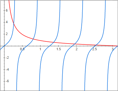
so has no more than zeros (counting with their multiplicities) on . On the other hand, for
the equation is equivalent to the following one
From the plots in Figure 2, one can easily see that this equation has exactly simple roots on the interval , satisfying (5).
Moreover, . Thus, the function has the zeros
Now we turn to the case of nonzero potentials. Using (2), we obtain the relation
Applying the standard argument, based on Rouche’s theorem (see, for example, [27, Theorem 1.1.3]), we arrive at the asymptotic formulas (4) for the eigenvalues of the
problem .
∎
3. Periodic inverse Sturm-Liouville problem
Inverse spectral problems on graphs with cycles usually generalize the periodic inverse problem on a finite interval.
We describe the periodic problem on a loop in this section, because we need it for statement and solution of our partial inverse problem.
Define
Denote by
the zeros of the entire function and put , .
The periodic inverse problem is formulated as follows.
Inverse Problem 1.
Given the functions , and the sequence of signs , construct the potential .
Analogs of Inverse Problem 1 for the case of a regular potential has been studied
in [24, 25] (see also paper [26], where the solution of the periodic problem
has been applied to the inverse problem on a graph). However, the known results can be easily generalized for the case .
Indeed, it is easy to check that
(7)
(8)
Consequently, we have
Hence
(9)
Introduce the norming constants
Using the standard methods (see [27, Lemma 1.1.1]), one can show that
(10)
It is proved in [17], that the spectral data uniquely specify
the potential , and an algorithm for the reconstruction is provied.
Thus, Inverse Problem 1 has a unique solution, which can be found by the following algorithm.
Recover the potential from the spectral data , applying the algorithm from [17].
4. Partial inverse problem
In this section, we give the statement of the studied partial inverse problem, prove the uniqueness theorem and develop a constructive algorithm for its solution.
Fix a , and denote by the set of indices .
Consider the subspectrum .
Here and below we assume that the eigenvalues are numbered with respect to their asymptotics according to Lemma 1.
Note that this numeration is not unique, so a finite number of first eigenvalues in can be chosen arbitrarily.
Impose the following assumptions:
() All the values in are distinct.
() All the values in are positive.
() The functions and do not have common zeros.
Assumption () is used for simplicity, the case of multiple eigenvalues require some tecnical modifications
(see discussion in [10]). Assumption () can be achieved by a shift of the spectrum.
Assumption () is the only principal one. One can easily check, that () is equivalent to the condition
, .
Under assumptions ()–(), we study the following partial inverse problem.
Inverse Problem 2.
Given the potential , the subspectrum and the signs ,
find the potential .
Proceed to the solution of the formulated problem.
Using relations (2), we get
(11)
where and are some real-valued functions from .
Substituting (11) into (3), we derive the relation
(12)
where
(13)
Introduce the real Hilbert space with the scalar product
Obviously, the vector functions
(14)
belong to , and relation (12) can be rewritten in the form
(15)
Lemma 2.
The system of vector functions is complete in .
Proof.
Suppose are such functions, that
(16)
Let for some . By assumption (), we have
. Therefore, using (3), (13) and taking assumption () into account, we get
In the case we have . In view of (3), .
Assumption () yields . Consequently, the relation (16) implies (17). Thus, (17) holds
for all . Hence the entire function
Taking assumption () into account, construct the infinite product
In view of assumption (), the function is entire.
According to the asymptotic formulas (4), the function can be represented in the following form (see [12, Appendix B]):
(20)
where is a nonzero constant. Moreover, one has the following estimate
for some positive and . Together with (19) it yields
By Phragmen-Lindelöf’s and Liouville’s theorems we get . Using (18), one can show that
(as a function of the variable ). However, relation (20) implies
. Hence and .
Recall that are the zeros of . Assumption () requires , .
Consequently, it follows from (18), that
Note that are the eigenvalues of the boundary value problem
therefore , (see [22]).
This asymptotic relation implies that the system
is complete in (see, for example, [23]). Hence . Then we conclude from (19) and , that .
Thus, the system is complete in .
∎
Relying on Lemma 2, we shall prove the uniqueness theorem for the solution of Inverse Problem 2.
Along with the boundary value problem , consider the problem of the same form, but with different potentials
, . We agree that if a certain symbol denotes an object related to , the corresponding symbol
denotes an analogous object related to .
Theorem 1.
Suppose that the boundary value problems and together with their subspectra and
of the form described above satisfy assumptions ()–(), and a.e. on ,
, . Then a.e. on . Thus, Inverse Problem 2
has a unique solution.
Proof.
The relation a.e. on implies ,
. In view of (13), (14) and ,
we have in and for . Since by Lemma 2
the system is complete in , we conclude from (15), that and
a.e. on . Then relation (11) yields , .
In addition, we have , so follows from the uniqueness of the solution
of periodic Inverse Problem 1.
∎
Theorem 2.
The system of vector functions is a Riesz basis in .
Let us show that the system is a Riesz basis in .
It follows from the results of [12, Appendix A], that the systems
and are Riesz bases in .
Consider the linear operator , defined as follows.
where
i.e. are the coordinates of the function with respect to the Riesz basis .
It follows from the Riesz-basis property, that there exist positive constants and such that
Consequently, the operator and its inverse:
are bounded in . Note that the operator transforms the sequence into a Riesz basis
in :
Hence the system is also a Riesz basis.
Since the system is complete by Lemma 2 and
-close to the Riesz basis , we conclude that is a Riesz basis in .
∎
Recovering the vector function from its coordinates with respect to the Riesz basis, one can solve Inverse Problem 2
by the following algorithm.
Algorithm 2.
Let the potential , the eigenvalues and the signs be given.
1.
Construct the functions and .
2.
Find the vector functions and the numbers , using (13) and (14).
3.
Construct the vector function by its coordinates with respect to the Riesz basis (see (15)), i.e. find the functions
and .
Recover the potential from , and , using Algorithm 1.
Acknowledgment.
The author C.-F. Yang was supported in part by the National Natural Science Foundation of
China (11171152, 11611530682 and 91538108) and by the Natural Science Foundation of
the Jiangsu Province of China (BK 20141392).
The author N. P. Bondarenko was supported by the Russian Federation
President Grant MK-686.2017.1, by Grant 1.1660.2017/4.6 of the Russian
Ministry of Education and Science, and by Grants
16-01-00015, 17-51-53180 of the Russian Foundation for Basic Research.
References
[1]
Kuchment, P. Graph models for waves in thin structures, Waves in Random Media 12:4 (2002), R1–R24.
[2]
Analysis on Graphs and Its Applications, edited by P. Exner, J.P. Keating, P. Kuchment,
T. Sunada and Teplyaev, A. Proceedings of Symposia in Pure Mathematics, AMS, 77.
(2008).
[3]
Pokorny, Yu. V.; Penkin, O. M.; Pryadiev, V. L. et al. Differential Equations on Geometrical Graphs,
Fizmatlit, Moscow (2004) (Russian).
[4]
Kuchment, P. Quantum graphs. Some basic structures. Waves Random Media 14 (2004),
S107–S128.
[5]
Yurko, V. A. Inverse spectral problems for differential operators on spatial networks, Russian Mathematical Surveys 71:3 (2016), 539–584.
[6]
Pivovarchik, V. N. Inverse problem for the Sturm-Liouville equation on a simple graph,
SIAM J. Math. Anal. 32:4 (2000), 801–819.
[7]
Yang, C.-F. Inverse spectral problems for the Sturm-Liouville operator on a -star graph,
J. Math. Anal. Appl. 365 (2010), 742–749.
[8]
Yang, C.-F.; Yang X.-P. Uniqueness theorems from partial information of the potential on a
graph, J. Inverse Ill-Posed Prob. 19 (2011), 631- 639.
[9]
Yurko, V. A. Inverse nodal problems for the Sturm-Liouville differential operators on a star-type graph,
Siberian Math. J. 50:2 (2009), 373- 378.
[10]
Bondarenko, N. P. A partial inverse problem for the Sturm Liouville operator on a star-shaped graph,
Anal. Math. Phys. (2017), DOI: 10.1007/s13324-017-0172-x
[11]
Bondarenko, N. P. Partial inverse problems for the Sturm-Liouville operator on a star-shaped graph
with mixed boundary conditions, J. Inverse Ill-Posed Probl. (2017),
published online 2017-03-16, DOI: 10.1515/jiip-2017-0001.
[12]
Bondarenko, N. P. A 2-edge partial inverse problem for the Sturm-Liouville operators with singular potentials on a star-shaped graph,
Tamkang J. Math. (2017, accepted for publication), preprint: arXiv:1702.08293 [math.SP].
[13]
Marchenko, V.; Mochizuki, K.; Trooshin, I. Inverse scattering on a graph containing
circle. Analytic Methods of Analysis and Differ. Equations: AMADE 2006,
237–243. Cambridge Sci. Publ., Cambridge, 2008.
[14]
Mochizuki, K.; Trooshin, I. On the scattering on a loop shaped graph. Evolution
Equations of hyperbolic and Schroedinger type, 227–245, Progr. Math., 301,
Birkhauser/Springer. Basel A6, Basel, 2012.
[15]
Kurasov P. Inverse scattering for lasso graph. J. Math. Phys. 54 (2013), No. 4,
04210314
[16]
Hochstadt, H.; Lieberman, B. An inverse Sturm-Liouville problem with mixed given data, SIAM J. Appl. Math. 34 (1978), 676–680.
[17]
Hryniv, R. O.; Mykytyuk, Ya. V. Inverse spectral problems for Sturm-Liouville operators
with singular potentials, Inverse Problems 19 (2003), 665-684.
[18]
Hryniv, R.O.; Mykytyuk, Ya. V. Inverse spectral problems for Sturm-Liouville operators with singular potentials, II. Reconstruction by two spectra, in: V. Kadets, W. Zelazko (Eds.), Functional Analysis and Its Applications, in: North-Holland Math. Stud., vol. 197, North-Holland Publishing, Amsterdam (2004), 97 114.
[19]
Hryniv, R.O.; Mykytyuk, Ya. V. Half-inverse spectral problems for Sturm-Liouville
operators with singular potentials, Inverse Problems 20 (2004), 1423–1444.
[20]
Hryniv, R. O.; Mykytyuk, Ya. V. Transformation operators for Sturm-Liouville operators with singular
potentials, Math. Phys. Anal. Geom. 7 (2004), 119–149.
[21]
Freiling, G.; Ignatiev, M.; Yurko, V. An inverse spectral problem for Sturm-Liouville operators with singular potentials on star-type graph, Proc. Symp. Pure Math. 77 (2008), 397–408.
[22]
Savchuk, A. M. On the eigenvalues and eigenfunctions of the Sturm-Liouville operator with a singular potential,
Mathematical Notes 69:2 (2001), 245–252.
[23]
He, X.; Volkmer, H. Riesz bases of solutions of Sturm-Liouville equations, J. Fourier Anal. Appl. 7:3 (2001), 297–307.
[24]
Stankevich, I. V. An inverse problem of spectral analysis for Hill’s equations, Doklady Akad. Nauk
SSSR 192, no. 1 (1970), 34–37 (Russian).
[25]
Marchenko, V. A.; Ostrovskii, I. V. A characterization of the spectrum of the Hill operator, Mat.
Sbornik 97 (1975), 540 -606 (Russian); English transl. in Math. USSR Sbornik 26 (1975), 4, 493- 554.
[26]
Yurko, V. A. Inverse problems for Sturm-Liouville operators on graphs with a cycle, Operators and Matrices 2:4 (2008), 543–553.
[27]
Freiling, G.; Yurko, V. Inverse Sturm-Liouville Problems and Their Applications. Huntington,
NY: Nova Science Publishers (2001).
Chuan-Fu Yang
Department of Applied Mathematics, Nanjing University of Sciences and Technology,
Nanjing, 210094, Jiangsu, China,
email: chuanfuyang@njust.edu.cn
Natalia Pavlovna Bondarenko
1. Department of Applied Mathematics, Samara National Research University,
Moskovskoye Shosse 34, Samara 443086, Russia,
2. Department of Mechanics and Mathematics, Saratov State University,
Astrakhanskaya 83, Saratov 410012, Russia,
e-mail: BondarenkoNP@info.sgu.ru