Real-space grid representation of momentum and kinetic energy operators for electronic structure calculations

Abstract

We show that the central finite difference formula for the first and the second derivaxtive of a function can be derived, in the context of quantum mechanics, as matrix elements of the momentum and kinetic energy operators using, as a basis set, the discrete coordinate eigenkets $|x_{n}\rangle$ defined on the uniform grid $x_{n}=na$. Simple closed form expressions of the matrix elements are obtained starting from integrals involving the canonical commutation rule. A detailed analysis of the convergence toward the continuum limit with respect to both the grid spacing and the approximation order is presented. It is shown that the convergence from below of the eigenvalues in electronic structure calculations is an intrinsic feature of the finite difference method.

I Introduction

The last decade has witnessed a growing interest in electronic structure computational schemescol (2015); Beck (2000); Enkovaara et al. (2010); Michaud-Rioux et al. (2016); Hernández et al. (2007) based on the real-space finite difference representation of both the momentum and kinetic energy operators. The main advantage of the method when applied to either the Schrödinger or the DFT Kohn and Sham equationsKohn and Sham (1965), particularly within the pseudopotential density functional theoryChelikowsky et al. (1994), is the highly local structure of the relevant matrices. This feature allows for both a significant reduction of computer memory and for the use of efficient parallel algorithms Burdick et al. (2003) paving the way toward grid-based linear scaling methods. Ab initio electronic structureBeck (2000); Chelikowsky et al. (1994); Fattebert and Bernholc (2000); Castro et al. (2006); Andrade et al. (2015) and molecular dynamics codesSchmid (2004) have successfully been implemented and tested. Moreover, adaptive mesh refinementsModine et al. (1997) and multigrid strategiesBriggs et al. (1996) can be used for gaining local resolution only where it is needed. Finally, it is worth mentioning that the finite difference method is also a very good conceptualDatta (2005) and practicalFujimoto and Hirose (2003); Khomyakov and Brocks (2004) tool for the study of electric current flow in nanodevices.

Other electronic structure computational methods closely related to real space grids are finite elements schemesWhite et al. (1989), discrete variable representationsLiu et al. (2003), Lagrange meshesVarga et al. (2004), nonorthogonal generalized Wannier functionsSkylaris et al. (2005), and waveletsArias (1999); Genovese et al. (2008). All these methods have in common a real space grid whose points are associated to localized basis functionsBaye (2006). As such, it seems that there is not connection between this class of methods and finite differences. We shall show in the following that indeed there is a link when the continuum limit in the finite differences is approached.

For entering the core of the problem discussed here, let us briefly recall how the finite difference method works. The starting point is the choice of the way in which the kinetic energy operator is represented on a discretized space. Let us consider a one dimensional grid (the extension to two and three dimensional Cartesian grids is trivial) made of $N+1$ equally spaced points defined by $x_{n}=na$ with $n=0,1..,N$. The lowest-order approximation to the second derivative is obtained considering only three grid points $x_{n+1},$ $x_{n}$ and $x_{n-1}$. With a Taylor series it is easy to see that the lowest order approximation of second derivative at $x_{n}$ is given by

$$\frac{d^{2}\psi(x_{n})}{dx^{2}}\approx\frac{1}{a^{2}}\left[\psi(x_{n-1})-2\psi(x_{n})+\psi(x_{n+1})\right].$$ (1)

Higher order expressions involving wave function values at $x_{n\pm m}$ can be obtained by means of specific algorithmsFornberg (1998). In general, a finite difference representation of the second derivative takes the form

$$\frac{d^{2}\psi(x_{n})}{dx^{2}}\approx\sum_{m=-M}^{M}C_{m}\psi(x_{n+m}),$$ (2)

where the integer number $M$, which we define as the representation order, controls the accuracy. Whichever method is used for determining the coefficients $C_{m}$, it is clear that the kinetic energy representation induced by Eq. (2) does not apparently have an explicit basis set. In other words, although the $C_{m}$ can formally be viewed as the entries of the kinetic energy matrix, it is not at all clear whether or not there exists an underlying basis set. This is, in our opinion, an interesting and fertile point that has not been discussed in the literature.

A further point is represented by the convergence properties toward the continuous space, that is, the limit of vanishing grid spacing. For instance, practical finite difference DFT electronic structure calculations show that the total energy converges from below with respect to both the grid spacing and the order $M$Beck (2000); Maragakis et al. (2001); Skylaris et al. (2002). It is generally believed that this is an important limitation preventing from developing convergence schemes.

The core of this work is first of all to show that the finite difference method has discrete coordinate eigenkets as the underlying basis set. We obtain this result by explicitly constructing the matrix elements of both the linear momentum and kinetic energy operators. Interestingly, the unique starting point of the derivation is the use of integrals involving the canonical commutations between the operators $\widehat{x}$ and $\widehat{p}$. In a way, we leave to the quantum mechanics rules the determination of the optimal matrix elements. We show that it is possible to obtain simple analytical expressions for the matrix elements so that their convergence towards the continuum limit and the connection with other real space methods can be discussed in detail. The theory is complemented with some explanatory numerical examples.

II The momentum operator

Let us associate to each grid point $x_{n}$ the ket $|x_{n}\rangle$ which we assume to be an eigenket of the position operator $\hat{x}$. This means that

$$\langle x_{m}|\hat{x}|x_{n}\rangle=x_{n}\delta_{m,n}.$$ (3)

Any state defined on this discretized space can be written as

$$\left|\psi\right\rangle=\sum_{n}\phi_{n}\left|x_{n}\right\rangle.$$ (4)

Although it is not strictly necessary for the present discussion, we can notice here that the numbers $\phi_{n}$ in Eq. (4) are the values of the wave function $\psi(x)$ on the grid points $x_{n}$.

A grid representation of the momentum operator is given by

$$\left\langle x_{n}\right|\hat{p}\left|f\right\rangle=-i\hbar\sum_{m=-M}^{M}W_{m}\left\langle x_{n+m}\right.\left|f\right\rangle,$$ (5)

where $\left|f\right\rangle$ is a generic ket. The real numbers $W_{m}$ are the momentum matrix elements. For a given $M$ there are $2M+1$ grid points over which the $W_{m}$ are different from zero. This means that the set of $W_{m}$ depends on $M$. For indicating explicitly this dependence, we write, from now on, $W_{m}^{(M)}$ and call $M$ the representation order. Taking $\left|f\right\rangle=\left|x_{l}\right\rangle$, from Eq. (5) we have

$$\left\langle x_{n}\right|\hat{p}\left|x_{l}\right\rangle=-i\hbar\sum_{m=-M}^{M}W_{m}^{(M)}\delta_{n+m,l}=-i\hbar W_{l-n}^{(M)},$$ (6)

where $-M\leq l-n\leq M$. Since we want an Hermitian matrix representing $\hat{p}$, we must require

$$W_{-m}^{(M)}=-W_{m}^{(M)},$$ (7)

and this implies that $W_{0}^{(M)}=0$. Additional conditions necessary for determining $W_{m}^{(M)}$ can be derived starting from integrals involving the canonical commutation

$$\left[\hat{x},\hat{p}\right]=i\hbar\hat{I}.$$ (8)

With continuum position eigenkets it is known that

$$\int\left\langle x^{\prime}\right|\left[\hat{x},\hat{p}\right]\left|x^{\prime\prime}\right\rangle dx^{\prime\prime}=i\hbar.$$ (9)

The discrete analog of Eq. (9) is obtained by calculating the matrix elements $\langle x_{n}|\left[\hat{x},\hat{p}\right]|x_{n+m}\rangle$ and summing on $m$. Using Eq. (6) we have

$$\sum_{m=-M}^{M}\left\langle x_{n}\right|\left[\hat{x},\hat{p}\right]\left|x_{n+m}\right\rangle=i\hbar a\sum_{m=-M}^{M}mW_{m}^{(M)}.$$ (10)

It follows that if we want that Eq. (10) gives exactly the same result as Eq. (9), the matrix elements $W_{m}^{(M)}$ must satisfy the equation

$$\sum_{m=1}^{M}mW_{m}^{(M)}=\frac{1}{2a},$$ (11)

where we have used Eq. (7) for limiting the sum to positive $m$. Equation (11) is just enough for determining $W_{m}^{(M)}$ with $M=1$. Indeed, one immediately gets $W_{\pm 1}^{(1)}=\pm 1/2a$ which are exactly the central difference weights for the lowest order first derivative. This an interesting intermediate result. However, the issue now is to show how the most general case of $M>1$ can be handled, that is, how we can generate the necessary additional equations. Since multiple commutators of the type $\left[\hat{x},\left[\hat{x},\ldots,\left[\hat{x},\hat{p}\right]\right]\right]$ are all zero, we have

$$\int\left\langle x^{\prime}\right|\left[\hat{x},\left[\hat{x},\ldots,\left[\hat{x},\hat{p}\right]\right]\right]\left|x^{\prime\prime}\right\rangle dx^{\prime\prime}=0.$$ (12)

In analogy with Eqs. (9) and (10), the discretization of this equation leads us to

$$\sum_{m=-M}^{M}\left\langle x_{n}\right|\left[\hat{x},\left[\hat{x},\ldots,\left[\hat{x},\hat{p}\right]\right]\right]\left|x_{n+m}\right\rangle=\sum_{m=-M}^{M}m^{s}W_{m}^{(M)}=0$$ (13)

where $s$ is the number of times $\hat{x}$ appears in the multiple commutator. Using Eq. (7) it is easy to see that Eq. (13) is identically satisfied when $s$ is even. We are therefore left with

$$\sum_{m=1}^{M}m^{2l+1}W_{m}^{(M)}=0\text{ where }l=1,\ldots M-1.$$ (14)

For a given $M$, the set of Eqs. (14) and (11) can be solved. The final result is

$$W_{m}^{(M)}=\frac{1}{2am\Omega(M,m)},$$ (15)

where we have defined

$$\Omega(M,m)=\prod\limits_{\begin{subarray}{c}l=1\\ l\neq m\end{subarray}}^{M}\left[1-\left(\frac{m}{l}\right)^{2}\right].$$ (16)

The momentum matrix elements are

$$\left\langle x_{n}\right|\hat{p}\left|x_{n+m}\right\rangle=\left\{\begin{array}[c]{ll}0&\text{if }m=0\\ \displaystyle{\frac{-i\hbar}{2am\Omega\left(M,m\right)}}&\text{if }m\neq 0\end{array}\right.$$ (17)

The numerical values of Eq. (17) are identical to those obtained for the first derivative central finite difference weights using the algorithm discussed in Ref.Fornberg (1998). It is useful for the following to calculate the limit of Eq. (16) when $M\rightarrow\infty$. The result is extraordinarily simple

$$\Omega(\infty,m)=\frac{\left(-1\right)^{m+1}}{2},$$ (18)

from which we immediately have

$$\left\langle x_{n}\right|\hat{p}\left|x_{n+m}\right\rangle=\left\{\begin{array}[c]{ll}0&\text{if }m=0\\ \displaystyle{\frac{i\hbar(-1)^{m}}{am}}&\text{if }m\neq 0\end{array}\right.$$ (19)

The actual meaning and implications of this result will be discussed in the next section.

Before closing this section, it may be useful to summarize the main points. The quantum mechanical ’rules’ expressed in Eq. (9) and (12) have guided us to the simple closed form expression (15) of the weights $W_{m}^{(M)}$. Since our derivation has been built on the basis set $|x_{n}\rangle$, we have indirectly proved that this is the basis set of the finite difference scheme.

III The kinetic energy operator

We now derive an expression for the kinetic energy matrix elements following steps that are similar to what we have done for the linear momentum. The kinetic energy can be defined as

$$\left\langle x_{n}\right|\hat{T}\left|f\right\rangle=-\frac{\hbar^{2}}{2\mu}\sum_{\begin{subarray}{c}l=-M\\ l\neq 0\end{subarray}}^{M}C_{l}^{(M)}\left(\left\langle x_{n+l}\right.\left|f\right\rangle-\left\langle x_{n}\right.\left|f\right\rangle\right).$$ (20)

From Eq. (20) and the orthogonality of the set $|x_{n}\rangle$ it is easy to see that

$$\langle x_{n}|\hat{T}|x_{n+m}\rangle=\frac{\hbar^{2}}{2\mu}\left\{\begin{array}[c]{ll}-C_{m}^{(M)}&\text{ if }m\neq 0\vspace{0.2cm}\\ \sum\limits_{\begin{subarray}{c}l=-M\\ l\neq 0\end{subarray}}^{M}C_{l}^{(M)}&\text{ if }m=0\end{array}\right.$$ (21)

The coefficients $C_{m}^{(M)}$ in Eq. (21) can be related to $W_{m}^{(M)}$ taking the matrix elements of $\hat{p}=\frac{\mu}{i\hbar}\left[\hat{x},\hat{T}\right]$ on the basis $|x_{n}\rangle$. The final result is

$$C_{m}^{(M)}=\frac{2W_{m}^{(M)}}{am}.$$ (22)

Inserting Eq. (22) into Eq. (21) we finally have

$$\left\langle x_{n}\right|\hat{T}\left|x_{n+m}\right\rangle=\frac{\hbar^{2}}{2\mu a^{2}}\left\{\begin{array}[c]{ll}\displaystyle{\frac{-1}{m^{2}\Omega(M,m)}}&\text{ if }m\neq 0\vspace{0.2cm}\\ \displaystyle{\sum_{l=1}^{M}\frac{2}{l^{2}\Omega(M,l)}}&\text{ if }m=0\end{array}\right.$$ (23)

Eq. (23) gives a closed form expression for the kinetic energy valid to all orders $M$. The advantage of having an analytical expression of the matrix elements is not only the simplicity with which they can be generated in an electronic structure computer code, but also the possibility of easily looking at their behavior when the representation order $M$ is very large. Indeed, from Eq. (18) it is easy to see that when $M\rightarrow\infty$ Eq. (23) becomes

$$\left\langle x_{n}\right|\hat{T}\left|x_{n+m}\right\rangle=\frac{\hbar^{2}}{2\mu a^{2}}\left\{\begin{array}[c]{ll}\displaystyle{\frac{2(-1)^{m}}{m^{2}}}&\text{ if }m\neq 0\vspace{0.2cm}\\ \displaystyle{\frac{\pi^{2}}{3}}&\text{ if }m=0\end{array}\right.$$ (24)

It should be noted that although Eq. (24) is strictly valid only for a grid made of an infinite number of points, it is nevertheless an interesting results because it establishes a connection between finite difference and pseudospectral methodsJordan and Mazziotti (2004); Baye (2006). It is worth recalling that in a pseudospectral method the wave function is written asBaye (2006)

$$\psi(x)=\sum_{n}a_{n}C_{n}(x),$$ (25)

where the basis $C_{n}(x)$ has the cardinal property

$$C_{n}(x_{m})=\delta_{m,n}.$$ (26)

Because of this property, Eq. (25) becomes

$$\psi(x)=\sum_{n}\psi(x_{n})C_{n}(x).$$ (27)

Although there is a similarity between Eqs. (27) and (4), it should be observed that while in the former the basis and the wave function are defined in a continuous space, in the latter they are defined only on the grid points. In a way we can say that Eq. (27) is the continuum space extension of Eq. (4).

Let us now calculate the matrix elements of the kinetic energy operator $\hat{T}=-\frac{\hbar^{2}}{2\mu}\frac{d^{2}}{dx^{2}}$ on the $sinc$ (also known as Whittaker cardinal) functions

$$sinc(x-x_{n})=\frac{sin\left(\pi(x-x_{n})/a\right)}{\pi(x-x_{n})/a}.$$ (28)

It is quite interesting that the result of this calculationJordan and Mazziotti (2004); Baye (2006) is exactly Eq. (24). In a similar way, it is possible to show that the momentum matrix elements between $sinc$ functions are given by Eq. (19). We therefore see that the connection between the finite difference and the pseudospectral methods goes through the infinite order limit $M\rightarrow\infty$.

IV The convergence towards the continuous space

For having more insights on the convergence properties with respect to $M$ it is necessary to give a sense to the limit $M\rightarrow\infty$ on a space grid made of a finite number of points. As it is well known in solid state theory, an effective way of constructing an infinite lattice out of a finite one is that of taking periodic replicas. We can use exactly the same idea by taking periodic replicas of a grid of length $L=Na$. In this way the limit $M\rightarrow\infty$ has a precise meaning.

On a replicated grid we need to impose periodic boundary conditions. We shall see in a moment that this choice is particularly useful because it allows the analytical calculation of both the momentum and the kinetic energy eigenvalues. Let us show this for the momentum matrix. The eigenvalue equation is

$$\sum_{m=-M}^{M}\langle x_{n}|\hat{p}|x_{n+m}\rangle\left\langle x_{n+m}\right.\left|k\right\rangle=p\left\langle x_{n}\right.\left|k\right\rangle,$$ (29)

where we have indicated with $\langle x_{n}|k\rangle$ the momentum eigenvectors on the grid. It is a simple matter to verify that Eq. (29) can be solved with

$$\left\langle x_{n}\right.\left|k\right\rangle=e^{-ikx_{n}}.$$ (30)

The wave vector $k$ is selected imposing the periodic boundary condition $\left\langle x_{n+N}\right.\left|k\right\rangle=\left\langle x_{n}\right.\left|k\right\rangle$ giving the well known result

$$k_{\nu}=\frac{2\pi\nu}{L}\text{ with }\nu=0,1,2\ldots N-1$$ (31)

where $L=Na$ is the grid length. Inserting Eq. (30) into Eq. (29) and using Eq. (15) we have the eigenvalues

$$p_{\nu}=\frac{\hbar}{a}\sum_{m=1}^{M}\frac{\sin\left(x_{m}k_{\nu}\right)}{m\Omega(M,m)}.$$ (32)

The simple structure of Eq. (32) allows us to study in detail the convergence towards the continuum with respect to both the representation order $M$ and the grid spacing $a$.

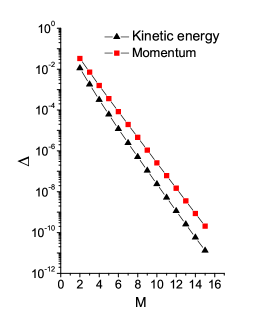
Figure 1: (Color online) The correction $\Delta$ as defined in Eq. (36) for the momentum and Eq. (39) for the kinetic energy as a function of $M$.

However, before doing that, let us also see what we obtain for the kinetic energy. From an eigenvalue equation similar to Eq. (29) we get

$$\varepsilon_{\nu}=\frac{\hbar^{2}}{2\mu a^{2}}\sum_{m=1}^{M}\frac{4}{m^{2}\Omega(M,m)}\sin^{2}\left(\frac{x_{m}k_{\nu}}{2}\right).$$ (33)

We are now ready to take the limit $M\rightarrow\infty$. For the momentum we must use Eqs. (32) and (18). The result is

$$p_{\nu}=\frac{\hbar}{a}\sum_{m=1}^{\infty}\frac{2\left(-1\right)^{m+1}}{m}\sin\left(x_{m}k_{\nu}\right)=\hbar k_{\nu}.$$ (34)

This is quite interesting: it tell us that with a fixed grid spacing $a$, the linear momentum gets exactly the values one would expect for a free particle on a lattice of length $L=Na$ with periodic boundary conditions. The type of convergence behind Eq. (34) can be better appreciated by computing the power series of Eq. (32) with respect to the grid spacing $a$. A lengthy calculation in which we retain, for each order $M$, the first non vanishing terms gives

$$p_{\nu}=\hbar k_{\nu}\left[1-\left(k_{\nu}a\right)^{2M}\Delta_{p}(M)+\ldots\right]$$ (35)

where

$$\Delta_{p}(M)=\frac{2(M+1)}{\left(2M+2\right)!}\left|\sum_{m=1}^{M}\frac{m^{2M}}{\Omega(M,m)}\right|.$$ (36)

It should be noted that since $\Delta_{p}(M)$ is always positive, Eq. (35) shows that the convergence to the exact momentum is from below.

The limit $M\rightarrow\infty$ for the kinetic energy is easily obtained from Eqs. (33) and (18). The result is

$$\varepsilon_{\nu}=\frac{\hbar^{2}}{2\mu a^{2}}\sum_{m=1}^{\infty}\frac{4\left(-1\right)^{m+1}}{m^{2}}\sin^{2}\left(x_{m}k_{\nu}\right)=\frac{\hbar^{2}k_{\nu}^{2}}{2\mu}.$$ (37)

Again, we get the exact kinetic energy of a free particle on a lattice with periodic boundary conditions.. In analogy with Eq. (35), a power series of Eq. (33) leads to

$$\varepsilon_{\nu}=\frac{\hbar^{2}k_{\nu}^{2}}{2\mu}\left[1-\left(k_{\nu}a\right)^{2M}\Delta_{\varepsilon}(M)\ldots\right],$$ (38)

where we have defined

$$\Delta_{\epsilon}(M)=\frac{2}{\left(2M+2\right)!}\left|\sum_{m=1}^{M}\frac{m^{2M}}{\Omega(M,m)}\right|.$$ (39)

The same conclusions we have drawn for the momentum hold in this case. In particular, it is worth stressing the convergence from below which plays an important role in electronic structure calculations.

To give a hint on how small the the relative error $\Delta$ are, we show in Fig. 1 a plot of Eqs. (36) and (39) as a function of $M$. It can be seen from this figure that $\Delta$ quickly goes down so that one would expect that in a practical numerical calculation there should be no need of using values of $M$ larger than about $6\div 8$. This is important because keeping a banded kinetic energy matrix is a prerequisite for a fast calculation.

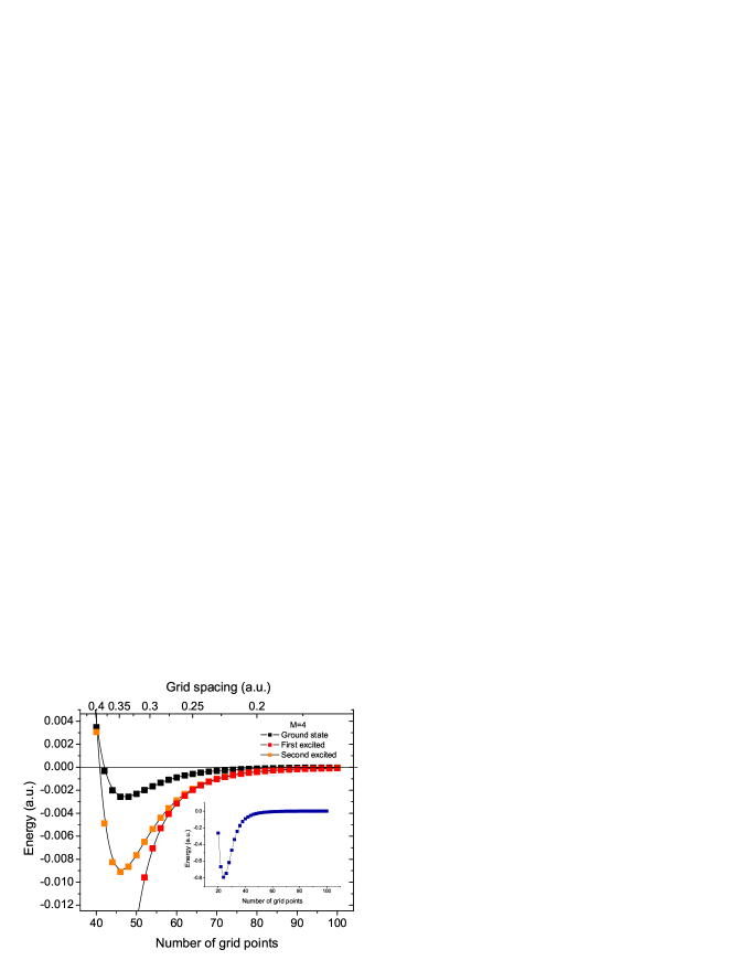
Figure 2: (Color online) Convergence of the eigenvalues of the one dimensional Schrödinger equation discussed in the text versus the number of grid points. The inset shows the eigenvalues sum.

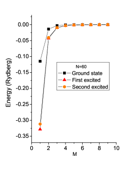
Figure 3: (Color online) Convergence of the eigenvalues of the one dimensional Schrödinger equation discussed in the text versus the representation order $M$.

Figure 4: (Color online) Convergence of the total energy of a C₂ molecule versus the representation order $M$ with a grid spacing $a=0.32$ atomic units.

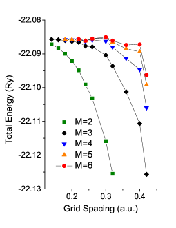
Figure 5: (Color online) Convergence of the total energy of a C₂ molecule versus the grid spacing for different values of the representation order $M$.

V Numerical examples

The convergence properties discussed in the previous section are here verified on two very different numerical examples. The first one is the one dimensional Schrödinger equation with the potential $V(x)=-U_{0}/cosh^{2}(\alpha x)$ for which an exact analytical solution is availableLandau (1976). Choosing $U_{0}=-21.0Ry$ and $\alpha=1.4$, it can be seen that the bound states are just three.

Using the kinetic energy matrix elements of Eq. (23), we have numerically calculated the three eigenvalues changing both $M$ and $N$. The convergence towards the exact eigenvalues on changing $N$ is shown in Fig. 2 while that obtained on changing $M$ is shown in Fig. 3. Moreover, in the inset of Fig. 2 we also show the convergence of the eigenvalues sum. The data in Fig. 2 show that a monotonic convergence from below is recovered only for sufficiently large $N$. On the contrary, as shown in Fig. 3, the convergence with respect to $M$ is fully monotonic. The difference is due to the way the potential contributes to the final result. In Fig. 2 we change the grid spacing so that the potential is sampled differently for each $N$ whereas in Fig. 3 we are only changing the representation order in the kinetic energy matrix. The convergence from below shown in Fig. 3 is consistent with the data of Fig. 1.

The second numerical example we have analyzed is that of a DFT calculation of the ground state of a C₂ molecule. The calculations have been performed using the finite difference pseudopotential method developed by Chelikowsky et alChelikowsky et al. (1994). In Fig.4 we show the convergence of the total energies with respect to the representation order $M$ while in Fig.5 we show the convergence versus the grid spacing. In both the cases the convergence from below due to the kinetic energy is quite evident. Despite the enormous difference in the computational complexity with respect to the one dimensional case, the general trends are similar.

A last example is here reported to evaluate, in bulk silicon, the convergence properties of the total energy with respect to the grid spacing and the representation order. We used Octopus scientific code to perform DFT real space calculationsCastro et al. (2006).

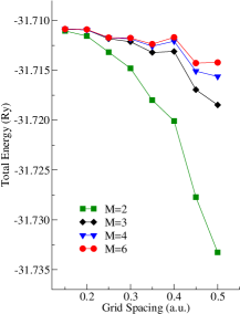
Figure 6: (Color online) Convergence of the total energy of bulk silicon versus the grid spacing, for several values of the representation order.

A 2x2x2 Monkhorst Pack grid was adopted to perform integrations over the first Brillouin zone, together with a Perdew-Zunger LDA exchange-correlation functional, and a 8-atom cubic conventional cell, with a lattice constant fixed at $10.3$ a.u. The total energy was evaluated on changing the representation order and the grid spacing, each time redoing the selfconsistent procedure. The convergence of the total energy with respect to the grid spacing, for several values of $M$, is reported in figure 6. The scaling is qualitatively similar to the example illustrated in the previous section, and the results discussed above are confirmed. Even in this case, the convergence is from below. The total energy is fully monotonic with respect to the representation order (at fixed grid spacing), and shows a striking similarity to figure 4 (for this reason the graph is not reported here). Instead, as reported in figure 6, the convergence is always from below, but with oscillating features, when the grid spacing decreases at a fixed value of $M$. It is worth noticing that a higher representation order leads to a faster convergence with respect to the grid spacing. A tradeoff, in terms of computational time, has to be found between representation order and grid spacing. However, the use of a high value of $M$ is surely convenient. The default value chosen by the code for the representation order is $M=4$.

VI Conclusions

With this work we have made an attempt of resolving two main misconceptions related to finite difference electronic structure calculations. The first is that it is not really true that a finite difference representation has not a basis set and the second is that the anti variational behavior is not a limitation of the method.

The proof that a basis set does exist has been a constructive one in the sense that we have derived explicit expressions for the momentum and kinetic energy matrix elements showing that they are identical to the central finite difference weights of the first and second derivatives.

The convergence from below has been fully characterized calculating the momentum and kinetic energy eigenvalues using periodic boundary conditions. We have derived for both the operators two formulas, Eqs. (36) and (39), that we think can be useful for developing convergence criteria. We hope to have made clear that the anti variational behavior is an intrinsic feature of finite difference method intimately connected to the fact for each couple of the integer number $N$ and $M$ one has a different representation of the operators.

An important point of this work is that the continuum momentum and kinetic energies can be obtained with two different limits. The first one is obtained taking the limit of large values of $M$, the representation order, with a fixed grid spacing. This limit, taken on a finite grid, has a meaning only when periodic boundary conditions are imposed. The exact linear momentum and kinetic energy of a free particle on a lattice are recovered. The second limit consists in sending the grid spacing to zero while keeping $M$ unchanged. We have shown that also in this case the continuum momentum and kinetic energy are recovered.

A concluding remark may be that the above result may be useful for reviewing, from a different perspective, the quantum mechanics in a discretized space.

References

- col (2015) Themed collection: Real space numerical grid methods in quantum chemistry, Phys. Chem. Chem. Phys. 2015, 17.
- Beck (2000) Beck, T. L. Rev. Mod. Phys. 2000, 72, 1041–1080.
- Enkovaara et al. (2010) Enkovaara et al. Journal of Physics: Condensed Matter 2010, 22, 253202.
- Michaud-Rioux et al. (2016) Michaud-Rioux, V.; Zhang, L.; Guo, H. Journal of Computational Physics 2016, 307, 593 – 613.
- Hernández et al. (2007) Hernández, E. R.; Janecek, S.; Kaczmarski, M.; Krotscheck, E. Phys. Rev. B 2007, 75, 075108.
- Kohn and Sham (1965) Kohn, W.; Sham, L. J. Phys. Rev. 1965, 140, A1133–A1138.
- Chelikowsky et al. (1994) Chelikowsky, J. R.; Troullier, N.; Saad, Y. Phys. Rev. Lett. 1994, 72, 1240–1243.
- Burdick et al. (2003) Burdick, W.; Saad, Y.; Kronik, L.; Vasiliev, I.; Jain, M.; Chelikowsky, J. Comput. Phys. Commun. 2003, 156, 22–42.
- Fattebert and Bernholc (2000) Fattebert, J.-L.; Bernholc, J. Phys. Rev. B 2000, 62, 1713–1722.
- Castro et al. (2006) Castro, A.; Appel, H.; Oliveira, M.; Rozzi, C. A.; Andrade, X.; Lorenzen, F.; Marques, M. A. L.; Gross, E. K. U.; Rubio, A. Phys. Status Solidi B 2006, 243, 2465–2488.
- Andrade et al. (2015) Andrade et al. Phys. Chem. Chem. Phys. 2015, 17, 31371–31396.
- Schmid (2004) Schmid, R. J. Comput. Chem 2004, 25, 799.
- Modine et al. (1997) Modine, N. A.; Zumbach, G.; Kaxiras, E. Phys. Rev. B 1997, 55, 10289–10301.
- Briggs et al. (1996) Briggs, E. L.; Sullivan, D. J.; Bernholc, J. Phys. Rev. B 1996, 54, 14362–14375.
- Datta (2005) Datta, S. Quantum transport atom to transistor; Cambridge University Press: Cambridge, UK, 2005.
- Fujimoto and Hirose (2003) Fujimoto, Y.; Hirose, K. Phys. Rev. B 2003, 67, 195315.
- Khomyakov and Brocks (2004) Khomyakov, P. A.; Brocks, G. Phys. Rev. B 2004, 70, 195402.
- White et al. (1989) White, S. R.; Wilkins, J. W.; Teter, M. P. Phys. Rev. B 1989, 39, 5819–5833.
- Liu et al. (2003) Liu, Y.; Yarne, D. A.; Tuckerman, M. E. Phys. Rev. B 2003, 68, 125110.
- Varga et al. (2004) Varga, K.; Zhang, Z.; Pantelides, S. T. Phys. Rev. Lett. 2004, 93, 176403.
- Skylaris et al. (2005) Skylaris, C.-K.; Haynes, P. D.; Mostofi, A. A.; Payne, M. C. J. Chem. Phys. 2005, 122, 084119.
- Arias (1999) Arias, T. A. Rev. Mod. Phys. 1999, 71, 267–311.
- Genovese et al. (2008) Genovese, L.; Neelov, A.; Goedecker, S.; Deutsch, T.; Ghasemi, S. A.; Willand, A.; Caliste, D.; Zilberberg, O.; Rayson, M.; Bergman, A.; Schneider, R. J. Chem. Phys. 2008, 129, 014109.
- Baye (2006) Baye, D. Phys. Status Solidi B 2006, 243, 1095–1109.
- Fornberg (1998) Fornberg, B. SIAM Rev. 1998, 40, 685–691.
- Maragakis et al. (2001) Maragakis, P.; Soler, J.; Kaxiras, E. Phys. Rev. B 2001, 64, 193101.
- Skylaris et al. (2002) Skylaris, C.-K.; Diéguez, O.; Haynes, P. D.; Payne, M. C. Phys. Rev. B 2002, 66, 073103.
- Jordan and Mazziotti (2004) Jordan, D. K.; Mazziotti, D. A. J. Chem. Phys. 2004, 120, 574.
- Landau (1976) Landau, L. D. Quantum Mechanics; Pergamon Press, Oxford, 1976.