CP violations in a predictive $A_{4}$ symmetry model

Abstract

We will investigate numerically a seesaw model with $A_{4}$ flavor symmetry to find allowed regions satisfying the current experimental neutrino oscillation data, then use them to predict physical consequences. Namely, the lightest active neutrino mass is of the order of $\mathcal{O}(10^{-2})$ eV. The effective neutrino mass $|\langle m\rangle|$ associated with neutrinoless double beta decay is in the range $[0.002\;\mathrm{eV},0.038\;\mathrm{eV}]$ and $[0.048\;\mathrm{eV},0.058\;\mathrm{eV}]$, corresponding to the normal and the inverted hierarchy schemes, respectively. Other relations among relevant physical quantities are shown, so that they can be determined if some of them are confirmed experimentally. The recent data of the baryon asymmetry of the Universe ($\eta_{B}$) can be explained via leptogenesis caused by the effect of the renormalization group evolution on the Dirac Yukawa couplings, provided the right-handed neutrino mass scale $M_{0}$ ranges from $\mathcal{O}(10^{8})$ GeV to $\mathcal{O}(10^{12})$ GeV for $\tan\beta=3$. This allowed $M_{0}$ range is different from the scale of $\mathcal{O}(10^{13})$ GeV for other effects that also generate a consistent $\eta_{B}$ from leptogenesis. The branching ratio of the decay $\mu\rightarrow\,e\gamma$ may reach future experimental sensitivity for very light values of $M_{0}$. Hence, it will be inconsistent with the $M_{0}$ range predicted from the $\eta_{B}$ data whenever this decay is detected experimentally.

I Introduction

The experimental data for neutrino oscillation definitely affirmed that neutrinos are massive and they are mixing. Based on neutrino experimental data, in 2002, P. F. Harrison et al. Harrison:2002er ; Harrison:2002kp ; Harrison:2002et ; Harrison:2003aw proposed the structure of neutrino mixing matrix named tri-bimaximal (TB). According to this structure, the reactor mixing angle, $\theta_{13}$, is zero and the Dirac CP-violating phase has no meaning. Subsequently, there was a lot of effort to build simple models leading to the TB mixing pattern of leptons. An interesting way seems to be the use of some discrete non-Abelian flavor groups added to the gauge group of the Standard Model (SM). There is a series of such models based on the symmetry groups $A_{4}$ Ma:2001dn ; Babu:2002dz ; Altarelli:2005yp ; Altarelli:2005yx ; Bazzocchi:2007na ; Brahmachari:2008fn ; Adhikary:2008au , $T^{\prime}$ Feruglio:2007uu ; Chen:2007afa ; Frampton:2007et ; Frampton:2009fw , and $S_{4}$ Pakvasa:1978tx ; Brown:1984mq ; Lee:1994qx ; Ma:2005pd . These models are usually realized at some high-energy scale $\Lambda$ and the groups are spontaneously broken due to a set of scalar multiplets. On the other hand, the most up-to-date data from neutrino oscillation experiments shows that the reactor mixing angle is relatively large, $\theta_{13}\sim 8^{\textrm{o}}$ Tanabashi:2018oca . As a result, the models mentioned have been improved in order to generate a non-zero value of $\theta_{13}$ as well as leptogenesis; see, for example the models with $A_{4}$ symmetry given in Refs. Altarelli:2005yx ; Altarelli:2012ss ; Ma:2012xp ; Chen:2012st ; Ahn:2013mva , where higher-order corrections to fermion mass matrices were considered. However, according to these works, just the inclusion of higher-order corrections would not produce such a large value of $\theta_{13}$ consistent with experiment. Improved models with modular $A_{4}$ symmetry groups have also been constructed recently to explain the neutrino oscillation data Novichkov:2018yse ; Ding:2019zxk . On the other side, several models were built by adding new sources of $A_{4}$ breaking at the leading orders into the original $A_{4}$ models Altarelli:2005yx , so that they can esuccessfully xplain both experimental values of $\theta_{13}$ and leptogenesis; see, for example, Refs. Adhikary:2008au ; Karmakar:2015jza ; Chen:2012st ; Morisi:2013qna ; Karmakar:2014dva , and a list of other models reviewed in Ref. Barry:2010zk . In particular, a soft breaking $A_{4}$ term was introduced in Ref. Adhikary:2008au , three singlet flavons were used in Refs. Karmakar:2015jza ; Chen:2012st , and two singlet flavons $\xi,\xi^{\prime}$ transform as $1,1^{\prime}$ of the $A_{4}$ in Refs. Chen:2012st ; Morisi:2013qna ; Karmakar:2014dva in order to accommodate with the present neutrino data. However, leptogenesis was not studied in Ref. Morisi:2013qna , while in Ref. Karmakar:2014dva , to explain conventional leptogenesis the authors considered the contribution of the next-to-leading order (NLO) corrections to the right-handed neutrino (RHN) mass matrix in the suppersymmetry framework. Namely, two new NLO terms corresponding to two new independent parameters were introduced by hand, then their allowed values were investigated to guarantee successful leptogenesis, leading to a prediction that the RHN mass scale is around $\mathcal{O}(10^{13})$ GeV. But these terms will not survive in other models where new charge assignments of discrete symmetries are chosen to cancel them. In addition, it seems that this approach still needs more independent parameters than an alternative presented in Ref. Adhikary:2008au , where a single softly broken $A_{4}$ term was added into the original model to successfully solve both neutrino data and leptogenesis, leading to a prediction of the RHN mass scale of $O(10^{13})$ GeV. The model mentioned in Ref. Adhikary:2008au is the simplest extension of the original one discussed in Ref. Altarelli:2005yx .

In this work we will study another simple approach, based on the model introduced in Ref. Karmakar:2014dva , but only effects of renormalization group (RG) evolution of the Dirac Yukawa coupling matrix will be included to study flavored leptogenesis. Because only two flavon singlets are added into the model, and the NLO terms like those mentioned in Ref. Karmakar:2014dva are excluded by the total symmetry, only one new term appears in the model, therefore it is also as simple as the model given in Ref. Adhikary:2008au . We believe that the effect caused by just the RG is as important as the effects arising from the NLO terms mentioned in Ref. Karmakar:2014dva , where successful leptogenegis requires a large RHN mass scale of around $\mathcal{O}(10^{13})$ GeV. Also, the same RHN mass scale is needed for successful leptogenesis in the model constructed in Ref. Adhikary:2008au . This scale is only three orders less than the perturbative limit of the seesaw (SS) model Minkowski:1977sc ; Mohapatra:1979ia ; GellMann:1980vs ; Yanagida:1979as ; Schechter:1980gr $\sqrt{4\pi}\times 174/10^{-12}\sim\mathcal{O}(10^{16})$. Our work will find an interesting answer for the question of whether the RG effects need a lower RHN mass scale to explain leptogenesis, or whether they have the same order of $10^{13}$ GeV predicted previously. Anyway, we can discuss which effects are dominant or whether there any properties to distinguish these two effects if they appear simultaneously in the same RHN mass scale. The correlation of the two effects will also be very interesting, but we will leave this for further study.

Besides generating a tiny neutrino mass, the seesaw model has another physics consequence called leptogenesis for the generation of the observed baryon asymmetry of the Universe (BAU) by the charge/parity (CP) asymmetric decay of heavy RHNs Fukugita:1986hr ; Giudice:2003jh ; Buchmuller:2004nz . If the BAU was generated by leptogenesis, then CP-violation in the lepton sector must exist. For Majorana neutrinos, there are one Dirac and two Majorana CP violating phases. One of the phases (or a combination of them) in principle can be measured by neutrinoless double beta ($0\nu 2\beta$) decay Bilenky:2001rz ; Pascoli:2001by ; Pascoli:2002qm ; Petcov:2004wz experiments. Also, the TB mixing structure forbids low-energy CP violation in neutrino oscillation, due to $U_{e3}=0$, and also forbids high-energy CP violation in leptogenesis. Therefore, any observations of leptonic CP violation, for instance in $0\nu 2\beta$ decay, can strengthen our believe in leptogenesis by demonstrating that CP is not a lepton symmetry.

In this work we consider an expansion of the SM by the seesaw realization of an $A_{4}$ discrete symmetric model and its phenomena. Apart from two SM scalar doublets taking responsibility for spontaneously breaking of $A_{4}$ and the SM gauge groups, this model contains additional $SU(2)_{L}$ scalar singlets, namely two singlets $\xi^{\prime},\xi^{\prime\prime}$ transform as $1^{\prime},1^{\prime\prime}$ and two triplets of the $A_{4}$. If the RHN mass matrix’s components resulting from the contributions of the vacuum expectation values (VEVs) of two scalar singlets (of both $SU(2)_{L}$ and $A_{4}$) are exactly the same, then the model generates the TB pattern of lepton mixing matrix and hence leptogenesis does not work. We therefore study the case where those components are independent, and we find the allowed regions of the parameter space of the model that satisfy the low-energy data and the recent BAU data through flavored leptogenesis that arise from the RG effects at a high scale of RHN masses. At low-energy, although our model inherits similar properties in the lepton sector to some previous works Karmakar:2014dva , where some of the unknown parameters were fixed to determine the allowed regions, in this work we will scan the whole parameter space to collect all possible allowed regions satisfying the recent neutrino oscillation data. Based on this, we give interesting physical consequences of $|\langle m\rangle|$ and lepton flavor violating (LFV) decays. We will also determine the RHN mass scale at high energy that successfully explains the BAU data originating from just the RG effect. The allowed range of RHN mass scale will be used to compare with those concerned previously, which come from other sources of soft breaking $A_{4}$ or NLO terms that are forbidden in our model.

This work is organized as follows. In Sect. II we summarize all the ingredients for constructing the $A_{4}$ model with the seesaw mechanism, focusing on the Higgs and lepton sectors. After that, we present, step by step, our approach to numerically investigating the parameter space of the model to guarantee that all allowed regions satisfying the recent neutrino oscillation data are pointed out. Following this, we continue predicting some consequences related to the low-energy phenomena of the lepton sector. Section III is devoted to studying the leptogenesis originating purely from the RG effects, where the allowed range of the RHN mass scale that satisfies the BAU data will be determined. Section IV will pay attention to the LFV decay of charged leptons, and will show that these decays can be considered as another indirect channel to estimate the RHN mass scale. Important conclusions from our work are given in the last section, section V. In addition, there are three appendices to add more detailed discussions on the $A_{4}$ rules, the Higgs potential, and analytic formulas for one-loop contributions to the LFV decays in the unitary gauge.

II The $A_{4}$ symmetry model with seesaw mechanism

The non-Abelian $A_{4}$ is a group of even permutations of four objects and has $4!/2=12$ elements. All the properties of this group needed for model construction were given in Ref. Altarelli:2005yx . This paper will work in the $A_{4}$ basis introduced by G. Altarelli and F. Feruglio, as reviewed in Appendix A. In this work we promote the $A_{4}$ proposed in Refs. Adhikary:2008au ; Karmakar:2014dva with two Higgs singlets to accompany the seesaw mechanism. The model contains several $SU(2)_{L}\otimes U(1)_{Y}$ Higgs singlets, where two of them ($\xi^{\prime},\ \xi^{\prime\prime}$) are $A_{4}$ singlets, while the remaining ($\phi_{S},\ \phi_{T}$) are triplets. The SM lepton doublets are assigned to be three components of one $A_{4}$ triplet, while three right-handed charged leptons $e_{R},\mu_{R},\tau_{R}$ are assumed to transform as three different singlets $1,1^{\prime\prime},1^{\prime}$, respectively. The standard Higgs doublets $h_{u}$ and $h_{d}$ remain invariant under $A_{4}$. The particle content for leptons and scalars, their VEVs, and the symmetry groups considered in the model are shown in Table 1. Two more discrete symmetries, $Z_{3}$ and $Z_{4}$, are included in order to get minimal and necessary Yukawa couplings.

Table 1: List of fermion and scalar fields, where $\overline{\psi^{l}}=(\overline{\nu_{La}},\;\overline{e_{La}})^{T}$ ($a=1,2,3$) and $\omega=e^{2i\pi/3}$.

Lepton	$SU(2)_{L}$	$U(1)_{Y}$	$A_{4}$	$Z_{3}$	$Z_{4}$
$\overline{\psi^{l}}$	$\ 2^{*}$	1	$\underline{3^{*}}$	1	1
$e_{R}$	1	$-2$	1	1	$-1$
$\mu_{R}$	1	$-2$	$\underline{1}^{\prime}$	1	$-1$
$\tau_{R}$	1	$-2$	$\underline{1}^{\prime\prime}$	1	$-1$
$N_{R}$	1	0	$\underline{3}$	$\omega$	$-i$
Scalar						VEV
$h_{u}$	2	$-1$	1	$\omega^{2}$	$i$	$\langle h_{u}\rangle=v_{u}$
$h_{d}$	2	1	1	1	1	$\langle h_{d}\rangle=v_{d}$
$\phi_{S}$	1	0	3	$\omega$	$-1$	$\langle\phi_{S}\rangle=(v_{S},v_{S},v_{S})$
$\phi_{T}$	1	0	3	1	$-1$	$\langle\phi_{T}\rangle=(v_{T},0,0)$
$\xi^{\prime}$	1	0	$\underline{1}^{\prime}$	$\omega$	$-1$	$\langle\xi^{\prime}\rangle=u^{\prime}$
$\xi^{\prime\prime}$	1	0	$\underline{1}^{\prime\prime}$	$\omega$	$-1$	$\langle\xi^{{}^{\prime\prime}}\rangle=u^{\prime\prime}$

The Lagrangian for the lepton sector which is invariant under all the symmetries given in Table 1 is

$$-{\cal L} = \frac{y_{e}}{\Lambda}(\phi_{T}\bar{\psi}_{L}^{l})e_{R}h_{d}+\frac{y_{\mu}}{\Lambda}(\phi_{T}\bar{\psi}_{L}^{l})^{\prime\prime}\mu_{R}h_{d}+\frac{y_{\tau}}{\Lambda}(\phi_{T}\bar{\psi}_{L}^{l})^{\prime}\tau_{R}h_{d}+p\bar{\psi}_{L}^{l}N_{R}h_{u}$$ (1)

$$+x_{A}^{\prime}\xi^{\prime}(\bar{N}_{L}^{c}N_{R})^{\prime\prime}+x_{A}^{\prime\prime}\xi^{\prime\prime}(\bar{N}_{L}^{c}N_{R})^{\prime}+x_{B}(\phi_{S}\bar{N}_{L}^{c}N_{R})+{\rm H.c.},$$

where $N^{c}_{L}\equiv C(\bar{N}_{R})^{\textrm{T}}$ and $\Lambda$ is the cut-off scale of the model. It can be seen that the NLO term like $(\bar{\psi}_{L}^{l}N_{R}\phi_{T}h_{u}/\Lambda)$ mentioned in Ref. Karmakar:2014dva does not respect the $Z_{4}$ symmetry, hence this term vanishes in our model. After spontaneous symmetry breaking, the charged lepton mass matrix comes out diagonally with $m_{e}=\frac{y_{e}v_{T}v_{d}}{\Lambda}$, $m_{\mu}=\frac{y_{\mu}v_{T}v_{d}}{\Lambda}$, and $m_{\tau}=\frac{y_{\tau}v_{T}v_{d}}{\Lambda}$. The couplings $y_{e},y_{\mu}$, and $y_{\tau}$ are naturally the same order of magnitude. In order to produce the mass hierarchy of charged leptons, we make use of an additional spontaneously broken $U(1)_{FN}$ flavor Froggatt:1978nt . We introduce a singlet $\theta$ carrying $U(1)_{FN}$ charge $-1$ and neutral under all other symmetries. Its VEV, $\langle\theta\rangle/\Lambda<1$, breaks $U(1)_{FN}$ and provides expansion parameters for charged lepton masses. We also assign $U(1)_{FN}$ charges $(2n,n)$ to fields $(e_{R},\mu_{R})$. All other lepton fields are assigned to be neutral under this symmetry. In this way, $y_{\tau}:y_{\mu}:y_{e}=1:(\langle\theta\rangle/\Lambda)^{n}:(\langle\theta\rangle/\Lambda)^{2n}$, and the charged lepton mass hierarchy can be produced by choosing $(\langle\theta\rangle/\Lambda)^{n}\simeq\lambda^{2}$, where $\lambda\simeq 0.225$ is the Wolfenstein parameter.

Regarding the quark sector, under the symmetry $SU(3)_{C}\otimes SU(2)_{L}\otimes U(1)_{Y}\otimes A_{4}\otimes Z_{3}\otimes Z_{4}$, they can be assigned as follows: $Q_{iL}=(u_{i},\;d_{i})_{L}^{\textrm{T}}\sim(3,2,1/3,\underline{1},1,1)$, $u_{iR}\sim(3,1,4/3,\underline{1},w,-i)$, and $d_{iR}\sim(3,1,-2/3,\underline{1},w^{2},i)$. Accordingly, the Yukawa Lagrangian of the quarks has the same form as given in the SM, namely

$$\mathcal{L}^{Y}_{q} =-Y^{u}_{ij}\overline{Q_{iL}}h_{u}u_{jR}-Y^{d}_{ij}\overline{Q_{iL}}\tilde{h}_{u}d_{jR}+\mathrm{h.c.},$$ (2)

where $\tilde{h}_{u}=i\sigma_{2}h^{*}_{u}$. Although the phenomenology of the quark will not be considered in this work, the Yukawa couplings of the top quark with $h_{u}$ given in Eq. (2) will give a top quark mass $m_{t}\simeq Y^{q}_{33}v_{u}$, which requires large $v_{u}$ to generate the well-known top quark mass while $Y^{q}_{33}$ satisfies the perturbative limit. This also implies a large $v_{u}/v_{d}$, which will be chosen for numerical investigation.

Before continuing to the lepton sector, we note that the VEV structure of the scalar fields assumed in Table 1 are realistic; see a detailed discussion on the Higgs potential in Appendix B. We have also shown that the model contains an SM-like Higgs boson found experimentally by LHC Aad:2012tfa ; Chatrchyan:2012xdj .

For the charged Higgs boson, in the basis $(H^{\pm}_{u},\;H^{\pm}_{d})^{T}$ the squared mass matrix is

$$M^{2}_{\rm charged}=\lambda_{4}\times\left(\begin{array}[]{cc}v_{d}^{2}&v_{d}v_{u}\\ v_{d}v_{u}&v_{u}^{2}\\ \end{array}\right).$$ (5)

It gives two pairs of mass eigenstate denoted as physical Higgs bosons $\varphi^{\pm}$ and massless states $G^{\pm}$ which are Goldstone bosons eaten by gauge bosons $W^{\pm}$. The masses and relations between the original and mass base of the charged Higg components are as follows,

$$m^{2}_{G^{\pm}}=0,\hskip 14.22636ptG^{\pm}=s_{\beta}H_{u}^{\pm}-c_{\beta}H_{d}^{\pm},$$

$$m^{2}_{\varphi^{\pm}}=\lambda_{4}v^{2},\hskip 14.22636pt\varphi^{\pm}=c_{\beta}H_{u}^{\pm}+s_{\beta}H_{d}^{\pm},$$ (6)

where $s_{\beta}\equiv\sin\beta$, $c_{\beta}\equiv\cos\beta$, and $\beta$ is a mixing angle defined by

$$t_{\beta}\equiv\tan\beta=\frac{v_{u}}{v_{d}},$$ (7)

which is similar to the case of the ratio defined by the two VEVs in the minimal supersymmetric Standard Model (MSSM). The charged Higgs boson and the parameter $\beta$ play very important roles for generating leptogenesis in our model. We emphasize that these two ingredients are independent from all Higgs self couplings of the $SU(2)_{L}$ Higgs singlets.

To identify the gauge bosons with those in the SM, we start from the covariant derivative for local $SU(2)_{L}\otimes U(1)_{Y}$ symmetry. It is defined as

$$D_{\mu}=\partial_{\mu}-igT^{a}W^{a}_{\mu}-i\frac{g^{\prime}}{2}B_{\mu}Y,$$ (8)

which is the same as in the SM. Here, $T^{a}$ ($a=1,2,3$) are the generators of the $SU(2)_{L}$ symmetry. $T^{a}=\frac{\sigma^{a}}{2}$ for doublets, and $T^{a}=0$ for singlets.

The kinetic terms of all Higgses are

$$\mathcal{L}^{H}_{\rm{kin}} = \left(D_{\mu}h_{u}\right)^{{\dagger}}\left(D^{\mu}h_{u}\right)+\left(D_{\mu}h_{d}\right)^{{\dagger}}\left(D^{\mu}h_{d}\right)$$ (9)

$$+\left[(\partial_{\mu}\phi_{T})^{{\dagger}}\partial^{\mu}\phi_{T}\right]_{\underline{1}}+\left[(\partial_{\mu}\phi_{S})^{{\dagger}}\partial^{\mu}\phi_{S}\right]_{\underline{1}}+\partial_{\mu}\xi^{\prime}\partial^{\mu}\xi^{\prime}+\partial_{\mu}\xi^{\prime\prime}\partial^{\mu}\xi^{\prime\prime}.$$

From Table 1, where all neutral Higgs singlets have zero $U(1)_{Y}$ charges, we can see that all $SU(2)_{L}$ singlets do not couple with gauge bosons. The mass term of the gauge bosons is

$$\mathcal{L}^{\mathrm{gauge}}_{m}=\frac{g^{2}(v_{u}^{2}+v_{d}^{2})}{2}W^{+\mu}W^{-}_{\mu}+\frac{g^{2}(v_{u}^{2}+v_{d}^{2})}{4}\left(W_{3}-t_{W}B\right)^{\mu}\left(W_{3}-t_{W}B\right)_{\mu},$$ (10)

where $W^{\pm}\equiv(W^{1}\mp iW^{2})/\sqrt{2}$ and $t_{W}\equiv g^{\prime}/g$. Matching with the mass of the SM gauge boson $W^{\pm}$ we obtain the same relation shown in two Higgs doublet models (2HDMs),

$$v^{2}=v_{u}^{2}+v_{d}^{2}=174^{2}\mathrm{GeV}^{2},\hskip 14.22636ptt_{W}=\frac{s_{W}}{c_{W}},$$ (11)

where $s_{W}^{2}=0.231$. It is easy to show that the second term in Eq. (10) implies the presence of the photon and neutral $Z$ boson defined in the SM.

Regarding the lepton, the neutrino sector gives rise to the following Dirac and Majorana neutrino mass matrices:

$$m_{D} = pv_{u}{\left(\begin{array}[]{ccc}1&0&0\\ 0&1&0\\ 0&0&1\end{array}\right)}=v_{u}Y_{\nu},\quad Y_{\nu}=p\times\textbf{1},$$ (15)

$$M_{R}={\left(\begin{array}[]{ccc}\frac{2X}{3}&\tilde{Z}-\frac{X}{3}&\tilde{Y}-\frac{X}{3}\\ \tilde{Z}-\frac{X}{3}&\tilde{Y}+\frac{2X}{3}&-\frac{X}{3}\\ \tilde{Y}-\frac{X}{3}&-\frac{X}{3}&\tilde{Z}+\frac{2X}{3}\end{array}\right)}=M_{0}{\left(\begin{array}[]{ccc}1&\tilde{\kappa}-\frac{1}{2}&\tilde{\rho}-\frac{1}{2}\\ \tilde{\kappa}-\frac{1}{2}&\tilde{\rho}+1&-\frac{1}{2}\\ \tilde{\rho}-\frac{1}{2}&-\frac{1}{2}&\tilde{\kappa}+1\end{array}\right)},$$ (22)

where $X=2x_{B}v_{S},\ \tilde{Y}=2x_{A}^{\prime}u^{\prime},\ \tilde{Z}=2x_{A}^{\prime\prime}u^{\prime\prime}$, and $M_{0}=2X/3$ is the scale of the RHN mass, $\tilde{\kappa}=\tilde{Z}/M_{0},\ \tilde{\rho}=\tilde{Y}/M_{0}$. We assume that $M_{0}$ is real and positive. Hereafter, complex parameters are distinguished by tildes. Then, the active neutrino mass matrix is then obtained by the seesaw formula Minkowski:1977sc ; Mohapatra:1979ia ; GellMann:1980vs ; Yanagida:1979as ; Schechter:1980gr :

$$m_{\nu}=-v_{u}^{2}Y_{\nu}^{\textrm{T}}M_{R}^{-1}Y_{\nu}.$$ (23)

This matrix is used to determine the active neutrino masses $m_{1,2,3}$ and neutrino mixing matrix $U_{\nu}$, namely

$$U_{\nu}^{\textrm{T}}m_{\nu}U_{\nu}={\rm diag}\left(m_{1},~{}m_{2},~{}m_{3}\right)\equiv m_{\nu}^{d},$$ (24)

where $m_{1,2,3}$ is positive real, and the lepton mixing matrix $U_{\rm PMNS}=U_{\nu}$ since the charged lepton mass matrix is diagonal in our case. For later convenience, at first we diagonalize the right-handed neutrino mass matrix $M_{R}$ based on the nearly TB forms discussed previously. In particular, if $\tilde{\rho}=\tilde{\kappa}$ then $M_{R}$ is exactly diagonalized by the well-known TB structured matrix, namely

$$U_{\mathrm{TB}}=\left(\begin{array}[]{ccc}\sqrt{\frac{2}{3}}&\frac{1}{\sqrt{3}}&0\\ -\frac{1}{\sqrt{6}}&\frac{1}{\sqrt{3}}&-\frac{1}{\sqrt{2}}\\ -\frac{1}{\sqrt{6}}&\frac{1}{\sqrt{3}}&\frac{1}{\sqrt{2}}\\ \end{array}\right).$$ (28)

Hence, the non-zero $s_{13}$ may arise from the deviation of these two parameters. Furthermore, $s_{13}$ is found experimentally to be rather smaller than 1, which suggests that the deviation should be small. Hence, in this work we adopt that $\tilde{\rho}=\tilde{\kappa}(1+\epsilon)$, where $\epsilon$ is a complex parameter satisfying $|\epsilon|<1$, so that it will be used as a reliable perturbative parameter in the next approximate calculations. Then the matrix $M_{R}$ is rewritten in a new form as

$$M_{R} =M_{0}\left(\begin{array}[]{*{20}{c}}1&\tilde{\kappa}-\frac{1}{2}&\tilde{\kappa}(1+\epsilon)-\frac{1}{2}\\ \tilde{\kappa}-\frac{1}{2}&\tilde{\kappa}(1+\epsilon)+1&-\frac{1}{2}\\ \tilde{\kappa}(1+\epsilon)-\frac{1}{2}&-\frac{1}{2}&\tilde{\kappa}+1\end{array}\right).$$ (32)

This matrix is diagonalized by a unitary matrix $U_{R}$ defined as follows

$$M_{R}^{d} = U_{R}^{\textrm{T}}M_{R}U_{R}={\rm diag}\left(M_{1},~{}M_{2},~{}M_{3}\right),$$ (33)

where

$$M_{1} = M_{0}\left|\frac{1}{2}(3-2\sqrt{\tilde{\kappa}^{2}\epsilon^{2}+\tilde{\kappa}^{2}\epsilon+\tilde{\kappa}^{2}})\right|=M_{0}\left|\frac{1}{2}(3-2\tilde{\kappa}\sqrt{1+\epsilon+\epsilon^{2}})\right|,$$

$$M_{2} = M_{0}\left|\tilde{\kappa}(2+\epsilon)\right|,$$ (34)

$$M_{3} = M_{0}\left|\frac{1}{2}(3+2\sqrt{\tilde{\kappa}^{2}\epsilon^{2}+\tilde{\kappa}^{2}\epsilon+\tilde{\kappa}^{2}})\right|=M_{0}\left|\frac{1}{2}(3+2\tilde{\kappa}\sqrt{1+\epsilon+\epsilon^{2}})\right|$$

are masses of physical RHNs, and the matrix $U_{R}$ is determined through two steps, where the first relates to $U_{\mathrm{TB}}$, while the second is a product of a unitary matrix $U_{1}$ depending on $\epsilon$ and a phase matrix $U_{P}$. The precise form is

$$U_{R} = U_{\rm TB}U_{1}U_{P},$$

$$U_{1} = \left(\begin{array}[]{ccc}c_{\theta}&0&s_{\theta}e^{i\zeta}\\ 0&1&0\\ -s_{\theta}e^{-i\zeta}&0&c_{\theta}\end{array}\right),~{}U_{P}=\left(\begin{array}[]{ccc}e^{-i\varphi_{1}/2}&0&0\\ 0&e^{-i\varphi_{2}/2}&0\\ 0&0&e^{-i\varphi_{3}/2}\end{array}\right),$$ (41)

$$\varphi_{1} = \arg{(3-2\tilde{\kappa}\sqrt{1+\epsilon+\epsilon^{2}})},~{}\varphi_{2}~{}=~{}\arg{\tilde{\kappa}(2+\epsilon)}=\phi,$$

$$\varphi_{3} = \arg{(3+2\tilde{\kappa}\sqrt{1+\epsilon+\epsilon^{2}})},$$ (42)

where $s_{\theta}$ is positive and $\zeta$ is real. We note that the consideration that $M_{1,2,3}$ are physical RHNs is consistent in the seesaw limit, as we will point out later.

Because of the diagonal form of the matrix $Y$ in the light neutrino mass matrix $m_{\nu}$ given in Eq. (23), it is diagonalized exactly using $U_{R}$ through the following intermediate transformation:

$$m_{\nu} = v_{u}^{2}Y_{\nu}^{\textrm{T}}\left(U_{R}^{\ast}M_{R}^{d}U_{R}^{\dagger}\right)^{-1}Y_{\nu}$$ (43)

$$= U_{R}{\rm diag}(m_{1},~{}m_{2},~{}m_{3})U_{R}^{\textrm{T}}~{}\equiv~{}U_{\nu}^{\ast}m_{\nu}^{d}U_{\nu}^{\dagger},$$

where $m_{\nu}^{d}$ was defined previously in Eq. (24), and the active neutrino masses are formulated as follows:

$$m_{1} = \frac{(v_{u}p)^{2}}{M_{1}}=\frac{2m_{0}}{\left|3-2\tilde{\kappa}\sqrt{1+\epsilon+\epsilon^{2}}\right|}=\frac{2m_{0}}{\sqrt{(3-2\kappa\sqrt{1+\epsilon+\epsilon^{2}}c_{\phi})^{2}+(2\kappa\sqrt{1+\epsilon+\epsilon^{2}}s_{\phi})^{2}}}$$

$$m_{2} = \frac{(v_{u}p)^{2}}{M_{2}}=\frac{m_{0}}{\left|(2+\epsilon)\tilde{\kappa}\right|}=\frac{m_{0}}{(2+\epsilon)\kappa},$$ (44)

$$m_{3} = \frac{(v_{u}p)^{2}}{M_{3}}=\frac{2m_{0}}{\left|3+2\tilde{\kappa}\sqrt{1+\epsilon+\epsilon^{2}}\right|}=\frac{2m_{0}}{\sqrt{(3+2\kappa\sqrt{1+\epsilon+\epsilon^{2}}c_{\phi})^{2}+(2\kappa\sqrt{1+\epsilon+\epsilon^{2}}s_{\phi})^{2}}},$$

where

$$m_{0}=\frac{(v_{u}p)^{2}}{M_{0}}$$ (45)

is real and positive.

As we can see, since the charged lepton matrix is diagonal, the lepton mixing matrix $U_{\rm PMNS}$ is, apart from the diagonal Majorana CP-violating phase matrix $U^{\prime}_{P}$, exactly the neutrino mixing matrix $U_{\nu}$, namely

$$U_{\rm PMNS} \equiv U_{\nu}=U_{R}^{\ast}=U_{\rm TB}U_{1}^{\ast}U^{\ast}_{P}$$ (46)

$$= e^{i\varphi_{1}}\left(\begin{array}[]{*{20}{c}}\sqrt{\frac{2}{3}}c_{\theta}&\sqrt{\frac{1}{3}}&\sqrt{\frac{2}{3}}s_{\theta}e^{-i\zeta}\\ \frac{-c_{\theta}}{\sqrt{6}}+\frac{s_{\theta}}{\sqrt{2}}e^{i\zeta}&\sqrt{\frac{1}{3}}&\frac{-c_{\theta}}{\sqrt{2}}-\frac{s_{\theta}}{\sqrt{6}}e^{-i\zeta}\\ \frac{-c_{\theta}}{\sqrt{6}}-\frac{s_{\theta}}{\sqrt{2}}e^{i\zeta}&\sqrt{\frac{1}{3}}&\frac{c_{\theta}}{\sqrt{2}}-\frac{s_{\theta}}{\sqrt{6}}e^{-i\zeta}\end{array}\right)\left(\begin{array}[]{*{20}{c}}1&0&0\\ 0&e^{i(\varphi_{2}-\varphi_{1})/2}&0\\ 0&0&e^{i(\varphi_{3}-\varphi_{1})/2}\end{array}\right)$$ (53)

Comparing with the standard parametrization of $U_{\rm PMNS}$ Tanabashi:2018oca ,

$$U_{\rm PMNS} = {\left(\begin{array}[]{ccc}c_{12}c_{13}&s_{12}c_{13}&s_{13}e^{-i\delta}\\ -c_{23}s_{12}-s_{23}c_{12}s_{13}e^{i\delta}&c_{23}c_{12}-s_{23}s_{12}s_{13}e^{i\delta}&s_{23}c_{13}\\ s_{23}s_{12}-c_{23}c_{12}s_{13}e^{i\delta}&-s_{23}c_{12}-c_{23}s_{12}s_{13}e^{i\delta}&c_{23}c_{13}\end{array}\right)}U^{\prime}_{P},$$ (57)

$$U^{\prime}_{P} = {\rm diag}(1,~{}e^{i\alpha_{21}/2},~{}e^{i\alpha_{31}/2}),$$ (58)

where $c_{ij}=\cos\theta_{ij},\ s_{ij}=\sin\theta_{ij}~{}(ij=12,~{}23,~{}13)$, $\delta$ and $\alpha_{21},\alpha_{31}$ are the Dirac and two Majorana CP-violating phases, respectively. Then we can derive, up to the second order of $s_{13}$, namely $\mathcal{O}(s^{2}_{13})$, the lepton mixing angles and CP phases as

$$s_{13} = |U_{e3}|=\sqrt{\frac{2}{3}}s_{\theta},$$

$$\delta = \zeta,~{}~{}~{}\alpha_{21}=\varphi_{2}-\varphi_{1},~{}~{}~{}\alpha_{31}=\varphi_{3}-\varphi_{1},$$

$$s^{2}_{12} = \frac{|U_{e2}|^{2}}{1-|U_{e3}|^{2}}~{}=~{}\frac{1}{3(1-s^{2}_{13})},$$ (59)

$$s^{2}_{23} = \frac{|U_{\mu 3}|^{2}}{1-|U_{e3}|^{2}}~{}\simeq~{}\frac{1}{2}+\frac{1}{\sqrt{2}}\left(s_{13}-\frac{3}{4}s^{2}_{13}\right)c_{\delta},$$

where the mixing angle $\theta$ is obtained as

$$t_{2\theta}=\frac{\sqrt{3}\epsilon\tilde{\kappa}}{(2+\epsilon)\tilde{\kappa}\cos\zeta-3i\sin\zeta}.$$ (60)

Apart from that, the consistency of the imaginary parts between all elements of the two matrices in Eqs. (53) and (57) results in $\sin\delta=\sin\zeta=0$, up to the order $\mathcal{O}(s^{2}_{13})$. Following this, we hereafter take $\zeta=\pi$ (therefore the Dirac CP phase $\delta=\pi$ which is consistent with its experimental values at $3\sigma$ given in Ref. Tanabashi:2018oca ), and then we get

$$t_{2\theta}=\frac{-\sqrt{3}\epsilon}{2+\epsilon}.$$ (61)

As a result, $\epsilon$ can be written as a function of $s_{13}$, namely

$$\epsilon=-\frac{4t_{\theta}}{t_{\theta}\left(2-\sqrt{3}t_{\theta}\right)+\sqrt{3}},$$ (62)

where $t_{\theta}=s_{\theta}/c_{\theta}$ and $s_{\theta}=\sqrt{3/2}s_{13}$. We note that $s_{13}$ is real, hence $\epsilon$ is real too. Combining with the notation given in Eq. (42), the complex parameter $\tilde{\kappa}$ can be written as

$$\tilde{\kappa}=\kappa\times e^{i\phi},\quad\kappa=|\tilde{\kappa}|>0.$$ (63)

Before coming to the numerical investigation, we would like to give some interesting comments to distinguish our work from previous works. Although the structures of $m_{D}$ and $M_{R}$ introduced in our model are slightly different from those in the model given by Rref. Karmakar:2014dva , the two models have the same small mixing angle $\theta$ that has the same relation with $s_{13}$, namely Eq. (II), leading to similar formulas for $s^{2}_{12}$ and $s^{2}_{23}$ up to the order $\mathcal{O}(s^{2}_{13})$. In addition, $\theta$ is determined by Eq. (61), which seems to have the same form as given in Ref. Karmakar:2014dva , where $\epsilon=-\lambda_{1}$. However, the important difference is that we have proved that $\epsilon$ is real based on Eq. (62), while $\lambda_{1}$ is the modulus of a more general complex parameter. This means that we will scan fewer independent parameters in our numerical calculation. Another difference is that, while $\delta=0$ is chosen without explanation in Ref. Karmakar:2014dva , we obtain $\delta=\pi$ from the condition $s_{\delta}=0$ mentioned above and the recent neutrino oscillation data.

Based on Eqs. (II), (II), and 61), the three active neutrino masses, the three mixing angles and the Dirac CP phase are explicitly shown in terms of the model parameters $m_{0},\epsilon,\kappa$, and $\phi$. At present, we have five experimental results that are taken as inputs in our numerical analysis, given at $3\sigma$ by Ref. Tanabashi:2018oca for the normal hierarchy (NH) of the active neutrino mass spectrum as

$$s^{2}_{12} = 0.250-0.354;~{}~{}\Delta m_{21}^{2}(10^{-5}{\rm eV}^{2})=6.93-7.96,$$

$$\Delta m_{31}^{2}(10^{-3}{\rm eV}^{2}) = 2.45-2.69,~{}~{}s^{2}_{13}=0.0190-0.0240,$$ (64)

$$s^{2}_{23} = 0.381-0.615,~{}~{}\delta/\pi(2\sigma)=1.0-1.9,$$

and for the inverted hierarchy (IH) as ($\theta_{12}$ and $\Delta m_{21}^{2}$ are unchanged)

$$\Delta m_{23}^{2}(10^{-3}{\rm eV}^{2}) = 2.42-2.66,~{}~{}s^{2}_{13}=0.0190-0.0242,$$

$$s^{2}_{23} = 0.384-0.636,~{}~{}\delta/\pi(2\sigma)=0.92-1.88.$$ (65)

where $\Delta m_{ij}^{2}=m_{i}^{2}-m_{j}^{2}$.

We impose the current experimental data of active neutrino masses and mixing angles on the above relations and scan the whole parameter space including the following parameters: $m_{0},\epsilon,\kappa,\phi$. In particular, our investigation will try to find the allowed regions of the parameter space that satisfy both the recent experimental data of neutrino oscillation and leptogenesis. Before scanning all allowed regions satisfying 3 $\sigma$ data of neutrino oscillation, we will estimate the scanning ranges of these parameters by fixing $s_{13}$ and $\Delta m^{2}_{21}$ at their best-fit values, while formulating all the other required parameters as functions of $\kappa$ and $\phi$. Because $s^{2}_{12}$, $s^{2}_{23}$, and $\epsilon$ can be formulated as functions of only $s_{13}$, we will investigate them under constraints of recent experimental data of neutrino mixing given in Eqs. (II) and  (II). This helps us estimate the allowed ranges of these dependent parameters for further investigation. Plots of $s^{2}_{12}$ and $s^{2}_{23}$ as functions of $s_{13}$ in the 3 $\sigma$ ranges are shown in Fig. 1, where the dotted and dashed lines show the respective lower and upper bounds of the 3 $\sigma$ allowed ranges given from experimental data. With $s_{13}$ in the 3 $\sigma$ range, all values of $s^{2}_{12}$ and $s^{2}_{23}$ evaluated from the functions given in Eqs. (II) and  (II) always satisfy the 3 $\sigma$ allowed ranges. Hence it is enough to pay attention only to the 3 $\sigma$ constraint of $s_{13}$. The allowed values of $\epsilon$ are presented in Fig. 2.

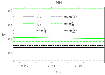
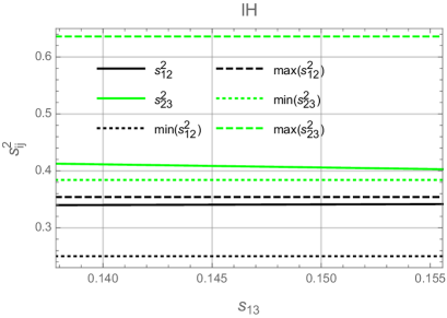
Figure 1: $s^{2}_{12}$ and $s^{2}_{23}$ as functions of $s_{13}$ in the left (right) panel for the NH (IH) case.

Figure 2: Plot of $\epsilon$ as a function of $s_{13}$. The two black dashed (blue) vertical lines show the lower and upper bounds of the 3 $\sigma$ ranges of $s_{13}$ corresponding to the NH (IH) case.

For $s_{13}^{2}$ in the 3 $\sigma$ range, it is easy to derive the allowed values of $\epsilon$,

$$\mathrm{NH:} \quad-0.376\leq\epsilon\leq-0.339,$$

$$\mathrm{IH:} \quad-0.378\leq\epsilon\leq-0.339.$$ (66)

At the best-fit point we have $\epsilon=-0.358\ (-0.359)$ for the NH (IH) case.

To estimate the allowed range of $\kappa$ and $\phi$, we use Eq. (II) to derive $m_{0}$ as a function of $\Delta m^{2}_{21}$, $s_{13}$ and $\tilde{\kappa}$,

$$m_{0}^{2}=\Delta m^{2}_{21}\left[\frac{1}{\left|\tilde{\kappa}(2+\epsilon)\right|^{2}}-\frac{1}{\left|3/2-\tilde{\kappa}\sqrt{1+\epsilon+\epsilon^{2}}\right|^{2}}\right]^{-1},$$ (67)

where $\epsilon$ and $\tilde{\kappa}$ are given by Eqs. (62) and (63), respectively. Inserting this form of $m_{0}$ into the equations in Eq. (II), we derive $m_{1,2,3}$, $\Delta m^{2}_{31}$, and $\Delta m^{2}_{23}$ as functions of $\Delta m^{2}_{21}$, $s_{13}$, $\kappa$, and $\phi$. Using the best-fit values of $\Delta m^{2}_{21}$ and $s_{13}$, we can plot $\Delta m^{2}_{31}$ ($\Delta m^{2}_{23}$) as functions of $\kappa$ with different fixed $\phi$. In Fig. 3, $\Delta m^{2}_{31}$ and $\Delta m^{2}_{23}$ corresponding to the two NH and IH cases are plotted as functions of $\kappa$ with different fixed $\phi$.

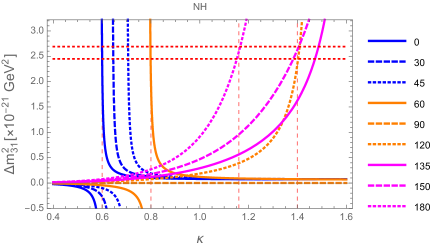
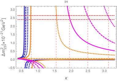
Figure 3: The left (right) panel presents $\Delta m^{2}_{31}$ ($\Delta m^{2}_{23}$) as a function of $\kappa$ with different fixed $0^{\textrm{o}}\leq\phi\leq 180^{\textrm{o}}$ in the NH (IH) case. The two red dotted lines show the 3 $\sigma$ allowed range of $\Delta m^{2}_{31}$ ($\Delta m^{2}_{23}$) corresponding to the NH (IH) case.

Here we chose the plot range of $\phi$ as $0^{\textrm{o}}\leq\phi\leq 180^{\textrm{o}}$ because the results in the range $180^{\textrm{o}}\leq\phi\leq 360^{\textrm{o}}$ are repeated. We see that with every fixed $\phi$, the respective allowed range of $\kappa$ is very narrow. In addition, the two values of $\phi=90^{\textrm{o}}$ and $270^{\textrm{o}}$ are ruled out completely for all $\kappa$ because they always result in $m_{1}=m_{3}$, leading to $\Delta m^{2}_{31}=0$ and $\Delta m^{2}_{21}=\Delta m^{2}_{23}$ ruled out by both the NH and the IH data. The allowed regions divide into three, namely $\kappa<1$ for $0^{\textrm{o}}\leq\phi<90^{\textrm{o}}$ and $270^{\textrm{o}}<\phi<360^{\textrm{o}}$, while $\kappa>1$ for $90^{\textrm{o}}<\phi<270^{\textrm{o}}$. In fact, the allowed regions are more strict because they must satisfy an additional condition that the formula of $m_{0}^{2}$ given in Eq. (67) is positive. To see how the condition $m^{2}_{0}>0$ works, we use the contour plots in Fig. 4 for the NH case, where $\Delta m^{2}_{31}$, $m^{2}_{0}$, $m_{0}$, and $m_{1}$ are functions of $\phi$ and $0.6\leq\kappa<2$, which is derived from the allowed $\kappa$ shown in Fig. 3.

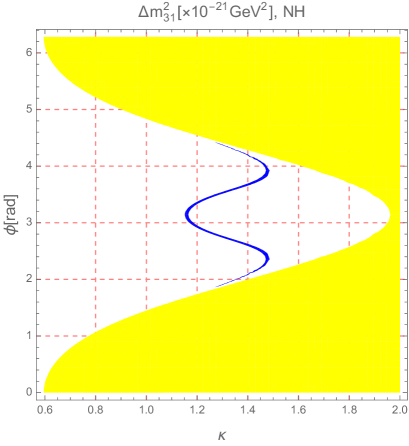
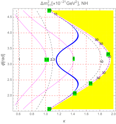
Figure 4: Contour plots of $\Delta m^{2}_{31}$ as functions of $\kappa$ and $\phi$ in the NH case. The blue regions show the 3 $\sigma$ allowed range of $\Delta m^{2}_{31}$. The yellow regions are excluded by the condition $\Delta m^{2}_{21}/m_{0}^{2}>0$. The magenta and black dashed curves in the right panel show the respective constant values of $m_{0}\times 10^{11}\ [\mathrm{GeV}]$ and $m_{1}\times 10^{12}\ [\mathrm{GeV}]$.

We can see in Fig. 4 that the allowed region is divided into two symmetric subregions by the horizontal axis $\phi=180^{\textrm{o}}$, as mentioned previously. In addition, in each subregion, for example the allowed region with $90^{\textrm{o}}<\phi<180^{\textrm{o}}$, there exists another symmetric horizontal axis $\phi=135^{\textrm{o}}$ where two values of $\phi=135^{\textrm{o}}\pm x^{\textrm{o}}$ will give the same $\Delta m^{2}_{31}$ for one fixed $\kappa$. Hence, in Fig. 3 the two lines $\phi=120^{\textrm{o}}$ and $\phi=150^{\textrm{o}}$ result in the same $\Delta m^{2}_{31}$, and the line $\phi=120<135^{\textrm{o}}$ is different from the three others lines $\phi=180^{\textrm{o}},\ 150^{\textrm{o}},\ 135^{\textrm{o}}\geq 135^{\textrm{o}}$.

Now, only the region satisfying $1.15<\kappa<1.5$ and $90^{\textrm{o}}<\phi<270^{\textrm{o}}$ are allowed for the NH case. We also roughly estimate the allowed ranges of $m_{0}$ and the lightest active neutrino mass $m_{1}$ as $0.035\ \mathrm{eV}<m_{0}<0.25\ \mathrm{eV}$ and $0.002\ \mathrm{eV}<m_{1}<0.03\ \mathrm{eV}$.

In the IH case, illustrations are shown in Fig. 5, where the contour plots are limited in two ranges of $0^{\textrm{o}}\leq\phi\leq 60^{\textrm{o}}$ and $300^{\textrm{o}}<\phi<360^{\textrm{o}}$.

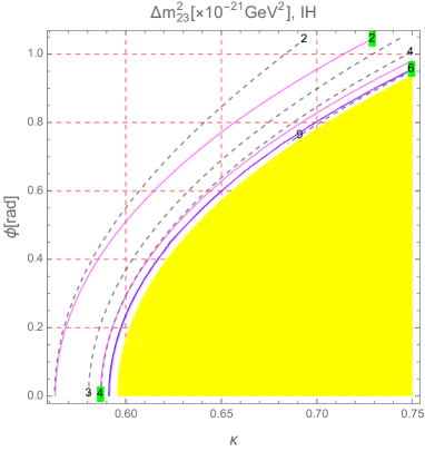
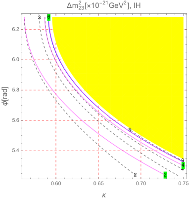
Figure 5: Contour plots of $\Delta m^{2}_{23}$ as functions of $\kappa$ and $\phi$ in the range $0\leq\phi\leq\pi/3$ (left) and $5\pi/3\leq\phi\leq 2\pi$ for the IH case. The blue regions show the 3 $\sigma$ allowed range of $\Delta m^{2}_{23}$. The yellow regions are excluded by the condition $\Delta m^{2}_{21}/m_{0}^{2}>0$. The magenta and black dashed curves in the right panel show respective constant values of $m_{0}\times 10^{11}\ [\mathrm{GeV}]$ and $m_{1}\times 10^{11}\ [\mathrm{GeV}]$.

The allowed regions satisfy that $0.5<\kappa<0.8$ and $\phi\in(0^{\textrm{o}},90^{\textrm{o}})\cup(270^{\textrm{o}},360^{\textrm{o}})$. Values of $\phi$ close to $90^{\textrm{o}}$ and $270^{\textrm{o}}$ are excluded. Indeed, the total allowed regions respecting the 3 $\sigma$ allowed range of $\Delta m^{2}_{23}$ correspond to $0^{\textrm{o}}\leq\phi<90^{\textrm{o}}$ and $270^{\textrm{o}}<\phi<360^{\textrm{o}}$. Crude estimations of $m_{0}$ and $m_{1}$ are $0.02\ \mathrm{eV}<m_{0}<0.06\ \mathrm{eV}$ and $0.04\ \mathrm{eV}<m_{1}<0.09\ \mathrm{eV}$.

Particular allowed pairs of $(\kappa,\phi)$ are collected in Tables 2 and 3 for the NH and the IH cases, respectively. This will be very convenient for investigating the LFV decays later.

Table 2: Allowed values of $(\kappa,\phi)$ generating active neutrino data in $3\sigma$ range with fixed values at best-fit points of $s_{13}^{2}=0.0215$ and $\Delta m_{21}^{2}=7.37\times 10^{-23}\text{GeV}^{2}$ in the NH case. The best-fit values and allowed ranges of $\kappa$ corresponding to every fixed $\phi$ are presented in the column two.

$\phi$	$\kappa$	$\Delta m_{31}^{2}$	$m_{0}$	$m_{1}$
[${}^{\textrm{o}}$]	best-fit, [allowed range]	$\left[\times 10^{-21}\ \text{GeV}^{2}\right]$	$\left[\times 10^{-11}\ \text{GeV}\right]$	$\left[\times 10^{-11}\ \text{GeV}\right]$
95	1.1379, [1.1377, 1.1381]	2.5785	22.744	12.143
120	1.4056, [1.4027, 1.4087]	2.5366	8.6036	3.6293
135	1.4788, [1.4720, 1.4863]	2.5593	6.0594	2.3432
150	1.3938, [1.3834, 1.4055]	2.5599	3.9809	1.5129
180	1.1582, [1.1518, 1.1654]	2.5594	2.4929	0.99067
210	1.3938, [1.3834, 1.4055]	2.5599	3.9809	1.5129
225	1.4788, [1.4720, 1.4863]	2.5593	6.0594	2.3432
240	1.4056, [1.4027, 1.4087]	2.5603	8.6447	3.6459
265	1.1379, [1.1377, 1.1381]	2.5601	22.662	12.099

In the second column of every table, the values of $\kappa$ are determined at the best-fit value and 3 $\sigma$ range of $\Delta\,m^{2}_{31}$ ($\Delta\,m^{2}_{23}$) for the NH (IH) scheme.

Comparing with previous work Karmakar:2014dva , we can see many new interesting results shown in the numerical estimation here. First, in our new approach, $\epsilon$ is investigated as a real function of $s_{13}$. Consequently, both $s^{2}_{13}$ and $s^{2}_{23}$ are also written as functions of $s_{13}$, leading to a very interesting results that these two quantities always satisfy the 3 $\sigma$ ranges. In addition, the constraint of $\epsilon$ is determined precisely from the 3 $\sigma$ allowed range of $s_{13}$. This approach also shows us clearly that the two allowed regions of the pairs $(\kappa,\phi)$ corresponding to the two NH and IH cases are completely distinguished.

Table 3: Allowed values of $(\kappa,\phi)$ generating active neutrino data in 3 $\sigma$ range with fixed values at best-fit points of $0.0216$ and $\Delta m_{21}^{2}=7.37\times 10^{-23}\ \text{GeV}^{2}$ in the IH case.

$\phi$	$\kappa$	$\Delta m_{23}^{2}$	$m_{0}$	$m_{1}$
[${}^{\textrm{o}}$]	best-fit, [allowed range]	$\left[\times 10^{-21}\ \text{GeV}^{2}\right]$	$\left[\times 10^{-11}\ \text{GeV}\right]$	$\left[\times 10^{-11}\ \text{GeV}\right]$
10	0.5960, [0.5958, 0.5962]	2.5377	5.6341	5.6958
30	0.6357, [0.6354, 0.6359]	2.6545	6.3001	5.9753
45	0.6953, [0.6950, 0.6956]	2.5293	7.0243	6.0955
60	0.7859, [0.7856, 0.7862]	2.5262	8.6822	6.6763
85	1.0207, [1.0205, 1.0208]	2.5821	22.271	13.267
275	1.0207, [1.0205, 1.0208]	2.5821	22.271	13.267
300	0.7859, [0.7856, 0.7862]	2.5262	8.6822	6.6763
315	0.6953, [0.6950, 0.6956]	2.5293	7.0243	6.0955
350	0.5960, [0.5958, 0.5962]	2.5490	5.6469	5.7088

From the above discussion, we have shown that by fixing $s_{13}$ and $\Delta m^{2}_{21}$ we can estimate the reasonable ranges of all parameters $\epsilon$, $m_{0}$, $\kappa$, and $\phi$. This is also consistent with the derivation of $m_{0}$ from the seesaw formula $m_{0}=\frac{(pv_{u})^{2}}{M_{0}}\simeq\sqrt{\Delta m^{2}_{31(23)}}\simeq 0.05$ eV for the best-fit data. We emphasize that, although our first approach for numerical investigation seems similar to that given in Ref. Adhikary:2008au , our detailed discussion added more strict conditions for $m_{0}^{2}$ and $\Delta m^{2}_{31,23}$ to show precisely the allowed ranges of $\kappa$ and $\phi$. More importantly, in the following numerical investigation we will scan the parameter space including four independent parameters $(m_{0},\ \epsilon,\,\kappa,\;\phi)$ around the ranges that have been estimated above to collect all allowed points which satisfy all of the 3 $\sigma$ experimental data of the NH or the IH cases. This method of investigation is more general than those mentioned in Refs. Adhikary:2008au ; Karmakar:2014dva . Coming back to our numerical investigation, for the NH (IH) the unknown parameters get random values in the following ranges: $0.02\ \textrm{eV}\leq m_{0}\leq 0.15\ \textrm{eV}$ ($0.05\ \textrm{eV}\leq m_{0}\leq 0.15\ \textrm{eV}$), $-0.45\leq\epsilon\leq-0.25$ ($-0.4\leq\epsilon\leq-0.32$), $1\leq\kappa\leq 1.7$ ($0.45\leq\kappa\leq 1.05$), and $0\leq\phi\leq 2\pi$. Finally, the RHN mass scale and $t_{\beta}$ are chosen as $M_{0}=10^{10}$ GeV and $t_{\beta}=3$ for the numerical investigation of $p$, which is the global parameter of the Dirac neutrino Yukawa coupling matrix $Y_{\nu}$ roughly estimated by $p^{2}\simeq\frac{M_{0}\sqrt{\Delta m^{2}_{31(23)}}}{v_{u}^{2}}$.

The parameter spaces ($\kappa,\epsilon$) and ($\phi,p$) are respectively plotted Figs 7 and 7, where the red and blue patterns represent the allowed regions of NH and the IH cases, respectively. Hereafter, we continue using these conventions unless otherwise stated.

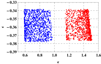
Figure 6: The allowed values of $\kappa$ and $\epsilon$ of the model. The red and blue patterns correspond to the NH and the IH of active neutrino masses, respectively.

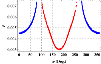
Figure 7: The correlation between the allowed values of $\phi$ and the Dirac neutrino coupling factor $p$ of the model. The roles of color patterns are the same as Fig. 7.

Note that $M_{0}$ and $t_{\beta}$ are absorbed into $m_{0}$ by the seesaw formula. As a result, the allowed regions of the parameter spaces plotted in Fig. 7 is independent from the values of $t_{\beta}$ and $M_{0}$.

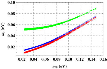
Figure 8: The active neutrino masses $m_{i}$ as a function of $m_{0}$ for the NH case.

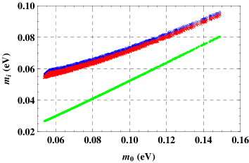
Figure 9: The active neutrino masses $m_{i}$ as a function of $m_{0}$ for the IH case.

The light neutrino masses predicted by the model are respectively plotted in Figs. 9 and 9, as functions of the light neutrino mass scale $m_{0}$ for the NH and IH cases. There, the red, blue, and green plots represent for $m_{1},\ m_{2}$, and $m_{3}$, respectively.

Figure 10: The predictions of the model for the Majorana CP-violating phases for the NH (red) and the IH (blue) cases.

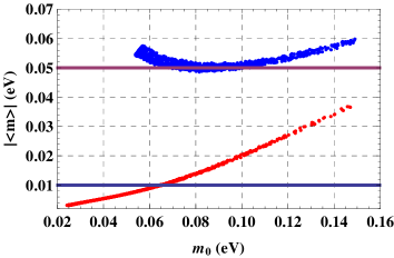
Figure 11: The predictions of the effective neutrino mass $|\langle m\rangle|$ as a function of the active neutrino mass scale $m_{0}$.

We can recognize that the neutrino masses are strong hierarchy with small values of $m_{0}$ and they can be quasi-degenerate, $m_{1}\cong m_{2}\cong m_{3}\geq 0.1$ eV Tanabashi:2018oca , if $m_{0}$ approaches above 0.15 eV. The prediction of the two Majorana CP phases is shown in Fig. 11.

It is worth to studying the effective neutrino mass in neutrinoless double beta decay ($0\nu\beta\beta$), $|\langle m\rangle|$, with the form given in Ref. Tanabashi:2018oca as

$$|\langle m\rangle| = \left|m_{1}(U_{\rm PMNS})_{e1}^{2}+m_{2}(U_{\rm PMNS})_{e2}^{2}+m_{3}(U_{\rm PMNS})_{e3}^{2}\right|$$ (68)

$$= \left|\Big{(}m_{1}c^{2}_{12}+m_{2}s^{2}_{12}e^{i\alpha_{21}}\Big{)}c^{2}_{13}+m_{3}s^{2}_{13}e^{i(\alpha_{31}-2\delta)}\right|.$$

The prediction of the effective mass $|\langle m\rangle|$ is plotted in Fig. 11 as a function of the lightest active neutrino mass $m_{0}$ for the NH (red plot) and IH (blue plot) cases. In this figure, the two horizontal lines are the prospect bounds for $|\langle m\rangle|$ of a new generation of $0\nu\beta\beta$ experiments Tanabashi:2018oca . Numerically, our predictions of $|\langle m\rangle|$ turn out to be 0.002 eV $\leq|\langle m\rangle|\leq$ 0.038 eV for NH and 0.048 eV $\leq|\langle m\rangle|\leq$ 0.058 eV for IH. Notice that the results from $0\nu 2\beta$ by KamLAND-Zen Asakura:2014lma and EXO-200 Albert:2014awa indicate an upper limit on the effective neutrino mass parameter $|\langle m\rangle|$ that $|\langle m\rangle|\leq(0.14-0.28)$ eV at $90\%$ CL. and $|\langle m\rangle|\leq(0.19-0.45)$ eV at $90\%$ CL., respectively. The most stringent upper limit now is $|\langle m\rangle|\leq(0.061-0.165)$ eV at $90\%$ CL KamLAND-Zen:2016pfg . Therefore, our result for $|\langle m\rangle|$ is still not excluded by the current experimental bounds, and we expect that our predictions for $|\langle m\rangle|$ could be measured by KamLAND-Zen and other $0\nu 2\beta$ decay experiments in their new phase which have been taking data since mid 2017; see, for the present status and future prospects, Ref. Maneschg:2017mzu . The future sensitivity can reach $|\langle m\rangle|=0.01$ eV; see a summary in Ref. Abada:2018qok , where the sensitivity of many ongoing and planned $0\nu\beta\beta$ experiments Auger:2012ar ; Albert:2014awa ; Azzolini:2018dyb ; Tosi:2014mya ; Obara:2017ndb ; Agostini:2017iyd ; Phillips:2011db ; Abgrall:2017syy ; Aguirre:2014lua ; Artusa:2014lgv ; Hartnell:2012qd ; Barabash:2011aa ; Karki:2018rhc ; Gomez-Cadenas:2013lta were listed. Because the two ranges of $|\langle m\rangle|$ predicted by the NH and IH cases are completely distinguished, $|\langle m\rangle|$ is an important channel to confirm experimentally the NH or the IH property once the effective mass $|\langle m\rangle|$ is measured. In addition, we can pin down the light neutrino mass scale $m_{0}$ and either of the active neutrino masses.

To finish the numerical investigation, we conclude some important constraints on the model parameters. The allowed ranges of the four parameters $(m_{0},\epsilon,\kappa,\phi)$ are constrained as follows. The allowed regions for the NH case are: $0.02\,\mathrm{eV}<m_{0}<0.15\,\mathrm{eV}$, $-0.038<\epsilon<-0.0345$, $1.15<\kappa<1.5$, and $90^{\text{o}}<\phi<270^{\text{o}}$. The allowed regions for the IH case are: $0.05\,\mathrm{eV}<m_{0}<0.15\,\mathrm{eV}$, $-0.038<\epsilon<-0.0345$, $0.55<\kappa<1$, $0^{\text{o}}<\phi<90^{\text{o}}$, and $270^{\text{o}}<\phi<360^{\text{o}}$. In addition, the allowed region of the light neutrino mass scale $m_{0}$ lead to upper bounds of $M_{0}$ obtained from the perturbative limit: $M_{0}=(v_{u}^{2}p)/m_{0}\leq 174^{2}\times 4\pi/(0.02\times 10^{-11})\sim O(10^{16})$ GeV. This is consistent with the GUT scale mentioned in this work.

Interestingly enough, in the next section we would like to study how the BAU can be explained by the leptogenesis scenario of the current model under the allowed regions of the parameter space discussed in this section.

III Leptogenesis

We now consider how leptogenesis can work in our scenario. The relations between heavy RHNs and active neutrino masses are derived directly from Eq. (43),

$$U_{R}^{\textrm{T}}M_{R}U_{R}={\rm diag}(M_{1},\ M_{2},\ M_{3})=(v_{u}p)^{2}~{}{\rm diag}\left(\frac{1}{m_{1}},\frac{1}{m_{2}},\frac{1}{m_{3}}\right),$$ (69)

where $U_{R}=U^{\ast}_{\rm PMNS}$ was determined precisely in the previous section. In the mass basis of the RHNs, the Dirac neutrino Yukawa coupling matrix is modified to be

$$Y_{\nu}^{\prime}=U_{R}^{\textrm{T}}Y_{\nu}=U_{\rm PMNS}^{\dagger}Y_{\nu}\Rightarrow~{}H=Y_{\nu}^{\prime}Y_{\nu}^{\prime{\dagger}}~{}=~{}p^{2}\times\textbf{1}.$$ (70)

We study the case of flavored leptogenesis, the CP asymmetry in the decay of RHN $N_{i}$ to lepton flavor $l_{\alpha}~{}(\alpha=e,\mu,\tau)$ is defined as Abada:2006ea ; Blanchet:2006be ; Antusch:2006cw ; Pascoli:2006ie ; Pascoli:2006ci ; Branco:2006ce ; Branco:2006hz

$$\varepsilon_{i}^{\alpha} = \frac{\Gamma(N_{i}\rightarrow l_{\alpha}\varphi)-\Gamma(N_{i}\rightarrow\overline{l}_{\alpha}\varphi^{{\dagger}})}{\sum_{\alpha}[\Gamma(N_{i}\rightarrow l_{\alpha}\varphi)+\Gamma(N_{i}\rightarrow\overline{l}_{\alpha}\varphi^{{\dagger}})]}$$ (71)

$$= \frac{1}{8\pi H_{ii}}\sum_{j\neq i}\Big{\{}{\rm Im}\Big{[}H_{ij}(Y^{\prime}_{\nu})_{i\alpha}(Y^{\prime}_{\nu})^{\ast}_{j\alpha}\Big{]}f\Big{(}\frac{M^{2}_{j}}{M^{2}_{i}}\Big{)},$$

where $H=Y_{\nu}^{\prime}Y_{\nu}^{\prime{\dagger}}$, and $M_{i}$ denotes the RHN masses. The loop function $f(x)$ containing the vertex and self-energy corrections is given as

$$f(x)=\sqrt{x}\Big{[}(1+x){\rm ln}\frac{x}{1+x}+\frac{2-x}{1-x}\Big{]}.$$ (72)

Notice from Eq.(71) that, in the original model, the CP asymmetry is zero due to the fact that the Hermitian matrix $H$ is proportional to the unit matrix, see Eq. (70), and a non-vanishing CP asymmetry requires ${\rm Im}[H_{ij}({Y^{\prime}}_{\nu})_{i\alpha}({Y^{\prime}}_{\nu})_{j\alpha}^{\ast}]\neq 0$. Therefore, to have leptogenesis we need to induce a non-vanishing ${H}_{ij}\ (i\neq j)$ at the leptogenesis scale. Indeed, this happens in the model under consideration because of the RG (renormalization group) effects, discussed in detail below. The RG equation for the Dirac neutrino Yukawa coupling can be written as Casas:1999tp ; Chankowski:2001mx ; Antusch:2002rr ; Branco:2005ye ; Nguyen:2012zza

$$\frac{d{Y}_{\nu}}{dt} = {Y}_{\nu}\left[\left(T-\frac{3}{4}g^{2}_{2}-\frac{9}{4}g^{2}_{1}\left)-\frac{3}{2}\right({Y}^{{\dagger}}_{l}{Y}_{l}-{Y}^{{\dagger}}_{\nu}{Y}_{\nu}\right)\right],$$ (73)

where $T=\mathrm{Tr}(3Y^{{\dagger}}_{u}Y_{u}+3Y^{{\dagger}}_{d}Y_{d}+{Y}^{{\dagger}}_{\nu}{Y}_{\nu}+{Y}^{{\dagger}}_{l}{Y}_{l})$, $Y_{u,d}$ and ${Y}_{l}$ are the Yukawa couplings of up-type and down-type quarks and charged leptons, $g_{2,1}$ are the ${\rm SU(2)}_{L}$ and ${\rm U(1)}_{Y}$ gauge coupling constants, respectively, $t=\frac{1}{16\pi^{2}}\ln(M/\Lambda^{\prime})$, and $M$ is an arbitrary renormalization scale. The cutoff scale $\Lambda^{\prime}$ can be regarded as the $G_{f}$ breaking scale $\Lambda^{\prime}=\Lambda$ and is assumed to be of the order of the GUT scale, $\Lambda^{\prime}\sim 10^{16}$ GeV.

As the structure of ${M}_{R}$ changes with the evolution of the energy scale, $U_{R}$ depends on the scale $\Lambda^{\prime}$ too. The RG evolution of $U_{R}(t)$ can be written as

$$\frac{d}{dt}U_{R}=U_{R}A,$$ (74)

where $A$ is an anti-Hermitian matrix $A^{\dagger}=-A$ due to the unitarity of $U_{R}$. The components of the $A$ matrix are given by Ahn:2006rn

$$A_{ij} = \frac{M_{j}+M_{i}}{M_{j}-M_{i}}{\rm Re}[(Y_{\nu}Y_{\nu}^{\dagger})_{ij}]+i\frac{M_{j}-M_{i}}{M_{j}+M_{i}}{\rm Im}[(Y_{\nu}Y_{\nu}^{\dagger})_{ij}].$$ (75)

The running of the RHN mass scale affects very weakly our result so we drop it here. The RG equation for $Y^{\prime}_{\nu}$ in the basis of diagonal ${M}_{R}$ is then obtained as

$$\frac{dY_{\nu}^{\prime}}{dt} = Y_{\nu}^{\prime}\left[\left(T-\frac{3}{4}g^{2}_{2}-\frac{9}{4}g^{2}_{1}\right)-\frac{3}{2}\left({Y}^{{\dagger}}_{l}{Y}_{l}-{Y}^{\prime{\dagger}}_{\nu}{Y}_{\nu}^{\prime}\right)\right]+A^{\textrm{T}}Y_{\nu}^{\prime}.$$ (76)

Finally, we obtain the RG equation for the Hermitian matrix $H=Y^{\prime}_{\nu}Y_{\nu}^{\prime{\dagger}}$ responsible for the leptogenesis as

$$\frac{dH}{dt} = 2\left(T-\frac{3}{2}g^{2}_{2}-\frac{9}{4}g^{2}_{1}\right)H-3Y_{\nu}({Y}_{l}^{\dagger}{Y}_{l})Y_{\nu}^{\prime\dagger}+3H^{2}+A^{\textrm{T}}H+HA^{\ast}.$$ (77)

With the Hermitian matrix $H$ given in Eq. (70), up to non-zero leading contributions in the right-hand side of Eq. (77), the RG is generated from the off-diagonal terms of the $H$ matrix as

$${H}_{ij}(t) \simeq -3y_{\tau}^{2}({Y}_{\nu}^{\prime})_{i3}({Y}_{\nu}^{\prime})_{j3}^{\ast}\times t.$$ (78)

The flavored CP asymmetries $\varepsilon_{i}^{\alpha}$ can then be obtained. Notice that, in this model, the tau Yukawa coupling constant ($y_{\tau}$) relates to that in the SM ($y_{\tau,\textrm{SM}}$) as $y_{\tau}^{2}=y^{2}_{\tau,\textrm{SM}}(1+t^{2}_{\beta})$. This enhances the CP asymmetries as $\varepsilon_{i}^{\alpha}\sim(1+t^{2}_{\beta})$, we will later discuss the effect of different values of $t_{\beta}$ on the numerical generation of the BAU.

After the CP asymmetry in the decay of $N_{i}$, $\varepsilon^{\alpha}_{i}$, are calculated, the final value of $\eta_{B}$ can be calculated by solving the flavor-dependent Boltzmann equations (BE). These describe the out-of-equilibrium processes such as the decay, inverse decay, and scattering involving the RHNs, as well as the non-perturbative sphaleron interaction. Besides the CP asymmetries $\varepsilon^{\alpha}_{i}$, the final value of BAU also depends on the wash-out factors $K^{\alpha}_{i}$ which measure the effects of the inverse decay of Majorana neutrino $N_{i}$ into the lepton flavor $\alpha$ and scalars. The parameter $K^{\alpha}_{i}$ is defined as Abada:2006ea

$$K^{\alpha}_{i}=\frac{\Gamma^{\alpha}_{i}}{H(M_{i})}=(Y^{\prime{\dagger}}_{\nu})_{\alpha i}(Y_{\nu}^{\prime})_{i\alpha}\frac{\upsilon^{2}_{u}}{m_{\ast}M_{i}},$$ (79)

where $\Gamma^{\alpha}_{i}$ is the partial decay width of $N_{i}$ into the lepton flavors and Higgs scalars; $H(M_{i})$ is the Hubble parameter at temperature $T=M_{i}$ defined as $H(M_{i})\simeq(4\pi^{3}g_{\ast}/45)^{\frac{1}{2}}M^{2}_{i}/M_{\textrm{Pl}}$, where $M_{\textrm{Pl}}=1.22\times 10^{19}$ GeV is the Planck mass, $g_{\ast}\simeq 116$ is the effective number of degrees of freedom of the SM with two Higgs doublets, and the equilibrium neutrino mass $m_{\ast}\simeq 10^{-3}$ eV.

Due to the flavor effects, each CP asymmetry $\varepsilon_{i}^{\alpha}$ contributes differently to the final formula for the baryon asymmetry as Abada:2006ea ; Ahn:2010cc ; Ahn:2010nw

$$\eta_{B}\simeq-2\times 10^{-2}\sum_{N_{i}}\Big{[}\varepsilon^{e}_{i}\kappa_{i}^{e}\Big{(}\frac{151}{179}K^{e}_{i}\Big{)}+\varepsilon^{\mu}_{i}\kappa_{i}^{\mu}\Big{(}\frac{344}{537}K^{\mu}_{i}\Big{)}+\varepsilon^{\tau}_{i}\kappa_{i}^{\tau}\Big{(}\frac{344}{537}K^{\tau}_{i}\Big{)}\Big{]}$$ (80)

if the RHN mass is about $M_{i}\leq(1+t^{2}_{\beta})\times 10^{9}$ GeV where the $\mu$ and $\tau$ Yukawa couplings are in equilibrium and all the flavors are to be treated separately. If $(1+t^{2}_{\beta})\times 10^{9}$ GeV $\leq M_{i}\leq(1+t^{2}_{\beta})\times 10^{12}$ GeV where only the $\tau$ Yukawa coupling is in equilibrium and treated separately while the $e$ and $\mu$ flavors are indistinguishable, then the baryon asymmetry is obtained as

$$\eta_{B}\simeq-2\times 10^{-2}\sum_{N_{i}}\Big{[}\varepsilon^{2}_{i}\kappa_{i}^{2}\Big{(}\frac{417}{589}K^{2}_{i}\Big{)}+\varepsilon^{\tau}_{i}\kappa_{i}^{\tau}\Big{(}\frac{390}{589}K^{\tau}_{i}\Big{)}\Big{]},$$ (81)

where $\varepsilon^{2}_{i}=\varepsilon^{e}_{i}+\varepsilon^{\mu}_{i}$ and $K_{i}^{2}=K_{i}^{e}+K_{i}^{\mu}$. In Eqs. (80) and (81), the wash-out factors $\kappa_{i}^{\alpha}$ are defined as

$$\kappa^{\alpha}_{i}\simeq\Big{(}\frac{8.25}{K^{\alpha}_{i}}+\Big{(}\frac{K^{\alpha}_{i}}{0.2}\Big{)}^{1.16}\Big{)}^{-1}.$$ (82)

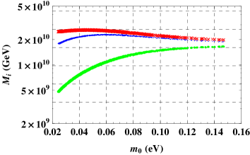
Figure 12: The RHN masses as functions of the light neutrino mass scale $m_{0}$ for the NH with $M_{0}=10^{10}$ GeV.

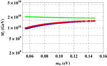
Figure 13: The RHN masses as functions of the light neutrino mass scale $m_{0}$ for the IH with $M_{0}=10^{10}$ GeV.

The allowed regions of parameter space given in Sect. II and all the formulas discussed above for $\eta_{B}$ are enough to allow us to investigate numerically the BAU predicted by the model under consideration. For $\tan\beta$ given in Eq. (7), the Lagrangian in Eq. (2) gives $v_{u}>m_{t}/\sqrt{4\pi}$. Combining with the relation in Eq. (11), it can be shown easily that $\tan\beta\geq 0.3$, which will be used in the following numerical investigations. First, the mass spectra of RHN masses as functions of the active neutrino mass scale, $m_{0}$, are plotted in Figs. 13 and 13 for the respective NH and the IH cases, where the red, blue, and green lines represent for $M_{1},\ M_{2}$ and $M_{3}$, respectively. Those RHN masses are a strong hierarchy with small values of $m_{0}$ and gradually become quasi-degenerate when $m_{0}$ approaches values around $0.15$ eV. This enhances the generated $\eta_{B}$ by the so-called resonant leptogenesis Pilaftsis:2005rv .

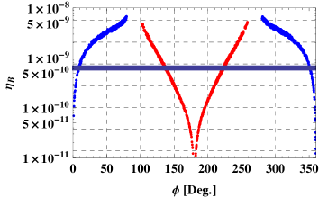
Figure 14: The prediction of $\eta_{B}$ as a function of $\phi$, where $t_{\beta}=3$ and $M_{0}=10^{10}$ GeV are used. The red (blue) curve represents the NH (IH) case.

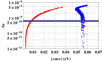
Figure 15: The correlation between $\eta_{B}$ and $|\langle m\rangle|$, where $t_{\beta}=3$ and $M_{0}=10^{10}$ GeV are used. The red (blue) curve represents the NH (IH) case.

Later, we can find in Figs. 17 and 17 that $\eta_{B}$ increases with increasing $m_{0}$ due to the effects of resonant leptogenesis. This is numerically proved in Fig. 15, where the prediction of $\eta_{B}$ as a function of the phase $\phi$ is shown. In this figure, $\eta_{B}$ gets two maxima around $\phi=90^{\textrm{o}}$ and $\phi=270^{\textrm{o}}$ for both cases of hierarchy of neutrino masses. The reason is that the parameter $p$ of the $Y_{\nu}$ matrix is proportional to $\sqrt{m_{0}}$, which has two maxima around $\phi=90^{\textrm{o}}$ and $\phi=270^{\textrm{o}}$ for both hierarchies (see, Fig. 7). Therefore, $m_{0}$, and hence $\eta_{B}$, also get their maxima around these values of the phase $\phi$. In this figure (and in Figs. 15$-$17), the solid horizontal bar represents the allowed range from experiment for BAU, namely $\eta_{B}=(6.3\pm 0.3)\times 10^{-10}$ Aghanim:2016yuo .

The correlation between $\eta_{B}$ and $|\langle m\rangle|$ is shown in Fig. 15 for $M_{0}=10^{10}$ Gev and $t_{\beta}=3$, where the red (blue) curve represents the NH (IH) case. As indicated in the previous section, once the exact value of $|\langle m\rangle|$ is confirmed we can point out the active neutrino mass scale $m_{0}$ and then we can find out the required values of the RHN mass in order to generate the right amount of $\eta_{B}$ for some given values of $t_{\beta}$.

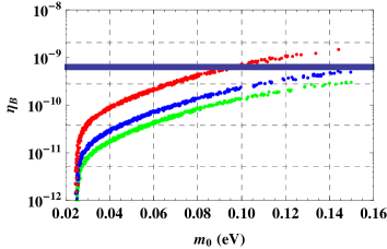
Figure 16: The prediction of $\eta_{B}$ for the case of NH as a function of the active neutrino mass scale $m_{0}$ with $M_{0}=10^{8}$ GeV. The green, blue and red plots correspond to $\tan\beta=1,3,10$, respectively.

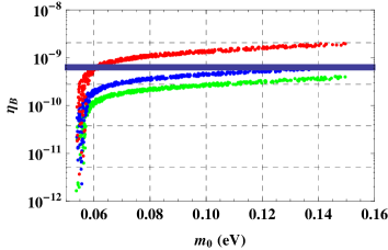
Figure 17: The prediction of $\eta_{B}$ for the case of IH as a function of the active neutrino mass scale $m_{0}$ with $M_{0}=10^{8}$ GeV. The green, blue and red plots correspond to $\tan\beta=1,3,10$, respectively.

The effects of different values of $t_{\beta}$ on the resultant of the $\eta_{B}$ are shown in Fig. 17 for NH and Fig. 17 for IH. In these figures, the green, blue, and red plots correspond to $t_{\beta}=1,\ 3$ and 10, respectively, with the mass scale of RHN $M_{0}=10^{8}$ GeV. We can find that $\eta_{B}$ increases with increasing $t_{\beta}$; with $t_{\beta}=3$ the minimum value of the mass scale $M_{0}$ is about $10^{8}$ GeV for successful leptogenesis, where the minimum values of $M_{0}$ for attaining the right value of $\eta_{B}$ are much reduced with larger values of $t_{\beta}$.

We emphasize one important point about the constraint of the heavy neutrino mass scale. For $1\leq t_{\beta}\leq 10$, our numerical investigation shows that the constraint is $O(10^{8})\ \mathrm{GeV}\leq M_{0}\leq O(10^{12})\ \mathrm{GeV}$ in order to successfully generate leptogenesis; see the illustration in Fig. 18.

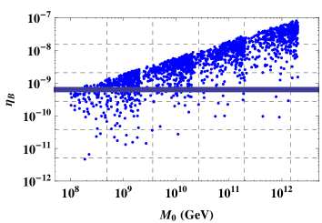
Figure 18: The prediction of $\eta_{B}$ for the case of NH (IN) as a function of the RHN mass scale $M_{0}$ with $t_{\beta}=3$ in the left (right) panel. The allowed ranges of $\kappa$, $\epsilon$, $\phi$, and $m_{0}$ summarized at the end of Sect. II are used.

This result can be explained by the fact that $M_{0}$ relates to $m_{0}$, $p$, and $v_{u}=174s_{\beta}$ through the relation in Eq. (45), where $p\leq\sqrt{4\pi}$ and the allowed $m_{0}$ is bounded as mentioned in the previous section. Our investigation shows that successful leptogenesis explained by pure RG effects requires a lower range of the RHN mass scale $M_{0}$ than other effects discussed previously, which prefer $M_{0}\geq\mathcal{O}(10^{13})$ GeV Adhikary:2008au ; Karmakar:2014dva . Therefore, the scale $M_{0}$ may be a clue to understanding which source among RG, NLO, and softterm broken $A_{4}$ successfully generates the BAU data.

Recent investigation of the SS models that can generate consistent BAU data suggest that the RHN neutrino mass scale prefers the range below $\mathcal{O}(10^{8})$ GeV Brdar:2019iem ; Brivio:2019hrj . The RHN scale is very interesting information to confirm which are the dominant sources generating consistent BAU data.

IV Lepton flavor violating decays $e_{b}\rightarrow e_{a}\gamma$

In this section we study the effects of the allowed regions of parameter space satisfying leptogenesis on LFV decays. Neutrino mixing is the only source of LFV processes. The left- and right-handed bases of the original neutral neutrinos are denoted as $\nu^{\prime}_{L}=(\nu_{L},\ (N_{R})^{c})^{\textrm{T}}$, where $\nu_{L}=(\nu_{1L},\ \nu_{2L},\ \nu_{3L})^{\textrm{T}}$ and $(N_{R})^{c}=((N_{1R})^{c},\;(N_{2R})^{c},\ (N_{3R})^{c})^{\textrm{T}}$. Also, we have $\nu^{\prime}_{R}=(\nu^{\prime}_{L})^{c}=((\nu_{L})^{c},\ N_{R})^{\textrm{T}}$. A four-component spinor for a Majorana neutrino is then $\psi=(\psi_{L},\ \psi_{R})^{\textrm{T}}$, where $\psi=\nu_{a},\ N_{a}$; $\psi_{L}=\nu_{aL},\ (N_{aR})^{c}$; and $\psi_{R}=(\nu_{aL})^{c},\ N_{aR}$. They satisfy $\psi^{c}=C\overline{\psi}^{\textrm{T}}=\psi$. The relations between a Majorana neutrino and the left- and right-handed components are $\psi_{L,R}=P_{L,R}\psi$, where $P_{L,R}=(1\mp\gamma_{5})/2$. The total mass matrix of the neutrino is

$$M^{\nu}=\left(\begin{array}[]{cc}0&m_{D}\\ m_{D}^{T}&M_{R}\\ \end{array}\right),$$ (83)

where $m_{D}$ and $M_{R}$ are given in Eqs. (15) and (32), respectively. The Lagrangian part describing the neutrino mass term is $-\frac{1}{2}\overline{\nu^{\prime}_{L}}M^{\nu}(\nu_{L}^{\prime})^{c}+\mathrm{H.c.}$ The mass matrix in Eq. (83) is diagonalized by the mixing matrix $U^{\nu}$, which is unitary and satisfies

$$U^{\nu T}M^{\nu}U^{\nu}=\hat{M}^{\nu}=\mathrm{diag}(m_{n_{1}},\;m_{n_{2}},\dots,\;m_{n_{6}})\simeq\mathrm{diag}(m_{1},\,m_{2},\,m_{3},\,M_{1},\,M_{2},\,M_{3}),$$ (84)

where the first three mass values $m_{n_{a}}$ ($a=1,2,3$) and respective eigenvectors $n_{a}$ are identified with those of active neutrinos observed by experiments. The remaining masses belong to three heavy neutrinos $n_{4,5,6}$. Hence, the last term in Eq. (84) is derived from the relations shown in Eqs. (24) and (33). The relations between the original and mass basis of the neutrino are

$$\nu^{\prime}_{iL}=U^{\nu*}_{ij}n_{jL}=U^{\nu*}_{ij}P_{L}n_{j},\hskip 14.22636pt\;\nu^{\prime}_{iR}=U^{\nu}_{ij}n_{jR}=U^{\nu}_{ij}P_{R}n_{j},$$ (85)

where $n=(n_{1},\;n_{2},\;\dots,\;n_{6})^{\textrm{T}}$ and $n_{i}=(n_{iL},\;n_{iR})^{\textrm{T}}$ ($i=1,2,\dots,6$).

Based on previous parmeterizations Casas:2001sr ; Ibarra:2010xw , the matrix $U^{\nu}$ can be written as

$$U^{\nu}=\left(\begin{array}[]{cc}I_{3}&\textbf{O}\\ \textbf{O}&U_{R}\\ \end{array}\right)\exp\left(\begin{array}[]{cc}\textbf{O}&R\\ -R^{\dagger}&\textbf{O}\\ \end{array}\right)\left(\begin{array}[]{cc}U_{\mathrm{PMNS}}&\textbf{O}\\ \textbf{O}&V_{3}\\ \end{array}\right),$$ (92)

where O is the $3\times 3$ matrix with all elements being zeros; $U_{R}$, $V_{3}$, and $U_{\mathrm{PMNS}}$ are three $3\times 3$ unitary matrices; and $R$ is a $3\times 3$ matrix satisfying $|R|\equiv\mathrm{max}[|R_{ij}|]\ll 1$ for all $i,j=1,2,3$. Apart from Eq. (23), other SS relations for determining $R$ and heavy neutrino masses are identified up to $\mathcal{O}(R^{2})$ as follows

$$R^{*} =\left(m_{D}U_{R}\right)\left[U_{R}^{\textrm{T}}M_{N}U_{R}\right]^{-1},$$

$$V^{*}_{3}\hat{M}_{R}V_{3} =U_{R}^{\textrm{T}}M_{N}U_{R}+\frac{1}{2}R^{\textrm{T}}R^{*}U_{R}^{\textrm{T}}M_{N}U_{R}+\frac{1}{2}U_{R}^{\textrm{T}}M_{N}U_{R}R^{\dagger}R,$$ (93)

where we have applied the result from Refs. Casas:2001sr ; Ibarra:2010xw , after taking a rotation of $M^{\nu}$ corresponding to the first matrix in the right-hand side of Eq. (92), which gives $m_{D}\rightarrow m_{D}U_{R}$ and $M_{R}\rightarrow U^{\textrm{T}}_{R}M_{R}U_{R}$.

In our framework, $U_{R}$ is defined from Eq. (33), and $U_{\mathrm{PMNS}}=U_{R}^{*}$ is the well-known mixing matrix of active neutrinos defined in Eq. (53). Therefore, it can be proved that

$$R^{*} =\sqrt{\frac{m_{0}}{M_{0}}}U^{*}_{\mathrm{PMNS}}\times\mathrm{diag}\left(\frac{M_{0}}{M_{1}},\,\frac{M_{0}}{M_{2}},\,\frac{M_{0}}{M_{3}}\right),$$

$$V^{*}_{3}\hat{M}_{R}V_{3} =\mathrm{diag}(M_{1},\,M_{2},\,M_{3})+\frac{m_{0}}{2}\times\mathrm{diag}\left(\frac{M_{0}}{M_{1}},\,\frac{M_{0}}{M_{2}},\,\frac{M_{0}}{M_{3}}\right)U_{\mathrm{PMNS}}U^{*}_{\mathrm{PMNS}}$$

$$+\frac{m_{0}}{2}\times U^{*}_{\mathrm{PMNS}}U_{\mathrm{PMNS}}\mathrm{diag}\left(\frac{M_{0}}{M_{1}},\,\frac{M_{0}}{M_{2}},\,\frac{M_{0}}{M_{3}}\right).$$ (94)

In the allowed region we have $\mathcal{O}(10^{-11}\ \mathrm{GeV})\sim m_{0}\ll M_{1,2,3}$, $M_{1,2,3}\geq\mathcal{O}(10^{6})\ \mathrm{GeV}$, and $M_{0}/M_{1,2,3}=\mathcal{O}(1)$, and hence the assumption mentioned above that heavy neutrino masses are given by Eq. (33) is acceptable with a very high accuracy. Using this approximation we also get $V_{3}=I_{3}$.

Up to the order $\mathcal{O}(R^{2})$, the mixing matrix $U^{\nu}$ is now

$$U^{\nu}\simeq\left(\begin{array}[]{cc}(1-\frac{1}{2}RR^{\dagger})U_{\mathrm{PMNS}}&R\\ -U^{*}_{\mathrm{PMNS}}R^{\dagger}U_{\mathrm{PMNS}}&U^{*}_{\mathrm{PMNS}}\left(1-\frac{1}{2}R^{\dagger}R\right)\\ \end{array}\right)+\mathcal{O}(R^{3}).$$ (97)

Finally, $U^{\nu}$ can be presented as a function of $M_{0},\;m_{0},\ \phi$ and $\kappa$. As we know, in the minimal model (MSS), where only heavy Dirac neutrinos are added in the SM to explain the neutrino oscillation data, the branching ratio (Br) of the LFV decay Br$(e_{b}\rightarrow e_{a}\gamma)$ was shown to be suppressed, for example Br$(\mu\rightarrow e\gamma)\leq\mathcal{O}(10^{-54})$. On the other hand, some SM extensions with heavy neutrinos obeying the SS mechanism Minkowski:1977sc ; Mohapatra:1979ia ; GellMann:1980vs ; Yanagida:1979as ; Schechter:1980gr can give large Br$(e_{b}\rightarrow e_{a}\gamma)$, close to the recent experimental sensitivities Gorbunov:2014ypa . In our model, the presence of the charged Higgs boson gives another one-loop contribution to the LFV decay amplitude. This leads to a different prediction for LFV decays that deserves to be investigated. It should be noted that, although in the model under consideration the properties of the charged Higgs boson may be the same as those discussed thoroughly in Refs. Branco:2011iw ; Hung:2019jue , the LFV couplings with neutrinos particularly, the behaviors of the LFV may be more predictive than the results of an LFV investigation for 2HDM discussed recently in Ref. Vicente:2019ykr .

In the Yukawa Lagrangian part of Eq. (1), couplings relating to LFV decays are

$$-\mathcal{L} \rightarrow \frac{m_{e_{a}}}{\sqrt{2}v_{d}}S_{d}\overline{e_{a}}e_{a}+\frac{m_{e_{a}}}{v_{d}}\left(\overline{\nu_{La}}e_{Ra}H^{+}_{d}+\mathrm{H.c.}\right)$$ (98)

$$+\frac{S_{u}}{\sqrt{2}}p\left(\overline{\nu_{aL}}N_{Ra}+\mathrm{h.c.}\right)+p\left[H^{-}_{u}\overline{e_{aL}}N_{Ra}+\mathrm{H.c.}\right].$$

Using the transformations to the physical states of the charged Higgs boson and neutrinos given respectively in Eqs. (85) and (6), the Feynman rules for LFV couplings of the charged Higgs boson are collected in Table 4. The Feynman rules for LFV coupling relating with the $W$ boson using our notation can be found in Ref. Thao:2017qtn . They are consistent with those mentioned in 2HDMs Branco:2011iw . All the Feynman rules for calculating amplitudes of LFV decays $e_{b}\rightarrow e_{a}\gamma$ in the unitary gauge are shown in Table 4. Accordingly, the one-loop calculations in this work will be done in the unitary gauge.

Table 4: Couplings relating with one-loop three-point Feynman diagrams that contribute to the LFV decay $e_{i}\rightarrow e_{j}\gamma$ in the unitary gauge.

Vertex	Coupling	Vertex	Coupling
$\overline{e_{a}}n_{i}\varphi^{-}$	$\dfrac{-igU^{\nu*}_{ai}}{m_{W}\sqrt{2}}\left(m_{e_{a}}t_{\beta}P_{L}+m_{n_{i}}t^{-1}_{\beta}P_{R}\right)$	$\overline{n_{i}}e_{a}\varphi^{+}$	$\dfrac{-igU^{\nu}_{ai}}{m_{W}\sqrt{2}}\left(m_{e_{a}}t_{\beta}P_{R}+m_{n_{i}}t^{-1}_{\beta}P_{L}\right)$
$\overline{e_{a}}n_{i}W^{-}_{\mu}$	$\dfrac{ig}{\sqrt{2}}U^{\nu*}_{ai}\gamma^{\mu}P_{L}$	$\overline{n_{i}}e_{a}W^{+}_{\mu}$	$\dfrac{ig}{\sqrt{2}}U^{\nu}_{ai}\gamma^{\mu}P_{L}$

The Br of the LFV decays $e_{b}\rightarrow e_{a}\gamma$ ($m_{e_{b}}>m_{e_{a}}$), where $(e_{b},~{}e_{a})=$ $\{(\tau,\mu),$ $(\tau,e),$ $(\mu,~{}e)\}$, can be determined as follows Lavoura:2003xp :

$$\mathrm{Br}(e_{b}\rightarrow e_{a}\gamma)=\left(1-\frac{m_{a}^{2}}{m_{b}^{2}}\right)^{3}\times\frac{12\pi^{2}}{G_{F}^{2}m_{b}^{2}}\left(|C_{L}|^{2}+|C_{R}|^{2}\right)\times\mathrm{Br}(e_{b}\rightarrow e_{a}\bar{\nu}_{a}\nu_{b}),$$ (99)

where $C_{L,R}$ are scalar factors arising from loop corrections. In the unitary gauge, one-loop Feynman diagrams contributing to $C_{L,R}$ are shown in Fig. 19.

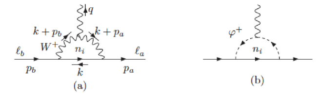
Figure 19: One-loop Feynman diagrams contributing to $C_{L,R}$ for the decay $e_{b}\rightarrow e_{a}\gamma$ in the unitary gauge.

The Br of the decay can therefore be calculated through the well-known decay rates $\tau$ or $\mu$, namely Br$(e_{b}\rightarrow e_{a}\bar{\nu}_{a}\nu_{b})$. The corresponding partial decay width is $\Gamma(e_{b}\rightarrow e_{a}\bar{\nu}_{a}\nu_{b})=\frac{G_{\textrm{F}}^{2}m^{5}_{b}}{192\pi^{3}}$ with $G_{\textrm{F}}=\frac{g^{2}\sqrt{2}}{8m^{2}_{W}}$. The experimental values are $\mathrm{Br}(\tau\rightarrow\mu\bar{\nu}_{\mu}\nu_{\tau})\simeq 17.41\%$, $\mathrm{Br}(\tau\rightarrow e\bar{\nu}_{e}\nu_{\tau})\simeq 17.83\%$, and $\mathrm{Br}(\mu\rightarrow e\bar{\nu}_{e}\nu_{\mu})\simeq 100\%$.

In the limit of zero external momenta $m_{W}^{2},m^{2}_{\varphi}\gg p_{a}^{2},p_{b}^{2}\rightarrow 0$, the analytic expressions of the amplitude are

$$C_{L,R}=C^{W}_{L,R}+C^{\varphi}_{L,R},$$ (100)

where $C^{W}_{L,R}$ and $C^{\varphi}_{L,R}$ are determined in Appendix C, consistent with Ref. Lavoura:2003xp . For low energy, Eq. (99) can be written in a more convenient form as

$$\mathrm{Br}(e_{b}\rightarrow e_{a}\gamma)=\left(1-\frac{m_{a}^{2}}{m_{b}^{2}}\right)^{3}\times\frac{3\alpha_{\mathrm{e}}}{2\pi}\left(\frac{m_{a}^{2}}{m_{b}^{2}}\left|D_{L}\right|^{2}+|D_{R}|^{2}\right)\times\mathrm{Br}(e_{b}\rightarrow\,e_{a}\bar{\nu}_{a}\nu_{b}),$$ (101)

where $C_{L,R}=\frac{g^{2}em_{a,b}}{32\pi^{2}m_{W}^{2}}\times D_{L,R}$ and $\alpha_{e}\equiv e^{2}/(4\pi)\simeq 1/137$ in numerical investigations.

Because the charged Higgs boson have similar properties to those given in the 2HDM, we set a lower bound of $300\ \mathrm{GeV}\leq m_{\varphi}\leq 2000\ \mathrm{GeV}$, and $0.3\leq t_{\beta}\leq 10$. Our investigation shows that the qualitative results of LFV decay do not change significantly, hence in the following illustration we fix $t_{\beta}=3$ and $m_{\varphi}=500$ GeV. With different pairs of $(\phi,\kappa)$ given in Table 2 satisfying all experimental data of neutrino oscillation, the dependence of LFV decay Br$(\mu\rightarrow\,e\gamma)$ on the heavy RHN mass scale $M_{0}$ is shown in Fig. 20. We constrain the lower bound of exotic neutrino masses by $M_{0}\geq\mathcal{O}(1)$ eV, leading to $|R|\sim\sqrt{\frac{m_{0}}{M_{0}}}\leq\mathcal{O}(10^{-1})$, so that the seesaw mechanism still works well.

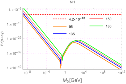
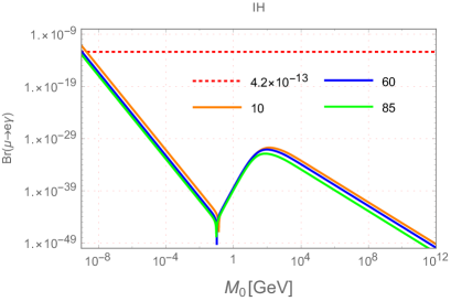
Figure 20: Br$(\mu\rightarrow\,e\gamma)$ as a function of $M_{0}$ with different allowed values of $(\phi,\kappa)$ given in Table 2 and 3 for the NH and IH cases, where the values of $\phi=95^{\textrm{o}},\;135^{\textrm{o}},\;150^{\textrm{o}},\;180^{\textrm{o}}$ or $10^{\textrm{o}},\ 60^{\textrm{o}},\ 85^{\textrm{o}}$ are pointed out in the respective figures. The red dotted lines show the experimental upper bound Br$(\mu\rightarrow\,e\gamma)<4.2\times 10^{-13}$.

The point to note is that Br$(\mu\rightarrow\,e\gamma)$ can approach the current experimental sensitivity Br$(\mu\rightarrow\,e\gamma)<4.2\times 10^{-13}$ TheMEG:2016wtm in the light exotic mass region, namely $M_{1,2,3}=\mathcal{O}(M_{0})\sim 10^{-9}-10^{-8}$ GeV. On the other hand, Br$(\mu\rightarrow\,e\gamma)$ is very suppressed with heavy $M_{i}$. Hence, if cLEV decays are detected, the region of heavy exotic neutrino masses is excluded, implying that leptogenesis and LFV data cannot be explained simultaneously in the model under consideration, i.e. the model is ruled out. We can see that the allowed region of Br$(\mu\rightarrow\,e\gamma)<4.2\times 10^{-13}$ results in very small values of Br$(\tau\rightarrow\,e\gamma)$ and Br$(\tau\rightarrow\,\mu\gamma)$; see an illustration in Figs. 21 and  22 for the HN and IH cases, respectively.

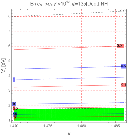
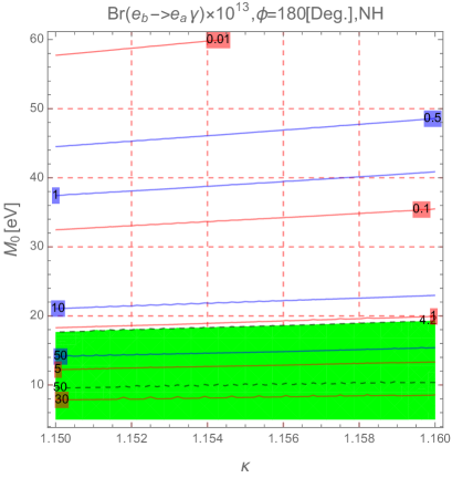
Figure 21: Contour plots of Br$(e_{b}\rightarrow\,e_{a}\gamma)$ as functions of $\kappa$ and $M_{0}$ in the NH case. The blue regions are excluded by Br$(\mu\rightarrow\,e\gamma)<4.2\times 10^{-13}$. The black dashed, red and blue curves show the constant values of Br$(\mu\rightarrow e\gamma)$, Br$(\tau\rightarrow e\gamma)$, and Br$(\tau\rightarrow\mu\gamma)$, respectively.

Generally, the constraint Br$(\mu\rightarrow e\gamma)<4.2\times 10^{-13}$ results in Br$(\tau\rightarrow\mu\gamma)\leq\mathcal{O}(10^{-12})$ and Br$(\tau\rightarrow e\gamma)\leq\mathcal{O}(10^{-13})$. These values are still much smaller than the sensitivity of near-future experiments TheMEG:2016wtm ; Baldini:2013ke ; Baldini:2019elc ; Aubert:2009ag ; Aushev:2010bq .

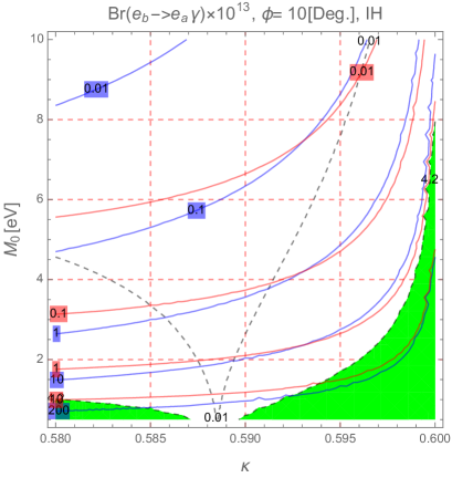
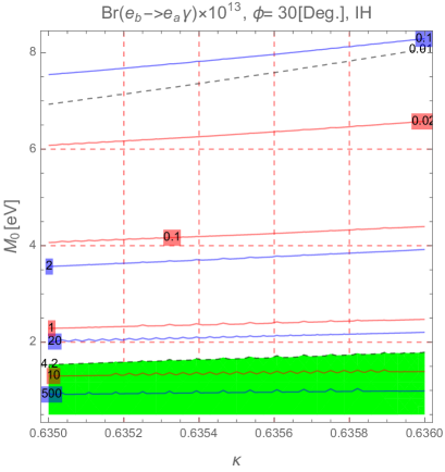
Figure 22: Contour plots of Br$(e_{b}\rightarrow\,e_{a}\gamma)$ as functions of $\kappa$ and $M_{0}$ in the NH case. The blue regions are excluded by Br$(\mu\rightarrow\,e\gamma)<4.2\times 10^{-13}$. The black dashed, red and blue curves show the constant values of Br$(\mu\rightarrow e\gamma)$, Br$(\tau\rightarrow e\gamma)$, and Br$(\tau\rightarrow\mu\gamma)$, respectively.

In most allowed regions of parameters obtained from neutrino oscillation data, all of the values of Br$(e_{b}\rightarrow\,e_{a}\gamma)$ satisfy the experimental data of LFV decay, including in the region with heavy enough RHN masses to successful explain the leptogenesis data.

In the above discussion, the neutrino mixing matrix defined in Eq. (92) is normally kept up to the order of $\mathcal{O}(R^{2})$. The results may not be accurate for very light $M_{0}$; see the illustrations for the NH case shown in Fig. 23, where higher orders of $R$ are included.

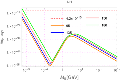
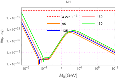
Figure 23: Plots of Br$(e_{b}\rightarrow\,e_{a}\gamma)$ as functions of $\kappa$ and $M_{0}$ in the NH case, where $U^{\nu}$ is kept up to $\mathcal{O}(R^{4})$ and $\mathcal{O}(R^{6})$ in the left and right panels, respectively.

Anyway, the Br$(\mu\rightarrow\,e\gamma)$, Br$(\tau\rightarrow\,e\gamma)$, and Br$(\tau\rightarrow\,\mu\gamma)$ are always well below the current experimental upper bounds. We note that our results predict that Br$(\mu\rightarrow e\gamma)<\mathcal{O}(10^{-29})$ with $1\,\mathrm{GeV}<M_{0}<10^{4}$ GeV. This is different from the results discussed in some previous work showing that the Br$(\mu\rightarrow\,e\gamma)$ can reach the current experimental bound Ibarra:2011xn . The reason is that the Dirac matrix mass in Ref. Ibarra:2011xn is defined following the Casas$-$Ibarra parameterization Casas:2001sr .

V Conclusion

We have studied the seesaw version of an $A_{4}$ flavor symmetry model with two Higgs singlets beside other scalars as usual $A_{4}$ models. The allowed regions of the parameter space satisfying the current experimental neutrino oscillation data at 3 $\sigma$ CL. are given numerically. We have found that the allowed ranges of $\kappa$ and $\phi$ corresponding to the NH and the IH schemes separate completely. In particular, $\phi\in(90^{\textrm{o}},270^{\textrm{o}})$ and $\kappa\in(1.15,1.5)$ are allowed for the NH case, while $\phi\in(0^{\textrm{o}},90^{\textrm{o}})\cup(270^{\textrm{o}},360^{\textrm{o}})$ and $\kappa\in(0.55,1)$ are allowed for the IH case. The model then predicts that the possible values of $|\langle m\rangle|$ will be 0.002 eV $\leq|\langle m\rangle|\leq$ 0.038 eV for the NH and 0.048 eV $\leq|\langle m\rangle|\leq$ 0.058 eV for the IH. This prediction is testable by running $0\nu 2\beta$ decay experiments, therefore is very clear information to confirm which NH or IH scheme is realistic. We have shown that the diagonal Hermitian matrix $H=Y_{\nu}Y_{\nu}^{\dagger}$ in the original model becomes non-diagonal after the effect of renormalization group evolution is included, therefore leptogenesis can be generated successfully in the allowed regions. The RHN mass scale $M_{0}=10^{8}-10^{12}$ GeV is required for successful leptogenesis. In this range, it decreases with higher values of $\tan\beta$. Illustrations for $\eta_{B}$ as functions of $m_{0}$, $\phi$, $|\langle m\rangle|$, and $M_{0}$ for different $t_{\beta}$ have been presented. The minimum value of $M_{0}$ ($10^{8}$ GeV) corresponds to the so-called resonant leptogenesis where two heavy RHN masses $M_{1}$ and $M_{3}$ are almost degenerate (and also corresponds to the maximum value of $|\langle m\rangle|$ predicted by the model). We have found an interesting correlation between $\eta_{B}$ and $|\langle m\rangle|$, so that once $|\langle m\rangle|$ is confirmed, we can pin down the RHN masses for successful leptogenesis for some given values of $\tan\beta$ as well as the absolute values of active neutrino masses.

We have also investigated the LFV decays of charged leptons, $e_{a}\rightarrow e_{b}\gamma$. Our investigation shows that if this signal is found experimentally in the future, the RHN mass scale must be smaller than the order of $\mathcal{O}(10\ \mathrm{eV})$, so that the class of models we mentioned above must be improved to explain both LFV decays and leptogenesis, or they will be ruled out.

Appendix A $A_{4}$ group: the AF (Altarelli $-$ Feruglio) basis introduced by G. Altarelli and F. Feruglio

The non-Abelian $A_{4}$ is a group of even permutations of four objects and has $4!/2=12$ elements. The group is generated by two generators $S$ and $T$ satisfying the relations

$$S^{2}=(ST)^{3}=(T^{3})=1.$$ (102)

There are three one-dimensional irreducible representations of the group denoted as

$$1: S=1,\hskip 14.22636ptT=1,$$ (103)

$$1^{\prime}: S=1,\hskip 14.22636ptT=e^{i4\pi/3}\equiv\omega^{2},$$ (104)

$$1^{\prime\prime}: S=1,\hskip 14.22636ptT=e^{i2\pi/3}\equiv\omega.$$ (105)

It is easy to check that there is no two-dimensional irreducible representation of this group. The three-dimensional unitary representations of $T$ and $S$ are given by

$$T=\left(\begin{array}[]{ccc}1&0&0\\ 0&\omega^{2}&0\\ 0&0&\omega\end{array}\right),\hskip 14.22636ptS=\frac{1}{3}{\left(\begin{array}[]{ccc}-1&2&2\\ 2&-1&2\\ 2&2&-1\end{array}\right)},$$ (112)

where $T$ has been chosen to be diagonal. The multiplication rules for the singlet and triplet representations corresponding to the above basis of two generators $T,S$ are given as

$$1\times 1=1,\ 1^{\prime}\times 1^{\prime\prime}=1,\ 3\times 3=3+3_{A}+1+1^{\prime}+1^{\prime\prime}.$$ (113)

For triplets

$$a=(a_{1},\ a_{2},\ a_{3}),\hskip 14.22636ptb=(b_{1},\ b_{2},\ b_{3}),$$ (114)

one can write

$$1\equiv(ab) = (a_{1}b_{1}+a_{2}b_{3}+a_{3}b_{2}),$$ (115)

$$1^{\prime}\equiv(ab)^{\prime} = (a_{3}b_{3}+a_{1}b_{2}+a_{2}b_{1}),$$ (116)

$$1^{\prime\prime}\equiv(ab)^{\prime\prime} = (a_{2}b_{2}+a_{1}b_{3}+a_{3}b_{1}).$$ (117)

Note that while 1 remains invariant under the exchange of the second and the third elements of $a$ and $b$, $1^{\prime}$ is symmetric under the exchange of the first and second elements while $1^{\prime\prime}$ is symmetric under the exchange of the first and third elements.

$$3 \equiv (ab)_{S}$$ (118)

$$= \frac{1}{3}(2a_{1}b_{1}-a_{2}b_{3}-a_{3}b_{2},2a_{3}b_{3}-a_{1}b_{2}-a_{2}b_{1},2a_{2}b_{2}-a_{1}b_{3}-a_{3}b_{1}),$$

$$3_{A} \equiv (ab)_{A}~{}=~{}\frac{1}{2}(a_{2}b_{3}-a_{3}b_{2},a_{1}b_{2}-a_{2}b_{1},a_{3}b_{1}-a_{1}b_{3}).$$ (119)

We will only focus only on 3 since the $3_{A}$ terms are antisymmetric and hence cannot be used for the neutrino mass matrix. In the triplet 3, we can see that the first element has 2$-$3 exchange symmetry, the second element has 1$-$2 exchange symmetry, while the third element earns 1$-$3 interchange symmetry.

Moreover, if $c,c^{\prime},c^{\prime\prime}$ are singlets of type $1,1^{\prime},1^{\prime\prime}$, and $a=(a_{1},\ a_{2},\ a_{3})$ is a triplet, then the products $ac,ac^{\prime},ac^{\prime\prime}$ are triplets explicitly given by $(a_{1}c,\ a_{2}c,\ a_{3}c)$, $(a_{3}c^{\prime},\ a_{1}c^{\prime},\ a_{2}c^{\prime})$, $(a_{2}c^{\prime\prime},\ a_{3}c^{\prime\prime},\ a_{1}c^{\prime\prime})$, respectively.

Because the above basis, $T$ is complex and $T^{*}\neq T$ in general, the complex conjugate representation $r^{*}$ of a representation $r$ ($r=1^{\prime},\ 1^{\prime\prime},\ 3$) is not the same as $r$. It is determined by the following rules Feruglio:2008ht ; Feruglio:2009hu :

$$c\sim 1\rightarrow c^{*}\sim 1,\; c^{\prime}\sim 1^{\prime}\rightarrow{c^{\prime}}^{*}\sim{1^{\prime}}^{*}=1^{\prime\prime},\;c^{\prime}\sim 1^{\prime}\rightarrow{c^{\prime\prime}}^{*}\sim{1^{\prime\prime}}^{*}=1^{\prime},$$

$$a=(a_{1},\ a_{2},\ a_{3}) \sim 3\rightarrow a^{*}=(a^{*}_{1},\ a_{3}^{*},\ a_{2}^{*}).$$ (120)

For the one-dimensional reps, it is easy to see these properties because $(\omega^{2})^{*}=\omega$. For the 3-reps we can find a transformation $U$ that changes $3^{*}$ into $3$ or $3^{*}\sim 3$ and vice versa. This is similar to the case of $SU(2)$ symmetry. Namely, $UTU^{-1}=T^{*}=T^{2}$ and $USU^{-1}=S^{*}=S$ for $T$ and $S$ given in Eq. (112). We can see this in the $S_{4}$ group where all of $T$, $T^{2}$, and $S$ are in the same conjugate class; see the details in Refs. Ishimori:2010au ; Bazzocchi:2009pv . Hence, $U$ belongs to $S_{4}$ but not $A_{4}$, namely

$$U=TSTS^{2}=\left(\begin{array}[]{ccc}1&0&0\\ 0&0&1\\ 0&1&0\\ \end{array}\right).$$ (121)

In the model considered, the $A_{4}$ lepton triplet $\overline{\psi^{l}}=(\overline{\psi^{l}_{1}},\;\overline{\psi^{l}_{2}},\;\overline{\psi^{l}_{3}})\sim 3$ has a complex conjugate of $\psi^{l}=(\psi^{l}_{1},\;\psi^{l}_{3},\;\psi^{l}_{2})\sim 3^{*}$. The $3\times 3^{*}$ is used for constructing the kinetic terms of lepton and Higgses, the Higgs potential,…For example some quadratic terms respecting $A_{4}$ symmetry are:

$$\overline{\psi^{l}} = (\overline{\psi^{l}_{1}},\;\overline{\psi^{l}_{2}},\;\overline{\psi^{l}_{3}})\sim 3,$$

$$\rightarrow \left(\overline{\psi^{l}}\gamma^{\mu}D_{\mu}\psi^{l}\right)_{1}=\overline{\psi^{l}_{1}}\gamma^{\mu}D_{\mu}\psi^{l}_{1}+\overline{\psi^{l}_{2}}\gamma^{\mu}D_{\mu}\psi^{l}_{2}+\overline{\psi^{l}_{3}}\gamma^{\mu}D_{\mu}\psi^{l}_{3},$$

$$\phi_{S} = (\phi_{S_{1}},\;\phi_{S_{2}},\;\phi_{S_{3}})\sim 3,\;\phi^{*}_{S}=(\phi^{*}_{S_{1}},\;\phi^{*}_{S_{3}},\;\phi^{*}_{S_{2}})\sim 3^{*}$$

$$\rightarrow \left((D^{\mu}\phi_{S})^{\dagger}D_{\mu}\phi_{S}\right)_{1}=(D^{\mu}\phi_{S_{1}})^{\dagger}D_{\mu}\phi_{S_{1}}+(D^{\mu}\phi_{S_{2}})^{\dagger}D_{\mu}\phi_{S_{2}}+(D^{\mu}\phi_{S_{3}})^{\dagger}D_{\mu}\phi_{S_{3}},$$

$$\left((D^{\mu}\phi_{T})^{{\dagger}}D_{\mu}\phi_{T}\right)_{1}=(D^{\mu}\phi_{T_{1}})^{\dagger}D_{\mu}\phi_{T_{1}}+(D^{\mu}\phi_{T_{2}})^{{\dagger}}D_{\mu}\phi_{T_{2}}+(D^{\mu}\phi_{T_{3}})^{{\dagger}}D_{\mu}\phi_{T_{3}},$$

$$\xi^{\prime} \sim 1^{\prime}\rightarrow{\xi^{\prime}}^{*}\sim{1^{\prime}}^{*}=1^{\prime\prime}\rightarrow({\xi^{\prime}}^{*}\xi^{\prime})_{1}={\xi^{\prime}}^{*}\xi^{\prime},\hskip 14.22636pt({\xi^{\prime\prime}}^{*}\xi^{\prime\prime})_{1}={\xi^{\prime\prime}}^{*}\xi^{\prime\prime}.$$ (122)

Note that the AF basis was used in Ref. King:2011zj .

Appendix B Higgs potential and vacuum stability

Now we come to consider the Higgs potential which satisfies the condition of $A_{4}$ invariance,

$$V_{H^{\prime}} =\mu_{1}^{2}h_{u}^{{\dagger}}h_{u}+\mu_{2}^{2}h_{d}^{{\dagger}}h_{d}+\mu_{3}^{2}\xi^{\prime{\dagger}}\xi^{\prime}+\mu_{4}^{2}\xi^{\prime\prime{\dagger}}\xi^{\prime\prime}$$

$$+\lambda_{1}(h_{u}^{{\dagger}}h_{u})^{2}+\lambda_{2}(h_{d}^{{\dagger}}h_{d})^{2}+\lambda_{3}(h_{u}^{{\dagger}}h_{u})(h_{d}^{{\dagger}}h_{d})$$

$$+\lambda_{4}(h_{u}^{{\dagger}}h_{d})(h_{d}^{{\dagger}}h_{u})+\lambda^{\xi^{\prime}}(\xi^{\prime{\dagger}}\xi^{\prime})^{2}+\lambda^{\xi^{\prime\prime}}(\xi^{\prime\prime{\dagger}}\xi^{\prime\prime})^{2}+\lambda^{\xi^{\prime}\xi^{\prime\prime}}(\xi^{{}^{\prime}\ast}\xi^{{}^{\prime}})(\xi^{{}^{\prime\prime}\ast}\xi^{{}^{\prime\prime}})$$

$$+\lambda^{u\xi^{\prime}}(h_{u}^{{\dagger}}h_{u})(\xi^{\prime\ast}\xi^{\prime})+\lambda^{d\xi^{\prime}}(h_{d}^{{\dagger}}h_{d})(\xi^{\prime\ast}\xi^{\prime})+\lambda^{u\xi^{\prime\prime}}(h_{u}^{{\dagger}}h_{u})(\xi^{\prime\prime\ast}\xi^{\prime\prime})$$

$$+\lambda^{d\xi^{\prime\prime}}(h_{d}^{{\dagger}}h_{d})(\xi^{\prime\prime\ast}\xi^{\prime\prime})$$

$$+V(\phi_{T})+V(\phi_{S})+V(\phi_{T},\phi_{S})+V(\phi_{T},h_{u})+V(\phi_{T},h_{d})$$

$$+V(\phi_{S},h_{u})+V(\phi_{S},h_{d})+V(\phi_{T},\xi^{\prime},\xi^{\prime\prime})+V(\phi_{S},\xi^{\prime},\xi^{\prime\prime}),$$ (123)

where

$$V(\phi_{T}) =\mu^{2}_{T}(\phi^{\dagger}_{T}\phi_{T})_{1}+\lambda^{\phi_{T}}_{1}(\phi^{\dagger}_{T}\phi_{T})_{1}(\phi^{\dagger}_{T}\phi_{T})_{1}+\lambda^{\phi_{T}}_{2}(\phi^{\dagger}_{T}\phi_{T})_{1^{\prime}}(\phi^{\dagger}_{T}\phi_{T})_{1^{\prime\prime}}$$

$$+\lambda^{\phi_{T}}_{3}(\phi^{\dagger}_{T}\phi_{T})_{3_{A}}(\phi^{\dagger}_{T}\phi_{T})_{3_{A}}+\lambda^{\phi_{T}}_{4}(\phi^{\dagger}_{T}\phi_{T})_{3_{S}}(\phi^{\dagger}_{T}\phi_{T})_{3_{S}}$$

$$+\lambda^{\phi_{T}}_{5}(\phi^{\dagger}_{T}\phi_{T})_{3_{S}}(\phi^{\dagger}_{T}\phi_{T})_{3_{A}},$$

$$V(\phi_{S})= \mu^{2}_{S}(\phi^{\dagger}_{S}\phi_{S})_{1}+\lambda^{\phi_{S}}_{1}(\phi^{\dagger}_{S}\phi_{S})_{1}(\phi^{\dagger}_{S}\phi_{S})_{1}+\lambda^{\phi_{S}}_{2}(\phi^{\dagger}_{S}\phi_{S})_{1^{\prime}}(\phi^{\dagger}_{S}\phi_{S})_{1^{\prime\prime}}$$

$$+\lambda^{\phi_{S}}_{3}(\phi^{\dagger}_{S}\phi_{S})_{3_{A}}(\phi^{\dagger}_{S}\phi_{S})_{3_{A}}+\lambda^{\phi_{S}}_{4}(\phi^{\dagger}_{S}\phi_{S})_{3_{S}}(\phi^{\dagger}_{S}\phi_{S})_{3_{S}}$$

$$+\lambda^{\phi_{S}}_{5}(\phi^{\dagger}_{S}\phi_{S})_{3_{S}}(\phi^{\dagger}_{S}\phi_{S})_{3_{A}},$$

$$V(\phi_{T},\phi_{S})= \lambda^{TS}_{1}(\phi^{\dagger}_{T}\phi_{T})_{1}(\phi^{\dagger}_{S}\phi_{S})_{1}+[\lambda^{TS}_{2}(\phi^{\dagger}_{T}\phi_{T})_{1^{\prime}}(\phi^{\dagger}_{S}\phi_{S})_{1^{\prime\prime}}+\textrm{H.c.}]$$

$$+\lambda^{TS}_{3}(\phi^{\dagger}_{T}\phi_{T})_{3_{A}}(\phi^{\dagger}_{S}\phi_{S})_{3_{A}}+\lambda^{TS}_{4}(\phi^{\dagger}_{T}\phi_{T})_{3_{S}}(\phi^{\dagger}_{S}\phi_{S})_{3_{S}}$$

$$+\lambda^{TS}_{5}(\phi^{\dagger}_{T}\phi_{S})_{1}(\phi^{\dagger}_{S}\phi_{T})_{1}+\lambda^{TS}_{6}(\phi^{\dagger}_{T}\phi_{S})_{1^{\prime}}(\phi^{\dagger}_{S}\phi_{T})_{1^{\prime\prime}}$$

$$+\lambda^{TS}_{7}(\phi^{\dagger}_{T}\phi_{S})_{3_{A}}(\phi^{\dagger}_{S}\phi_{T})_{3_{A}}+\lambda^{TS}_{8}(\phi^{\dagger}_{T}\phi_{S})_{3_{S}}(\phi^{\dagger}_{S}\phi_{T})_{3_{S}}$$

$$+[\lambda^{TS}_{9}(\phi^{\dagger}_{T}\phi_{S})_{3_{A}}(\phi^{\dagger}_{S}\phi_{T})_{3_{S}}+\textrm{H.c.}],$$

$$V(\phi_{T},h_{u}) =\lambda^{Tu}(\phi^{\dagger}_{T}\phi_{T})_{1}(h_{u}^{{\dagger}}h_{u}),$$

$$V(\phi_{T},h_{d}) =\lambda^{Td}(\phi^{\dagger}_{T}\phi_{T})_{1}(h_{d}^{{\dagger}}h_{d}),$$

$$V(\phi_{S},h_{u}) =\lambda^{Su}(\phi^{\dagger}_{S}\phi_{S})_{1}(h_{u}^{{\dagger}}h_{u}),$$

$$V(\phi_{S},h_{d}) =\lambda^{Sd}(\phi^{\dagger}_{S}\phi_{S})_{1}(h_{d}^{{\dagger}}h_{d}),$$

$$V(\phi_{T},\xi^{\prime},\xi^{{}^{\prime\prime}}) =\lambda_{1}^{T\xi^{\prime}\xi^{\prime}}(\phi_{T}^{{\dagger}}\phi_{T})_{1}(\xi^{\prime\ast}\xi^{\prime})+\lambda_{2}^{T\xi^{\prime\prime}\xi^{\prime\prime}}(\phi_{T}^{{\dagger}}\phi_{T})_{1}(\xi^{\prime\prime\ast}\xi^{\prime\prime})$$

$$+[\lambda_{3}^{T\xi^{\prime}\xi^{\prime\prime}}(\phi_{T}^{{\dagger}}\phi_{T})_{1^{\prime\prime}}(\xi^{\prime\ast}\xi^{\prime\prime})_{1^{\prime}}+\textrm{H.c.}],$$

$$V(\phi_{S},\xi^{\prime},\xi^{{}^{\prime\prime}}) =\lambda_{1}^{S\xi^{\prime}\xi^{\prime}}(\phi_{S}^{{\dagger}}\phi_{S})_{1}(\xi^{\prime\ast}\xi^{\prime})+\lambda_{2}^{S\xi^{\prime\prime}\xi^{\prime\prime}}(\phi_{S}^{{\dagger}}\phi_{S})_{1}(\xi^{\prime\prime\ast}\xi^{\prime\prime})$$

$$+[\lambda_{3}^{S\xi^{\prime}\xi^{\prime\prime}}(\phi_{S}^{{\dagger}}\phi_{S})_{1^{\prime\prime}}(\xi^{\prime\ast}\xi^{\prime\prime})_{1^{\prime}}+\textrm{H.c.}].$$ (124)

There are ten neutral Higgs components in the model, implying ten equations for the minimal condition of the Higgs potential in Eq. (123). But only nine equations are independent of each other, namely

$$\mu_{1}^{2}+\lambda^{u\xi^{\prime}}u^{\prime 2}+\lambda^{u\xi^{\prime\prime}}u^{\prime\prime 2}+\lambda_{3}v_{d}^{2}+3\lambda^{Su}v_{S}^{2}+\lambda^{Tu}v_{T}^{2}+2\lambda_{1}v_{u}^{2}=0,$$

$$\mu_{2}^{2}+\lambda^{d\xi^{\prime}}u^{\prime 2}+\lambda^{d\xi^{\prime\prime}}u^{\prime\prime 2}+2\lambda_{2}v_{d}^{2}+3\lambda^{Sd}v_{S}^{2}+\lambda^{Td}v_{T}^{2}+\lambda_{3}v_{u}^{2}=0,$$

$$\mu_{3}^{2}u^{\prime}+2\lambda^{\xi^{\prime}}u^{\prime 3}+\lambda^{\xi^{\prime}\xi^{\prime\prime}}u^{\prime}u^{\prime\prime 2}+\lambda^{d\xi^{\prime}}u^{\prime}v_{d}^{2}+3\lambda_{1}^{S\xi^{\prime}\xi^{\prime}}u^{\prime}v_{S}^{2}+3\lambda_{3}^{S\xi^{\prime}\xi^{\prime\prime}}u^{\prime\prime}v_{S}^{2}$$

$$+\ \lambda_{1}^{T\xi^{\prime}\xi^{\prime}}u^{\prime}v_{T}^{2}+\lambda^{u\xi^{\prime}}u^{\prime}v_{u}^{2}=0,$$

$$\mu_{4}^{2}u^{\prime\prime}+2\lambda^{\xi^{\prime\prime}}u^{\prime\prime 3}+\lambda^{\xi^{\prime}\xi^{\prime\prime}}u^{\prime 2}u^{\prime\prime}+\lambda^{d\xi^{\prime\prime}}u^{\prime\prime}v_{d}^{2}+3\lambda_{3}^{S\xi^{\prime}\xi^{\prime\prime}}u^{\prime}v_{S}^{2}+3\lambda_{2}^{S\xi^{\prime\prime}\xi^{\prime\prime}}u^{\prime\prime}v_{S}^{2}$$

$$+\ \lambda_{2}^{T\xi^{\prime\prime}\xi^{\prime\prime}}u^{\prime\prime}v_{T}^{2}+\lambda^{u\xi^{\prime\prime}}u^{\prime\prime}v_{u}^{2}=0,$$

$$\mu_{T}^{2}+\lambda_{1}^{T\xi^{\prime}\xi^{\prime}}u^{\prime 2}+\lambda_{2}^{T\xi^{\prime\prime}\xi^{\prime\prime}}u^{\prime\prime 2}+\lambda^{Td}v_{d}^{2}+3\lambda_{1}^{ST}v_{S}^{2}+\lambda_{5}^{ST}v_{S}^{2}$$

$$+\ \lambda_{6}^{ST}v_{S}^{2}+2\lambda_{7}^{ST}v_{S}^{2}+6\lambda_{8}^{ST}v_{S}^{2}+2\lambda_{1}^{T}v_{T}^{2}+8\lambda_{4}^{T}v_{T}^{2}+\lambda^{Tu}v_{u}^{2}=0,$$

$$\lambda_{3}^{T\xi^{\prime}\xi^{\prime\prime}}u^{\prime}u^{\prime\prime}+3\lambda_{2}^{ST}v_{S}^{2}+\lambda_{5}^{ST}v_{S}^{2}+\lambda_{6}^{ST}v_{S}^{2}-\lambda_{7}^{ST}v_{S}^{2}-3\lambda_{8}^{ST}v_{S}^{2}=0,$$

$$\mu_{S}^{2}+\lambda_{1}^{S\xi^{\prime}\xi^{\prime}}u^{\prime 2}+\lambda_{3}^{S\xi^{\prime}\xi^{\prime\prime}}u^{\prime}u^{\prime\prime}+\lambda_{2}^{S\xi^{\prime\prime}\xi^{\prime\prime}}u^{\prime\prime 2}+\lambda^{Sd}v_{d}^{2}+6\lambda_{1}^{ST}v_{S}^{2}+6\lambda_{2}^{S}v_{S}^{2}$$

$$+\ \lambda_{1}^{ST}v_{T}^{2}+4\lambda_{4}^{ST}v_{T}^{2}+\ \lambda_{5}^{ST}v_{T}^{2}+4\lambda_{8}^{ST}v_{T}^{2}+\lambda^{Su}v_{u}^{2}=0,$$

$$\mu_{S}^{2}+\lambda_{1}^{S\xi^{\prime}\xi^{\prime}}u^{\prime 2}+2\lambda_{3}^{S\xi^{\prime}\xi^{\prime\prime}}u^{\prime}u^{\prime\prime}+\lambda_{2}^{S\xi^{\prime\prime}\xi^{\prime\prime}}u^{\prime\prime 2}+\lambda^{Sd}v_{d}^{2}+6\lambda_{1}^{S}v_{S}^{2}+6\lambda_{2}^{S}v_{S}^{2}$$

$$+\ \lambda_{1}^{ST}v_{T}^{2}-2\lambda_{4}^{ST}v_{T}^{2}+\lambda_{6}^{ST}v_{T}^{2}+\lambda_{7}^{ST}v_{T}^{2}+\lambda_{8}^{ST}v_{T}^{2}-2\lambda_{9}^{ST}v_{T}^{2}+\lambda^{Su}v_{u}^{2}=0,$$

$$\mu_{S}^{2}+\lambda_{1}^{S\xi^{\prime}\xi^{\prime}}u^{\prime 2}+2\lambda_{3}^{S\xi^{\prime}\xi^{\prime\prime}}u^{\prime}u^{\prime\prime}+\lambda_{2}^{S\xi^{\prime\prime}\xi^{\prime\prime}}u^{\prime\prime 2}+\lambda^{Sd}v_{d}^{2}+6\lambda_{1}^{S}v_{S}^{2}+6\lambda_{2}^{S}v_{S}^{2}$$

$$+\ \lambda_{1}^{ST}v_{T}^{2}-2\lambda_{4}^{ST}v_{T}^{2}+\lambda_{7}^{ST}v_{T}^{2}+\lambda_{8}^{ST}v_{T}^{2}+2\lambda_{9}^{ST}v_{T}^{2}+\lambda^{Su}v_{u}^{2}=0.$$

These correspond to nine dependent parameters which are represented as functions of the remaining parameters in the Higgs potential, including the VEVs of neutral Higgs components. The nine dependent parameters chosen in this work are $\mu^{2}_{1}$, $\mu^{2}_{2}$, $\mu^{2}_{3}$, $\mu^{2}_{4}$, $\mu^{2}_{T}$, $\mu^{2}_{S}$, $\lambda_{4}^{ST}$, $\lambda_{6}^{ST}$, and $\lambda_{3}^{T\xi^{\prime}\xi^{\prime\prime}}$. Inserting them into Eq. (123), the Higgs potential contains only independent parameters. The assumed vacuum aligments given in Table 1 satisfy the above minimal equations, hence this assumption can be dynamically achieved. Now, we can find the masses and mass eigenstates of Higgs bosons predicted by the model.

Regarding CP-odd neutral Higgs components, it is easily shown that the squared mass matrix has a zero determinant, which implies exactly a massless sate corresponding to the Goldstone boson of the $Z$ boson in the SM. On the other hand, this model must contain at least one SM-like Higgs bosons observed by the LHC. Hence, the squared mass matrix of the CP-even neutral Higgs bosons must contain this Higgs boson. The squared mass matrix of the CP-even Higgs components is a $10\times 10$ matrix with a large number of Higgs self-couplings which are independent parameters. In this work we will choose a simple case of the Higgs potential that makes the Higgs spectrum realistic. In other words, the Higgs potential must satisfy the following conditions: (i) boundedness from below (BFB) and vacuum stability, (ii) all masses of physical Higgs are positive, (iii) having an SM-like Higgs boson observed by the LHC. Here we will focus mainly on the identification of an SM-like Higgs boson.

In general, the squared mass matrix of the CP-even Higgs bosons are a $10\times 10$ matrix, where the main contribution to the SM-like Higgs boson arises from the two Higgs doublets $h_{u}$ and $h_{d}$. Hence, we will choose the regime that these Higgs doublets decouple to other Higgs singlets, namely

$$\lambda^{u\xi^{\prime}}=\lambda^{d\xi^{\prime}}=\lambda^{u\xi^{\prime\prime}}=\lambda^{d\xi^{\prime\prime}},\hskip 14.22636pt\lambda^{Tu}=\lambda^{Td}=\lambda^{Su}=\lambda^{Sd}=0.$$ (125)

With this choice, the mass matrix will separate into two submatrices, a $2\times 2$ and an $8\times 8$. The $8\times 8$ matrix gives eight physical heavy Higgs bosons with masses depending on heavy VEVs $v_{S}$ and $v_{T}$. In the original basis $(S_{u},\;S_{d})^{\textrm{T}}$, the $2\times 2$ matrix contains an SM-like Higgs boson and has the form

$$M^{2}_{1}=\left(\begin{array}[]{cc}4\lambda_{1}v_{u}^{2}&2\lambda_{3}v_{u}v_{d}\\ 2\lambda_{3}v_{u}v_{d}&4\lambda_{2}v_{d}^{2}\\ \end{array}\right).$$ (128)

This gives two mass eigenstates, denoted as $H_{1}$ and $H_{2}$. Their masses and relations with the original states are

$$m^{2}_{H_{1}}=2v^{2}c^{2}_{\beta}\left[\lambda_{1}t_{\beta}^{2}+\lambda_{2}-\sqrt{\left(\lambda_{1}t^{2}_{\beta}-\lambda_{2}\right)^{2}+\lambda_{3}^{2}t^{2}_{\beta}}\right],\;H_{1}=S_{u}c_{\alpha}-S_{d}s_{\alpha},$$

$$m^{2}_{H_{2}}=2v^{2}c^{2}_{\beta}\left[\lambda_{1}t_{\beta}^{2}+\lambda_{2}+\sqrt{\left(\lambda_{1}t^{2}_{\beta}-\lambda_{2}\right)^{2}+\lambda_{3}^{2}t^{2}_{\beta}}\right],\;H_{2}=S_{u}s_{\alpha}+S_{d}c_{\alpha},$$ (129)

where $s_{\alpha}\equiv\sin\alpha$, $c_{\alpha}\equiv\cos\alpha$, $s_{2\alpha}\equiv\sin 2\alpha$, and

$$\tan 2\alpha=\dfrac{\lambda_{3}t_{\beta}}{\lambda_{2}-\lambda_{1}t^{2}_{\beta}}.$$ (130)

In the limit $\beta=\alpha+\pi/2$, we can show that the couplings of $H_{1}$ with other SM particles are the same as the SM predictions. Hence, in our model $H_{1}$ is identified with the SM-like Higgs boson found experimentally.

Regarding CP-odd neutral Higgs components, it is easily shown that the squared mass matrix has a zero determinant, which implies exactly a massless sate corresponding to the Goldstone boson of the $Z$ boson in the SM. Nine other CP-odd neutral Higgs are irrelevant to the phenomenology mentioned in this work.

Appendix C Passarino$-$Veltman functions for LFV decays $e_{b}\rightarrow e_{a}\gamma$ ($b>a$)

The Passarino$-$Veltman functions, called $C$-functions, are defined as follows:

$$C_{0,\mu,\mu\nu}(M_{1},M_{2},M_{2})\equiv\frac{1}{i\pi^{2}}\int\frac{d^{4}k\times\{1,k_{\mu},k_{\mu\nu}\}}{D_{0}D_{1}D_{2}},$$ (131)

where $D_{0}=k^{2}-M_{1}^{2},\;D_{1}=(k+p_{b})^{2}-M_{2}^{2}$, and $D_{2}=(k+p_{a})^{2}-M_{2}^{2}$, where $p_{b}\equiv\,p_{1}$ and $p_{a}\equiv p_{2}$ in usual notations for definitions of $C_{0,i,ij}$. The scalar $C$-functions are defined as $C_{\mu}=C_{1}p_{b\mu}+C_{2}p_{a\mu}$ and $C_{\mu\nu}=C_{00}g_{\mu\nu}+C_{11}p_{b\mu}p_{b\nu}+C_{12}(p_{b\mu}p_{a\nu}+p_{b\nu}p_{a\mu})+C_{22}p_{a\mu}p_{a\nu}$. For LFV decay processes $e_{b}\rightarrow e_{a}\gamma$ we denote $p_{a,b}^{2}=m_{a,b}^{2}$, where $m_{a,b}$ are the masses of the charged leptons $e_{a,b}$. The momentum of the photon $q=p_{b}-p_{a}$ satisfies $(p_{b}-p_{a})^{2}=q^{2}=0$. The $C$-functions in this case are,

$$C_{0} = \frac{t-1-t\ln t}{M_{2}^{2}(t-1)^{2}},\;C_{1}=C_{2}=-\frac{3t^{2}-4t+1-2t^{2}\ln t}{4(t-1)^{3}M_{2}^{2}},$$

$$C_{11} = C_{22}=2C_{12}=\frac{11t^{3}-18t^{2}+9t-2-6t^{3}\ln t}{18M_{2}^{2}(t-1)^{4}},$$ (132)

where $t=M_{1}^{2}/M_{2}^{2}$. With $t=1$, we have $C_{0}=-1/(2M_{2}^{2})$, $C_{1}=1/(6M_{2}^{2})$ and $C_{11}=-1/(12M_{2}^{2})$.

The definition of derivatives in Eq. (8) results in the definition of the tensor strength of gauge bosons as $F^{a}_{\mu\nu}=\partial_{\mu}W^{a}_{\nu}-\partial_{\nu}W^{a}_{\mu}+g\epsilon_{abc}W^{b}_{\mu}W^{c}_{\nu}$. The couplings of the photon to $W^{\pm}$ and $\phi^{\pm}$ are then determined as follows:

$$A_{\mu}\varphi^{+}\varphi^{-}: \ ie(p_{+}-p_{-})^{\mu},$$

$$A_{\lambda}W^{+}_{\mu}W^{-}_{\nu}: \ -ie\left[g^{\lambda\mu}\left(q-p_{+}\right)^{\nu}+g^{\mu\nu}\left(p_{+}-p_{-}\right)^{\lambda}+g^{\nu\lambda}\left(p_{-}-q\right)^{\mu}\right]$$ (133)

where $q$ and $p_{\pm}$ denote incoming photon momenta and $\varphi^{\pm}(W^{\pm})$, respectively.

Contributions from $W$ and $\varphi^{\pm}$ bosons to $C_{L,R}$ are calculated based on the general form given in Ref. Hue:2017lak ,

$$C^{W}_{L} = -\frac{eg^{2}m_{a}}{32\pi^{2}m_{W}^{2}}\sum_{i=1}^{6}U^{\nu}_{bi}U^{\nu*}_{ai}\left[2(C_{12}+C_{22}-C_{1})m_{W}^{2}+m_{b}^{2}(C_{11}+C_{12}+C_{1})\right.$$

$$\left.+m_{n_{i}}^{2}(C_{0}+C_{1}+2C_{2}+C_{12}+C_{22})\right],$$

$$C^{W}_{R} = -\frac{eg^{2}m_{b}}{32\pi^{2}m_{W}^{2}}\sum_{i=1}^{6}U^{\nu}_{bi}U^{\nu*}_{ai}\left[2(C_{11}+C_{12}-C_{2})m_{W}^{2}+m_{a}^{2}(C_{12}+C_{22}+C_{2})\right.$$ (134)

$$\left.+m_{n_{i}}^{2}(C_{0}+2C_{1}+C_{2}+C_{11}+C_{12})\right]$$

with $C_{0,a,ab}=C_{0,a,ab}(m_{n_{i}},m_{W},m_{W})$, and

$$C^{\varphi}_{L}=-\frac{m_{a}eg^{2}}{32\pi^{2}m^{2}_{W}}\sum_{i=1}^{6}U^{\nu*}_{ai}U^{L}_{bi} \times \left\{t_{\beta}^{2}m^{2}_{b}(C_{1}+C_{11}+C_{12})\right.$$

$$+ \left.m^{2}_{n_{i}}\left[t_{\beta}^{-2}\left(C_{2}+C_{12}+C_{22}\right)-(C_{0}+C_{1}+C_{2})\right]\right\},$$

$$C^{\varphi}_{R}=-\frac{m_{b}eg^{2}}{32\pi^{2}m^{2}_{W}}\sum_{i=1}^{6}U^{\nu*}_{ai}U^{L}_{bi} \times \left\{t_{\beta}^{2}m^{2}_{a}(C_{2}+C_{12}+C_{22})\right.$$ (135)

$$+ \left.m^{2}_{n_{i}}\left[t_{\beta}^{-2}\left(C_{1}+C_{11}+C_{12}\right)-(C_{0}+C_{1}+C_{2})\right]\right\}$$

with $C_{0,a,ab}=C_{0,a,ab}(m_{n_{i}},m_{\varphi},m_{\varphi})$.

The formula for $C^{W}_{L,R}$ is consistent with that given in Refs. He:2002pva ; Ibarra:2011xn ; Dinh:2012bp ; Petcov:2013poa in the limit $m_{a},m_{b}<<m_{W}$ and $t_{W,i}\equiv\frac{m^{2}_{n_{i}}}{m^{2}_{W}}$, namely

$$\frac{C^{W}_{L}}{m_{a}}=\frac{C^{W}_{R}}{m_{b}}=-\frac{g^{2}e}{32\pi^{2}m_{W}^{2}}f_{V}(t_{Wi}),\quad f_{V}(t)=-\frac{10-43t+78t^{2}-49t^{3}+4t^{4}+18t^{3}\ln t}{12\left(t-1\right)^{4}}.$$ (136)

In the limit $m_{a,b}\rightarrow 0$ with $t_{\beta}=1$ and $t_{\varphi,i}=\frac{m^{2}_{n_{i}}}{m^{2}_{\varphi}}$, the contributions from the charged Higgs bosons $C^{\varphi}_{L,R}$ have the following forms:

$$\frac{C^{\varphi}_{L}}{m_{a}}=\frac{C^{\varphi}_{R}}{m_{b}}=-\frac{g^{2}e}{32\pi^{2}m_{W}^{2}}f_{s}(t_{\varphi,i}),\quad f_{s}(t)\equiv\frac{t\left[7-12t-3t^{2}+8t^{3}-6t\left(-2+3t\right)\ln t\right]}{12\left(t-1\right)^{4}}.$$ (137)

References

- (1) P. F. Harrison, D. H. Perkins and W. G. Scott, Phys. Lett. B 530 (2002) 167 [hep-ph/0202074].
- (2) P. F. Harrison and W. G. Scott, Phys. Lett. B 535, 163 (2002) [hep-ph/0203209].
- (3) P. F. Harrison and W. G. Scott, Phys. Lett. B 547 (2002) 219 [hep-ph/0210197].
- (4) P. F. Harrison and W. G. Scott, Phys. Lett. B 557, 76 (2003) [hep-ph/0302025].
- (5) E. Ma and G. Rajasekaran, Phys. Rev. D 64, 113012 (2001) [hep-ph/0106291].
- (6) K. S. Babu, E. Ma and J. W. F. Valle, Phys. Lett. B 552 (2003) 207 [hep-ph/0206292].
- (7) G. Altarelli and F. Feruglio, Nucl. Phys. B 720 (2005) 64 [hep-ph/0504165].
- (8) G. Altarelli and F. Feruglio, Nucl. Phys. B 741 (2006) 215 [hep-ph/0512103].
- (9) F. Bazzocchi, S. Kaneko and S. Morisi, JHEP 0803 (2008) 063 [arXiv:0707.3032 [hep-ph]].
- (10) B. Brahmachari, S. Choubey and M. Mitra, Phys. Rev. D 77 (2008) 073008 Erratum: [Phys. Rev. D 77 (2008) 119901] [arXiv:0801.3554 [hep-ph]].
- (11) B. Adhikary and A. Ghosal, Phys. Rev. D 78 (2008) 073007 [arXiv:0803.3582 [hep-ph]].
- (12) F. Feruglio, C. Hagedorn, Y. Lin and L. Merlo, Nucl. Phys. B 775 (2007) 120 Erratum: [Nucl. Phys. B 836 (2010) 127] [hep-ph/0702194].
- (13) M. C. Chen and K. T. Mahanthappa, Phys. Lett. B 652 (2007) 34 [arXiv:0705.0714 [hep-ph]].
- (14) P. H. Frampton and T. W. Kephart, JHEP 0709 (2007) 110 doi:10.1088/1126-6708/2007/09/110 [arXiv:0706.1186 [hep-ph]].
- (15) P. H. Frampton and S. Matsuzaki, Phys. Lett. B 679 (2009) 347 [arXiv:0902.1140 [hep-ph]].
- (16) S. Pakvasa and H. Sugawara, Phys. Lett. 82B (1979) 105.
- (17) T. Brown, N. Deshpande, S. Pakvasa and H. Sugawara, Phys. Lett. 141B (1984) 95.
- (18) D. G. Lee and R. N. Mohapatra, Phys. Lett. B 329 (1994) 463 [hep-ph/9403201].
- (19) E. Ma, Phys. Lett. B 632 (2006) 352 [hep-ph/0508231].
- (20) M. Tanabashi et al. [Particle Data Group], Phys. Rev. D 98 (2018) no.3, 030001.
- (21) G. Altarelli, F. Feruglio and L. Merlo, Fortsch. Phys. 61 (2013) 507 [arXiv:1205.5133 [hep-ph]].
- (22) E. Ma, Phys. Rev. D 86 (2012) 117301 [arXiv:1209.3374 [hep-ph]].
- (23) Y. H. Ahn, S. K. Kang and C. S. Kim, Phys. Rev. D 87 (2013) no.11, 113012 [arXiv:1304.0921 [hep-ph]].
- (24) M. C. Chen, J. Huang, J. M. O’Bryan, A. M. Wijangco and F. Yu, JHEP 1302 (2013) 021 [arXiv:1210.6982 [hep-ph]].
- (25) P. P. Novichkov, S. T. Petcov and M. Tanimoto, Phys. Lett. B 793 (2019) 247 [arXiv:1812.11289 [hep-ph]].
- (26) G. J. Ding, S. F. King and X. G. Liu, JHEP 1909 (2019) 074 [arXiv:1907.11714 [hep-ph]].
- (27) B. Karmakar and A. Sil, Phys. Rev. D 93 (2016) no.1, 013006 [arXiv:1509.07090 [hep-ph]].
- (28) S. Morisi, D. V. Forero, J. C. Romão and J. W. F. Valle, Phys. Rev. D 88 (2013) no.1, 016003 [arXiv:1305.6774 [hep-ph]].
- (29) B. Karmakar and A. Sil, Phys. Rev. D 91 (2015) 013004 [arXiv:1407.5826 [hep-ph]].
- (30) J. Barry and W. Rodejohann, Phys. Rev. D 81 (2010) 093002 Erratum: [Phys. Rev. D 81 (2010) 119901] [arXiv:1003.2385 [hep-ph]].
- (31) P. Minkowski, Phys. Lett. 67B (1977) 421.
- (32) R. N. Mohapatra and G. Senjanovic, Phys. Rev. Lett. 44 (1980) 912.
- (33) M. Gell-Mann, P. Ramond and R. Slansky, Conf. Proc. C 790927 (1979) 315 [arXiv:1306.4669 [hep-th]].
- (34) T. Yanagida, Conf. Proc. C 7902131 (1979) 95.
- (35) J. Schechter and J. W. F. Valle, Phys. Rev. D 22 (1980) 2227.
- (36) M. Fukugita and T. Yanagida, Phys. Lett. B 174 (1986) 45.
- (37) G. F. Giudice, A. Notari, M. Raidal, A. Riotto and A. Strumia, Nucl. Phys. B 685 (2004) 89 [hep-ph/0310123].
- (38) W. Buchmuller, P. Di Bari and M. Plumacher, Annals Phys. 315 (2005) 305 [hep-ph/0401240].
- (39) S. M. Bilenky, S. Pascoli and S. T. Petcov, Phys. Rev. D 64 (2001) 053010 [hep-ph/0102265].
- (40) S. Pascoli, S. T. Petcov and L. Wolfenstein, Phys. Lett. B 524 (2002) 319 doi:10.1016/S0370-2693(01)01403-4 [hep-ph/0110287].
- (41) S. Pascoli, S. T. Petcov and W. Rodejohann, Phys. Lett. B 549 (2002) 177 [hep-ph/0209059].
- (42) S. T. Petcov, New J. Phys. 6 (2004) 109.
- (43) C. D. Froggatt and H. B. Nielsen, Nucl. Phys. B 147 (1979) 277. doi:10.1016/0550-3213(79)90316-X
- (44) G. Aad et al. [ATLAS Collaboration], Phys. Lett. B 716 (2012) 1 [arXiv:1207.7214 [hep-ex]].
- (45) S. Chatrchyan et al. [CMS Collaboration], Phys. Lett. B 716 (2012) 30 [arXiv:1207.7235 [hep-ex]].
- (46) K. Asakura et al. [KamLAND-Zen Collaboration], AIP Conf. Proc. 1666 (2015) no.1, 170003 [arXiv:1409.0077 [physics.ins-det]].
- (47) J. B. Albert et al. [EXO-200 Collaboration], Nature 510 (2014) 229 [arXiv:1402.6956 [nucl-ex]].
- (48) A. Gando et al. [KamLAND-Zen Collaboration], Phys. Rev. Lett. 117 (2016) no.8, 082503 Addendum: [Phys. Rev. Lett. 117 (2016) no.10, 109903] [arXiv:1605.02889 [hep-ex]].
- (49) W. Maneschg, “Present status of neutrinoless double beta decay searches,” arXiv:1704.08537 [physics.ins-det].
- (50) A. Abada, Á. Hernández-Cabezudo and X. Marcano, JHEP 1901 (2019) 041 [arXiv:1807.01331 [hep-ph]].
- (51) M. Auger et al. [EXO-200 Collaboration], Phys. Rev. Lett. 109 (2012) 032505 [arXiv:1205.5608 [hep-ex]].
- (52) O. Azzolini et al. [CUPID-0 Collaboration], Phys. Rev. Lett. 120 (2018) no.23, 232502 [arXiv:1802.07791 [nucl-ex]].
- (53) D. Tosi [EXO-200 Collaboration], doi:10.1142/9789814603164_0047 arXiv:1402.1170 [nucl-ex].
- (54) S. Obara [KamLAND-Zen Collaboration], Nucl. Instrum. Meth. A 845 (2017) 410.
- (55) M. Agostini et al., Nature 544 (2017) 47 [arXiv:1703.00570 [nucl-ex]].
- (56) D. G. Phillips, II et al., J. Phys. Conf. Ser. 381 (2012) 012044 [arXiv:1111.5578 [nucl-ex]].
- (57) N. Abgrall et al. [LEGEND Collaboration], AIP Conf. Proc. 1894 (2017) no.1, 020027 [arXiv:1709.01980 [physics.ins-det]].
- (58) D. R. Artusa et al. [CUORE Collaboration], Eur. Phys. J. C 74 (2014) no.8, 2956 [arXiv:1402.0922 [physics.ins-det]].
- (59) D. R. Artusa et al. [CUORE Collaboration], Adv. High Energy Phys. 2015 (2015) 879871 [arXiv:1402.6072 [physics.ins-det]].
- (60) J. Hartnell [SNO+ Collaboration], J. Phys. Conf. Ser. 375 (2012) 042015 [arXiv:1201.6169 [physics.ins-det]].
- (61) A. S. Barabash, J. Phys. Conf. Ser. 375 (2012) 042012 [arXiv:1112.1784 [nucl-ex]].
- (62) S. Karki, P. Aryal, H. J. Kim, Y. D. Kim and H. K. Park, Nucl. Instrum. Meth. A 877 (2018) 328.
- (63) J. J. Gomez-Cadenas et al. [NEXT Collaboration], Adv. High Energy Phys. 2014 (2014) 907067 [arXiv:1307.3914 [physics.ins-det]].
- (64) A. Abada, S. Davidson, A. Ibarra, F.-X. Josse-Michaux, M. Losada and A. Riotto, JHEP 0609 (2006) 010 [hep-ph/0605281].
- (65) S. Blanchet and P. Di Bari, JCAP 0703 (2007) 018 [hep-ph/0607330].
- (66) S. Antusch, S. F. King and A. Riotto, JCAP 0611 (2006) 011 [hep-ph/0609038].
- (67) S. Pascoli, S. T. Petcov and A. Riotto, Phys. Rev. D 75 (2007) 083511 [hep-ph/0609125].
- (68) S. Pascoli, S. T. Petcov and A. Riotto, Nucl. Phys. B 774 (2007) 1 [hep-ph/0611338].
- (69) G. C. Branco, R. Gonzalez Felipe and F. R. Joaquim, Phys. Lett. B 645 (2007) 432 [hep-ph/0609297].
- (70) G. C. Branco, A. J. Buras, S. Jager, S. Uhlig and A. Weiler, JHEP 0709 (2007) 004 [hep-ph/0609067].
- (71) J. A. Casas, J. R. Espinosa, A. Ibarra and I. Navarro, Nucl. Phys. B 556 (1999) 3 [hep-ph/9904395].
- (72) P. H. Chankowski and S. Pokorski, Int. J. Mod. Phys. A 17 (2002) 575 [hep-ph/0110249].
- (73) S. Antusch, J. Kersten, M. Lindner and M. Ratz, Phys. Lett. B 538 (2002) 87 [hep-ph/0203233].
- (74) G. C. Branco, R. Gonzalez Felipe, F. R. Joaquim and B. M. Nobre, Phys. Lett. B 633 (2006) 336 [hep-ph/0507092].
- (75) T. P. Nguyen and P. V. Dong, Adv. High Energy Phys. 2012 (2012) 254093.
- (76) Y. H. Ahn, C. S. Kim, S. K. Kang and J. Lee, Phys. Rev. D 75, 013012 (2007) doi:10.1103/PhysRevD.75.013012 [hep-ph/0610007];
- (77) Y. H. Ahn and C. S. Chen, Phys. Rev. D 81 (2010) 105013 [arXiv:1001.2869 [hep-ph]].
- (78) Y. H. Ahn, S. K. Kang, C. S. Kim and T. P. Nguyen, Phys. Rev. D 82 (2010) 093005 [arXiv:1004.3469 [hep-ph]].
- (79) A. Pilaftsis and T. E. J. Underwood, Phys. Rev. D 72 (2005) 113001 [hep-ph/0506107].
- (80) N. Aghanim et al. [Planck Collaboration], Astron. Astrophys. 596 (2016) A107 [arXiv:1605.02985 [astro-ph.CO]].
- (81) V. Brdar, A. J. Helmboldt, S. Iwamoto and K. Schmitz, Phys. Rev. D 100 (2019) 075029 [arXiv:1905.12634 [hep-ph]].
- (82) I. Brivio, K. Moffat, S. Pascoli, S. T. Petcov and J. Turner, JHEP 1910 (2019) 059 [arXiv:1905.12642 [hep-ph]].
- (83) J. A. Casas and A. Ibarra, Nucl. Phys. B 618 (2001) 171 [hep-ph/0103065].
- (84) A. Ibarra, E. Molinaro and S. T. Petcov, JHEP 1009 (2010) 108 [arXiv:1007.2378 [hep-ph]].
- (85) D. Gorbunov and I. Timiryasov, Phys. Lett. B 745 (2015) 29 [arXiv:1412.7751 [hep-ph]].
- (86) G. C. Branco, P. M. Ferreira, L. Lavoura, M. N. Rebelo, M. Sher and J. P. Silva, Phys. Rept. 516 (2012) 1 [arXiv:1106.0034 [hep-ph]].
- (87) H. T. Hung, T. T. Hong, H. H. Phuong, H. L. T. Mai and L. T. Hue, Phys. Rev. D 100 (2019) no.7, 075014 [arXiv:1907.06735 [hep-ph]].
- (88) A. Vicente, Front. in Phys. 7 (2019) 174 [arXiv:1908.07759 [hep-ph]].
- (89) N. H. Thao, L. T. Hue, H. T. Hung and N. T. Xuan, Nucl. Phys. B 921 (2017) 159 [arXiv:1703.00896 [hep-ph]].
- (90) L. Lavoura, Eur. Phys. J. C 29 (2003) 191 [hep-ph/0302221].
- (91) A. M. Baldini et al. [MEG Collaboration], Eur. Phys. J. C 76 (2016) no.8, 434 [arXiv:1605.05081 [hep-ex]].
- (92) A. M. Baldini et al., “MEG Upgrade Proposal,” arXiv:1301.7225 [physics.ins-det].
- (93) A. Baldini et al. [Mu2e Collaboration], “Charged Lepton Flavour Violation using Intense Muon Beams at Future Facilities,” doi:10.2172/1568845
- (94) B. Aubert et al. [BaBar Collaboration], Phys. Rev. Lett. 104 (2010) 021802 [arXiv:0908.2381 [hep-ex]].
- (95) T. Aushev et al., “Physics at Super B Factory,” arXiv:1002.5012 [hep-ex].
- (96) A. Ibarra, E. Molinaro and S. T. Petcov, Phys. Rev. D 84 (2011) 013005 [arXiv:1103.6217 [hep-ph]].
- (97) J. A. Casas and A. Ibarra, Nucl. Phys. B 618 (2001) 171 [hep-ph/0103065].
- (98) F. Feruglio, C. Hagedorn, Y. Lin and L. Merlo, Nucl. Phys. B 809 (2009) 218 [arXiv:0807.3160 [hep-ph]].
- (99) F. Feruglio, C. Hagedorn, Y. Lin and L. Merlo, Nucl. Phys. B 832 (2010) 251 [arXiv:0911.3874 [hep-ph]].
- (100) S. F. King and C. Luhn, JHEP 1109 (2011) 042 [arXiv:1107.5332 [hep-ph]].
- (101) L. T. Hue, L. D. Ninh, T. T. Thuc and N. T. T. Dat, Eur. Phys. J. C 78 (2018) no.2, 128 [arXiv:1708.09723 [hep-ph]].
- (102) B. He, T. P. Cheng and L. F. Li, Phys. Lett. B 553 (2003) 277 [hep-ph/0209175].
- (103) D. N. Dinh, A. Ibarra, E. Molinaro and S. T. Petcov, JHEP 1208 (2012) 125 Erratum: [JHEP 1309 (2013) 023] [arXiv:1205.4671 [hep-ph]].
- (104) S. T. Petcov, Adv. High Energy Phys. 2013 (2013) 852987 [arXiv:1303.5819 [hep-ph]].
- (105) H. Ishimori, T. Kobayashi, H. Ohki, Y. Shimizu, H. Okada and M. Tanimoto, Prog. Theor. Phys. Suppl. 183 (2010) 1 [arXiv:1003.3552 [hep-th]].
- (106) F. Bazzocchi, L. Merlo and S. Morisi, Nucl. Phys. B 816 (2009) 204 [arXiv:0901.2086 [hep-ph]].