RELATIVE CONTRIBUTION OF THE HYDROGEN 2S TWO-PHOTON DECAY AND LYMAN-$\alpha$ ESCAPE CHANNELS DURING THE EPOCH OF COSMOLOGICAL RECOMBINATION

Instituto de Astrofisica de Canarias, La Laguna, Tenerife, Spain¹
Departamento de Astrofisica, Universidad de La Laguna, La Laguna, Tenerife, Spain²
Max-Planck-Institut fuer Astrophysik, Garching, Germany³
Space Research Institute (IKI), Russian Academy of Sciences, Moscow, Russia⁴

Submitted on

We discuss the evolution of the ratio in number of recombinations due to 2s two photon escape and due to the escape of Lyman-$\alpha$ photons from the resonance during the epoch of cosmological recombination, within the width of the last scattering surface and near its boundaries. We discuss how this ratio evolves in time, and how it defines the profile of the Lyman-$\alpha$ line in the spectrum of CMB. One of the key reasons for explaining its time dependence is the strong overpopulation of the 2p level relative to the 2s level at redshifts $z\mathrel{\hbox{\hbox to0.0pt{\hbox{\lower 4.0pt\hbox{$\sim$}}\hss}\hbox{$<$}}}750$.

Key words: atomic processes -– cosmic microwave background – cosmology: theory – early Universe.

PACS codes: ?????

 
^∗ E-mail $<$jalberto@iac.es$>$

INTRODUCTION

During the last two decades, detailed observations of the angular fluctuations of the cosmic microwave background (CMB) have provided a very detailed description of the global properties of our Universe (Hinshaw et al., 2013; Planck Collaboration XVI 2014; Planck Collaboration XIII 2016). One of the key ingredients which are required to extract those cosmological predictions from the CMB power spectra is an accurate description of the background ionisation history in the Universe, and in particular, of the process of cosmological recombination which takes the Universe from a state of fully ionised hydrogen and helium at early times, to an almost neutral medium ($x_{\rm e}\sim 2\times 10^{-4}$) during the dark ages. This cosmological recombination occurring at redshift $z\sim 1100$ (Zeldovich, Kurt & Sunyaev 1968; Peebles 1968; Seager, Sasselov & Scott 2000) also produces small spectral distortions of the CMB blackbody spectrum arising as a consequence of the non-equilibrium conditions involved in that process (Zeldovich, Kurt & Syunyaev 1968; Dubrovich 1975; Sunyaev & Chluba 2009). This cosmological recombination spectrum has been described in detail in the literature (Rubiño-Martin et al., 2006; Chluba & Sunyaev 2006a; Chluba et al., 2010; Ali-Haimoud 2013; Chluba & Ali-Haimoud 2016).

Since the seminal papers of the late 1960s on the hydrogen recombination problem (Zeldovich, Kurt & Sunyaev 1968; Peebles 1968), it is well-known that the 2s-1s two-photon decay channel plays a fundamental role in controlling the dynamics and the timescales of the process. The slow escape of photons from the Lyman-$\alpha$ resonance strongly suppresses the effective rate of recombinations via the the 2p-1s channel, making the 2s-1s two-photon decay rate ($A_{2s,1s}\approx 8.22$ s^-1) the dominant route for recombination. In total, about 57 % of all hydrogen atoms in the Universe became neutral through the 2s−1s channel, while the remaining 43 % used the 2p-1s route (e.g., Chluba & Sunyaev 2006a; Wong et al. 2006).

As a historical note, the escape rate for cosmological Lyman-$\alpha$ line in a cosmological environment was derived by Zeldovich, Kurt & Sunyaev (1968, hereafter ZKS68) for cosmological recombination, and by Varshalovich and Syunyaev (1968) for the period after cosmological reionization. The ZKS68 result was formally similar to the result of Sobolev (1947, 1960) for the expanding envelopes of stars (which is a coordinate dependent problem with no dependence on time but with a boundary conditions). It is a pity, but authors (and the referees) of those papers mentioned above did not point out the analogy between the problem in the cosmological context and the classical result of V.V. Sobolev, and did not try to proof the correspondence of the results of two different problems: time dependent (cosmological) and steady state (expanding envelopes). This analogy was later pointed out by e.g. Rybicki & Dell’antonio (1993).

Here we revisit the problem of escape of photons during recombination, and we explicitly present the relative importance of both channels (2s-1s and 2p-1s) during the width of the last scattering surface, but also at later times. Our main result, shown in Figure 1, is that the 2s-1s channel is only effectively dominant during the redshift interval $680\mathrel{\hbox{\hbox to0.0pt{\hbox{\lower 4.0pt\hbox{$\sim$}}\hss}\hbox{$<$}}}z\mathrel{\hbox{\hbox to0.0pt{\hbox{\lower 4.0pt\hbox{$\sim$}}\hss}\hbox{$<$}}}1400$. At lower redshifts, during the dark ages, the Lyman-$\alpha$ channel becomes more important again.

As we show below, the explanation for this behaviour is the following. At redshifts higher than $z\sim 1200$, the degree of ionisation was very high, effectively decreasing the optical depth in the center of the Lyman-$\alpha$ line. As a result, the role of Lyman-$\alpha$ escape was more important than the 2s two-photon decay. At redshifts smaller than $z\sim 1100$, the degree of ionisation was rapidly decreasing. Simultaneously, the temperature of the radiation and the amount of photons able to ionize 2p and 2s levels were also decreasing. These two facts, together with the dynamics of the recombination process (the cascade of electrons from high levels), produce a deviation of the ratio of the populations of 2s and 2p from statistical equilibrium. In particular, at late times we find an over-population of the 2p over the 2s level, and therefore the Lyman-$\alpha$ channel becomes dominant again.

RESULTS AND DISCUSSION

As described in ZKS68 and Peebles (1968), the dynamics of the cosmological hydrogen recombination is dictated by the 2s-1s two-photon decay channel. Indeed, this channel defines the full shape (and in particular the width and low redshift wings) of the Thomson visibility function (Sunyaev & Zeldovich 1970), computed as $\mathcal{V}_{T}(\eta)=(d\tau_{T}/d\eta)\exp(-\tau_{T})$, and where $\tau_{T}$ is the Thomson optical depth and $\eta$ is the conformal time. This function has a peak around $z\sim 1100$. In particular, according to the recent measurements of the cosmological parameters by the PLANCK satellite, the redshift of last scattering (defined so that the optical depth to Thomson scattering equals unity) is $z_{\star}=1089$ (e.g. Planck Collaboration XIII 2016).

Indirectly, the visibility function also defines the shape and the frequency dependence of the fluctuations imprinted in the angular power spectrum of the CMB, both in intensity (Rubiño-Martin, Hernandez-Monteagudo & Sunyaev 2005) and polarization (Hernandez-Monteagudo, Rubiño-Martin & Sunyaev 2007).

Moreover, one can also use the high sensitivity of the recombination process to the 2s-1s two-photon transition rate as a way of directly measuring the corresponding Einstein-A coefficient from CMB data (see e.g. Chluba & Sunyaev 2006b, and Mukhanov et al., 2012). This has been done in Planck Collaboration XIII (2016), which provides a determination of $A_{2s,1s}$ with an 8 per cent error ($7.75\pm 0.61$ s^-1), and a value which is fully consistent with the theoretical computation of 8.2206 s^-1 from Labzowsky et al. (2005).

Redshift of formation of the recombination lines

As discussed in Rubino-Martin et al., (2006, hereafter RCS06), the redshift of formation of the hydrogen recombination lines is higher than the peak of the visibility function, so in principle future observations of these lines should allow us to explore earlier epochs of the Universe than those explored by CMB anisotropies, where the optical depth due to Thomson scattering is very high.

The bulk of the Lyman-$\alpha$ emission originates at redshifts of $z\approx 1400$, while the higher level transitions (e.g. H-$\alpha$) peak at slightly lower redshifts ($z\approx 1300$). It is interesting to point out that the profile of these recombination lines is affected by the 2s-1s two-photon decay rate. Figure 2 shows the (normalised) intensity of the Lyman-$\alpha$ and H-$\alpha$ lines as a function of redshift. The figure is adapted from Fig. 9 in RCS06.

We note that for the H-$\alpha$ line, both recombinational channels (2s decay and Lyman-$\alpha$ escape) contribute to its brightness, while for the the Lyman-$\alpha$ line, only one single mechanism operates (Lyman-$\alpha$ escape). Indeed, the Lyman-$\alpha$ low frequency wing is suppressed due to the presence of the 2s decay. This contributes to the shift of the peak of the Lyman-$\alpha$ line towards higher frequencies. The effect is also clearly seen when comparing the effective rates for both transitions, as shown below.

Relative contribution of the 2s-1s and the 2p-1s channels

We now quantify the relative weight of the 2s two-photon decay channel when compared with the standard Lyman-$\alpha$ channel, not only during the peak of the visibility function (around $z\sim 1100$), but also before and after this epoch. Again, all the results included in this subsection follow from the computations carried out with the code presented in RCS06.

The two main quantities to be compared in this paper are the effective radiative rates for the 2s two-photon decay and Lyman-$\alpha$ channels, namely $\Delta R(2s,1s)$ and $\Delta R(2p,1s)$ respectively. Following RCS06, the effective radiative rate for any given transition from and upper level $i$ to a lower level $j$ is given by

$$\Delta R_{i,j}=p_{i,j}\,\frac{A_{i,j}\,N_{i}\,e^{h\nu_{i,j}/kT_{\gamma}}}{e^{h\nu_{i,j}/kT_{\gamma}}-1}\left[1-\frac{g_{i}}{g_{j}}\,\frac{N_{j}}{N_{i}}\,e^{-h\nu_{i,j}/kT_{\gamma}}\right],$$ (1)

where $T_{\gamma}$ is the temperature of the ambient photon field, $\nu_{i,j}$ is the transition frequency, $A_{i,j}$ is the corresponding Einstein $A$-coefficient, $p_{i,j}$ is the Sobolev escape probability, and $N_{i}$ ($N_{j}$) and $g_{i}$ ($g_{j}$) are the population and statistical weight of the upper (lower) level, respectively. In our particular case, $j$ corresponds to the 1s level, and $i$ can be either 2s or 2p.

We note here that the approach of ZKS68, which was based on the radiative transfer equation around the Lyman-$\alpha$ line, is mathematically equivalent to the previous detailed-balance equation 1 using the Sobolev escape probability in the limit of very high optical depth $\tau_{S}$, and assuming that we have complete redistribution of the emitted photons, and equal absorption and emission profiles. Here, we have

$$\tau_{S}=\frac{3A_{2p,1s}\lambda_{\alpha}^{3}}{8\pi H(z)}[N(1s)-N(2p)/3].$$ (2)

The approach of ZKS68 was based on the equation of radiative transfer. Using the method of characteristics for solving their partial differential equation (see appendix in ZKS68), the solution gives the rate of photon flow along the characteristics due to the Hubble expansion of the Universe. Recently, the same approach was used by Ali-Haimoud et al., (2010), who in addition confirmed that the result of this simple approach gives a result which is exactly the same as the one from the Sobolev approximation. We also note that the ZKS68 solution is valid for any time dependence of the Hubble constant parameter $H(z)$. A detailed discussion on the validity of the Sobolev approximation for the cosmological recombination process can be found in Chluba & Sunyaev (2009a,b).

Figure 3 shows the redshift dependence of the net radiative rates for both channels. It is adapted from Fig. 10 in RCS06, by extending the redshift range down to $z=600$, and representing the vertical axis in logarithmic coordinates. As already discussed elsewhere, the 2s-1s rate dominates during the epoch of recombination, while the escape through the Lyman-$\alpha$ dominates at earlier times (above $z\sim 1400)$. However, in the low redshift tail of the visibility function, we can see that at redshifts below $z\sim 680$, the Lyman-$\alpha$ escape route starts to dominate again. This issue was not discussed in RCS06, so we present the discussion for the first time here.

In order to quantify the relative weight of the two routes, we define the fractional rates for both transitions as

$$F_{\rm 2p,1s}=\frac{\Delta R(2p,1s)}{\Delta R(2p,1s)+\Delta R(2s,1s)},\qquad F_{\rm 2s,1s}=\frac{\Delta R(2s,1s)}{\Delta R(2p,1s)+\Delta R(2s,1s)}.$$ (3)

Figure 1 showed those fractional rates in the same redshift range as in Figure 3. In this way, the relative contribution of 2s and 2p channels is more explicit. It is also interesting to see that the redshift range where $\Delta R(2s,1s)$ approximately coincides with the peak of the Thomson visibility function.

The relevant quantity to understand both curves is the ratio of the two effective radiative rates, $R\equiv\Delta R(2p,1s)/\Delta R(2s,1s)$. This function is shown in Figure 4. As it is well known, at redshifts higher than those where the bulk of recombination takes place, the Lyman-$\alpha$ rate is dominant; the 2s channel starts to dominate only at $z\mathrel{\hbox{\hbox to0.0pt{\hbox{\lower 4.0pt\hbox{$\sim$}}\hss}\hbox{$<$}}}1400$ (e.g. ZKS68). The interesting behaviour appears at low redshifts: once the recombination is basically completed ($z\mathrel{\hbox{\hbox to0.0pt{\hbox{\lower 4.0pt\hbox{$\sim$}}\hss}\hbox{$<$}}}700$), the Lyman-$\alpha$ escape route starts to dominate again. The asymptotic behaviour of this $R$ function in this redshift regime can be easily estimated from eq. 1. If we approximate the Sobolev escape probability for the Lyman-$\alpha$ photons as $1/\tau_{S}$, being $\tau_{S}$ the Sobolev optical depth (see e.g. Seager, Sasselov & Scott 2000), we have

$$R\equiv\frac{\Delta R(2p,1s)}{\Delta R(2s,1s)}\approx\frac{\frac{8\pi\nu_{\alpha}^{3}}{3c^{3}}H(z)N(2p)/N(1s)}{A_{2s,1s}N(2s)}$$ (4)

The numerator in the last term of the previous equation corresponds to the rate of photons passing below the Lyman-$\alpha$ threshold, while the denominator corresponds to the rate of generation of 2s two-photon pairs. Once the recombination is almost completed ($z\mathrel{\hbox{\hbox to0.0pt{\hbox{\lower 4.0pt\hbox{$\sim$}}\hss}\hbox{$<$}}}1000$), we have $N(1s)\approx N_{\rm H}(z)$, and inserting $N_{\rm H}(z)$ in equation 4 we obtain the dashed line in Figure 4 labeled as low-$z$ asymptotic. This simple equation can be used to estimate the redshift at which $\Delta R(2p,1s)$ and $\Delta R(2s,1s)$ become comparable. As stated above, this crossing occurs around $z\sim 700$.

It is interesting to note that at those low redshifts, the relative ratio of the population of the 2s and 2p levels is significantly out of Boltzmann equilibrium, as shown in the numerical computations of RCS06 (see also e.g. Chluba et al., 2007; and Hirata & Forbes 2009). For illustration, we also show in Figure 4 the asymptotic behaviour of equation 4 if we “incorrectly” assume that the ratio of the populations 2p:2s is given by the statistical weights, i.e., 3:1. In that case, the equation 4 reduces to

$$R(SE)\approx\frac{8\pi\nu_{\alpha}^{3}H(z)/c^{3}}{A_{2s,1s}N_{\rm H}(z)}.$$ (5)

In the case of using this wrong assumption about the ratio of the 2p and 2s populations, the estimate for the redshift at which the two rates $\Delta R(2p,1s)$ and $\Delta R(2s,1s)$ become equal is artificially shifted towards lower values.

For completeness, Figure 5 explicitly shows the computed ratio of the populations of the 2p and 2s levels, showing the strong deviation from the equilibrium value of 3 at low redshifts. These deviations originate as a consequence of the recombination process, and in particular, due to the cascade of electrons as recombination proceeds. In particular, we see that at low redshifts, we have an overpopulation of the 2p level with respect to the 2s. To understand this figure, it is also interesting to consider the population of the levels in the $n=3$ shell. Figure 6 explicitly shows the deviations from the statistical equilibrium for both the $n=2$ and $n=3$ sub-levels, also using the same computations from RCS06. As the 2p level is directly connected via electric dipole transitions with 3s and 3d, while the 2s level is only connected to the 3p level, it is interesting to see how the non-equilibrium conditions in the higher $n=3$ levels propagate down to the $n=2$ level.

This work has been partially supported by the Russian Science Foundation through grant 14-22-00271, and by the Spanish Ministry of Economy and Competitiveness (MINECO) under the project AYA2014-60438-P. JAR-M acknowledges the hospitality of the MPA during his visit. RS thanks V. Mukhanov for his useful remark that motivated this paper. We thank J. Chluba for useful comments.

REFERENCES

1.   Ali-Haimoud Y., Grin D., & Hirata C., 2010, Phys. Rev. D 82, 123502

2.   Ali-Haimoud Y., 2013, Phys. Rev. D 87, 023526

3.   Chluba J., Ali-Haimoud Y., 2016, Mon. Not. Roy. Astron. Soc. 456, 3494

4.   Chluba J., & Sunyaev R. A., 2006a, Astron. Astrophys. 458, L29

5.   Chluba, J., & Sunyaev, R. A. 2006b, Astron. Astrophys. 446, 39

6.   Chluba, J., Rubiño-Martín, J. A., & Sunyaev, R. A. 2007, Mon. Not. Roy. Astron. Soc. 374, 1310

7.   Chluba, J., & Sunyaev, R. A. 2009a, Astron. Astrophys. 496, 619

8.   Chluba, J., & Sunyaev, R. A. 2009b, Astron. Astrophys. 503, 345

9.   Chluba J., Vasil G. M., Dursi L. J., 2010, Mon. Not. Roy. Astron. Soc. 407, 599

10.   Dubrovich, V. K. 1975, Soviet Astronomy Letters 1, 196

11.   Hernández-Monteagudo, C., Rubiño-Martín, J. A., & Sunyaev, R. A. 2007, Mon. Not. Roy. Astron. Soc. 380, 1656

12.   Hinshaw, G., Larson, D., Komatsu, E., et al. 2013, Astrophys. J. Suppl. Ser. 208, 19

13.   Hirata, C. M., & Forbes, J. 2009, Phys. Rev. D  80, 023001

14.   Labzowsky, L. N., Shonin, A. V., & Solovyev, D. A. 2005, J. Phys. B Atomic Mol. Phys. 38, 265

15.   Mukhanov, V., Kim, J., Naselsky, P., Trombetti, T., & Burigana, C. 2012, JCAP 6, 40

16.   Peebles, P. J. E. 1968, Astrophys. J. 153, 1

17.   Planck Collaboration XVI  2014, Astron. Astrophys. 571, A16

18.   Planck Collaboration XIII  2016, Astron. Astrophys. 594, A13

19.   Rubiño-Martín, J. A., Hernández-Monteagudo, C., & Sunyaev, R. A. 2005, Astron. Astrophys. 438, 461

20.   Rubiño-Martín, J. A., Chluba, J., & Sunyaev, R. A. 2006, Mon. Not. Roy. Astron. Soc. 371, 1939 (RCS06)

21.   Rybicki, G. B., & dell’Antonio, I. P. 1994, Astrophys. J. 427, 603

22.   Seager, S., Sasselov, D. D., & Scott, D. 2000, Astrophys. J. Suppl. Ser. 128, 407

23.   Sobolev, V. V., “Moving Envelopes of Stars” [in Russian], Leningr. Gos. Univ., Leningrad (1947) [translated by S. Gaposchkin, Harvard Univ. Press, Cambridge, Mass. (1960)].

24.   Sunyaev, R. A., & Zeldovich, Y. B. 1970, Astrophys. Space Sci. 7, 3

25.   Sunyaev, R. A., & Chluba, J. 2009, Astronomische Nachrichten 330, 657

26.   Varshalovich, D. A., & Syunyaev, R. A. 1968, Astrophysics, 4, 140

27.   Wong, W. Y., Seager, S., & Scott, D. 2006, Mon. Not. Roy. Astron. Soc. 367, 1666

28.   Zeldovich, Y. B., Kurt, V. G., & Sunyaev, R. A. 1968, Zhurnal Eksperimentalnoi i Teoreticheskoi Fiziki 55, 278

FIGURE CAPTIONS

Fig. 1. Fractional net rates for the two transitions from levels $n=2$ to the ground state, computed using eq. 3. Around the peak of the Thomson visibility function, the $\Delta R(2s,1s)$ rate roughly contributes to $\sim 2/3$ of the total rate, while the Lyman-$\alpha$ route takes the other $\sim 1/3$. At higher redshifts, the Lyman-$\alpha$ route is the dominant recombinational channel. At redshifts below $z\sim 700$, this Lyman-$\alpha$ route becomes dominant again due to the higher statistical weight of the 2p level as compared to the 2s (ratio of 3 to 1).

Fig. 2. Redshift of formation for the Lyman-$\alpha$ and H-$\alpha$ lines. We present the normalised intensity for both transitions as a function of redshift z. For comparison, we also show the Thomson visibility function normalised to unity at the peak, showing that the redshift of formation of the recombinational lines is higher than that of formation of the CMB fluctuations. The low frequency wing of the Lyman-$\alpha$ line is significantly suppressed due to increasing role of 2s two photon decay. This is the main reason of the difference in the position of the maxima of the Lyman-$\alpha$ and H-$\alpha$ lines. Figure based from RCS06.

Fig. 3. Net rates for hydrogenic transitions from levels $n=2$ to the ground state. The rate $\Delta R(2p,1s)$ mimics the shape of the Ly$\alpha$ line (to be compared with Fig. 9 in RCS06). Note that the 2s two-photon decay rate dominates for redshifts between $z\sim 700$ to $\sim 1400$, where the bulk of recombination is taking place.

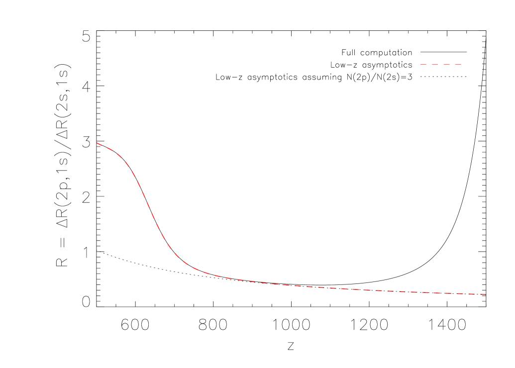
Fig. 4. Ratio of the net rates $\Delta R(2p,1s)$ to $\Delta R(2s,1s)$ for hydrogenic transitions. For comparison, we also show as dashed-line the approximate asymptotic behaviour of this ratio as given by equation 4. The deviations from statistical equilibrium of the relative populations of the 2p and 2s levels are important to accurately compute the low redshift behaviour of this function (see text for details).

Fig. 5. Ratio of the populations of levels $N(2p)$ and $N(2s)$, as derived from the numerical code of RCS06. At low redshifts, this ratio strongly deviates from the statistical equilibrium ratio of 3:1 (horizontal dotted line).

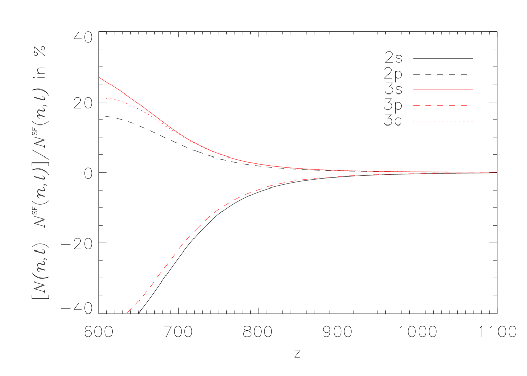
Fig. 6. Non-equilibrium effects on the populations of the angular momentum substates for levels $n=2$ and $n=3$. We present the ratio $N(n,l)/N^{\rm SE}(n,l)$, where the SE index refers to the statistical equilibrium population, and is computed from the actual total population of the shell using $N^{\rm SE}(n,l)=[(2l+1)/n^{2}]N_{tot}(n)$.

Fig. 1: Fractional net rates for the two transitions from levels $n=2$ to the ground state, computed using eq. 3. Around the peak of the Thomson visibility function, the $\Delta R(2s,1s)$ rate roughly contributes to $\sim 2/3$ of the total rate, while the Lyman-$\alpha$ route takes the other $\sim 1/3$. At higher redshifts, the Lyman-$\alpha$ route is the dominant recombinational channel. At redshifts below $z\sim 700$, this Lyman-$\alpha$ route becomes dominant again due to the higher statistical weight of the 2p level as compared to the 2s (ratio of 3 to 1).

Fig. 2: Redshift of formation for the Lyman-$\alpha$ and H-$\alpha$ lines. We present the normalised intensity for both transitions as a function of redshift z. For comparison, we also show the Thomson visibility function normalised to unity at the peak, showing that the redshift of formation of the recombinational lines is higher than that of formation of the CMB fluctuations. The low frequency wing of the Lyman-$\alpha$ line is significantly suppressed due to increasing role of 2s two photon decay. This is the main reason of the difference in the position of the maxima of the Lyman-$\alpha$ and H-$\alpha$ lines. Figure based from RCS06.

Fig. 3: Net rates for hydrogenic transitions from levels $n=2$ to the ground state. The rate $\Delta R(2p,1s)$ mimics the shape of the Ly$\alpha$ line (to be compared with Fig. 9 in RCS06). Note that the 2s two-photon decay rate dominates for redshifts between $z\sim 700$ to $\sim 1400$, where the bulk of recombination is taking place.

Fig. 4: Ratio of the net rates $\Delta R(2p,1s)$ to $\Delta R(2s,1s)$ for hydrogenic transitions. For comparison, we also show as dashed-line the approximate asymptotic behaviour of this ratio as given by equation 4. The deviations from statistical equilibrium of the relative populations of the 2p and 2s levels are important to accurately compute the low redshift behaviour of this function (see text for details).

Fig. 5: Ratio of the populations of levels $N(2p)$ and $N(2s)$, as derived from the numerical code of RCS06. At low redshifts, this ratio strongly deviates from the statistical equilibrium ratio of 3:1 (horizontal dotted line).

Fig. 6: Non-equilibrium effects on the populations of the angular momentum substates for levels $n=2$ and $n=3$. We present the ratio $N(n,l)/N^{\rm SE}(n,l)$, where the SE index refers to the statistical equilibrium population, and is computed from the actual total population of the shell using $N^{\rm SE}(n,l)=[(2l+1)/n^{2}]N_{tot}(n)$.