A Fast and Robust TSVM for Pattern Classification

Bin-Bin Gao csgaobb@gmail.com Jian-Jun Wang wjj@swu.edu.cn YouTu Lab, Tencent, Shenzhen 518000, China. School of Mathematics and Statistics, Southwest University, Chongqing 400715, China.
Abstract

Twin support vector machine (TSVM) is a powerful learning algorithm by solving a pair of small-sized SVM-type problems. However, there are still some specific issues such as low efficiency and weak robustness when it is faced with some applications. In this paper, we propose a Fast and Robust TSVM (FR-TSVM) to deal with the above issues. In order to strengthen model robustness, we propose an effective fuzzy membership function and reformulate the TSVMs such that different input instances can make different contributions to the learning of the decision hyperplane. To further speed up the training procedure, we develop an efficient coordinate descent algorithm with shirking to solve the involved a pair of quadratic programming problems (QPPs). Moreover, the theoretical foundations of the proposed approach are analyzed in details. The experimental results on several artificial and benchmark datasets indicate that the FR-TSVM not only obtains a fast learning speed but also shows a robust classification performance. Code has been made available at: https://github.com/gaobb/FR-TSVM.

keywords:
Pattern classification , Support vector machine, Twin support vector machine , Fuzzy membership , Coordinate descent method

1 Introduction

Support vector machine (SVM), invented by Vapnik [1], is a very popular machine learning algorithm. Due to the adoption structural risk minimization principle, SVM is capable of handling excellently with many classification and regression problems, such as machine fault-diagnosis [2], image identification [3], text classification [4], biomedicine [5] and financial forecast [6], etc. It has become a prominent highlight of machine learning research. However, the application of SVM is occasionally restricted by some practical issues, especially computational speed and model robustness. To overcome these limitations, some solutions have also been proposed.

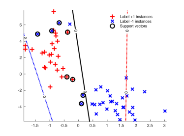
Mangasarian et al. [7] changed the proximal planes which are originally parallel to each other to generate a maximal spaced separating hyperplane into nonparallel ones, and proposed a generalized eigenvalue proximal SVM (GEPSVM). The GEPSVM speed-ups training with slighter accurate performance since it is solved by a pair of simple generalized eigenvalue problems. Following this concept, Jayadeva et al[8] proposed twin SVM (TSVM). Its objective is turned to be optimized by placing the non-parallel proximal planes as closely as possible to their corresponding instances’ cluster and as far as possible from their adversary instances’ cluster (as shown in Fig. 1a). Therefore, the TSVM algorithm converts GEPSVM into a pair of SVM-like convex programs and computation time is reduced satisfactorily to one-fourth of that of a conventional SVM. Recently, numerous nonparallel proximal-plane learning methods are proposed as variants of TSVM, such as TBSVM [9], Structural TSVM [10], Robust TSVM [11], Laplacian Smooth TSVM [12], Least-square TSVM(Ls-TSVM) [13], Ls-TSVM for multi-class [14], Twin Parametric-margin SVM [15, 16], Multi-label TSVM [17], RPTWSVM [18] and Pin-TSVM [19]. In additional, some regression model based TSVM are also proposed such as TSVR [20],  TPSVR[21], ϵitalic-ϵ\epsilon-TSVR [22], TWSVR [23] and v𝑣v-TWSVR [24]. All of the proposed variants share the same merits of TSVM. However, one challenge is that training instances from real-world applications often carry information with significant noise. These TSVM methods are sensitive to outliers or noises.

Noisy data often can deteriorate the generalization ability of SVM or TSVM. In term of fuzzy theory technique, noisy information can be causally converted into the fuzzy information to meet fuzzy inference theory. The training of SVM would be too sensitive to noisy inputs if all training instances are treated equivalently at the training stage. A conceptual way to alleviate this sensitive deterioration is to contract the influence of noisy inputs. This means that a conventional SVM, which intrinsically treats every input instance in equivalence, can be improved by introducing fuzzy membership functions to soften input information. A category of fuzzy SVMs are hence developed, such as Lin and Wang [25, 26], Wu and Liu [27], Inoue and Abe [28], Yang et al. [29], and Tang [30] etc. The elementary concept of fuzzy SVM is to allocate a small confident membership for each noisy instance consistent with the information fuzziness which the instance has carried to reduce its influence on the optimization. The membership is generally assigned according to the instance’s confidence intrinsically related to its native class. The introduction of fuzzy membership reduces effectively the uncertainty caused by noisy instances and leads to a robust classifier. To utilize the fuzzy concept, some variants of fuzzy TSVM have been developed in [31, 32, 33]. However, these fuzzy SVM methods equivalently assigned the fuzzy membership to each instance and they cannot distinguish support vectors and outliers effectively.

In term of computational efficiency, plenty of input instances from real-world applications require abundant quadratic programming computations, which slow down training efficiency. This computational cost significantly limits the applications of SVM. There are various solutions for improvement, including chunking [34], decomposition [35], sequential minimal optimization (SMO) [36] etc. However, they need to optimize the entire set of nonzero Lagrangian multipliers and the generated kernel matrix may still be too large to adapt to memory. Recently, Chang et al. proposed a primal coordinate descent (CD) method to deal with large-scale linear SVM [37, 38, 39].

In this paper, we propose a fast and robust twin support vector machine (FR-TSVM) for a classification problem. Our contributions are summarized as follows.

  • \bullet

    We construct a novel fuzzy membership function to measure the importance of each training instance. The assignment policy of fuzzy membership depends on the structural information of training instances in feature space.

  • \bullet

    We embed the proposed fuzzy concept into TSVM and propose a fast and robust TSVM model. In FR-TSVM, different input instances can make different contributions to the learning of decision hyperplanes. The pro- posed model can effectively alleviate the effect of noisy instances and obtain a robust performance.

  • \bullet

    We develop further coordinate descent algorithm with shrinking to speed-up the computations of linear and nonlinear FR-TSVM. In addition, this paper presents FR-TSVM in details including corresponding theoretical fundamentals and related properties.

  • \bullet

    Experiments on artificial and benchmark datasets show that the proposal brings more satisfactory performances on both classification accuracy and learning efficiency, compared with traditional SVM, FSVM and TSVM.

The remaining parts of this paper are organized as follows. We first briefly review the basics of classical SVM and its related works, including FSVM and TSVM in Section 2. Then, Section 3 proposes FR-TSVM approach, including fuzzy membership function construction, linear and nonlinear FR-TSVM models and their optimization algorithms. After that, experimental results are reported in Section 4. Some preliminary results have been published in a conference presentation [40].
Refer to caption
(a) TSVM
Refer to caption
(b) FR-TSVM
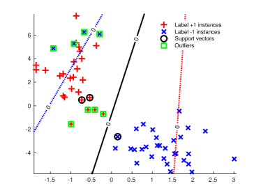
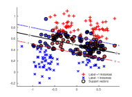
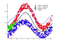
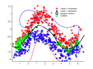
Figure 1: Geometric interpretation of linear TSVM and FR-TSVM for binary classification. Red “ +” and blue “ x” represent positive and negative instances, respectively. A pair of nonparallel decision hyperplanes are shown by red and blue dashed line and the best decision plane is represented by a black line. We can see that the proposed method is easy to get a better decision hyperplane because it can effectively detect noisy points and weaken their effects.

2 Background

In this paper, we mainly focus on a binary classification problem in the n𝑛n-dimensional space nsuperscript𝑛\mathcal{R}^{n}. We denote training data as D={(xi,yi)|i=1,2,,l}𝐷conditional-setsubscript𝑥𝑖subscript𝑦𝑖𝑖12𝑙D=\{(\vec{x}_{i},y_{i})|i=1,2,\dotsc,l\}, where xinsubscript𝑥𝑖superscript𝑛\vec{x}_{i}\in\mathcal{R}^{n} represents an input instance with the corresponding label yi{+1,1}subscript𝑦𝑖11y_{i}\in\{+1,-1\}. Without loss of generality, we assume that the matrix X𝑋X with size of l×n𝑙𝑛l\times n represents all training instances, and the matrices X±subscript𝑋plus-or-minusX_{\pm} with sizes of l±×nsubscript𝑙plus-or-minus𝑛l_{\pm}\times n represent the training instances belonging to “+1”(positive) or “-1”(negative) class, respectively, where l=l++l𝑙subscript𝑙subscript𝑙l=l_{+}+l_{-}.

2.1 Support vector machine

As a classical machine learning algorithm, the standard linear SVM [1] aims to construct a pair of parallel hyperplanes between two classes of instances:

wTx+b=+1andwTx+b=1,superscript𝑤T𝑥𝑏1andsuperscript𝑤T𝑥𝑏1\vec{w}^{\rm T}\vec{x}+b=+1\leavevmode\nobreak\ \textrm{and}\leavevmode\nobreak\ \vec{w}^{\rm T}\vec{x}+b=-1\,, (1)

where wn𝑤superscript𝑛\vec{w}\in\mathcal{R}^{n} and b𝑏b\in\mathcal{R} are the normal vector and the bias term of hyperplanes, respectively. These separating hyperplanes are obtained by solving the following quadratic programming problem (QPP):

minw,b,ξi12w2+ci=1lξis.t.yi(wTxi+b)+ξi1,ξi0,i=1,2,,l.formulae-sequencesubscript𝑤𝑏subscript𝜉𝑖12superscriptdelimited-∥∥𝑤2𝑐superscriptsubscript𝑖1𝑙subscript𝜉𝑖s.t.subscript𝑦𝑖superscript𝑤𝑇subscript𝑥𝑖𝑏subscript𝜉𝑖1formulae-sequencesubscript𝜉𝑖0𝑖12𝑙\displaystyle\begin{split}&\min_{\vec{w},b,\xi_{i}}\leavevmode\nobreak\ \frac{1}{2}{\|\vec{w}\|}^{2}+c\sum_{i=1}^{l}\xi_{i}\\ &\textrm{s.t.}\leavevmode\nobreak\ \leavevmode\nobreak\ y_{i}(\vec{w}^{T}\vec{x}_{i}+b)+\xi_{i}\geq 1,\xi_{i}\geq\vec{0},i=1,2,\dotsc,l.\end{split} (2)

where .\|.\| stands for 2subscript2\ell_{2}-norm, ξisubscript𝜉𝑖\xi_{i} is called as slack variable which denotes the misclassification error associated with the i𝑖i-th input instance and c>0𝑐0c>0 is regularization factor that balances the importance between the maximization of margin width (i.e., the minimization of 12w212superscriptnorm𝑤2\frac{1}{2}{\|\vec{w}\|}^{2}) and the minimization of the training error. The dual QPP of problem Eq.(2) is:

maxαi=1lαi+12i=1lj=1lyiyjxi,xjαiαjs.t.i=1lαiyi=0,0αi1,i=1,2,,l,formulae-sequencesubscript𝛼superscriptsubscript𝑖1𝑙subscript𝛼𝑖12superscriptsubscript𝑖1𝑙superscriptsubscript𝑗1𝑙subscript𝑦𝑖subscript𝑦𝑗subscript𝑥𝑖subscript𝑥𝑗subscript𝛼𝑖subscript𝛼𝑗s.t.superscriptsubscript𝑖1𝑙subscript𝛼𝑖subscript𝑦𝑖00subscript𝛼𝑖1𝑖12𝑙\displaystyle\begin{split}&\max_{\vec{\alpha}}\leavevmode\nobreak\ \sum_{i=1}^{l}\alpha_{i}+\frac{1}{2}\sum_{i=1}^{l}\sum_{j=1}^{l}y_{i}y_{j}\langle\vec{x}_{i},\vec{x}_{j}\rangle\alpha_{i}\alpha_{j}\\ &\textrm{s.t.}\leavevmode\nobreak\ \leavevmode\nobreak\ \sum_{i=1}^{l}\alpha_{i}y_{i}=0,0\leq\alpha_{i}\leq 1,i=1,2,\dotsc,l\,,\end{split} (3)

where αl𝛼superscript𝑙\vec{\alpha}\in\mathcal{R}^{l} is Lagrangian multiplier. After solving this dual QPP, a testing instance x𝑥\vec{x} is classified as “+1” or “-1” following decision function

f(x)=sign(wTx+b)𝑓𝑥signsuperscript𝑤absentT𝑥superscript𝑏f(\vec{x})=\operatorname*{sign}(\vec{w}^{*\rm T}\vec{x}+b^{*}) (4)

where (w,b)superscript𝑤superscript𝑏(\vec{w}^{*},b^{*}) and αisubscriptsuperscript𝛼𝑖\alpha^{*}_{i} are the solution of Eq.(2) and Eq.(3), respectively.

2.2 Twin support vector machine

Different from the conventional SVM, TSVM is in fact constructed by two non-parallel decision planes, i.e.,

w+Tx+b+=0andwTx+b=0.superscriptsubscript𝑤T𝑥subscript𝑏0andsuperscriptsubscript𝑤T𝑥subscript𝑏0\vec{w}_{+}^{\rm T}\vec{x}+b_{+}=0\leavevmode\nobreak\ \textrm{and}\leavevmode\nobreak\ \vec{w}_{-}^{\rm T}\vec{x}+b_{-}=0\,. (5)

To construct such two non-parallel decision planes, a pair of primal optimization problems are set up:

minw+,b+,ξ12X+w++e+b+2+c1eTξs.t.(Xw++eb+)+ξe,ξ0,formulae-sequencesubscriptsubscript𝑤subscript𝑏subscript𝜉12superscriptdelimited-∥∥subscript𝑋subscript𝑤subscript𝑒subscript𝑏2subscript𝑐1superscriptsubscript𝑒Tsubscript𝜉s.t.subscript𝑋subscript𝑤subscript𝑒subscript𝑏subscript𝜉subscript𝑒subscript𝜉0\begin{split}&\min_{\vec{w}_{+},b_{+},\vec{\xi}_{-}}\leavevmode\nobreak\ \leavevmode\nobreak\ \leavevmode\nobreak\ \frac{1}{2}\parallel X_{+}\vec{w}_{+}+\vec{e}_{+}b_{+}\parallel^{2}+c_{1}\vec{e}_{-}^{\rm T}\vec{\xi}_{-}\\ &\textrm{s.t.}\leavevmode\nobreak\ \leavevmode\nobreak\ -(X_{-}\vec{w}_{+}+\vec{e}_{-}b_{+})+\vec{\xi}_{-}\geq\vec{e}_{-},\vec{\xi}_{-}\geq\vec{0}\,,\\ \end{split} (6)

and

minw,b,ξ+12Xw+eb2+c2e+Tξ+s.t.(X+w+e+b)+ξ+e+,ξ+0,formulae-sequencesubscriptsubscript𝑤subscript𝑏subscript𝜉12superscriptdelimited-∥∥subscript𝑋subscript𝑤subscript𝑒subscript𝑏2subscript𝑐2superscriptsubscript𝑒Tsubscript𝜉s.t.subscript𝑋subscript𝑤subscript𝑒subscript𝑏subscript𝜉subscript𝑒subscript𝜉0\begin{split}&\min_{\vec{w}_{-},b_{-},\vec{\xi}_{+}}\leavevmode\nobreak\ \leavevmode\nobreak\ \leavevmode\nobreak\ \frac{1}{2}\parallel X_{-}\vec{w}_{-}+\vec{e}_{-}b_{-}\parallel^{2}+c_{2}\vec{e}_{+}^{\rm T}\vec{\xi}_{+}\\ &\textrm{s.t.}\leavevmode\nobreak\ \leavevmode\nobreak\ \leavevmode\nobreak\ (X_{+}\vec{w}_{-}+\vec{e}_{+}b_{-})+\vec{\xi}_{+}\geq\vec{e}_{+},\vec{\xi}_{+}\geq\vec{0}\,,\end{split} (7)

where c1>0subscript𝑐10c_{1}>0 and c2>0subscript𝑐20c_{2}>0 are parameters, ξ+subscript𝜉\vec{\xi}_{+} and ξsubscript𝜉\vec{\xi}_{-} denote the vectors of slack variables for positive and negative classes, respectively, and e+,esubscript𝑒subscript𝑒\vec{e}_{+},\vec{e}_{-} correspond to unit vectors with l±subscript𝑙plus-or-minusl_{\pm} dimensions. By introducing the Lagrangian multipliers, the dual QPPs of Eq.(6) and Eq.(7) can be represented as followings

maxαeTα12αTH(H+TH+)1HTαs.t.0αc1e,subscript𝛼superscriptsubscript𝑒T𝛼12superscript𝛼Tsubscript𝐻superscriptsuperscriptsubscript𝐻Tsubscript𝐻1superscriptsubscript𝐻T𝛼s.t.0𝛼subscript𝑐1subscript𝑒\begin{split}&\max_{\vec{\alpha}}\quad\vec{e}_{-}^{\rm T}\vec{\alpha}-\frac{1}{2}\vec{\alpha}^{\rm T}H_{-}(H_{+}^{\rm T}H_{+})^{-1}H_{-}^{\rm T}\vec{\alpha}\\ &\textrm{s.t.}\quad\vec{0}\leq\vec{\alpha}\leq c_{1}\vec{e}_{-},\end{split} (8)
maxβe+Tβ12βTH+(HTH)1H+Tβs.t.0βc2e+,subscript𝛽superscriptsubscript𝑒T𝛽12superscript𝛽Tsubscript𝐻superscriptsuperscriptsubscript𝐻Tsubscript𝐻1superscriptsubscript𝐻T𝛽s.t.0𝛽subscript𝑐2subscript𝑒\begin{split}&\max_{\vec{\beta}}\quad\vec{e}_{+}^{\rm T}\vec{\beta}-\frac{1}{2}\vec{\beta}^{\rm T}H_{+}(H_{-}^{\rm T}H_{-})^{-1}H_{+}^{\rm T}\vec{\beta}\\ &\textrm{s.t.}\quad\vec{0}\leq\vec{\beta}\leq c_{2}\vec{e}_{+},\end{split} (9)

where H+=[X+,e+],H=[X,e]formulae-sequencesubscript𝐻subscript𝑋subscript𝑒subscript𝐻subscript𝑋subscript𝑒H_{+}=[X_{+},\vec{e}_{+}],H_{-}=[X_{-},\vec{e}_{-}]. The non-parallel hyperplanes Eq.(5) can be obtained from the solutions αsuperscript𝛼\vec{\alpha}^{*} and βsuperscript𝛽\vec{\beta}^{*} of Eq.(LABEL:eq:d-tsvm1) and Eq.(LABEL:eq:d-tsvm2) by

u+=(H+TH+)1HT𝜶,u=(HTH)1H+T𝜷,formulae-sequencesuperscriptsubscript𝑢superscriptsuperscriptsubscript𝐻Tsubscript𝐻1superscriptsubscript𝐻Tsuperscript𝜶superscriptsubscript𝑢superscriptsuperscriptsubscript𝐻Tsubscript𝐻1superscriptsubscript𝐻Tsuperscript𝜷\vec{u}_{+}^{*}=-(H_{+}^{\rm T}H_{+})^{-1}H_{-}^{\rm T}\boldsymbol{\alpha}^{*},\vec{u}_{-}^{*}=(H_{-}^{\rm T}H_{-})^{-1}H_{+}^{\rm T}\boldsymbol{\beta}^{*}, (10)

where u±=[w±T,b±]Tsuperscriptsubscript𝑢plus-or-minussuperscriptsuperscriptsubscript𝑤plus-or-minusabsentTsuperscriptsubscript𝑏plus-or-minusT\vec{u}_{\pm}^{*}=[\vec{w}_{\pm}^{*\rm T},b_{\pm}^{*}]^{\rm T}, w±Tsuperscriptsubscript𝑤plus-or-minusabsentTw_{\pm}^{*\rm T} and b±superscriptsubscript𝑏plus-or-minusb_{\pm}^{*} are the solutions of Eq.(6) and Eq.(7). TSVM then can easily assign a label “+1” or “-1” to a testing instance x𝑥\vec{x} by

f(x)=argmin±w±Tx+b±w±,𝑓𝑥subscriptargminplus-or-minusdelimited-∣∣superscriptsubscriptsuperscript𝑤plus-or-minusT𝑥subscriptsuperscript𝑏plus-or-minusnormsubscriptsuperscript𝑤plus-or-minusf(\vec{x})=\operatorname*{argmin}_{\pm}\frac{\mid{\vec{w}^{*}_{\pm}}^{\rm T}\vec{x}+b^{*}_{\pm}\mid}{\parallel\vec{w}^{*}_{\pm}\parallel}\,, (11)

where |||\cdot| is a function taking its absolute value. If the matrix H+TH+superscriptsubscript𝐻Tsubscript𝐻H_{+}^{\rm T}H_{+} or HTHsuperscriptsubscript𝐻Tsubscript𝐻H_{-}^{\rm T}H_{-} is ill-conditioned, TSVM artificially introduces a term λI(λ>0)𝜆𝐼𝜆0\lambda I(\lambda>0), where I𝐼I is an identity matrix of appropriate dimension. In the experiments, we fix the value of λ𝜆\lambda as 0.01.

2.3 Fuzzy support vector machine

To reduce the effects of outliers, Lin et al. introduced fuzzy membership to each input instance of SVM and proposed fuzzy SVM (FSVM) [25]. In FSVM, training instance xisubscript𝑥𝑖\vec{x}_{i} is assigned a fuzzy membership 0si10subscript𝑠𝑖10\leq s_{i}\leq 1 besides a label yi{+1,1}subscript𝑦𝑖11y_{i}\in\{+1,-1\}. The input dataset T𝑇T is thus modified as T={(xi,yi,si)|i=1,2,,l}superscript𝑇conditional-setsubscript𝑥𝑖subscript𝑦𝑖subscript𝑠𝑖𝑖12𝑙T^{\prime}=\{(\vec{x}_{i},y_{i},s_{i})|i=1,2,\dotsc,l\}. These fuzzy memberships {si|i=1,2,,l}conditional-setsubscript𝑠𝑖𝑖12𝑙\{s_{i}|i=1,2,\dotsc,l\} are used to reduce the influence of noisy instances for generating final decision function, which induces fuzzy SVM as followings:

minw,b,ξ12w2+ci=1lsiξis.t.yi(wTxi+b)+ξi1,ξi0,i=1,2,,l.formulae-sequencesubscript𝑤𝑏𝜉12superscriptdelimited-∥∥𝑤2𝑐superscriptsubscript𝑖1𝑙subscript𝑠𝑖subscript𝜉𝑖s.t.subscript𝑦𝑖superscript𝑤𝑇subscript𝑥𝑖𝑏subscript𝜉𝑖1formulae-sequencesubscript𝜉𝑖0𝑖12𝑙\displaystyle\begin{split}&\min_{\vec{w},b,\xi}\leavevmode\nobreak\ \frac{1}{2}{\|\vec{w}\|}^{2}+c\sum_{i=1}^{l}s_{i}\xi_{i}\\ &\textrm{s.t.}\leavevmode\nobreak\ \leavevmode\nobreak\ y_{i}(\vec{w}^{T}\vec{x}_{i}+b)+\xi_{i}\geq 1,\xi_{i}\geq 0,i=1,2,\dotsc,l.\end{split} (12)

It is noted that a smaller sisubscript𝑠𝑖s_{i} can reduce the effect of the parameter ξisubscript𝜉𝑖\xi_{i} in problem Eq.(12) so that the corresponding instance xisubscript𝑥𝑖\vec{x}_{i} can be treated as less important. The classification of any testing instance x𝑥\vec{x} can be obtained by determining the sign of wTx+bsuperscriptsuperscript𝑤T𝑥superscript𝑏{\vec{w}^{*}}^{\rm T}{\vec{x}}+b^{*} where wsuperscript𝑤\vec{w}^{*} and bsuperscript𝑏b^{*} are the solution of Eq.(12).

3 The proposed FR-TSVM approach

In this section, we will propose the approach of FR-TSVM. To this end, we first introduce fuzzy membership construction. Then, we propose linear and nonlinear FR-TSVM models by embedding fuzzy membership into TSVM. Finally, a fast optimization method is developed for solving the dual problems of the proposed FR-TSVM.

3.1 Fuzzy membership construction
Refer to caption
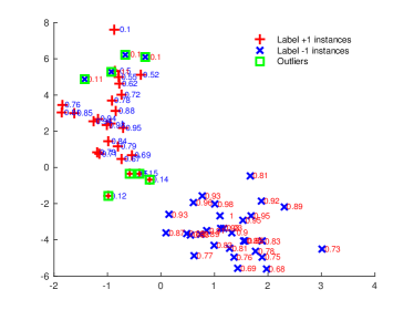
Figure 2: Linear fuzzy membership values for binary classification. The red and blue color numbers are fuzzy membership values for negative and positive instances, respectively. Fuzzy membership values of instances which close to class center are always larger.

Fuzzy membership plays a key role in robust classification learning. However, there is no unified standard to construct such fuzzy membership so far. As we know, support vectors geometrically locate near the boundary area of two adjacent classes. The noisy points also reside in this area typically and unfortunately. This means that support vectors and noisy points are frequently mixed together. Inspired by Tang [30], we propose a fuzzy membership assignment for training instances. The proposed method considers not only reducing the noise carried by the outliers but also keeping the importance of support vectors.

3.1.1 Linear case

The construction of fuzzy membership considers firstly linear kernel case. we define directly positive and negative class centers, xc+subscript𝑥limit-from𝑐\vec{x}_{c+} and xcsubscript𝑥limit-from𝑐\vec{x}_{c-}, as the mean points in the input space for positive and negative instances,

xc+=1l+yi=+1xi,xc=1lyi=1xi.formulae-sequencesubscript𝑥limit-from𝑐1subscript𝑙subscriptsubscript𝑦𝑖1subscript𝑥𝑖subscript𝑥limit-from𝑐1subscript𝑙subscriptsubscript𝑦𝑖1subscript𝑥𝑖\vec{x}_{c+}=\frac{1}{l_{+}}\sum_{y_{i}=+1}\vec{x}_{i}\,,\vec{x}_{c-}=\frac{1}{l_{-}}\sum_{y_{i}=-1}\vec{x}_{i}\,. (13)

Measuring the distance between instances and their class center, the hypersphere radius of positive and negative are defined and given as

r+=max{xixc+|yi=+1},subscript𝑟conditionalnormsubscript𝑥𝑖subscript𝑥limit-from𝑐subscript𝑦𝑖1r_{+}=\max\{\parallel\vec{x}_{i}-\vec{x}_{c+}\parallel|y_{i}=+1\}\,, (14)
r=max{xixc|yi=1}.subscript𝑟conditionalnormsubscript𝑥𝑖subscript𝑥limit-from𝑐subscript𝑦𝑖1r_{-}=\max\{\parallel\vec{x}_{i}-\vec{x}_{c-}\parallel|y_{i}=-1\}\,. (15)

With known xc+,xcsubscript𝑥limit-from𝑐subscript𝑥limit-from𝑐\vec{x}_{c+},\vec{x}_{c-}, r+subscript𝑟r_{+}, and rsubscript𝑟r_{-}, membership sisubscript𝑠𝑖s_{i} of an instance can be assigned according to the relationship between xixc+normsubscript𝑥𝑖subscript𝑥limit-from𝑐\parallel\vec{x}_{i}-\vec{x}_{c+}\parallel and xixcnormsubscript𝑥𝑖subscript𝑥limit-from𝑐\parallel\vec{x}_{i}-\vec{x}_{c-}\parallel. In this paper, sisubscript𝑠𝑖s_{i} of a positive instance be given as:

si={μ(1xixc+/(r++δ)),ifxixc+xixc&yi=+1(1μ)(1xixc+/(r++δ)),ifxixc+<xixc&yi=+1subscript𝑠𝑖cases𝜇1normsubscript𝑥𝑖subscript𝑥limit-from𝑐subscript𝑟𝛿missing-subexpressionmissing-subexpressionmissing-subexpressionifnormsubscript𝑥𝑖subscript𝑥limit-from𝑐normsubscript𝑥𝑖subscript𝑥limit-from𝑐subscript𝑦𝑖1missing-subexpressionmissing-subexpressionmissing-subexpression1𝜇1normsubscript𝑥𝑖subscript𝑥limit-from𝑐subscript𝑟𝛿missing-subexpressionmissing-subexpressionmissing-subexpressionifnormsubscript𝑥𝑖subscript𝑥limit-from𝑐normsubscript𝑥𝑖subscript𝑥limit-from𝑐subscript𝑦𝑖1missing-subexpressionmissing-subexpressionmissing-subexpressions_{i}=\left\{\begin{array}[]{llll}\mu\big{(}1-{\parallel\vec{x}_{i}-\vec{x}_{c+}\parallel}/({r_{+}+\delta)}\big{)},\\ \quad\textrm{if}\parallel\vec{x}_{i}-\vec{x}_{c+}\parallel\geq\parallel\vec{x}_{i}-\vec{x}_{c-}\parallel\&\leavevmode\nobreak\ y_{i}=+1\\ \big{(}1-\mu\big{)}\big{(}1-{\parallel\vec{x}_{i}-\vec{x}_{c+}\parallel}/({r_{+}+\delta)}\big{)},\\ \quad\textrm{if}\parallel\vec{x}_{i}-\vec{x}_{c+}\parallel<\parallel\vec{x}_{i}-\vec{x}_{c-}\parallel\&\leavevmode\nobreak\ y_{i}=+1\end{array}\right. (16)

where μ[0,1]𝜇01\mu\in[0,1] is used to balance the effect of normal and noisy instances, and δ>0𝛿0\delta>0 to avoid si=0subscript𝑠𝑖0s_{i}=0. The relationship reveals that an instance is generally assigned by a proportionally decreasing sisubscript𝑠𝑖s_{i} value when it drifts farther from its native class center to increase uncertainty. Moreover, some instances are highly suspected as outliers which dwell with a sufficient far distance from their native class center(i.e. xixc+xixcnormsubscript𝑥𝑖subscript𝑥limit-from𝑐normsubscript𝑥𝑖subscript𝑥limit-from𝑐\parallel\vec{x}_{i}-\vec{x}_{c+}\parallel\geq\parallel\vec{x}_{i}-\vec{x}_{c-}\parallel). In order to decrease outliers’ effect toward the hyperplane, we assign a small positive real number for μ𝜇\mu. In practice, we set u=0.1𝑢0.1u=0.1 for FR-TSVM. A similar rule can be applied to the fuzzy membership of those negative instances. As shown in Fig. 2, we intuitively show linear fuzzy membership values for training instances.

3.1.2 Nonlinear case

For nonlinear case, fuzzy membership function must be consistently reconstructed in the feature space \mathcal{H}. Similar to linear case, positive and negative class centers φc+subscript𝜑limit-from𝑐\vec{\varphi}_{c+} and φcsubscript𝜑limit-from𝑐\vec{\varphi}_{c-} in the feature space are defined as:

φc+=1l+yi=+1φ(xi),φc=1lyi=1φ(xi).formulae-sequencesubscript𝜑limit-from𝑐1subscript𝑙subscriptsubscript𝑦𝑖1𝜑subscript𝑥𝑖subscript𝜑limit-from𝑐1subscript𝑙subscriptsubscript𝑦𝑖1𝜑subscript𝑥𝑖\vec{\varphi}_{c+}=\frac{1}{l_{+}}\sum_{\mathclap{y_{i}=+1}}\varphi(\vec{x}_{i})\,,\vec{\varphi}_{c-}=\frac{1}{l_{-}}\sum_{\mathclap{y_{i}=-1}}\varphi(\vec{x}_{i})\,. (17)

where φ(xi)𝜑subscript𝑥𝑖\varphi(\vec{x}_{i})\in\mathcal{H} denotes the transformation of an arbitrary input instance xisubscript𝑥𝑖\vec{x}_{i}. The squared distance from φ(xi)𝜑subscript𝑥𝑖\varphi(\vec{x}_{i}) to φc+subscript𝜑limit-from𝑐\vec{\varphi}_{c+} or φcsubscript𝜑limit-from𝑐\vec{\varphi}_{c-} can be rearranged and expressed in terms of the kernel function κ(,)𝜅\kappa(\cdot,\cdot):

φ(xi)φc+2superscriptnorm𝜑subscript𝑥𝑖subscript𝜑limit-from𝑐2\displaystyle{\parallel\varphi(\vec{x}_{i})-\vec{\varphi}_{c+}\parallel}^{2}
=φ(xi)22φ(xi),φc++φc+2absentsuperscriptnorm𝜑subscript𝑥𝑖22𝜑subscript𝑥𝑖subscript𝜑limit-from𝑐superscriptnormsubscript𝜑limit-from𝑐2\displaystyle\hskip 11.38109pt={\|\varphi(\vec{x}_{i})\|^{2}-2\langle\varphi(\vec{x}_{i}),\vec{\varphi}_{c+}\rangle+\|\vec{\varphi}_{c+}\|^{2}}
=φ(xi),φ(xi)2l+yj=+1φ(xi),φ(xj)absent𝜑subscript𝑥𝑖𝜑subscript𝑥𝑖2subscript𝑙subscriptsubscript𝑦𝑗1𝜑subscript𝑥𝑖𝜑subscript𝑥𝑗\displaystyle\hskip 11.38109pt=\langle\varphi(\vec{x}_{i}),\varphi(\vec{x}_{i})\rangle-\frac{2}{l_{+}}\sum_{\mathclap{y_{j}=+1}}\langle\varphi(\vec{x}_{i}),\varphi(\vec{x}_{j})\rangle
+1l+2yi=+1yk=+1φ(xi),φ(xk)1superscriptsubscript𝑙2subscriptsubscript𝑦𝑖1subscriptsubscript𝑦𝑘1𝜑subscript𝑥𝑖𝜑subscript𝑥𝑘\displaystyle\hskip 22.76219pt+\frac{1}{l_{+}^{2}}\sum_{{y_{i}=+1}}\sum_{y_{k}=+1}\langle\varphi(\vec{x}_{i}),\varphi(\vec{x}_{k})\rangle
=κ(xi,xi)2l+yj=+1κ(xi,xj)absent𝜅subscript𝑥𝑖subscript𝑥𝑖2subscript𝑙subscriptsubscript𝑦𝑗1𝜅subscript𝑥𝑖subscript𝑥𝑗\displaystyle\hskip 11.38109pt=\kappa(\vec{x}_{i},\vec{x}_{i})-\frac{2}{l_{+}}\sum_{\mathclap{y_{j}=+1}}\kappa(\vec{x}_{i},\vec{x}_{j})
+1l+2yi=+1yk=+1κ(xi,xk),1superscriptsubscript𝑙2subscriptsubscript𝑦𝑖1subscriptsubscript𝑦𝑘1𝜅subscript𝑥𝑖subscript𝑥𝑘\displaystyle\hskip 22.76219pt+\frac{1}{l_{+}^{2}}\sum_{y_{i}=+1}\sum_{y_{k}=+1}\kappa(\vec{x}_{i},\vec{x}_{k}), (18)

and

φ(xi)φc2superscriptnorm𝜑subscript𝑥𝑖subscript𝜑limit-from𝑐2\displaystyle{\parallel\varphi(\vec{x}_{i})-\vec{\varphi}_{c-}\parallel}^{2}
=κ(xi,xi)2lyj=1κ(xi,xj)absent𝜅subscript𝑥𝑖subscript𝑥𝑖2subscript𝑙subscriptsubscript𝑦𝑗1𝜅subscript𝑥𝑖subscript𝑥𝑗\displaystyle\hskip 11.38109pt=\kappa(\vec{x}_{i},\vec{x}_{i})-\frac{2}{l_{-}}\sum_{\mathclap{y_{j}=-1}}\kappa(\vec{x}_{i},\vec{x}_{j})
+1l2yi=1yk=1κ(xi,xk),1superscriptsubscript𝑙2subscriptsubscript𝑦𝑖1subscriptsubscript𝑦𝑘1𝜅subscript𝑥𝑖subscript𝑥𝑘\displaystyle\hskip 22.76219pt+\frac{1}{l_{-}^{2}}\sum_{y_{i}=-1}\sum_{y_{k}=-1}\kappa(\vec{x}_{i},\vec{x}_{k}), (19)

where κ(xi.xj)\kappa(\vec{x}_{i}.\vec{x}_{j}) is the kernel function which implicitly calculates the high-dimensional dot-product of φ(xi)𝜑subscript𝑥𝑖\varphi(\vec{x}_{i}) and φ(xj)𝜑subscript𝑥𝑗\varphi(\vec{x}_{j}). The scattering hypersphere radii in the feature space are

rφ+=max{φ(xi)φc+|yi=+1},subscript𝑟limit-from𝜑conditionalnorm𝜑subscript𝑥𝑖subscript𝜑limit-from𝑐subscript𝑦𝑖1r_{\varphi+}=\max\{\parallel\varphi(\vec{x}_{i})-\vec{\varphi}_{c+}\parallel|y_{i}=+1\}\,, (20)
rφ=max{φ(xi)φc|yi=1}.subscript𝑟limit-from𝜑conditionalnorm𝜑subscript𝑥𝑖subscript𝜑limit-from𝑐subscript𝑦𝑖1r_{\varphi-}=\max\{\parallel\varphi(\vec{x}_{i})-\vec{\varphi}_{c-}\parallel|y_{i}=-1\}\,. (21)

Based on the same principle in linear case, the fuzzy membership function for non-linear kernel can equivalently given as:

si={μ(1φ(xi)φc+2/(rφ+2+δ) ),ifφ(xi)φc+φ(xi)φc&yi=+1(1μ)(1φ(xi)φc+2/(rφ+2+δ) ),ifφ(xi)φc+<φ(xi)φc&yi=+1subscript𝑠𝑖cases𝜇1φ(xi)φc+2/(rφ+2+δ) missing-subexpressionifnorm𝜑subscript𝑥𝑖subscript𝜑limit-from𝑐norm𝜑subscript𝑥𝑖subscript𝜑limit-from𝑐subscript𝑦𝑖1missing-subexpression1𝜇1φ(xi)φc+2/(rφ+2+δ) missing-subexpressionifnorm𝜑subscript𝑥𝑖subscript𝜑limit-from𝑐norm𝜑subscript𝑥𝑖subscript𝜑limit-from𝑐subscript𝑦𝑖1missing-subexpressions_{i}=\left\{\begin{array}[]{ll}\mu\big{(}1-\mathchoice{{\hbox{$\displaystyle\sqrt{{\parallel\varphi(\vec{x}_{i})-\vec{\varphi}_{c+}\parallel}^{2}/(r_{\varphi+}^{2}+\delta)\,}$}\lower 0.4pt\hbox{\vrule height=9.30444pt,depth=-7.44359pt}}}{{\hbox{$\textstyle\sqrt{{\parallel\varphi(\vec{x}_{i})-\vec{\varphi}_{c+}\parallel}^{2}/(r_{\varphi+}^{2}+\delta)\,}$}\lower 0.4pt\hbox{\vrule height=9.30444pt,depth=-7.44359pt}}}{{\hbox{$\scriptstyle\sqrt{{\parallel\varphi(\vec{x}_{i})-\vec{\varphi}_{c+}\parallel}^{2}/(r_{\varphi+}^{2}+\delta)\,}$}\lower 0.4pt\hbox{\vrule height=8.43332pt,depth=-6.74669pt}}}{{\hbox{$\scriptscriptstyle\sqrt{{\parallel\varphi(\vec{x}_{i})-\vec{\varphi}_{c+}\parallel}^{2}/(r_{\varphi+}^{2}+\delta)\,}$}\lower 0.4pt\hbox{\vrule height=8.43332pt,depth=-6.74669pt}}}\big{)},\\ \textrm{if}\leavevmode\nobreak\ \parallel\varphi(\vec{x}_{i})-\vec{\varphi}_{c+}\parallel\geq\parallel\varphi(\vec{x}_{i})-\vec{\varphi}_{c-}\parallel\&\leavevmode\nobreak\ y_{i}=+1\\ \big{(}1-\mu\big{)}\big{(}1-\mathchoice{{\hbox{$\displaystyle\sqrt{{\parallel\varphi(\vec{x}_{i})-\vec{\varphi}_{c+}\parallel}^{2}/(r_{\varphi+}^{2}+\delta)\,}$}\lower 0.4pt\hbox{\vrule height=9.30444pt,depth=-7.44359pt}}}{{\hbox{$\textstyle\sqrt{{\parallel\varphi(\vec{x}_{i})-\vec{\varphi}_{c+}\parallel}^{2}/(r_{\varphi+}^{2}+\delta)\,}$}\lower 0.4pt\hbox{\vrule height=9.30444pt,depth=-7.44359pt}}}{{\hbox{$\scriptstyle\sqrt{{\parallel\varphi(\vec{x}_{i})-\vec{\varphi}_{c+}\parallel}^{2}/(r_{\varphi+}^{2}+\delta)\,}$}\lower 0.4pt\hbox{\vrule height=8.43332pt,depth=-6.74669pt}}}{{\hbox{$\scriptscriptstyle\sqrt{{\parallel\varphi(\vec{x}_{i})-\vec{\varphi}_{c+}\parallel}^{2}/(r_{\varphi+}^{2}+\delta)\,}$}\lower 0.4pt\hbox{\vrule height=8.43332pt,depth=-6.74669pt}}}\big{)},\\ \textrm{if}\leavevmode\nobreak\ \parallel\varphi(\vec{x}_{i})-\vec{\varphi}_{c+}\parallel<\parallel\varphi(\vec{x}_{i})-\vec{\varphi}_{c-}\parallel\&\leavevmode\nobreak\ y_{i}=+1\end{array}\right. (22)

where δ𝛿\delta is similarly defined as a small positive constant to avoid the vanishing of sisubscript𝑠𝑖s_{i}. Of course, a fuzzy membership function sisubscript𝑠𝑖s_{i} for negative class instances can be similarly defined.

3.2 Fast and Robust twin support vector machine

In this section, we propose an efficient learning approach termed as fast and robust twin support vector machine (FR-TSVM). As mentioned earlier, the FR-MSVM is similar to TSVM, as it also derives a pair of nonparallel decision hyperplanes through two QPPs. What is more, FR-TSVM is more robust and fast than TSVM.

3.2.1 Linear FR-TSVM

For linear case, the FR-TSVM finds two nonparallel hyperplanes in nsuperscript𝑛\mathcal{R}^{n} space

w+Tx+b+=0,andwTx+b=0.formulae-sequencesuperscriptsubscript𝑤T𝑥subscript𝑏0𝑎𝑛𝑑superscriptsubscript𝑤T𝑥subscript𝑏0\vec{w}_{+}^{\rm T}\vec{x}+b_{+}=0,\quad and\quad\vec{w}_{-}^{\rm T}\vec{x}+b_{-}=0. (23)

Considering the crucial trade-off balance between margin maximization and error minimization, a margin term similar to that in the standard SVM [1], should be added firstly in the model. Since TSVM has two proximal decision functions, w±Tx+b±=0superscriptsubscript𝑤plus-or-minusT𝑥subscript𝑏plus-or-minus0\vec{w}_{\pm}^{\rm T}\vec{x}+b_{\pm}=0, two margin terms 1/w+1normsubscript𝑤1/\|\vec{w}_{+}\| and 1/w1normsubscript𝑤1/\|\vec{w}_{-}\| are accordingly defined for proximal decision functions, respectively. Together with the introduced fuzzy membership function and the margin terms, a weight regularized model of FR-TSVM with the linear kernel is hence proposed:

minw+,b+,ξ12c1w+2+12X+w++e+b+2+c3sTξsubscriptsubscript𝑤subscript𝑏subscript𝜉12subscript𝑐1superscriptnormsubscript𝑤212superscriptnormsubscript𝑋subscript𝑤subscript𝑒subscript𝑏2subscript𝑐3superscriptsubscript𝑠Tsubscript𝜉\displaystyle\min_{\vec{w}_{+},b_{+},\vec{\xi}_{-}}\leavevmode\nobreak\ \leavevmode\nobreak\ \dfrac{1}{2}c_{1}\parallel\vec{w}_{+}\parallel^{2}+\dfrac{1}{2}\parallel X_{+}\vec{w}_{+}+\vec{e}_{+}b_{+}\parallel^{2}+c_{3}\vec{s}_{-}^{\rm T}\vec{\xi}_{-}
s.t.(Xw++eb+)+ξe,ξ0,formulae-sequences.t.subscript𝑋subscript𝑤subscript𝑒subscript𝑏subscript𝜉subscript𝑒subscript𝜉0\displaystyle\textrm{s.t.}\leavevmode\nobreak\ \leavevmode\nobreak\ -(X_{-}\vec{w}_{+}+\vec{e}_{-}b_{+})+\vec{\xi}_{-}\geq\vec{e}_{-},\leavevmode\nobreak\ \vec{\xi}_{-}\geq\vec{0}, (24)
minw,b,ξ+12c2w2+12Xw+eb2+c4s+Tξ+subscriptsubscript𝑤subscript𝑏subscript𝜉12subscript𝑐2superscriptnormsubscript𝑤212superscriptnormsubscript𝑋subscript𝑤subscript𝑒subscript𝑏2subscript𝑐4superscriptsubscript𝑠Tsubscript𝜉\displaystyle\min_{\vec{w}_{-},b_{-},\vec{\xi}_{+}}\leavevmode\nobreak\ \leavevmode\nobreak\ \dfrac{1}{2}c_{2}\parallel\vec{w}_{-}\parallel^{2}+\dfrac{1}{2}\parallel X_{-}\vec{w}_{-}+\vec{e}_{-}b_{-}\parallel^{2}+c_{4}\vec{s}_{+}^{\rm T}\vec{\xi}_{+}
s.t.(X+w+e+b)+ξ+e+,ξ+0,formulae-sequences.t.subscript𝑋subscript𝑤subscript𝑒subscript𝑏subscript𝜉subscript𝑒subscript𝜉0\displaystyle\textrm{s.t.}\leavevmode\nobreak\ \leavevmode\nobreak\ \leavevmode\nobreak\ (X_{+}\vec{w}_{-}+\vec{e}_{+}b_{-})+\vec{\xi}_{+}\geq\vec{e}_{+},\leavevmode\nobreak\ \vec{\xi}_{+}\geq\vec{0}, (25)

where ci>0(i=1,2,3,4)subscript𝑐𝑖0𝑖1234c_{i}>0(i=1,2,3,4) are trade-off parameters for weighting the regularization, ξ+subscript𝜉\vec{\xi}_{+} and ξsubscript𝜉\vec{\xi}_{-} denote the subsets of misclassification error for positive and negative classes respectively, both s+Rl+subscript𝑠superscript𝑅subscript𝑙\vec{s}_{+}\in R^{l_{+}} and sRlsubscript𝑠superscript𝑅subscript𝑙\vec{s}_{-}\in R^{l_{-}} are the fuzzy-number vectors sequentially associated with positive and negative instances, and e+,esubscript𝑒subscript𝑒\vec{e}_{+},\vec{e}_{-} correspond to unit vectors with their dimensions exact to sample sizes in positive and negative classes. The parameters ci(i=1,2,3,4)subscript𝑐𝑖𝑖1234c_{i}(i=1,2,3,4) are used to balance the effect of maximizing the margin and minimizing the adapting error which aggregates all the individual error measured from instances to its corresponding hyperplane. An intuitive geometric interpretation for the linear FR-TSVM is shown in Fig. 1b.

Theorem 1.

The dual forms of the primal problems Eq.(3.2.1)-(3.2.1) are

maxαeTα12αTH(H+TH++c1E1)1HTαs.t.0αc3s,subscript𝛼superscriptsubscript𝑒T𝛼12superscript𝛼Tsubscript𝐻superscriptsuperscriptsubscript𝐻Tsubscript𝐻subscript𝑐1subscript𝐸11superscriptsubscript𝐻T𝛼s.t.0𝛼subscript𝑐3subscript𝑠\begin{split}&\max_{\vec{\alpha}}\quad\vec{e}_{-}^{\rm T}\vec{\alpha}-\frac{1}{2}\vec{\alpha}^{\rm T}H_{-}(H_{+}^{\rm T}H_{+}+c_{1}E_{1})^{-1}H_{-}^{\rm T}\vec{\alpha}\\ &\textrm{s.t.}\quad\vec{0}\leq\vec{\alpha}\leq c_{3}\vec{s}_{-},\end{split} (26)
maxβe+Tβ12βTH+(HTH+c2E2)1H+Tβs.t.0βc4s+,subscript𝛽superscriptsubscript𝑒T𝛽12superscript𝛽Tsubscript𝐻superscriptsuperscriptsubscript𝐻Tsubscript𝐻subscript𝑐2subscript𝐸21superscriptsubscript𝐻T𝛽s.t.0𝛽subscript𝑐4subscript𝑠\begin{split}&\max_{\vec{\beta}}\quad\vec{e}_{+}^{\rm T}\vec{\beta}-\frac{1}{2}\vec{\beta}^{\rm T}H_{+}(H_{-}^{\rm T}H_{-}+c_{2}E_{2})^{-1}H_{+}^{\rm T}\vec{\beta}\\ &\textrm{s.t.}\quad\vec{0}\leq\vec{\beta}\leq c_{4}\vec{s}_{+},\end{split} (27)

where H+=[X+,e+],H=[X,e]formulae-sequencesubscript𝐻subscript𝑋subscript𝑒subscript𝐻subscript𝑋subscript𝑒H_{+}=[X_{+},\vec{e}_{+}],H_{-}=[X_{-},\vec{e}_{-}], and Ei=(I0)subscript𝐸𝑖𝐼missing-subexpressionmissing-subexpression0E_{i}=\left(\begin{array}[]{cc}I&\nobreak\leavevmode\hfil\\ \nobreak\leavevmode\hfil&0\\ \end{array}\right) (i=1,2𝑖12i=1,2). Relationships of the optimal solutions between the primal problems Eq.(3.2.1)-(3.2.1) and their dual problems Eq.(LABEL:eq:d-rtsvm1)-(LABEL:eq:d-rtsvm2) are

u+=(H+TH++c1E1)1HT𝜶,u=(HTH+c2E2)1H+T𝜷,formulae-sequencesuperscriptsubscript𝑢superscriptsuperscriptsubscript𝐻Tsubscript𝐻subscript𝑐1subscript𝐸11superscriptsubscript𝐻Tsuperscript𝜶superscriptsubscript𝑢superscriptsuperscriptsubscript𝐻Tsubscript𝐻subscript𝑐2subscript𝐸21superscriptsubscript𝐻Tsuperscript𝜷\begin{split}&\vec{u}_{+}^{*}=-(H_{+}^{\rm T}H_{+}+c_{1}E_{1})^{-1}H_{-}^{\rm T}\boldsymbol{\alpha}^{*},\\ &\vec{u}_{-}^{*}=(H_{-}^{\rm T}H_{-}+c_{2}E_{2})^{-1}H_{+}^{\rm T}\boldsymbol{\beta}^{*},\end{split} (28)

where u±=[w±T,b±]Tsuperscriptsubscript𝑢plus-or-minussuperscriptsuperscriptsubscript𝑤plus-or-minusabsentTsuperscriptsubscript𝑏plus-or-minusT\vec{u}_{\pm}^{*}=[\vec{w}_{\pm}^{*\rm T},b_{\pm}^{*}]^{\rm T}, 𝛂superscript𝛂\boldsymbol{\alpha}^{*} and 𝛃superscript𝛃\boldsymbol{\beta}^{*} denote the optimal values of α𝛼\vec{\alpha} and β𝛽\vec{\beta}, respectively.

Proof.

Taking Lagrangian of the primal problem Eq.(3.2.1), the problem becomes:

Ł(w+,b+,ξ)=12c1w+2+12X+w++e+b+2italic-Łsubscript𝑤subscript𝑏subscript𝜉12subscript𝑐1superscriptnormsubscript𝑤212superscriptnormsubscript𝑋subscript𝑤subscript𝑒subscript𝑏2\displaystyle\L(\vec{w}_{+},b_{+},\vec{\xi}_{-})=\frac{1}{2}c_{1}\parallel\vec{w}_{+}\parallel^{2}+\frac{1}{2}\parallel X_{+}\vec{w}_{+}+\vec{e}_{+}b_{+}\parallel^{2}
+αT(Xw++eb+ξ+e)superscript𝛼Tsubscript𝑋subscript𝑤subscript𝑒subscript𝑏subscript𝜉subscript𝑒\displaystyle\qquad\qquad+\alpha^{\rm T}(X_{-}\vec{w}_{+}+\vec{e}_{-}b_{+}-\vec{\xi}_{-}+\vec{e}_{-})
+c3sTξηTξ,subscript𝑐3superscriptsubscript𝑠Tsubscript𝜉superscript𝜂Tsubscript𝜉\displaystyle\qquad\qquad+c_{3}\vec{s}_{-}^{\rm T}\vec{\xi}_{-}-\vec{\eta}^{\rm T}\vec{\xi}_{-}, (29)

where non-negative α𝛼\vec{\alpha} and η𝜂\vec{\eta} are Lagrange multipliers. According to the KKT conditions, we have

w+L=c1w++X+T(X+Tw++e+b+)+XTα=0,subscriptsubscript𝑤𝐿subscript𝑐1subscript𝑤superscriptsubscript𝑋Tsuperscriptsubscript𝑋Tsubscript𝑤subscript𝑒subscript𝑏superscriptsubscript𝑋T𝛼0\displaystyle\nabla_{\vec{w}_{+}}L=c_{1}\vec{w}_{+}+X_{+}^{\rm T}(X_{+}^{\rm T}\vec{w}_{+}+\vec{e}_{+}b_{+})+X_{-}^{\rm T}\vec{\alpha}=0, (30)
b+L=e+T(X+Tw++e+b+)+eTα=0,subscriptsubscript𝑏𝐿superscriptsubscript𝑒Tsuperscriptsubscript𝑋Tsubscript𝑤subscript𝑒subscript𝑏superscriptsubscript𝑒T𝛼0\displaystyle\nabla_{b_{+}}L=\vec{e}_{+}^{\rm T}(X_{+}^{\rm T}\vec{w}_{+}+\vec{e}_{+}b_{+})+\vec{e}_{-}^{\rm T}\vec{\alpha}=0, (31)
ξL=c3sαη=0,subscriptsubscript𝜉𝐿subscript𝑐3subscript𝑠𝛼𝜂0\displaystyle\nabla_{\vec{\xi}_{-}}L=c_{3}\vec{s}_{-}-\vec{\alpha}-\vec{\eta}=0, (32)
(Xw++eb+)+ξe,ξ0,formulae-sequencesubscript𝑋subscript𝑤subscript𝑒subscript𝑏subscript𝜉subscript𝑒subscript𝜉0\displaystyle-(X_{-}\vec{w}_{+}+\vec{e}_{-}b_{+})+\vec{\xi}_{-}\geq\vec{e}_{-},\vec{\xi}_{-}\geq\vec{0}, (33)
αT(Xw++eb+ξ+e)=0,ηTξ=0.formulae-sequencesuperscript𝛼Tsubscript𝑋subscript𝑤subscript𝑒subscript𝑏subscript𝜉subscript𝑒0superscript𝜂Tsubscript𝜉0\displaystyle\vec{\alpha}^{\rm T}(X_{-}\vec{w}_{+}+\vec{e}_{-}b_{+}-\vec{\xi}_{-}+\vec{e}_{-})=0,\vec{\eta}^{\rm T}\vec{\xi}_{-}=0. (34)

Summarized from presumed conditions α0𝛼0\vec{\alpha}\geq\vec{0}, η0𝜂0\vec{\eta}\geq\vec{0}, and Eq.(32), α𝛼\vec{\alpha} is bounded by:

0αc3s.0𝛼subscript𝑐3subscript𝑠\vec{0}\leq\vec{\alpha}\leq c_{3}\vec{s}_{-}. (35)

Combining Eq.(30) and Eq.(31) yields:

([X+,e+]T[X+,e+]+c1E1)[w+T,b+]T+[X,e]Tα=0superscriptsubscript𝑋subscript𝑒Tsubscript𝑋subscript𝑒subscript𝑐1subscript𝐸1superscriptsuperscriptsubscript𝑤Tsubscript𝑏Tsuperscriptsubscript𝑋subscript𝑒T𝛼0([X_{+},\vec{e}_{+}]^{\rm T}[X_{+},\vec{e}_{+}]+c_{1}E_{1})[\vec{w}_{+}^{\rm T},b_{+}]^{\rm T}+[X_{-},\vec{e}_{-}]^{\rm T}\vec{\alpha}=0 (36)
i.e.,(H+TH++c1E1)1u++HTα=0.i.e.superscriptsuperscriptsubscript𝐻Tsubscript𝐻subscript𝑐1subscript𝐸11subscript𝑢superscriptsubscript𝐻T𝛼0\emph{i.e.},(H_{+}^{\rm T}H_{+}+c_{1}E_{1})^{-1}\vec{u_{+}}+H_{-}^{\rm T}\vec{\alpha}=0. (37)

Substituting Eq.(37) into the Lagrange function Eq.(3.2.1) yields:

Ł(w+,b+,ξ)=12c1E1u+Tu++12(H+u+)T(H+u+)italic-Łsubscript𝑤subscript𝑏subscript𝜉12subscript𝑐1subscript𝐸1superscriptsubscript𝑢Tsubscript𝑢12superscriptsubscript𝐻subscript𝑢Tsubscript𝐻subscript𝑢\displaystyle\L(\vec{w}_{+},b_{+},\vec{\xi}_{-})=\frac{1}{2}c_{1}E_{1}\vec{u}_{+}^{\rm T}\vec{u}_{+}+\frac{1}{2}(H_{+}\vec{u}_{+})^{\rm T}(H_{+}\vec{u}_{+})
+αTHu++eTαsuperscript𝛼Tsubscript𝐻subscript𝑢superscriptsubscript𝑒T𝛼\displaystyle\hskip 28.45274pt+\vec{\alpha}^{\rm T}H_{-}\vec{u}_{+}+\vec{e}_{-}^{\rm T}\vec{\alpha}
=eTα12αTH(H+TH++c1E1)1HTα.absentsuperscriptsubscript𝑒T𝛼12superscript𝛼Tsubscript𝐻superscriptsuperscriptsubscript𝐻Tsubscript𝐻subscript𝑐1subscript𝐸11superscriptsubscript𝐻T𝛼\displaystyle=\vec{e}_{-}^{\rm T}\vec{\alpha}-\frac{1}{2}\vec{\alpha}^{\rm T}H_{-}(H_{+}^{\rm T}H_{+}+c_{1}E_{1})^{-1}H_{-}^{\rm T}\vec{\alpha}. (38)

Combine the maximization objective in Eq.(3.2.1) and the constraints in Eq.(35), and we eventually obtain the Wolfe dual form of the problem as that in Eq.(LABEL:eq:d-rtsvm1). Similarly, the Wolfe dual form Eq.(LABEL:eq:d-rtsvm2) of the primal problem Eq.(3.2.1) can also be proved accordingly. Despite of these dual forms, the relationships between the optimal solutions u±superscriptsubscript𝑢plus-or-minus\vec{u}_{\pm}^{*} of the primal problems and those αsuperscript𝛼\vec{\alpha}^{*}and βsuperscript𝛽\vec{\beta}^{*} of the dual problems illustrated in Eq.(28) can also be derived from Eq.(37) and the related expressions. ∎

By solving the dual forms of Eq.(LABEL:eq:d-rtsvm1) and Eq.(LABEL:eq:d-rtsvm2), one can obtain the optimal solutions αsuperscript𝛼\vec{\alpha}^{*} and βsuperscript𝛽\vec{\beta}^{*} of the dual problems, and furthermore u±superscriptsubscript𝑢plus-or-minus\vec{u}_{\pm}^{*} of the corresponding primal problems. The non-parallel proximal hyperplanes can thus be subsequently obtained. For a testing instance xn𝑥superscript𝑛\vec{x}\in\mathcal{R}^{n}, the classification decision function can be given as:

f(x)=argmin±w±Tx+b±w±.𝑓𝑥subscriptargminplus-or-minusdelimited-∣∣superscriptsuperscriptsubscript𝑤plus-or-minusT𝑥superscriptsubscript𝑏plus-or-minusnormsuperscriptsubscript𝑤plus-or-minusf(\vec{x})=\operatorname*{argmin}_{\pm}\frac{\mid{\vec{w}_{\pm}^{*}}^{\rm T}\vec{x}+b_{\pm}^{*}\mid}{\parallel\vec{w}_{\pm}^{*}\parallel}\,. (39)

3.2.2 Nonlinear FR-TSVM

In nonlinear case, the classification problem is intuitively solved by mapping input instance x𝑥\vec{x} from the input space nsuperscript𝑛\mathcal{R}^{n} to a high-dimensional feature space \mathcal{H} through transformation φ(x)𝜑𝑥\varphi(\vec{x}). Using alternative kernel function κ(,)𝜅\kappa(\cdot,\cdot), which implicitly calculates the dot-product of a pair of transformations κ(x1,x2)=φ(x1),φ(x2)𝜅subscript𝑥1subscript𝑥2𝜑subscript𝑥1𝜑subscript𝑥2\kappa(\vec{x}_{1},\vec{x}_{2})=\langle\varphi(\vec{x}_{1}),\varphi(\vec{x}_{2})\rangle, similarity manipulation of transformed x1subscript𝑥1\vec{x}_{1} and x2subscript𝑥2\vec{x}_{2} can be resolved and utilized to deal with the nonlinear FR-TSVM. The fact, which makes the transformation helpful for the nonlinear FR-TSVM, is that the optimal separating hyperplane can be constructed linearly in the high-dimensional feature space [41]. With the kernel function, the nonlinear dual proximal hyperplanes of FR-TSVM can be stated as:

κ(x,XT)w++b+=0andκ(x,XT)w+b=0.𝜅𝑥superscript𝑋Tsubscript𝑤subscript𝑏0and𝜅𝑥superscript𝑋Tsubscript𝑤subscript𝑏0\kappa(\vec{x},X^{\rm T})\vec{w}_{+}+b_{+}=0\leavevmode\nobreak\ \textrm{and}\leavevmode\nobreak\ \kappa(\vec{x},X^{\rm T})\vec{w}_{-}+b_{-}=0\,. (40)

To obtain the above two hyperplanes, the primal problems of nonlinear FR-TSVM can be expressed as:

minw+,b+,ξ12c1w+2+12κ(X+,XT)𝒘++𝒆+b+2subscriptsubscript𝑤subscript𝑏subscript𝜉12subscript𝑐1superscriptnormsubscript𝑤212superscriptnorm𝜅subscript𝑋superscript𝑋Tsubscript𝒘subscript𝒆subscript𝑏2\displaystyle\min_{\vec{w}_{+},b_{+},\vec{\xi}_{-}}\leavevmode\nobreak\ \frac{1}{2}c_{1}\parallel\vec{w}_{+}\parallel^{2}+\frac{1}{2}\parallel\kappa(X_{+},X^{\rm T})\boldsymbol{w}_{+}+\boldsymbol{e}_{+}b_{+}\parallel^{2}
+c3sTξsubscript𝑐3superscriptsubscript𝑠Tsubscript𝜉\displaystyle\quad\quad\quad\quad+c_{3}\vec{s}_{-}^{\rm T}\vec{\xi}_{-}
s.t.(κ(X,XT)w++eb+)+ξe,ξ0,formulae-sequences.t.𝜅subscript𝑋superscript𝑋Tsubscript𝑤subscript𝑒subscript𝑏subscript𝜉subscript𝑒subscript𝜉0\displaystyle\textrm{s.t.}\leavevmode\nobreak\ -(\kappa(X_{-},X^{\rm T})\vec{w}_{+}+\vec{e}_{-}b_{+})+\vec{\xi}_{-}\geq\vec{e}_{-},\vec{\xi}_{-}\geq 0, (41)
minw,b,ξ+12c2w2+12κ(X,XT)𝒘+𝒆b2subscriptsubscript𝑤subscript𝑏subscript𝜉12subscript𝑐2superscriptnormsubscript𝑤212superscriptnorm𝜅subscript𝑋superscript𝑋Tsubscript𝒘subscript𝒆subscript𝑏2\displaystyle\min_{\vec{w}_{-},b_{-},\vec{\xi}_{+}}\leavevmode\nobreak\ \frac{1}{2}c_{2}\parallel\vec{w}_{-}\parallel^{2}+\frac{1}{2}\parallel\kappa(X_{-},X^{\rm T})\boldsymbol{w}_{-}+\boldsymbol{e}_{-}b_{-}\parallel^{2}
+c4s+Tξ+subscript𝑐4superscriptsubscript𝑠Tsubscript𝜉\displaystyle\quad\quad\quad\quad+c_{4}\vec{s}_{+}^{\rm T}\vec{\xi}_{+}
s.t.(κ(X+,XT)w+e+b)+ξ+e+,ξ+0.formulae-sequences.t.𝜅subscript𝑋superscript𝑋Tsubscript𝑤subscript𝑒subscript𝑏subscript𝜉subscript𝑒subscript𝜉0\displaystyle\textrm{s.t.}\quad(\kappa(X_{+},X^{\rm T})\vec{w}_{-}+\vec{e}_{+}b_{-})+\vec{\xi}_{+}\geq\vec{e}_{+},\vec{\xi}_{+}\geq 0. (42)
Theorem 2.

The dual forms of the primal problems Eq.(3.2.2) and Eq.(3.2.2) are

maxαeTα12αTS+(STS+c1E1)1S+Tαs.t.0αc3s,subscript𝛼superscriptsubscript𝑒T𝛼12superscript𝛼Tsubscript𝑆superscriptsuperscriptsubscript𝑆Tsubscript𝑆subscript𝑐1subscript𝐸11superscriptsubscript𝑆T𝛼s.t.0𝛼subscript𝑐3subscript𝑠\begin{split}&\max_{\vec{\alpha}}\leavevmode\nobreak\ \leavevmode\nobreak\ \leavevmode\nobreak\ \vec{e}_{-}^{\rm T}\vec{\alpha}-\frac{1}{2}\vec{\alpha}^{\rm T}S_{+}(S_{-}^{\rm T}S_{-}+c_{1}E_{1})^{-1}S_{+}^{\rm T}\vec{\alpha}\\ &\textrm{s.t.}\leavevmode\nobreak\ \leavevmode\nobreak\ \leavevmode\nobreak\ \leavevmode\nobreak\ \leavevmode\nobreak\ \leavevmode\nobreak\ \leavevmode\nobreak\ \vec{0}\leq\vec{\alpha}\leq c_{3}\vec{s}_{-},\\ \end{split} (43)
maxβe+Tβ12βTS(S+TS++c2E2)1ST𝜷s.t.0βc4s+,subscript𝛽superscriptsubscript𝑒T𝛽12superscript𝛽Tsubscript𝑆superscriptsuperscriptsubscript𝑆Tsubscript𝑆subscript𝑐2subscript𝐸21superscriptsubscript𝑆T𝜷s.t.0𝛽subscript𝑐4subscript𝑠\begin{split}&\max_{\vec{\beta}}\leavevmode\nobreak\ \leavevmode\nobreak\ \leavevmode\nobreak\ \vec{e}_{+}^{\rm T}\vec{\beta}-\frac{1}{2}\vec{\beta}^{\rm T}S_{-}(S_{+}^{\rm T}S_{+}+c_{2}E_{2})^{-1}S_{-}^{\rm T}\boldsymbol{\beta}\\ &\textrm{s.t.}\leavevmode\nobreak\ \leavevmode\nobreak\ \leavevmode\nobreak\ \leavevmode\nobreak\ \leavevmode\nobreak\ \leavevmode\nobreak\ \leavevmode\nobreak\ \vec{0}\leq\vec{\beta}\leq c_{4}\vec{s}_{+},\end{split} (44)

where S+=[κ(X+,XT),e+]subscript𝑆𝜅subscript𝑋superscript𝑋Tsubscript𝑒S_{+}=[\kappa(X_{+},X^{\rm T}),\vec{e}_{+}] and S=[κ(X,XT),e]subscript𝑆𝜅subscript𝑋superscript𝑋Tsubscript𝑒S_{-}=[\kappa(X_{-},X^{\rm T}),\vec{e}_{-}]. By designating v±=[𝐰±T,b±]Tsuperscriptsubscript𝑣plus-or-minussuperscriptsuperscriptsubscript𝐰plus-or-minusabsentTsuperscriptsubscript𝑏plus-or-minusT\vec{v}_{\pm}^{*}=[\boldsymbol{w}_{\pm}^{*\rm T},b_{\pm}^{*}]^{\rm T} for solutions of the primal problems of Eq.(3.2.2) and Eq.(3.2.2), there are parametric relationships between the optimal v±superscriptsubscript𝑣plus-or-minus\vec{v}_{\pm}^{*} and the optimal solutions αsuperscript𝛼\vec{\alpha}^{*} and 𝛃superscript𝛃\boldsymbol{\beta}^{*} of their corresponding dual forms Eq.(43) and Eq.(44):

v+=(S+TS++c1E1)1STα,v=(STS+c2E2)1S+Tβ.formulae-sequencesuperscriptsubscript𝑣superscriptsuperscriptsubscript𝑆Tsubscript𝑆subscript𝑐1subscript𝐸11superscriptsubscript𝑆Tsuperscript𝛼superscriptsubscript𝑣superscriptsuperscriptsubscript𝑆Tsubscript𝑆subscript𝑐2subscript𝐸21superscriptsubscript𝑆Tsuperscript𝛽\begin{split}&\vec{v}_{+}^{*}=-(S_{+}^{\rm T}S_{+}+c_{1}E_{1})^{-1}S_{-}^{\rm T}\vec{\alpha}^{*},\\ &\vec{v}_{-}^{*}=(S_{-}^{\rm T}S_{-}+c_{2}E_{2})^{-1}S_{+}^{\rm T}\vec{\beta}^{*}.\end{split} (45)
Proof.

Referring to the proof of Theorem 1 for linear FR-TSVM, the proof of Theorem 2 for nonlinear FR-TSVM can be derived accordingly following the steps in Eq.(3.2.1)-(3.2.1). ∎

Once solutions of the dual problems Eq.(43) and Eq.(44) are obtained, solutions of the primal problems Eq.(3.2.2) and Eq.(3.2.2) can be obtained through Eq.(45), and the decision function for classifying a testing instance xn𝑥superscript𝑛\vec{x}\in\mathcal{R}^{n} is eventually given by:

f(x)=argmin±κ(x,XT)wT±+b±w±Tκ(X,XT)w± .f(\vec{x})=\operatorname*{argmin}_{\pm}\frac{\mid\kappa(\vec{x},X^{\rm T})\vec{w}{{}_{\pm}^{*}}^{\rm T}+b_{\pm}^{*}\mid}{{\mathchoice{{\hbox{$\displaystyle\sqrt{\vec{w}_{\pm}^{*{\rm T}}\kappa(X,X^{\rm T})\vec{w}_{\pm}^{*}\,}$}\lower 0.4pt\hbox{\vrule height=9.05777pt,depth=-7.24625pt}}}{{\hbox{$\textstyle\sqrt{\vec{w}_{\pm}^{*{\rm T}}\kappa(X,X^{\rm T})\vec{w}_{\pm}^{*}\,}$}\lower 0.4pt\hbox{\vrule height=9.05777pt,depth=-7.24625pt}}}{{\hbox{$\scriptstyle\sqrt{\vec{w}_{\pm}^{*{\rm T}}\kappa(X,X^{\rm T})\vec{w}_{\pm}^{*}\,}$}\lower 0.4pt\hbox{\vrule height=8.51111pt,depth=-6.80891pt}}}{{\hbox{$\scriptscriptstyle\sqrt{\vec{w}_{\pm}^{*{\rm T}}\kappa(X,X^{\rm T})\vec{w}_{\pm}^{*}\,}$}\lower 0.4pt\hbox{\vrule height=8.51111pt,depth=-6.80891pt}}}}}. (46)

3.3 A fast optimization method for FR-TSVM

3.3.1 Solving FR-TSVM with the pure coordinate descent

Based on the quadratic differentiable expressions of the FR-TSVM’s objective functions Eq.(LABEL:eq:d-rtsvm1)-(LABEL:eq:d-rtsvm2) and Eq.(43)-(44), a coordinate descent method [38] can be further employed for solving the FR-TSVM. There are pairwise similarities between Eq.(LABEL:eq:d-rtsvm1)-(LABEL:eq:d-rtsvm2) and Eq.(43)-(44). The intuition is that if either one of these functions can be reformulated as a quadratic expression, the coordinate descent method would be applied accordingly with the algorithms proposed by [38, 39, 42], and be easily extended to the other three objective functions. By the motivation, we initially show the dual FR-TSVM with the first objective function of Eq.(LABEL:eq:d-rtsvm1) as below.

Algorithm 1 A dual CD method for FR-TSVM
1:  Compute Q=(H+TH++c1E1)1HT𝑄superscriptsuperscriptsubscript𝐻Tsubscript𝐻subscript𝑐1subscript𝐸11superscriptsubscript𝐻TQ=(H_{+}^{\rm T}H_{+}+c_{1}E_{1})^{-1}H_{-}^{\rm T} and Q¯ii=HiQisubscript¯𝑄𝑖𝑖subscript𝐻𝑖subscript𝑄𝑖\overline{Q}_{ii}=H_{-i}Q_{i}
2:  Initial 𝜶0𝜶0\boldsymbol{\alpha}\leftarrow\vec{0} and u+0subscript𝑢0\vec{u}_{+}\leftarrow\vec{0} 
3:  while α𝛼\vec{\alpha} is not optimized do
4:     for i=1,2,,l𝑖12subscript𝑙i=1,2,\dotsc,l_{-} do
5:        if(α)=Hiu+1subscript𝑖𝑓𝛼subscript𝐻𝑖subscript𝑢1\nabla_{i}f(\vec{\alpha})=-H_{-i}\vec{u}_{+}-1
6:        Computeipf(α)superscriptsubscript𝑖𝑝𝑓𝛼\nabla_{i}^{p}f(\vec{\alpha}) by  Eq.(54)
7:        if ipf(α)0superscriptsubscript𝑖𝑝𝑓𝛼0\nabla_{i}^{p}f(\vec{\alpha})\neq 0 then
8:           α¯iαisubscript¯𝛼𝑖subscript𝛼𝑖\overline{\alpha}_{i}\leftarrow\alpha_{i}
9:           αimin(max(αiipf(α)/Q¯ii,0),c3si)subscript𝛼𝑖subscript𝛼𝑖superscriptsubscript𝑖𝑝𝑓𝛼subscript¯𝑄𝑖𝑖0subscript𝑐3subscript𝑠limit-from𝑖\alpha_{i}\leftarrow\min(\max(\alpha_{i}-\nabla_{i}^{p}f(\vec{\alpha})/\overline{Q}_{ii},0),c_{3}s_{i-})
10:           u+iu+iQi(αiα¯i)subscript𝑢𝑖subscript𝑢𝑖subscript𝑄𝑖subscript𝛼𝑖subscript¯𝛼𝑖u_{+i}\leftarrow u_{+i}-Q_{i}(\alpha_{i}-\overline{\alpha}_{i})
11:        end if
12:     end for
13:  end while

With Q=(H+TH++c1E1)1HT𝑄superscriptsuperscriptsubscript𝐻Tsubscript𝐻subscript𝑐1subscript𝐸11superscriptsubscript𝐻TQ=(H_{+}^{\rm T}H_{+}+c_{1}E_{1})^{-1}H_{-}^{\rm T} and Q¯=HQ¯𝑄subscript𝐻𝑄\overline{Q}=H_{-}Q, the problem Eq.(LABEL:eq:d-rtsvm1) can be abbreviated as a quadratic expression:

minαf(α)=12αTQ¯αeTαs.t.0αc3s.formulae-sequencesubscript𝛼𝑓𝛼12superscript𝛼T¯𝑄𝛼superscriptsubscript𝑒T𝛼s.t.0𝛼subscript𝑐3subscript𝑠\begin{split}&\min_{\vec{\alpha}}\leavevmode\nobreak\ \leavevmode\nobreak\ \leavevmode\nobreak\ f(\vec{\alpha})=\frac{1}{2}\vec{\alpha}^{\rm T}\overline{Q}\vec{\alpha}-\vec{e}_{-}^{\rm T}\vec{\alpha}\\ &\textrm{s.t.}\leavevmode\nobreak\ \leavevmode\nobreak\ \leavevmode\nobreak\ \leavevmode\nobreak\ \vec{0}\leq\vec{\alpha}\leq c_{3}\vec{s}_{-}.\end{split} (47)

As an iterative scheme, the FR-TSVM generates subsequently a sequence of updating vectors {α0,,αk,αk+1}superscript𝛼0superscript𝛼𝑘superscript𝛼𝑘1\{\vec{\alpha}^{0},\ldots,\vec{\alpha}^{k},\vec{\alpha}^{k+1}\} to consecutively optimize the objective function where αk=[α1k,α2k,,αlk]Tlsuperscript𝛼𝑘superscriptsuperscriptsubscript𝛼1𝑘superscriptsubscript𝛼2𝑘superscriptsubscript𝛼subscript𝑙𝑘Tsuperscriptsubscript𝑙\vec{\alpha}^{k}=[\vec{\alpha}_{1}^{k},\vec{\alpha}_{2}^{k},\ldots,\vec{\alpha}_{l_{-}}^{k}]^{\rm T}\in\mathcal{R}^{l_{-}}. There are two levels of iterations. An integer k𝑘k first is used to index the 2nd-level of outer iterations updated from αksuperscript𝛼𝑘\vec{\alpha}^{k} to αk+1superscript𝛼𝑘1\vec{\alpha}^{k+1}. In every k𝑘k-th outer iteration, the update of αksuperscript𝛼𝑘\vec{\alpha}^{k} is further subdivided into 1st-level of lsubscript𝑙l_{-} inner iterations, indexed by i𝑖i, to generate a series of intermediate vectors

{αk,1,αk,2,,αk,i,,αk,l,αk,l+1}.superscript𝛼𝑘1superscript𝛼𝑘2superscript𝛼𝑘𝑖superscript𝛼𝑘subscript𝑙superscript𝛼𝑘subscript𝑙1\{\vec{\alpha}^{k,1},\vec{\alpha}^{k,2},\ldots,\vec{\alpha}^{k,i},\ldots,\vec{\alpha}^{k,l_{-}},\vec{\alpha}^{k,l_{-}+1}\}. (48)

The two-level updated vector αk,isuperscript𝛼𝑘𝑖\vec{\alpha}^{k,i} is thus expressed as:

αk,i=[α1k+1,,αi1k+1,αik,,αlk]T,superscript𝛼𝑘𝑖superscriptsuperscriptsubscript𝛼1𝑘1superscriptsubscript𝛼𝑖1𝑘1superscriptsubscript𝛼𝑖𝑘superscriptsubscript𝛼subscript𝑙𝑘T\displaystyle\vec{\alpha}^{k,i}=[\alpha_{1}^{k+1},\ldots,\alpha_{i-1}^{k+1},\alpha_{i}^{k},\ldots,\alpha_{l_{-}}^{k}]^{\rm T}, (49)
i=1,2,,lfor-all𝑖12subscript𝑙\displaystyle\leavevmode\nobreak\ \leavevmode\nobreak\ \leavevmode\nobreak\ \leavevmode\nobreak\ \leavevmode\nobreak\ \leavevmode\nobreak\ \leavevmode\nobreak\ \leavevmode\nobreak\ \forall i=1,2,\ldots,l_{-}\leavevmode\nobreak\ \leavevmode\nobreak\ \leavevmode\nobreak\ \leavevmode\nobreak\ \leavevmode\nobreak\ \leavevmode\nobreak\ \leavevmode\nobreak\

and

αk,1=αkandαk,l+1=αk+1.superscript𝛼𝑘1superscript𝛼𝑘𝑎𝑛𝑑superscript𝛼𝑘subscript𝑙1superscript𝛼𝑘1\vec{\alpha}^{k,1}=\vec{\alpha}^{k}\leavevmode\nobreak\ and\leavevmode\nobreak\ \vec{\alpha}^{k,l_{-}+1}=\vec{\alpha}^{k+1}. (50)

To update the intermediate αk,isuperscript𝛼𝑘𝑖\vec{\alpha}^{k,i} to αk,i+1superscript𝛼𝑘𝑖1\vec{\alpha}^{k,i+1}, the following single variable subproblem should be solved:

mindf(αk,i+dei)s.t.0αik+dc3si,subscript𝑑𝑓superscript𝛼𝑘𝑖𝑑subscript𝑒𝑖s.t.0superscriptsubscript𝛼𝑖𝑘𝑑subscript𝑐3subscript𝑠limit-from𝑖\min_{d}f(\vec{\alpha}^{k,i}+d\vec{e}_{i})\quad\textrm{s.t.}\quad 0\leq\alpha_{\it i}^{\it k}+\it d\leq c_{3}s_{\it i-}, (51)

where eisubscript𝑒𝑖e_{i} is the i𝑖i-th orthogonal basis vector of lsuperscriptsubscript𝑙\mathcal{R}^{l_{-}} space. Indeed, the objective function Eq.(51) corresponds to a quadratic function of d𝑑d:

f(αk,i+dei)=12Q¯iid2+if(αk,i)d+c,𝑓superscript𝛼𝑘𝑖𝑑subscript𝑒𝑖12subscript¯𝑄𝑖𝑖superscript𝑑2subscript𝑖𝑓superscript𝛼𝑘𝑖𝑑𝑐f(\vec{\alpha}^{k,i}+d\vec{e}_{i})=\frac{1}{2}\overline{Q}_{ii}d^{2}+\nabla_{i}f(\vec{\alpha}^{k,i})d+c, (52)

where ifsubscript𝑖𝑓\nabla_{i}f denotes the i𝑖i-th component of gradient f𝑓\vec{\nabla}f , and c𝑐c is an arbitrary constant. Apparently, Eq.(52) has an optimum at d=0𝑑0d=0 if and only if

ipf(αk,i)=0,superscriptsubscript𝑖𝑝𝑓superscript𝛼𝑘𝑖0\nabla_{i}^{p}f(\vec{\alpha}^{k,i})=0, (53)

where ipf(αk,i)superscriptsubscript𝑖𝑝𝑓superscript𝛼𝑘𝑖\nabla_{i}^{p}f(\vec{\alpha}^{k,i}) is a projected gradient. To gain the possibility to refine the optimum, the project gradient should be satisfactory with:

ipf(αk,i)={min(0,if(α)),ifαi=0if(α),if 0<αi<c3simax(0,if(α)),ifαi=c3sisuperscriptsubscript𝑖𝑝𝑓superscript𝛼𝑘𝑖cases0subscript𝑖𝑓𝛼ifsubscript𝛼𝑖0subscript𝑖𝑓𝛼if 0subscript𝛼𝑖subscript𝑐3subscript𝑠limit-from𝑖0subscript𝑖𝑓𝛼ifsubscript𝛼𝑖subscript𝑐3subscript𝑠limit-from𝑖\nabla_{i}^{p}f(\vec{\alpha}^{k,i})=\left\{\begin{array}[]{ll}\min(0,\nabla_{i}f(\vec{\alpha})),&\textrm{if}\leavevmode\nobreak\ \alpha_{i}=0\\ \nabla_{i}f(\vec{\alpha}),&\textrm{if}\leavevmode\nobreak\ 0<\alpha_{i}<c_{3}s_{i-}\\ \max(0,\nabla_{i}f(\vec{\alpha})),&\textrm{if}\leavevmode\nobreak\ \alpha_{i}=c_{3}s_{i-}\end{array}\right. (54)

The key for computational reduction is that we can directly move forward to next i+1𝑖1i+1 iteration without updating αik,isuperscriptsubscript𝛼𝑖𝑘𝑖\alpha_{i}^{k,i} in the lsubscript𝑙l_{-}length inner-iteration updates if Eq.(53) has been fulfilled. In other words, we only update αik,isuperscriptsubscript𝛼𝑖𝑘𝑖\alpha_{i}^{k,i} to temporally meet the optimal solution of Eq.(51). By introducing Lipschitz continuity [43], the optimum of Eq.(52) can be reached by:

αik,i+1=min(max(αik,iif(αk,i)/Q¯ii,0),c3si).superscriptsubscript𝛼𝑖𝑘𝑖1superscriptsubscript𝛼𝑖𝑘𝑖subscript𝑖𝑓superscript𝛼𝑘𝑖subscript¯𝑄𝑖𝑖0subscript𝑐3subscript𝑠limit-from𝑖\alpha_{i}^{k,i+1}=\min(\max(\alpha_{i}^{k,i}-{\nabla_{i}f(\vec{\alpha}^{k,i})}/{\overline{Q}_{ii}},0),c_{3}s_{i-}). (55)

However αik,i+1superscriptsubscript𝛼𝑖𝑘𝑖1\alpha_{i}^{k,i+1} is updated or not in the lsubscript𝑙l_{-}-length inner iterations; the process would be repeated in the outer iterations once and once again until the presumed termination condition is reached. In the update of  Eq.(55), Q¯iisubscript¯𝑄𝑖𝑖\overline{Q}_{ii} can be pre-calculated by Q¯ii=HiQisubscript¯𝑄𝑖𝑖subscript𝐻𝑖subscript𝑄𝑖\overline{Q}_{ii}=H_{-i}Q_{i}, where Q=(H+TH++c1E1)1HT𝑄superscriptsuperscriptsubscript𝐻Tsubscript𝐻subscript𝑐1subscript𝐸11superscriptsubscript𝐻TQ=(H_{+}^{\rm T}H_{+}+c_{1}E_{1})^{-1}H_{-}^{\rm T}, and preserved through all the iterations, and if(αk,i)subscript𝑖𝑓superscript𝛼𝑘𝑖\nabla_{i}f(\vec{\alpha}^{k,i}) can be obtained by

if(α)=(Q¯α)i1=j=1lQ¯ijαj1.subscript𝑖𝑓𝛼subscript¯𝑄𝛼𝑖1superscriptsubscript𝑗1subscript𝑙subscript¯𝑄𝑖𝑗subscript𝛼𝑗1\nabla_{i}f(\vec{\alpha})=(\overline{Q}\vec{\alpha})_{i}-1=\sum_{j=1}^{l_{-}}\overline{Q}_{ij}\alpha_{j}-1. (56)

Here, the computation of if(αk,i)subscript𝑖𝑓superscript𝛼𝑘𝑖\nabla_{i}f(\vec{\alpha}^{k,i}) by Eq.(56), which is approximated as O(ln¯)𝑂subscript𝑙¯𝑛O(l_{-}\overline{n}) where n¯¯𝑛\overline{n} is the average count of non-zero elements in Q¯¯𝑄\overline{Q} per instance, is expensive. In order to reduce the computation, if(αk,i)subscript𝑖𝑓superscript𝛼𝑘𝑖\nabla_{i}f(\vec{\alpha}^{k,i}) can alternatively be calculated by [39]:

if(α)=Hiu+1,subscript𝑖𝑓𝛼subscript𝐻𝑖subscript𝑢1\nabla_{i}f(\vec{\alpha})=-H_{-i}\vec{u}_{+}-1, (57)

with a pre-defined u+subscript𝑢\vec{u}_{+}

u+=Qα,subscript𝑢𝑄𝛼\vec{u}_{+}=-Q\vec{\alpha}, (58)

whereHisubscript𝐻𝑖H_{-i} is the i𝑖i-th row of matrix Hsubscript𝐻H_{-}. With this alternative, the time complexity of computing if(αk,i)subscript𝑖𝑓superscript𝛼𝑘𝑖\nabla_{i}f(\vec{\alpha}^{k,i}) can be reduced as O(n¯)𝑂¯𝑛O(\overline{n}) . In order to employ Eq.(57) for calculating if(αk,i)subscript𝑖𝑓superscript𝛼𝑘𝑖\nabla_{i}f(\vec{\alpha}^{k,i}) , it is required to maintain u+subscript𝑢\vec{u}_{+} throughout the whole coordinate descent procedure by an update policy:

u+iu+iQi(αiα¯i).subscript𝑢𝑖subscript𝑢𝑖subscript𝑄𝑖subscript𝛼𝑖subscript¯𝛼𝑖u_{+i}\leftarrow u_{+i}-Q_{i}(\alpha_{i}-\overline{\alpha}_{i}). (59)

Here, the time consumption by the iterative maintaining of u+subscript𝑢\vec{u}_{+} requires only O(n¯)𝑂¯𝑛O(\overline{n}) rather than that by the direct calculation by Eq.(58), where α¯isubscript¯𝛼𝑖\overline{\alpha}_{i} and αisubscript𝛼𝑖\alpha_{i} denote the values of the primal optimizer before and after the corresponded update iteration, respectively. With a zero initial value for the first u+subscript𝑢\vec{u}_{+} due to the generally adopted α0=0superscript𝛼00\vec{\alpha}^{0}=\vec{0}, the optimal solution of u+subscript𝑢\vec{u}_{+} for the primal problem Eq.(LABEL:eq:d-rtsvm1) can be eventually obtained by iterative updates of  Eq.(59). Algorithm 1 describes the entire process.

3.3.2 Speeding-up FR-TSVM with heuristic shrinking

Although the quadratic expressions of FR-TSVM inherit most essential merits from the convex quadratic optimization, the solutions of FR-TSVM, even the temporal solutions αksuperscript𝛼𝑘\alpha^{k}, are still constrained in a specified range, for example, 0αic3si0subscript𝛼𝑖subscript𝑐3subscript𝑠limit-from𝑖0\leq\alpha_{i}\leq c_{3}s_{i-} for the problem Eq.(LABEL:eq:d-rtsvm1). With the bounded Lagrange multipliers, αi=0subscript𝛼𝑖0\alpha_{i}=0 or αi=c3sisubscript𝛼𝑖subscript𝑐3subscript𝑠limit-from𝑖\alpha_{i}=c_{3}s_{i-} , further iterative effort may vanish and remain the temporal objective function outcome in a steady state. Since FR-TSVM produces relatively considerable amounts of bounded Lagrange multipliers in the iterative process, a policy to early stop the update of such bounded multipliers of reducing the scale of optimization programming is indeed beneficial to the subsequent computation, and speed-ups the FR-TSVM.

At the same time, for simplicity, we examine only the coordinate descent of Eq.(LABEL:eq:d-rtsvm1) in the twin constrained optimization problems Eq.(LABEL:eq:d-rtsvm1)-(LABEL:eq:d-rtsvm2) and  Eq.(43)-(44) with the heuristic shrinking technique [4]. Once the heuristic shrinking is applicable, the examination of Eq.(LABEL:eq:d-rtsvm2) and  Eq.(43)-(44) can be equivalently conducted and a comparable result can be assessed with the similarity to each other.

To employ the heuristic shrinking [4], a subset removing some elements from {1,2,,l}12subscript𝑙\{1,2,\cdots,l_{-}\} is defined as an active set A𝐴A, and the complimentary subset is defined contradictorily as an inactive set A¯={1,,l}\A¯𝐴\1subscript𝑙𝐴\overline{A}=\{1,\cdots,l_{-}\}\backslash A. The use of the active set is for dynamically collecting those non-bounded Lagrange multiplier still effective to the optimization. With the separation of A𝐴A from A¯¯𝐴\overline{A} , the optimization problem Eq.(LABEL:eq:d-rtsvm1) can be decomposed and reorganized as:

minαA12αATQ¯AAαA+(Q¯AA¯αA¯eA)TαAs.t.0αAc3sA,subscriptsubscript𝛼𝐴12superscriptsubscript𝛼𝐴Tsubscript¯𝑄𝐴𝐴subscript𝛼𝐴superscriptsubscript¯𝑄𝐴¯𝐴subscript𝛼¯𝐴subscript𝑒𝐴Tsubscript𝛼𝐴s.t.0subscript𝛼𝐴subscript𝑐3subscript𝑠limit-from𝐴\begin{split}&\min\limits_{\vec{\alpha}_{A}}\leavevmode\nobreak\ \leavevmode\nobreak\ \leavevmode\nobreak\ \frac{1}{2}{\vec{\alpha}_{A}^{\rm T}\overline{Q}_{AA}\vec{\alpha}_{A}}+(\overline{Q}_{A\overline{A}}{\vec{\alpha}_{\overline{A}}}-\vec{e}_{A})^{\rm T}\vec{\alpha}_{A}\\ &\textrm{s.t.}\leavevmode\nobreak\ \leavevmode\nobreak\ \leavevmode\nobreak\ \leavevmode\nobreak\ \leavevmode\nobreak\ \leavevmode\nobreak\ \leavevmode\nobreak\ \vec{0}\leq\vec{\alpha}_{A}\leq c_{3}\vec{s}_{A-},\end{split} (60)

where Q¯AAsubscript¯𝑄𝐴𝐴\overline{Q}_{AA} and Q¯AA¯subscript¯𝑄𝐴¯𝐴\overline{Q}_{A\overline{A}} are sub-matrices of Q¯¯𝑄\overline{Q} , and αAsubscript𝛼𝐴\vec{\alpha}_{A} and αA¯subscript𝛼¯𝐴\vec{\alpha}_{\overline{A}} are Lagrange multiplier sub-vectors corresponding to subsets A𝐴A and A¯¯𝐴\overline{A}, respectively. As illustrated previously, αA¯subscript𝛼¯𝐴\vec{\alpha}_{\overline{A}} contains only those inactive bounded multipliers which can not contribute furthermore to the optimization. A divide-and-conquer strategy is thus used to achieve the optimization more efficiently due to the eliminated computations of the second part of Eq.(60). As described in the theory of FR-TSVM, the gradient f(α)𝑓𝛼\nabla f(\vec{\alpha}) is a key to update the optimizer. Following the subdivision strategy, f(α)𝑓𝛼\nabla f(\vec{\alpha}) in Eq.(56) can also be decomposed as:

if(α)=Q¯i,AαA+Q¯i,A¯αA¯1subscript𝑖𝑓𝛼subscript¯𝑄𝑖𝐴subscript𝛼𝐴subscript¯𝑄𝑖¯𝐴subscript𝛼¯𝐴1\displaystyle\nabla_{i}f(\vec{\alpha})=\overline{Q}_{i,A}\vec{\alpha}_{A}+\overline{Q}_{i,\overline{A}}\vec{\alpha}_{\overline{A}}-1 (61)

and only the gradient of those iA𝑖𝐴i\in A would be paid attention to because they would effectively update the corresponding Lagrange multiplier. The gradients of those iA𝑖𝐴i\notin A are never required to be recalculated and of course the updates of u+subscript𝑢\vec{u}_{+} are no longer needed.

Here, we should note that the length-variable active set, chosen to handle constraints, is dynamically managed by the coordinate descent procedure. It should be kept in mind that a nonzero gradient is a necessary condition for an ongoing optimization whether the optimization is constrained or not. The rule is still true for a coordinate descent optimization. In FR-TSVM, what we have are cyclical gradients if(αk,i)subscript𝑖𝑓superscript𝛼𝑘𝑖\nabla_{i}f(\vec{\alpha}^{k,i}) for i=1,2,,l𝑖12subscript𝑙i=1,2,\ldots,l_{-}. With the subsequent cyclical if(αk,i)subscript𝑖𝑓superscript𝛼𝑘𝑖\nabla_{i}f(\vec{\alpha}^{k,i}) , Theorem 3 is established for bound and shrinking of the active set according to the original theorem proposed by Hsieh et al., [39].

Theorem 3.

By taking the list {αk,i}superscript𝛼𝑘𝑖\{\alpha^{k,i}\} in the solution space, let * be the final convergent point. The FR-TSVM sustains the following properties:

a). If αi=0superscriptsubscript𝛼𝑖0\alpha_{i}^{*}=0, and if(α)>0subscript𝑖𝑓superscript𝛼0\nabla_{i}f(\vec{\alpha}^{*})>0, there is a kisubscript𝑘𝑖\exists k_{i} such that

kki,r,αik,r=0.formulae-sequencefor-all𝑘subscript𝑘𝑖for-all𝑟superscriptsubscript𝛼𝑖𝑘𝑟0\forall k\geq k_{i},\forall r,\alpha_{i}^{k,r}=0.

b). If αi=c3sisuperscriptsubscript𝛼𝑖subscript𝑐3subscript𝑠limit-from𝑖\alpha_{i}^{*}=c_{3}s_{i-} and if(α)<0subscript𝑖𝑓superscript𝛼0\nabla_{i}f(\vec{\alpha}^{*})<0, there is a kisubscript𝑘𝑖\exists k_{i}such that

kki,r,αik,r=c3si.formulae-sequencefor-all𝑘subscript𝑘𝑖for-all𝑟superscriptsubscript𝛼𝑖𝑘𝑟subscript𝑐3subscript𝑠limit-from𝑖\forall k\geq k_{i},\forall r,\alpha_{i}^{k,r}=c_{3}s_{i-}.

c). limkmaxiipf(αk,i)=limkminiipf(αk,i)=0.subscript𝑘subscript𝑖superscriptsubscript𝑖𝑝𝑓superscript𝛼𝑘𝑖subscript𝑘subscript𝑖superscriptsubscript𝑖𝑝𝑓superscript𝛼𝑘𝑖0\lim\limits_{k\to\infty}\max\limits_{i}{\nabla_{i}^{p}f(\vec{\alpha}^{k,i})}=\lim\limits_{k\to\infty}\min\limits_{i}{\nabla_{i}^{p}f(\vec{\alpha}^{k,i})}=0.

Proof.

Referring to the proof in Appendix 7.3 in [39], imitations are taken to obtain Theorem 3 . ∎

Based on measures maxiipf(αk)>0,miniipf(αk)<0formulae-sequencesubscript𝑖superscriptsubscript𝑖𝑝𝑓superscript𝛼𝑘0subscript𝑖superscriptsubscript𝑖𝑝𝑓superscript𝛼𝑘0\max_{i}\nabla_{i}^{p}f(\vec{\alpha}^{k})>0,\min_{i}\nabla_{i}^{p}f(\vec{\alpha}^{k})<0 which are used to evaluate the solution violation level of a certain outer iteration k𝑘k, a pair of bounds, Mk1=maxiipf(αk1,i)superscript𝑀𝑘1subscript𝑖superscriptsubscript𝑖𝑝𝑓superscript𝛼𝑘1𝑖M^{k-1}=\max_{i}\nabla_{i}^{p}f(\vec{\alpha}^{k-1,i}) and mk1=miniipf(αk1,i)superscript𝑚𝑘1subscript𝑖superscriptsubscript𝑖𝑝𝑓superscript𝛼𝑘1𝑖m^{k-1}=\min_{i}\nabla_{i}^{p}f(\vec{\alpha}^{k-1,i}) , are asserted for bounding if(αk,i)subscript𝑖𝑓superscript𝛼𝑘𝑖\nabla_{i}f(\vec{\alpha}^{k,i}) at the (k1)𝑘1(k-1)-th outer iteration. The assertion is used to seek a more specified range for rejecting more inactive member from current A𝐴A, in which members are allowed to participate in the optimization, at the k𝑘k-th outer iteration. Basically, the active-set shrinkage relies on the pair of floating bounds to reject those violated participants. According to properties (a) and (b) of Theorem 3, the corresponding i𝑖i is excluded from A𝐴A to A¯¯𝐴\overline{A} at the inner iteration for updating component αisubscript𝛼𝑖\alpha_{i} from αik,isuperscriptsubscript𝛼𝑖𝑘𝑖\alpha_{i}^{k,i} to αik,i+1superscriptsubscript𝛼𝑖𝑘𝑖1\alpha_{i}^{k,i+1} while next two conditions are hold:

αik,i=0andif(αk,i)>M¯k1,superscriptsubscript𝛼𝑖𝑘𝑖0andsubscript𝑖𝑓superscript𝛼𝑘𝑖superscript¯𝑀𝑘1\displaystyle\alpha_{i}^{k,i}=0\leavevmode\nobreak\ \textrm{and}\leavevmode\nobreak\ \nabla_{i}f(\vec{\alpha}^{k,i})>\overline{M}^{k-1}, (62)
αik,i=c3siandif(αk,i)<m¯k1,superscriptsubscript𝛼𝑖𝑘𝑖subscript𝑐3subscript𝑠limit-from𝑖andsubscript𝑖𝑓superscript𝛼𝑘𝑖superscript¯𝑚𝑘1\displaystyle\alpha_{i}^{k,i}=c_{3}s_{i-}\leavevmode\nobreak\ \textrm{and}\leavevmode\nobreak\ \nabla_{i}f(\vec{\alpha}^{k,i})<\overline{m}^{k-1}, (63)

where

M¯k1={Mk1,ifMk1>0,ifMk10superscript¯𝑀𝑘1casessuperscript𝑀𝑘1ifsuperscript𝑀𝑘10ifsuperscript𝑀𝑘10\overline{M}^{k-1}=\left\{\begin{array}[]{ll}M^{k-1},&\textrm{if}\leavevmode\nobreak\ M^{k-1}>0\\ \infty,&\textrm{if}\leavevmode\nobreak\ M^{k-1}\leq 0\end{array}\right. (64)

and

m¯k1={mk1,ifmk1>0,ifmk10.superscript¯𝑚𝑘1casessuperscript𝑚𝑘1ifsuperscript𝑚𝑘10ifsuperscript𝑚𝑘10\overline{m}^{k-1}=\left\{\begin{array}[]{ll}m^{k-1},&\textrm{if}\leavevmode\nobreak\ m^{k-1}>0\\ {-\infty},&\textrm{if}\leavevmode\nobreak\ m^{k-1}\leq 0\end{array}\right.. (65)

We use the temporal M𝑀M and m𝑚m to catch maximal and minimal projected gradient in every cycle of inner iterations, and keep the maximal and minimal values in M¯¯𝑀\overline{M} and m¯¯𝑚\overline{m}, respectively, to exclude inactive members in next outer iteration. According to property (c) of Theorem 3, bounds M¯¯𝑀\overline{M} and m¯¯𝑚\overline{m} would become closer after iterations, and would theoretically meet with each other finally:

M¯k=m¯kifk.superscript¯𝑀𝑘superscript¯𝑚𝑘if𝑘\overline{M}^{k}=\overline{m}^{k}\leavevmode\nobreak\ \textrm{if}\leavevmode\nobreak\ k\rightarrow\infty. (66)

Although Eq.(66) shows the ideal condition for terminating the procedure, the exact meeting of M¯¯𝑀\overline{M} and m¯¯𝑚\overline{m} in the numerical iterations is difficult. An alternative allowing a sufficiently small gap ε𝜀\varepsilon and setting the following inequality:

M¯km¯k<εsuperscript¯𝑀𝑘superscript¯𝑚𝑘𝜀\overline{M}^{k}-\overline{m}^{k}<\varepsilon (67)

for termination after k𝑘k finite iterations is much more practical. While the gapped termination condition is reached, the optimal solution αksuperscript𝛼𝑘\vec{\alpha}^{k} of the sub-problem Eq.(60) is also possessed. Actually, this optimal αksuperscript𝛼𝑘\vec{\alpha}^{k} is only optimized for the sub-problem Eq.(60), not for the full problem Eq.(LABEL:eq:d-rtsvm1). Hence, we ignore the current active set and set it to the full set {1,,l}1subscript𝑙\{1,\dotsc,l_{-}\} to get back all the αisubscript𝛼𝑖\alpha_{i} from the cached historical αik,isuperscriptsubscript𝛼𝑖𝑘𝑖\alpha_{i}^{k,i} in the final pass at the end of the procedure to ensure the recomposed αsuperscript𝛼\vec{\alpha}^{*} to fulfill Eq.(60).

The heuristic shrinking might raise a failure risk with the mismatch M¯¯𝑀\overline{M} and m¯¯𝑚\overline{m} even with a tolerable gapped mismatch, for example, M¯0¯𝑀0\overline{M}\leq 0, or m¯0¯𝑚0\overline{m}\geq 0. If such a condition happens, the whole FR-TSVM of Eq.(60) should be re-optimized with a different set of initial guests of α𝛼\vec{\alpha}. Additionally, the shrinking is in general applied heuristically in a fixed sequence of the lsubscript𝑙l_{-}-dimensional gradients. A random update scheme performed a more rapid convergent rate than a sequential update scheme [38].

Algorithm 2 The optimization of FR-TSVM
1:  Compute Q=(H+TH++c1E)1HT𝑄superscriptsuperscriptsubscript𝐻Tsubscript𝐻subscript𝑐1𝐸1superscriptsubscript𝐻TQ=(H_{+}^{\rm T}H_{+}+c_{1}E)^{-1}H_{-}^{\rm T} and Q¯ii=HiQisubscript¯𝑄𝑖𝑖subscript𝐻𝑖subscript𝑄𝑖\overline{Q}_{ii}=H_{-i}Q_{i}
2:  Let A{1,,l}𝐴1subscript𝑙A\leftarrow\{1,\dotsc,l_{-}\}
3:  Given ϵitalic-ϵ\epsilon and initialized α0𝛼0\vec{\alpha}\leftarrow\vec{0}, u+0subscript𝑢0\vec{u}_{+}\leftarrow\vec{0}
4:  Let M¯¯𝑀\overline{M}\leftarrow\infty and m¯¯𝑚\overline{m}\leftarrow-\infty
5:  while  do
6:     Let M𝑀M\leftarrow-\infty,m𝑚m\leftarrow\infty
7:     for all iA𝑖𝐴i\in A (a randomly and exclusively selected) do
8:        if(α)=Hiu+1subscript𝑖𝑓𝛼subscript𝐻𝑖subscript𝑢1\nabla_{i}f(\vec{\alpha})=-H_{-i}\vec{u}_{+}-1
9:        ipf(α)0superscriptsubscript𝑖𝑝𝑓𝛼0\nabla_{i}^{p}f(\vec{\alpha})\leftarrow 0
10:        if αi=0subscript𝛼𝑖0\alpha_{i}=0 then
11:           if ipf(α)>M¯superscriptsubscript𝑖𝑝𝑓𝛼¯𝑀\nabla_{i}^{p}f(\vec{\alpha})>\overline{M}, then A=A\{i}𝐴\𝐴𝑖A=A\backslash\{i\} end if
12:           if ipf(α)<0superscriptsubscript𝑖𝑝𝑓𝛼0\nabla_{i}^{p}f(\vec{\alpha})<0, then ipf(α)if(α)superscriptsubscript𝑖𝑝𝑓𝛼subscript𝑖𝑓𝛼\nabla_{i}^{p}f(\vec{\alpha})\leftarrow\nabla_{i}f(\vec{\alpha}) end if
13:        else if αi=c3sisubscript𝛼𝑖subscript𝑐3subscript𝑠limit-from𝑖\alpha_{i}=c_{3}s_{i-} then
14:           if ipf(α)<m¯superscriptsubscript𝑖𝑝𝑓𝛼¯𝑚\nabla_{i}^{p}f(\vec{\alpha})<\overline{m}, then A=A\{i}𝐴\𝐴𝑖A=A\backslash\{i\} end if
15:           if ipf(α)>0superscriptsubscript𝑖𝑝𝑓𝛼0\nabla_{i}^{p}f(\vec{\alpha})>0, then ipf(α)if(α)superscriptsubscript𝑖𝑝𝑓𝛼subscript𝑖𝑓𝛼\nabla_{i}^{p}f(\vec{\alpha})\leftarrow\nabla_{i}f(\vec{\alpha}) end if
16:        else
17:           ipf(α)if(α)superscriptsubscript𝑖𝑝𝑓𝛼subscript𝑖𝑓𝛼\nabla_{i}^{p}f(\vec{\alpha})\leftarrow\nabla_{i}f(\vec{\alpha})
18:        end if
19:        Mmax(M,ipf(α))𝑀𝑀superscriptsubscript𝑖𝑝𝑓𝛼M\leftarrow\max({M,\nabla_{i}^{p}f(\vec{\alpha})})
20:        mmin(m,ipf(α))𝑚𝑚superscriptsubscript𝑖𝑝𝑓𝛼m\leftarrow\min({m,\nabla_{i}^{p}f(\vec{\alpha})})
21:        if ipf(α)0superscriptsubscript𝑖𝑝𝑓𝛼0\nabla_{i}^{p}f(\vec{\alpha})\neq 0 then
22:           α¯iαisubscript¯𝛼𝑖subscript𝛼𝑖\overline{\alpha}_{i}\leftarrow\alpha_{i}
23:           αimin(max(αiif(α)/Q¯ii,0),c3si)subscript𝛼𝑖subscript𝛼𝑖subscript𝑖𝑓𝛼subscript¯𝑄𝑖𝑖0subscript𝑐3subscript𝑠limit-from𝑖\alpha_{i}\leftarrow\min(\max(\alpha_{i}-\nabla_{i}f(\vec{\alpha})/\overline{Q}_{ii},0),c_{3}s_{i-})
24:           u+iu+iQi(αiα¯i)subscript𝑢𝑖subscript𝑢𝑖subscript𝑄𝑖subscript𝛼𝑖subscript¯𝛼𝑖u_{+i}\leftarrow u_{+i}-Q_{i}(\alpha_{i}-\overline{\alpha}_{i})
25:        end if
26:     end for
27:     if Mm<ϵ𝑀𝑚italic-ϵM-m<\epsilon then
28:        if A={1,,l}𝐴1subscript𝑙A=\{1,\dotsc,l_{-}\}, break
29:     else
30:        A{1,,l},M¯,m¯formulae-sequence𝐴1subscript𝑙formulae-sequence¯𝑀¯𝑚A\leftarrow\{1,\dotsc,l_{-}\},\overline{M}\leftarrow\infty,\overline{m}\leftarrow-\infty
31:     end if
32:     if M0𝑀0M\leq 0, then M¯¯𝑀\overline{M}\leftarrow\infty. else M¯M¯𝑀𝑀\overline{M}\leftarrow M end if
33:     if M0𝑀0M\geq 0, then m¯¯𝑚\overline{m}\leftarrow-\infty. else m¯m¯𝑚𝑚\overline{m}\leftarrow m end if
34:  end while

According to the separation of active from inactive set, u+subscript𝑢u_{+} defined in Eq.(58) can be re-expressed as:

u+=(QAαA+QA¯αA¯),subscript𝑢subscript𝑄𝐴subscript𝛼𝐴subscript𝑄¯𝐴subscript𝛼¯𝐴\vec{u}_{+}=-(Q_{A}\vec{\alpha}_{A}+Q_{\overline{A}}\vec{\alpha}_{\overline{A}}), (68)

which means that some elements coincided in the αiA¯subscript𝛼𝑖¯𝐴\alpha_{i\overline{A}} and α¯iA¯subscript¯𝛼𝑖¯𝐴\overline{\alpha}_{i\overline{A}} would remain the same before and after the update iteration i𝑖i, and can be prevented in the update of u+iu+iQi(αiαi¯)subscript𝑢𝑖subscript𝑢𝑖subscript𝑄𝑖subscript𝛼𝑖¯subscript𝛼𝑖u_{+i}\leftarrow u_{+i}-Q_{i}(\alpha_{i}-\overline{{\alpha}_{i}}). Algorithm 2 describes the update procedure of Algorithm 1 with active set shrinking in a random scheme.

4 Experiments

To validate the learning efficiency and generalization ability of FR-TSVM, some experiments are implemented on artificial datasets and publicly available benchmark datasets. All experiments are conducted in MATLAB (R2014a) on a PC with an Intel Core i7 processor (3.6GHz) with 32GB RAM. The execution time and classification accuracy are fairly compared. Since the quadratic programming of SVM, TSVM, or FSVM has similar corresponding dual form, a Matlab optimization toolbox [44] is equally adapted for optimization. The proposed FR-TSVM is optimized by the coordinate decent with heuristic shrinking 2. The Matlab code of FR-TSVM is released at https://github.com/gaobb/FR-TSVM.

The fuzzy membership assignments are different by utilizing Eq.(16) for linear kernel case and Eq.(22) for nonlinear kernel case. In addition, the fuzzy parameter u=0.1𝑢0.1u=0.1 is set in Eq.(16) and Eq. 22. Under nonlinear case, Gaussian kernel κ(x1,x2)=exp(x1x22/g2)𝜅subscript𝑥1subscript𝑥2superscriptnormsubscript𝑥1subscript𝑥22superscript𝑔2\kappa(\vec{x}_{1},\vec{x}_{2})=\exp(-\|\vec{x}_{1}-\vec{x}_{2}\|^{2}/g^{2}) is taken as kernel function, which in general outperforms other kinds of kernel functions. The model parameters ci(i=1,2,3,4)subscript𝑐𝑖𝑖1234c_{i}(i=1,2,3,4) are carefully searched in the grids {2i|i=8,7,,8}conditional-setsuperscript2𝑖𝑖878\{2^{i}|i=-8,-7,\dotsc,8\} by setting c1=c2subscript𝑐1subscript𝑐2c_{1}=c_{2} for TSVM, and c1=c2subscript𝑐1subscript𝑐2c_{1}=c_{2}, c3=c4subscript𝑐3subscript𝑐4c_{3}=c_{4} for FR-TSVM. The grid-searching is conducted in 10-folds cross-validations, randomly selecting 30% of the whole samples for learning with the equivalent conditions mentioned above.

4.1 Experiments on artificial datasets

To intuitively validate the FR-TSVM’s classification performance, we firstly implement experiments on two 2-dimensional artificial datasets and compare the proposed method with standard SVM, FSVM and TSVM.

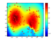
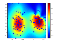
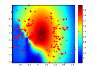
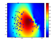
The first dataset is artificial-generated Ripleys synathetic [45]. The Ripleys synathetic comprise 250 training instances and 1000 testing instances. We visualize the distribution of fuzzy membership value for training instances under linear and nonlinear case in Fig. 3, respectively. As shown in Fig. 3, compared to those instances locating near the class center, the fuzzy membership values of the instances which are far from their class center are always smaller.
Refer to caption
(a) “+1” instances
Refer to caption
(b) “-1” instances
Refer to caption
(c) “+1” instances
Refer to caption
(d) “-1” instances
Figure 3: Fuzzy membership distribution of training instances on Ripley dataset. (a) and (b) for linear case, (c) and (d) for nonlinear case.
Refer to caption
Refer to caption
(a) SVM
Refer to caption
Refer to caption
(b) FSVM
Refer to caption
Refer to caption
(c) TSVM
Refer to caption
Refer to caption
(d) FR-TSVM
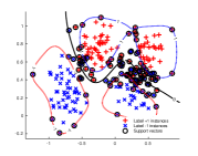
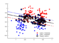
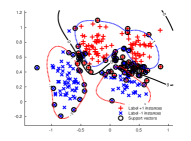
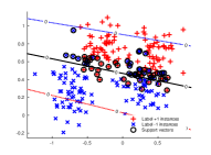
Figure 4: Results of linear and nonlinear SVM, FSVM, TSVM and FR-TSVM on the first artificial dataset (Ripleys synathetic). The first and second row show the results used linear kernel and Gaussian kernel, respectively. The blank straight line or curve represent the best decision hyperplane with corresponding method.

Table 4 reports testing accuracies and learning CPU time of all methods with linear and Gaussian kernel. We can see that linear SVM and nonlinear FR-TSVM achieve the highest prediction accuracy under linear and nonlinear case, respectively. The reason for the outperformance of linear SVM is more likely from the dataset itself than from the classifier because there may be no noise existing on the Ripleys synathetic dataset. The noiseless fact of this testing dataset suppresses the outstanding ability of FR-TSVM in the experiment. The ability of FR-TSVM is confirmed if we examine the accuracy in the nonlinear classification. In terms of execution time, FR-TSVM shows its excellence in computational efficiency for both linear and nonlinear learning, especially linear case. The excellence manifests the remarkable potential of employing FR-TSVM for fast classification.

Table 1: Classification performance comparison on artificial Ripleys dataset.
Methods Description   SVM  FSVM  TSVM FR-TSVM
Linear Acc(%percent\%)\uparrow 89.70 88.80 89.20 89.10
Time(s)\downarrow  1.46  2.00  0.28  0.21
Nonlinear Acc(%percent\%)\uparrow 90.40 91.10 90.50 91.30
Time(s)\downarrow  1.56  1.79  0.60  0.24

Fig. 4 shows linear and nonlinear decision hyperplanes produced by comparative methods with equivalent settings. In these panels, while standard SVM and FSVM produce only a single hyperplane (Fig. 4a and 4b), TSVM and FR-TSVM produce a pair of proximal hyperplanes (Fig. 4c and 4d) for class separation. Instead of single decision hyperplane in standard SVM and FSVM, a pair of nonparallel decision hyperplanes are used in TSVM and FR-TSVM. Comparing FR-TSVM with TSVM, the final decision hyperplane of FR-TSVM is more exact than one of TSVM. The fact reveals that FR-TSVM is more capable of producing an unbiased prediction than TSVM.

The second dataset is also a 2-dimensional artificial-generated dataset. In this dataset, the positive class of instances are generated by a uniform distribution satisfying x1[π/2,2π]subscript𝑥1𝜋22𝜋x_{1}\in[-\pi/2,2\pi], and sin(x1)0.25x2sin(x1)+0.25subscript𝑥10.25subscript𝑥2subscript𝑥10.25\sin(x_{1})-0.25\leq x_{2}\leq\sin(x_{1})+0.25, while the negative class of instances consist of uniform points satisfying x1[π/2,2π]subscript𝑥1𝜋22𝜋x_{1}\in[-\pi/2,2\pi], and 0.6sin(x1/1.05+0.5)1.3x20.6sin(x1/1.05+0.5)+0.80.6subscript𝑥11.050.51.3subscript𝑥20.6subscript𝑥11.050.50.80.6\sin(x_{1}/1.05+0.5)-1.3\leq x_{2}\leq 0.6\sin(x_{1}/1.05+0.5)+0.8, where x=[x1,x2]𝑥subscript𝑥1subscript𝑥2\vec{x}=[x_{1},x_{2}]. In our experiments, we generate 3000 instances according to the above rules. 600 instances are randomly chosen for training, and the remaining 2400 for testing.
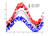
Refer to caption
Refer to caption
(a) SVM
Refer to caption
Refer to caption
(b) FSVM
Refer to caption
Refer to caption
(c) TSVM
Refer to caption
Refer to caption
(d) FR-TSVM
Figure 5: Results of nonlinear SVM, FSVM, TSVM and FR-TSVM on the second artificial dataset. Comparison of decision hyperplane with/without noises.
Table 2: Classification performance comparison on the second artificial dataset.
Methods Description   SVM  FSVM  TSVM FR-TSVM
nonoise Acc(%percent\%)\uparrow 99.92 99.88 99.92 100.0
Time(s)\downarrow 16.77 17.11  5.03  0.30
noise Acc(%percent\%)\uparrow 99.37 99.63 97.00 99.33
Time(s)\downarrow 16.43 16.74  4.93  0.72

In Fig. 5, the first row shows the results of the nonlinear SVM, FSVM, TSVM and the proposed FR-TSVM on this dataset. We can see that the separating hyperplanes of these classifiers obtain similar results. To further validate the robust performance of the FR-TSVM, we add a noise ε𝒩(0,0.2)𝜀𝒩00.2\varepsilon\in\mathcal{N}(0,0.2) for each training instance of this dataset, where 𝒩(0,0.2)𝒩00.2\mathcal{N}(0,0.2) is a normal distribution with mean 0 and variance 0.2. In Fig. 5, the second row shows the result of the nonlinear SVM, FSVM, TSVM and the proposed FR-TSVM on this dataset with noise. It can be seen that the proposed FR-TSVM can still effectively determine the separating hyperplane compared with the other three methods, especially TSVM. This indicates that the FR-TSVM can effectively alleviate the effect of noise points.

Table 2 reports prediction results including classification accuracy and training time with/without noises. We can see that all the methods obtain similarity test accuracies without noises, while our FR-TSVM achieves the highest test accuracy. Under noise case, FR-TSVM and FSVM obtain better classification accuracies than TSVM and SVM, respectively. This indicates that fuzzy membership takes an important role in training model with noisy instances. It is noteworthy that TSVM’s test accuracy is reduced by almost 3% (from 99.88% to 97.00%), whereas FR-TSVM has only a slight slowdown (less than 1%). It suggests that FR-TSVM is more robust than TSVM when training instances consist of noisy data. As for the training time, FR-TSVM and TSVM are more efficient than SVM and FSVM, while FR-TSVM is the fastest among all methods.

4.2 Experiments on benchmark datasets

To further examine the performance of FR-TSVM, 13 common datasets are gathered from the public UCI machine learning datasets [46]. To adjust values measured on different scales to a notionally common scale in the input space, all input features are normalized and scaled-down within [0,1]01[0,1]. The examination mainly focuses on binary classification. Two adversary classes are formed in every dataset. For the multi-classification datasets, we convert them into binary classification datasets by taking the majority class as the first class and gathering all the remainders together as the adversary class. Table 3 lists the statistics of datasets.

Table 4 and 5 report the learning results of these algorithms with linear and Gaussian kernels. To show the optimization cost, a particular quadratic programming time is recorded. To assess the performance, 10-folds cross-validation, as that in Section 4, is taken. It means every classifier is repeatedly validated in the datasets with a ratio of 90%/10% for respective training/testing phase. Ten characteristics values are collected and averaged for the assessment. In the experiments, a standard deviation of the ten classification accuracies is provided in addition to the average to reflect the classification robustness.

Table 3: Detailed characteristics of the benchmark datasets. l𝑙l, l+subscript𝑙l_{+} and lsubscript𝑙l_{-} are the number of all instances, positive instances and negative instances, respectively. n𝑛n is the dimension of feature.
Dataset Data statistics
#l#𝑙\#l #l+#subscript𝑙\#l_{+} #l#subscript𝑙\#l_{-} #n#𝑛\#n
Breast 106 22 84 9
Ionosphere 351 126 225 34
Iris 150 100 50 4
Australian 690 307 383 14
WDBC 569 357 212 30
Wine 178 119 59 13
Hepatitis 155 123 32 19
WPBC 198 46 148 33
Bupa 345 200 145 6
Sonar 208 111 97 60
Glass 214 138 76 10
Heart 270 120 150 13
Pima 768 268 500 8
Table 4: Comparison results (mean±plus-or-minus\pmstd) of linear SVM, FSVM, TSVM and FR-TSVM on benchmark datasets. The best result of each row is marked in bold.
Dataset SVM FSVM TSVM FR-TSVM
Breast 96.33±plus-or-minus\pm4.77 97.17±plus-or-minus\pm4.58 97.17±plus-or-minus\pm4.58 97.17±plus-or-minus\pm4.58
Ionosphere 83.53±plus-or-minus\pm6.48 85.75±plus-or-minus\pm4.06 82.33±plus-or-minus\pm5.18 87.19±plus-or-minus\pm4.22
Iris 100.0±plus-or-minus\pm0.00 100.0±plus-or-minus\pm0.00 100.0±plus-or-minus\pm0.00 100.0±plus-or-minus\pm0.00
Australian 84.92±plus-or-minus\pm4.53 85.50±plus-or-minus\pm4.59 85.07±plus-or-minus\pm4.77 85.93±plus-or-minus\pm4.39
WDBC 95.34±plus-or-minus\pm5.17 95.87±plus-or-minus\pm3.21 93.84±plus-or-minus\pm5.86 96.39±plus-or-minus\pm3.52
Wine 98.89±plus-or-minus\pm2.34 98.89±plus-or-minus\pm2.34 98.33±plus-or-minus\pm2.68 98.89±plus-or-minus\pm2.34
Hepatitis 79.26±plus-or-minus\pm8.76 84.94±plus-or-minus\pm7.29 75.58±plus-or-minus\pm12.50 85.77±plus-or-minus\pm7.21
WPBC 79.93±plus-or-minus\pm9.49 74.24±plus-or-minus\pm10.35 76.88±plus-or-minus\pm7.01 77.96±plus-or-minus\pm10.03
Bupa 66.36±plus-or-minus\pm6.04 67.51±plus-or-minus\pm7.36 61.72±plus-or-minus\pm5.96 64.38±plus-or-minus\pm6.24
Sonar 74.08±plus-or-minus\pm8.96 77.46±plus-or-minus\pm7.14 72.15±plus-or-minus\pm7.48 78.34±plus-or-minus\pm8.29
Glass 70.41±plus-or-minus\pm10.01 74.18±plus-or-minus\pm11.01 67.64±plus-or-minus\pm11.02 81.17±plus-or-minus\pm13.56
Heart 82.22±plus-or-minus\pm5.18 82.59±plus-or-minus\pm3.51 84.07±plus-or-minus\pm4.95 84.07±plus-or-minus\pm6.06
Pima 77.21±plus-or-minus\pm3.75 75.65±plus-or-minus\pm4.22 76.95±plus-or-minus\pm3.37 75.13±plus-or-minus\pm3.78
Table 5: Comparison results (mean±plus-or-minus\pmstd) of nonlinear SVM, FSVM, TSVM and FR-TSVM on benchmark datasets. The best result of each row is marked in bold.
Dataset SVM FSVM TSVM FR-TSVM
Breast 97.26±plus-or-minus\pm4.43 97.17±plus-or-minus\pm4.58 96.33±plus-or-minus\pm4.77 98.09±plus-or-minus\pm4.03
Ionosphere 94.84±plus-or-minus\pm4.01 94.59±plus-or-minus\pm4.31 92.61±plus-or-minus\pm6.12 95.41±plus-or-minus\pm4.93
Iris 100.0±plus-or-minus\pm0.00 100.0±plus-or-minus\pm0.00 100.0±plus-or-minus\pm0.00 100.0±plus-or-minus\pm0.00
Australian 85.50±plus-or-minus\pm4.53 85.50±plus-or-minus\pm4.59 85.50±plus-or-minus\pm4.59 86.81±plus-or-minus\pm4.84
WDBC 94.84±plus-or-minus\pm4.23 95.34±plus-or-minus\pm3.80 95.34±plus-or-minus\pm3.80 96.39±plus-or-minus\pm3.52
Wine 99.44±plus-or-minus\pm1.76 98.89±plus-or-minus\pm2.34 100.0±plus-or-minus\pm0.00 100.0±plus-or-minus\pm0.00
Hepatitis 80.51±plus-or-minus\pm8.32 84.28±plus-or-minus\pm7.42 82.00±plus-or-minus\pm6.84 84.48±plus-or-minus\pm6.86
WPBC 81.51±plus-or-minus\pm7.13 77.88±plus-or-minus\pm9.43 75.30±plus-or-minus\pm7.93 82.51±plus-or-minus\pm8.05
Bupa 70.68±plus-or-minus\pm8.28 72.71±plus-or-minus\pm7.93 71.86±plus-or-minus\pm5.71 71.84±plus-or-minus\pm5.67
Sonar 89.42±plus-or-minus\pm5.41 88.92±plus-or-minus\pm6.95 89.42±plus-or-minus\pm5.41 89.44±plus-or-minus\pm5.31
Glass 97.68±plus-or-minus\pm3.95 96.77±plus-or-minus\pm4.38 94.87±plus-or-minus\pm5.08 97.21±plus-or-minus\pm3.93
Heart 84.07±plus-or-minus\pm5.25 82.59±plus-or-minus\pm4.29 80.74±plus-or-minus\pm7.16 84.81±plus-or-minus\pm4.08
Pima 75.65±plus-or-minus\pm3.80 75.26±plus-or-minus\pm2.91 77.34±plus-or-minus\pm5.16 76.17±plus-or-minus\pm2.68

Comparing to baselines including SVM, FSVM and TSVM, the FR-TSVM produces more competitive and robust performances (e.g, high mean and low deviation of accuracies) on most datasets in Table 4 and 5. This suggests it is important to improve the classification performance introducing the fuzzy membership. Moreover, the tables show a higher improvement using nonlinear kernel than that of a linear kernel. This is due to the intrinsic difference between the kernels. As we know, a nonlinear Gaussian kernel commonly pertains a superior classification ability due to its flexibility. It meets the general concept of the classification. In addition, FR-TSVM obtains slightly lower performance than other methods on a few datasets (e.g, Bupa and Pima). A possible reason is that these datasets may not have outliers. Fig. 6 shows the time cost of training on 13 UCI datasets. It is seen that the training time of TSVM and FR-TSVM are shorter than those of SVM and FSVM. This result is not surprising because TSVM and FR-TSVM are solved by two small QPPs rather than one large QPP in SVM and FSVM. Compared to the training time of TSVM, our FR-TSVM are faster. In short, the results in Table 4 and 5 indicate, FR-TSVM effectively improves the classification accuracy and efficiently reduces training time compared to the traditional methods. The excellence strongly reflects that the classifier is potential for future applications.

Refer to caption
Refer to caption
(a)
Refer to caption
Refer to caption
(b)
Refer to caption
Refer to caption
(c)
Refer to caption
Refer to caption
(d)
Refer to caption
Refer to caption
(e)
Refer to caption
Refer to caption
(f)
Refer to caption
Refer to caption
(g)
Refer to caption
Refer to caption
(h)
Refer to caption
Refer to caption
(i)
Refer to caption
Refer to caption
(j)
Refer to caption
Refer to caption
(k)
Refer to caption
Refer to caption
(l)
Refer to caption
Refer to caption
(m)
Figure 6: Comparison of training time on thirteen benchmark datasets including (a)Breast (b)Ionosphere (c)Iris (d)Australian (e)WDBC (f)Wine (g)Hepatitis (h)WPBC (i)Bupa (j)Sonar (k)Glass (l)Heart and (m)Pima.

4.3 Parameter analysis

Refer to caption
(a) μ=0.1𝜇0.1\mu=0.1, g=1𝑔1g=1
Refer to caption
(b) μ=0.1𝜇0.1\mu=0.1, c1=32subscript𝑐132c_{1}=32
Refer to caption
(c) μ=0.1𝜇0.1\mu=0.1, c3=0.5subscript𝑐30.5c_{3}=0.5
Refer to caption
(d) c1=32subscript𝑐132c_{1}=32, c3=0.5subscript𝑐30.5c_{3}=0.5
Figure 7: Accuracy varying adjustable parameters of nonlinear FR-TSVM on Ripleys dataset.

FR-TSVM’s performance may be affected by hyperparameters. The hyperparameters corresponding to the investigation are those c1=c2subscript𝑐1subscript𝑐2c_{1}=c_{2}, c3=c4subscript𝑐3subscript𝑐4c_{3}=c_{4}, u𝑢u, and g𝑔g in Gaussian kernel for nonlinear case. Here, we take Ripleys synathetic dataset for an example.

Fig. 7 further shows the test accuracy with varying the adjustable parameters on artificial dataset Ripleys synathetic. Despite artificial dataset, two points are thus eventually asserted from the investigation. First, each adjustable parameter affects significantly the FR-TSVM’s performance, especially Gaussian kernel parameter g𝑔g. Second, the inconsistent trends of the accuracy with respect to the parameters reveal that the issue of parameter selection is still a challenge for us. We thus leave the issue as a future study.

5 Conclusion

In this paper, we propose a FR-TSVM algorithm for binary classification based on FSVM, TSVM and coordinate descent methods. First, similar to FSVM classifier, the embedded fuzzy concept enhances noise-resistance capability and generalization ability. However, the fuzzy membership construction is different from that of the FSVM. Our method can effectively assign the fuzzy membership value to different instances by distinguishing the support vectors and the outliers. Second, as TSVM, the FR-TSVM finds a pair of nonparallel hyperplanes through two smaller sized QPPs rather than one large-sized QPP in the SVM or FSVM. As we all know, the dual problems of the TSVM may be ill-conditioned, but the proposed model’s dual form has been brought to a pair of convex quadratic programming problems and confirmed it is capable of solution uniqueness and singularity avoidance. Third, a novel coordinate descent method with shrinking is developed to solve the dual problems. Compared to TSVM, our FR-TSVM is not only faster but also needs less memory storage. This indicates that our FR-TSVM is very suitable for large-scale data. Experiments with simulated and realistic datasets reveal that an exceedingly high classification accuracy with less computation time is achieved using both linear or nonlinear FR-TSVM. However, there are 6 parameters (i.e., c1,c2,c3,c4,μ,gsubscript𝑐1subscript𝑐2subscript𝑐3subscript𝑐4𝜇𝑔c_{1},c_{2},c_{3},c_{4},\mu,g) in our FR-TSVM, so the parameters selection is a practical problem and should be addressed in the future. Also, it is an interesting direction to extend FR-TSVM to more recognition problems such as multi-class or multi-label problem.

References

References

  • [1] V. Vapnik, Statistical learning theory, Wiley New York, 1998.
  • [2] A. Widodo, B.-S. Yang, Support vector machine in machine condition monitoring and fault diagnosis, Mechanical Systems and Signal Processing 21 (6) (2007) 2560–2574.
  • [3] B. Heisele, P. Ho, T. Poggio, Face recognition with support vector machines: Global versus component-based approach, in: Proc. IEEE Int’l Conf. Computer Vision, IEEE, 2001, pp. 688–694.
  • [4] T. Joachims, Text categorization with support vector machines: Learning with many relevant features, in: European Conference on Machine Learning, Springer, 1998, pp. 137–142.
  • [5] I. El-Naqa, Y. Yang, M. N. Wernick, N. P. Galatsanos, R. M. Nishikawa, A support vector machine approach for detection of microcalcifications, IEEE Trans. on Medical Imaging 21 (12) (2002) 1552–1563.
  • [6] T. B. Trafalis, H. Ince, Support vector machine for regression and applications to financial forecasting., in: Proc. Int’l Joint Conf. on Neural Networks, 2000, pp. 348–353.
  • [7] O. L. Mangasarian, E. W. Wild, Multisurface proximal support vector machine classification via generalized eigenvalues, IEEE Trans. on Pattern Analysis and Machine Intelligence 28 (1) (2006) 69–74.
  • [8] R. Jayadeva, Khemchandani, S. Chandra, Twin support vector machines for pattern classification, IEEE Trans. on Pattern Analysis and Machine Intelligence 29 (5) (2007) 905–910.
  • [9] Y.-H. Shao, C.-H. Zhang, X.-B. Wang, N.-Y. Deng, Improvements on twin support vector machines, IEEE Trans. on Neural Networks 22 (6) (2011) 962–968.
  • [10] Z. Qi, Y. Tian, Y. Shi, Structural twin support vector machine for classification, Knowledge-Based Systems 43 (2013) 74–81.
  • [11] Z.-Q. Qi, Y.-J. Tian, Y. Shi, Robust twin support vector machine for pattern classification, Pattern Recognition 46 (1) (2013) 305–316.
  • [12] W.-J. Chen, Y.-H. Shao, N. Hong, Laplacian smooth twin support vector machine for semi-supervised classification, Int’l Journal of Machine Learning and Cybernetics 5 (3) (2014) 459–468.
  • [13] M. A. Kumar, M. Gopal, Least squares twin support vector machines for pattern classification, Expert Systems with Applications 36 (4) (2009) 7535–7543.
  • [14] J. A. Nasiri, N. M. Charkari, S. Jalili, Least squares twin multi-class classification support vector machine, Pattern Recognition 48 (3) (2015) 984–992.
  • [15] X. Peng, TPMSVM: a novel twin parametric-margin support vector machine for pattern recognition, Pattern Recognition 44 (10) (2011) 2678–2692.
  • [16] X. Peng, L. Kong, D. Chen, Improvements on twin parametric-margin support vector machine, Neurocomputing 151 (2015) 857–863.
  • [17] W.-J. Chen, Y.-H. Shao, C.-N. Li, N.-Y. Deng, MLTSVM: A novel twin support vector machine to multi-label learning, Pattern Recognition 52 (2016) 61–74.
  • [18] R. Rastogi, S. Sharma, S. Chandra, Robust parametric twin support vector machine for pattern classification, Neural Processing Letters (2017) 1–31.
  • [19] Y. Xu, Z. Yang, X. Pan, A novel twin support-vector machine with pinball loss, IEEE transactions on neural networks and learning systems 28 (2) (2017) 359–370.
  • [20] X. Peng, TSVR: an efficient twin support vector machine for regression, Neural Networks 23 (3) (2010) 365–372.
  • [21] X. Peng, D. Xu, J. Shen, A twin projection support vector machine for data regression, Neurocomputing 138 (2014) 131–141.
  • [22] Y.-F. Ye, L. Bai, X.-Y. Hua, Y.-H. Shao, Z. Wang, N.-Y. Deng, Weighted lagrange ε𝜀\varepsilon-twin support vector regression, Neurocomputing 197 (2016) 53–68.
  • [23] R. Khemchandani, K. Goyal, S. Chandra, Twsvr: regression via twin support vector machine, Neural Networks 74 (2016) 14–21.
  • [24] R. Rastogi, P. Anand, S. Chandra, A ν𝜈\nu-twin support vector machine based regression with automatic accuracy control, Applied Intelligence 46 (3) (2017) 670–683.
  • [25] C.-F. Lin, S.-D. Wang, Fuzzy support vector machines, IEEE Trans. on Neural Networks 13 (2) (2002) 464–471.
  • [26] C.-F. Lin, et al., Training algorithms for fuzzy support vector machines with noisy data, Pattern recognition letters 25 (14) (2004) 1647–1656.
  • [27] Y. Wu, Y. Liu, Robust truncated hinge loss support vector machines, Journal of the American Statistical Association.
  • [28] T. Inoue, S. Abe, Fuzzy support vector machines for pattern classification, in: Proc. Int’l Joint Conf. on Neural Networks, IEEE, 2001, pp. 1449–1454.
  • [29] C.-Y. Yang, J.-J. Chou, F.-L. Lian, Robust classifier learning with fuzzy class labels for large-margin support vector machines, Neurocomputing 99 (2013) 1–14.
  • [30] W. M. Tang, Fuzzy svm with a new fuzzy membership function to solve the two-class problems, Neural Processing Letters 34 (3) (2011) 209–219.
  • [31] Y. Xu, L. Wang, P. Zhong, A rough margin-based ν𝜈\nu-twin support vector machine, Neural Computing and Applications 21 (6) (2012) 1307–1317.
  • [32] R. Khemchandani, C. S. Jayadeva, Fuzzy twin support vector machines for pattern classification, Mathematical Programming and Game Theory for Decision Making. (2008) 131–42.
  • [33] B. Richhariya, M. Tanveer, A robust fuzzy least squares twin support vector machine for class imbalance learning, Applied Soft Computing 71 (2018) 418–432.
  • [34] T. Kudo, Y. Matsumoto, Chunking with support vector machines, in: Proc. North American Chapter of the Association for Computational Linguistics on Language technologies, Association for Computational Linguistics, 2001, pp. 1–8.
  • [35] J.-X. Dong, A. Krzyżak, C. Y. Suen, Fast svm training algorithm with decomposition on very large data sets, IEEE Trans. on Pattern Analysis and Machine Intelligence 27 (4) (2005) 603–618.
  • [36] J. C. Platt, Fast training of support vector machines using sequential minimal optimization, in: Advances in kernel methods—Support Vector Learning, MIT Press, 1999, pp. 185–208.
  • [37] C.-C. Chang, C.-J. Lin, LIBSVM: A library for support vector machines, ACM Trans. on Intelligent Systems and Technology 2 (3) (2011) 27, software available at http://www.csie.ntu.edu.tw/~cjlin/libsvm.
  • [38] K.-W. Chang, C.-J. Hsieh, C.-J. Lin, Coordinate descent method for large-scale l2-loss linear support vector machines, The Journal of Machine Learning Research 9 (2008) 1369–1398.
  • [39] C.-J. Hsieh, K.-W. Chang, C.-J. Lin, S. S. Keerthi, S. Sundararajan, A dual coordinate descent method for large-scale linear svm, in: Proc. of the 25th int’l conf. on Machine learning, ACM, 2008, pp. 408–415.
  • [40] B.-B. Gao, J.-J. Wang, Y. Wang, C.-Y. Yang, Coordinate descent fuzzy twin support vector machine for classification, in: Proceedings of the IEEE Conference on Machine Learning and Applications (ICMLA), 2015, pp. 7–12.
  • [41] A. J. Smola, B. Schölkopf, Learning with kernels, Citeseer, 1998.
  • [42] Y.-H. Shao, N.-Y. Deng, A coordinate descent margin based-twin support vector machine for classification, Neural Networks 25 (2012) 114–121.
  • [43] M. O’Searcoid, Metric spaces, Springer Science & Business Media, 2006.
  • [44] A. Messac, Optimization in Practice with MATLAB®: For Engineering Students and Professionals, Cambridge University Press, 2015.
  • [45] B. D. Ripley, Pattern recognition and neural networks, Cambridge university press, 1996.
  • [46] C. Blake, C. J. Merz, UCI repository of machine learning databases, available at http://~archive.ics.uci.edu/ml/about.html (1998).