Quantum Algorithm for Simulating the Wave Equation
Abstract
We present a quantum algorithm for simulating the wave equation under Dirichlet and Neumann boundary conditions. The algorithm uses Hamiltonian simulation and quantum linear system algorithms as subroutines. It relies on factorizations of discretized Laplacian operators to allow for improved scaling in truncation errors and improved scaling for state preparation relative to general purpose linear differential equation algorithms. We also consider using Hamiltonian simulation for Klein-Gordon equations and Maxwell’s equations.
1 Introduction
Here we present a quantum algorithm for simulating the wave equation, subject to nontrivial boundary conditions. In particular, the algorithm can simulate the scattering of a wave packet off of scatterers of arbitrary shape, with either Dirichlet or Neumann boundary conditions. The output of the simulation is in the form of a quantum state proportional to the solution to the wave equation. By measuring this state one obtains a sample from a distribution proportional to the square of the amplitude, which in this case can be interpreted as the intensity of the wave.
Compared to classical algorithms, our method uses a number of qubits that scales only logarithmically with the number of lattice sites, whereas classical methods require a number of bits scaling linearly with the number of lattice sites. Additionally, for simulating the wave equation in a region of diameter in -dimensions, discretized onto a lattice of spacing , our quantum algorithm has a state-preparation step with time complexity and a Hamiltonian simulation step with time complexity , where is the evolution time for the wave equation. In contrast, all classical algorithms outputting a full description of the field, whether based on finite difference methods or finite element methods, must have time complexity scaling at least linearly with the number of lattice sites, i.e. as .
Several prior works give quantum algorithms for related problems. Berry gave an algorithm for first order linear differential equations that encodes a linear multistep method into a linear system which is then solved using a quantum linear system algorithm [1]. This algorithm was recently improved upon in [2] which gives an algorithm that scales better than the algorithm of [1] with respect to several system parameters. Through standard transformations, the wave equation in a region of diameter can be discretized onto a lattice of spacing and transformed into a system of linear first order differential equations, which could then in general be solved by the quantum algorithms of [1, 2] with complexity of order . (See §11.) The complexity the quantum algorithm that we present here scales linearly with . This quadratic improvement is achieved in exchange for being specialized for solving wave equations rather than general linear differential equations. At even greater generality, Leyton and Osborne proposed an algorithm for a class of nonlinear initial value problems [3]. This greater generality comes at a further cost in performance in that the complexity of the quantum algorithm scales exponentially with the evolution time. Related work on quantum algorithms for solving the Poisson equation can be found in [4].
The improved scaling of our algorithm relies on higher order approximations of the Laplacian operator and their factorizations using hypergraph incidence matrices. We describe how to find these operators and their hypergraph incidence matrices, and we provide numerical values for up to tenth order. (Throughout this manuscript we use the term order Laplacian to mean a discretization of the Laplacian which, when used on a lattice of spacing , has leading error term of order .) To our knowledge, these hypergraph incidence matrix factorizations do not appear elsewhere in the literature. These higher order Laplacians also allow us to improve how errors scale with respect to lattice spacing at the cost of simulating more complex (less sparse) Hamiltonians. In particular, using a -sparse Hamiltonian to simulate the wave equation for a volume of diameter in dimensions produces error on the order of , so scales as (where is the error in the state output by the algorithm). Expressing the time complexity of our algorithm in terms of and , we find that the state preparation has time complexity and the Hamiltonian simulation has time complexity . Generally is an integer multiple of , so these complexities scale polynomially in even though appears in an exponent.
In [5], Jacobs, Clader, and Sprouse proposed a quantum algorithm for calculating electromagnetic scattering cross-sections that is based on solving boundary value problems in the special case of monochromatic waves. This monochromaticity assumption allows separation of variables thereby reducing the calculation to a time-independent problem.
Rather than finite-difference methods, as discussed here, it is also possible to obtain approximate solutions to the full time-dependent wave equation through finite element methods such as the Galerkin method. In [6] Montanaro and Pallister analyze, in a general context, the degree to which quantum linear algebra methods such as [7, 8] allow speedup for finite element methods. Detailed analysis of how this can be applied to the wave equation specifically, particularly with the aid of preconditioners, is a complex subject which we defer to future work.
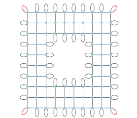
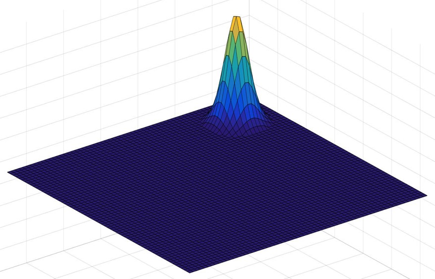
Following [5] we consider as our primary application the simulation of scattering in complicated geometries 111Note that, the presence of a scatterer breaks translational invariance and consequently the Laplacian cannot simply be diagonalized by a Fourier transform., as illustrated in figure 1. In this case, the initial condition at time zero is a localized wave packet and its time derivative, and the final output of the simulation algorithm is an estimate of the intensity of the wave at a later time within some region of space occuppied by the detector. After discretizing space, the scatterer can be modeled as a hole in the lattice where some points have been removed. Dirichlet or Neumann boundary conditions can be imposed on the boundary of this hole, as discussed in §3. In §4 we describe how to accommodate various initial conditions in our approach. In §5 we provide numerical evidence that our approach accurately simulates the wave equation with appropriate behavior at boundaries. In §6 and §7 we describe higher order approximations of the Laplacian operator which allow for more precise approximations. In §8 we provide numerical confirmation that higher order Laplacians improve how errors scale. In §10 we discuss the post-processing step which follows Hamiltonian simulation. In §11 we compare our approach to other quantum algorithms for the wave equation. In §12 and §13 we address the use of Hamiltonian simulation for simulating the Klein-Gordon equation and Maxwell’s equations, respectively.

2 Algorithm
In any number of dimensions, the wave equation is
| (1) |
To avoid cumbersome notation, in the rest of this paper we will take the wave propagation speed to be . For a given initial condition specifying and at , our goal is to obtain a quantum state encoding the solution determined by (1) at some later time .
To achieve this, we will first discretize space. We can then think of as a matrix acting on a vector whose entries encode the value of the field at each point in discrete space (with appropriate boundary conditions). Discrete approximations of the Laplacian operator have been thoroughly studied in both spectral graph theory and quantum chemistry, and we draw upon this previous work. In the simplest case, we can discretize a finite region of onto a cubic grid of lattice spacing . The resulting points can be thought of as a graph , with edges between nearest neighbors. The corresponding graph Laplacian is the square matrix whose rows and columns index the vertices of this graph, and whose off-diagonal matrix elements are minus one for connected vertices and zero otherwise. Each diagonal matrix element is equal to the degree of the corresponding vertex, i.e. the number of other vertices it is connected to. The operator approximates in the limit . For example, in one dimension:
| (2) |
which becomes the second derivative of in the limit . At finite the truncation error is .
After discretization, we are faced with the task of simulating
| (3) |
To this end, consider a Hamiltonian of the following block form, which by construction is Hermitian independent of the specific choice of matrix .
| (4) |
Schrödinger’s equation then takes the form
| (5) |
which implies
| (6) | ||||
| (7) |
So, if then a subspace of the full Hilbert space evolves according to a discretized wave equation.
For any graph, weighted or unweighted, and with or without self-loops, is achieved by taking to be the corresponding signed incidence matrix, defined as follows. For a given graph with vertices and edges, is an matrix with rows indexed by vertices and columns indexed by edges. One starts by arbitrarily assigning orientations to the edges of the graph. This arbitrary choice affects but does not affect , which always equals the Laplacian of the undirected graph. The general definition of the incidence matrix for a graph where edge has weight is
| (8) |
In the special case that the graph is unweighted, for every edge.
From the above, one sees that the Hilbert space associated with the graph is
| (9) |
where is the vertex space (where is supported) and is the edge space (where is supported). The dynamics on the vertex space obeys the discretized wave equation. The amplitudes associated with the edges are extra variables that necessarily arise when converting second order differential equations into first order differential equations.
Simulating the time evolution according to (5) can be achieved using state of the art quantum algorithms for simulating the dynamics induced by general sparse Hamiltonians. One sees that the dimension of the Hilbert space is equal to the number of vertices of the graph plus the number of edges: + . In particular, for a cubic region of side-length in -dimensions, discretized into a cubic grid of lattice spacing , one has and . Thus, the number of qubits needed is . The largest matrix element of has magnitude , and the number of nonzero matrix elements in each row or column of is at most .
Using the method of [9] we can approximate the unitary time evolution to within using a quantum circuit of
| (10) |
gates, where , where is the largest matrix element of in absolute value, and . For the Hamiltonian of (4), , , and , and therefore the total complexity of simulating the time-evolution is
| (11) | |||||
where the notation indicates that we are suppressing logarithmic factors. The table below compares the asymptotic runtime and memory usage of our algorithm against standard classical numerical methods for solving differential equations.
| Classical | Quantum | |
|---|---|---|
| Time | ||
| Space |
The remaining considerations are the implementation of desired boundary conditions, the preparation of an initial state implementing the desired initial conditions, errors induced by discretizing the wave equation, and the relative probability to obtain samples from the vertex space versus the edge space at the end of the computation. In the following sections we address each of these issues in turn. These considerations motivate various improvements and extensions to the above algorithm, which we introduce along the way, in particular the use of higher order discretizations of .
3 Boundary Conditions
Here we will consider how to implement two commonly used boundary conditions: Dirichlet and Neumann. With Dirichlet boundary conditions at the boundary. With Neumann boundary conditions at the boundary, where is the unit vector normal to the boundary. For any shape of boundary and in any number of dimensions our prescription is as follows. To implement Neumann boundary conditions use the ordinary graph Laplacian of the graph obtained by starting with the cubic grid and removing the vertices interior to the scattering object. To implement Dirichlet boundary conditions one must add weighted self-loops to each of the vertices on the boundary with weights equal to the number of edges that are missing relative to interior vertices. (This ensures that the diagonal matrix elements of the resulting graph Laplacian are all equal.) See figure 2 for an illustration. For pedagogical reasons, we give two derivations of the Laplacians implementing these boundary conditions, using the one dimensional path graph as an example. One derivation is based on discretization of derivatives, and the other is by linear algebra on an already-discretized system.
Neumann Boundary Conditions by Discretization
Consider the line segment . Within this, the second derivative discretizes to
| (12) |
This yields at internal vertices the familiar form of a discrete Laplacian.
| (13) |
With Neumann boundary conditions, at the boundaries. Thus, at the leftmost vertex we have:
Similarly, vanishes at the rightmost vertex. For example, if we discretize the segment into five lattice sites we would have
| (15) |
is recognizable as the ordinary graph Laplacian for the path graph of five vertices:
.
This holds more generally; the ordinary graph Laplacian on discretized regions of any shape in any number of dimensions yields Neumann boundary conditions. Note that in the above example discretizing the unit interval with five vertices, one should take because each of the four edges in the graph corresponds to a distance of , but as we see from the above argument, the boundary conditions correspond to at and .
Neumann Boundary Conditions, Algebraic Derivation
We first consider the Laplacian for an infinite path graph with vertices labeled by , which is a tridiagonal matrix with 2 on the diagonal and -1 on the off-diagonals. It suffices to consider imposing the boundary conditions at the left end of the interval, which we assume corresponds to the vertex 0 in our discrete space. Then for Neumann boundary conditions the field is constant on all vertices , that is . Then consider how acts on the field in the neighborhood of 0. We represent this as
| (16) | ||||
| (17) | ||||
| (18) |
So we see that imposing Neumann boundary conditions allows us to ignore the vertices labeled by negative numbers. To give a finite example, if we restrict to the vertices (i.e. impose Neumann boundary conditions for vertices to the left of 0 and to the right of 3) then the Laplacian we produce is
| (19) |
which is exactly the graph Laplacian for the path graph on 4 vertices.
Dirichlet Boundary Conditions, Algebraic Derivation
We use similar arguments to show how to impose Dirichlet boundary conditions. Consider imposing to the left of . Then acts as
| (20) | ||||
| (21) | ||||
| (22) |
Since we are only concerned with how the Laplacian acts on vertices and not on we can ignore the fact that . Another way to motivate this is that by restricting the wave equation to act on vertices we do not provide a dynamical equation for , so it will remain 0.
To compare this with the Neumann case, if we restrict to the vertices then the Laplacian we produce is
| (23) |
which differs from the Neumann Laplacian in the upper-left and lower-right entries.
4 Initial Conditions
The first step in our quantum algorithm is to prepare a quantum state corresponding to desired initial conditions and at . Our method for preparing the initial state and its complexity varies depending on the specific type of initial conditions.
As a first example, consider a line-segment with Dirichlet boundary conditions, discretized into four lattice sites. In this case, by (4) and (8), we have
| (24) |
This can be viewed as a discretization of
| (25) |
where we use the forward difference to approximate and the backward difference to approximate . More generally, in an arbitrary number of dimensions, the Hamiltonian (4) can be seen as a discretization of
| (26) |
(We here view as describing a vector field, where the value associated with a given edge in the graph is the vector component along the direction that the edge points.) Consequently, for an arbitrary initial condition specified by and one must prepare a corresponding initial quantum state that is a solution to
| (27) |
In more than one dimension, the equation (27) does not uniquely determine since is unspecified. (In one dimension is determined up to an additive constant.) In the remainder of this section we consider how to compute a solution to (27) and how to prepare the initial state on a quantum computer in various cases of interest.
4.1 Static Initial State
The simplest case is to prepare a state with uniformly equal to zero. Then, one can use as an initial quantum state. The state preparation problem then reduces to preparing ; however, this is not necessarily efficient for arbitrary . Preparation of a completely arbitrary quantum state in an -dimensional Hilbert space has complexity of order , i.e. exponential in the number of qubits. Specifically, suppose one were given an oracle, which when queried with a bit string returned a corresponding amplitude written (to some number of bits of precision) into an output register. One wishes to prepare the corresponding quantum state . The worst-case complexity of this task is [10]. In many cases of interest, the complexity for preparing the initial state may be much lower. In particular, as was originally shown in [11], a state of the form
| (28) |
can be prepared in poly() time on a quantum computer provided that each of the conditional probabilities
| (29) |
can be efficiently computed. As discussed in [12], these conditional probabilities can be efficiently computed for all log-concave probability distributions.
4.2 Rigidly Translating Wave packet
In one spatial dimension, for any twice-differentiable wave packet shape ,
| (30) |
is a solution to the wave equation . (In this manuscript we will generally take .) From (25) one sees that the quantum state
| (31) |
represents this solution in the continuum limit. For a lattice with Neumann or Dirichlet boundary conditions, the vertex and edge Hilbert spaces have different dimensions, so the initial state is not merely where . This can be overcome by instead preparing where and . So if the quantum state (suitably discretized in each Hilbert space) can be prepared in polynomial time then so can the state (31). More generally, in an arbitrary number of dimensions, one can obtain an analogous initial state proportional to
| (32) |
with . This initially represents a wave packet traveling with velocity , but unlike in the one dimensional case, the wave packet will evetually suffer dispersion rather than simply translating rigidly.
4.3 General Case
In the general case we may imagine that we are given efficient quantum circuits preparing the states and . The discrete analogue of (27) is, via our incidence-matrix discretization:
| (33) | |||||
| (34) |
In two and higher dimensions, the solution to is non-unique in general since the number of edges in the graph exceeds the number of vertices. Thus, the number of columns of exceeds the number of rows by a factor of order , the number of spatial dimensions. One valid solution is to use as our quantum initial state
| (35) |
where denotes the Moore-Penrose pseudoinverse of the matrix . A Moore-Penrose pseudoinverse has the property that the image of is the orthogonal complement of the kernel of . Recall that is a map from . For the case of the standard 2nd order Laplacian, the corresponding is the signed incidence matrix of a graph. In this case can be interpreted in the continuum limit as a divergence. The Helmholtz decomposition theorem says that any twice-differentiable vector field can be decomposed into a curl-free component and a divergence-free component, the latter of which corresponds to the kernel of in the continuum limit. Thus, corresponds in the continuum limit to the solution to the following system of equations.
| (36) | |||||
| (37) |
To construct the state (35) we can use the quantum linear systems algorithm of [8]. Specifically, we wish to prepare the state proportional to the solution to where
| (40) | |||||
| (43) |
This can be done using the quantum linear systems algorithm of [8], whose time complexity is , where is the condition number of , which in this case is equal to the condition number of the incidence matrix .
Using the state (35) restricts the classes of solutions which our algorithm simulates. This is because does not have support in the kernel of . This is significant for Neumann boundary conditions because the kernel of (and of the Laplacian) is the all-ones vector, whereas for Dirichlet boundary conditions the kernel is trivial. This means that, even if had support in the space spanned by the all-ones vector, the algorithm will simulate the system with the modified initial condition where does not have support in this space. This restriction may seem artificial, but it is a natural consequence of the unitarity of Hamiltonian dynamics. If the uniform support of were not projected out, then our algorithm would be able to simulate the solution (with no dependence on ) for which is constant. This would result in the norm of the quantum state changing in time, in contradiction to unitarity.
In more detail, an algorithm from [8] can perform the transformation using a number of gates that scales as where is the sparsity of , is the condition number of and is the dimension of the Hilbert space. The condition number of is the square root of the condition number of the graph Laplacian . has norm and smallest eigenvalue , independent of , where the volume under consideration is which discretized onto a grid of spacing . Thus . The sparsity of is for any fixed order of discretization, and the Hilbert space dimension is . Putting this together yields an overall complexity of for state preparation in this case (neglecting log factors).
5 Numerical Examples
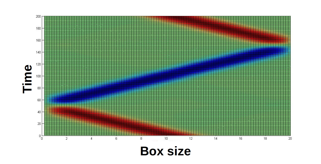
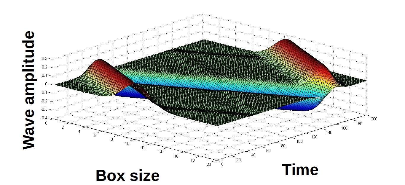
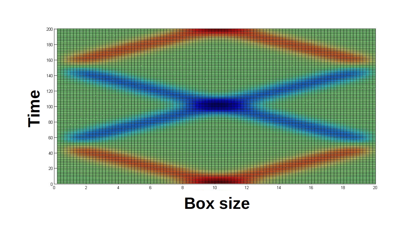
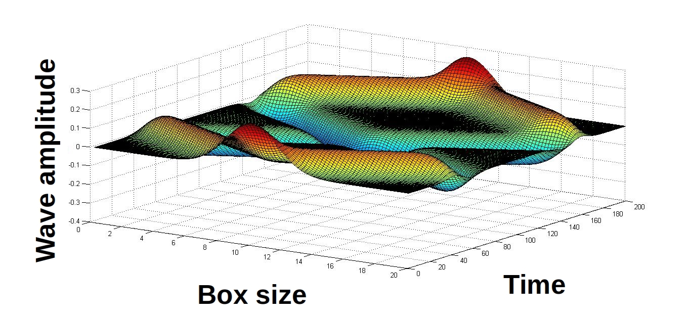
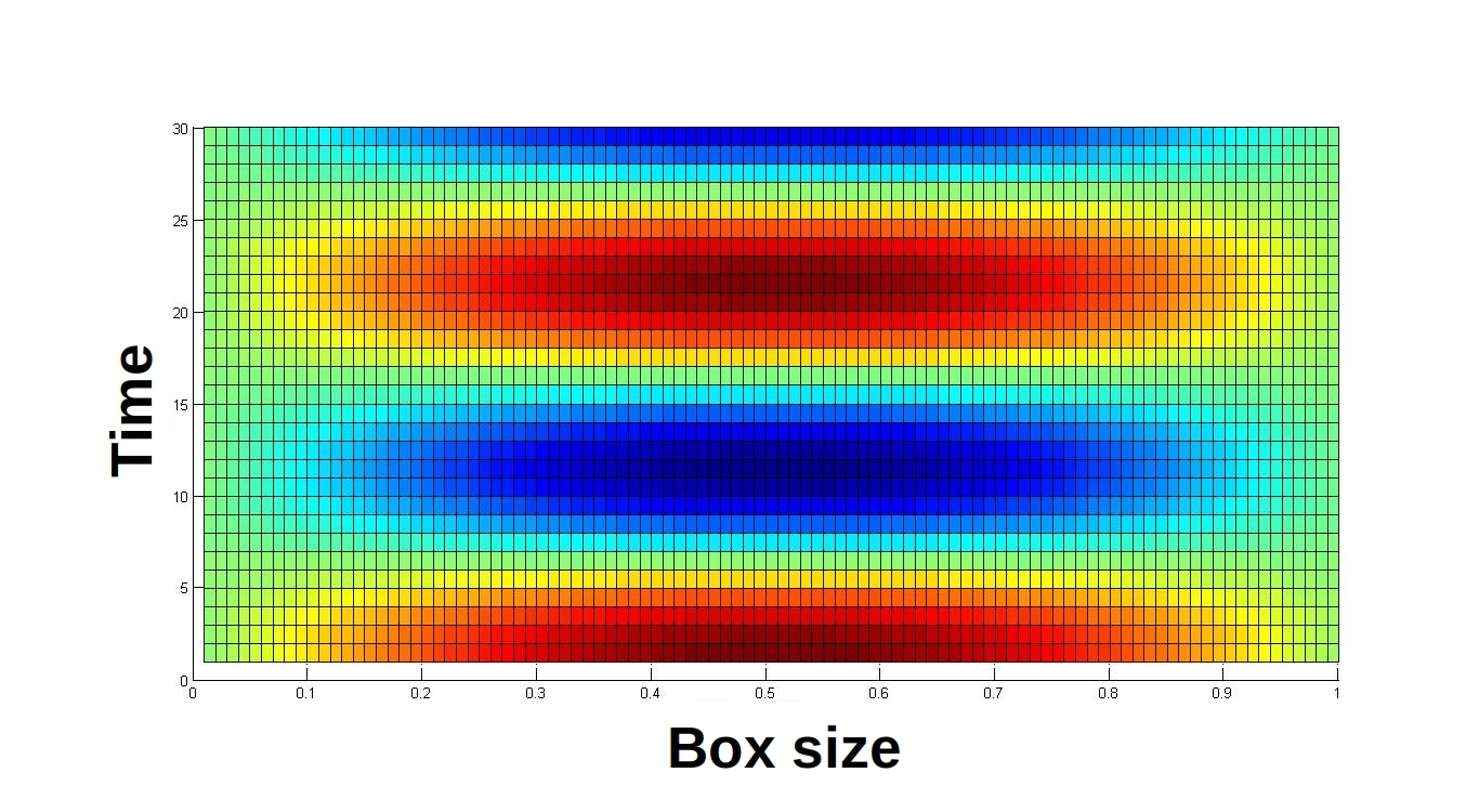
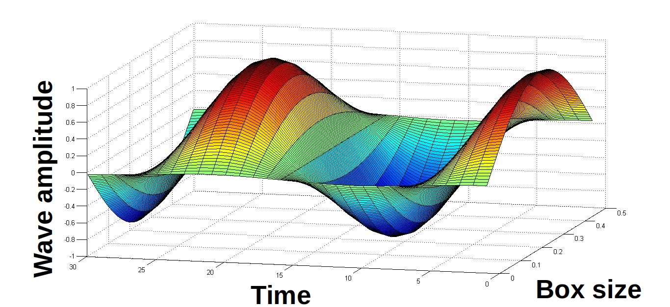
The above analysis can be confirmed by numerical examples, as shown in this section. In all cases one sees that the dynamics and implementation of initial conditions and boundary conditions are consistent with theoretical expectations. Our quantum algorithm is implemented on a gate model quantum computer, and time evolution is discretized into a sequence of elementary gates through the method of [9]. The error induced by this time discretization is rigously upper bounded in [9]. Thus the focus of our numerical study is to investigate the errors induced by spatial discretization and verify the implementation of boundary conditions and initial conditions. To this end, we use the Dormand-Prince method222This is implemented as ODE45 in MATLAB. [13] (a variant of Runge-Kutta) to solve Schrödinger’s equation with Hamiltonians arising from our incidence matrix prescription.
As we know from [14] there is a relation between the timestep and the lattice spacing that is necessary, but not sufficient, to keep the numerical simulations stable, which is
because of that we used this relation in all our numerical analyses.In small examples we verified the accuracy numerical solution to the differential equations by comparing against direct computation of the entire unitary operator applied to the initial state vector.
 |
 |
| a) | b) |
 |
 |
| a) | b) |
 |
 |
| a) | b) |
 a)
a)
|
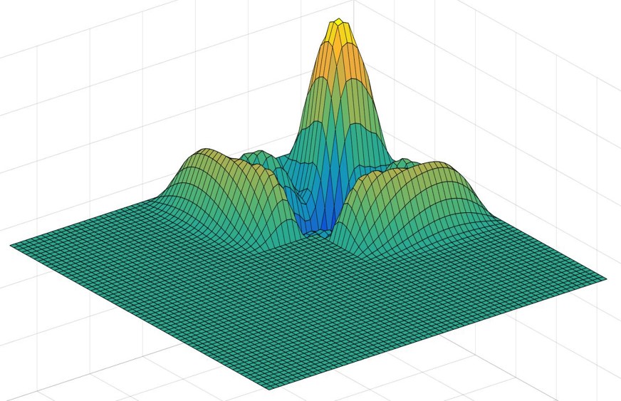 b)
b)
|
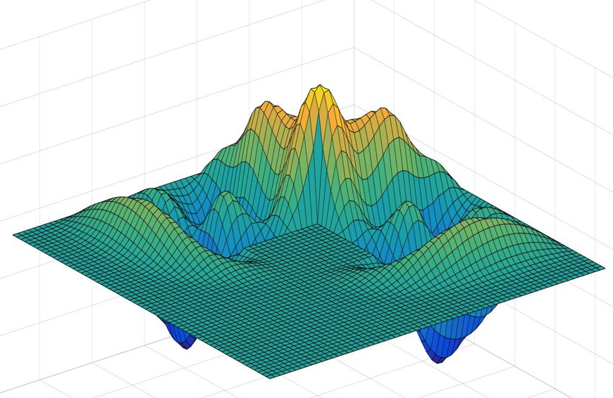 c)
c)
|
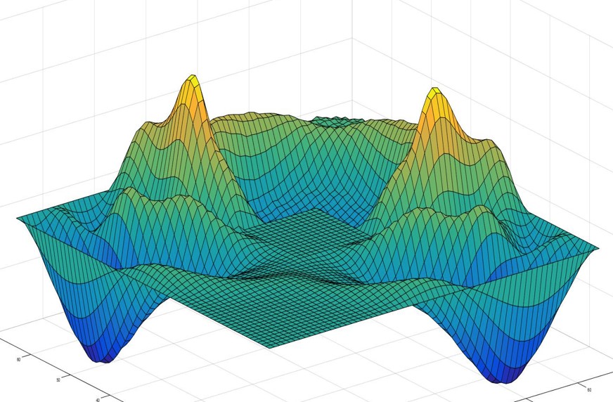 d)
d)
|
6 Higher Order Laplacians
As we have seen, the graph Laplacian is related by a multiplicative constant to the first order approximation of the continuous Laplacian operator; however, higher order approximations might be desired to improve accuracy. In [15] the authors give an expression for a finite difference approximation of the Laplacian operator that is based on the Lagrange interpolation formula and can be taken to arbitrarily high orders of accuracy.
The Lagrange interpolation formula is an exact formula for fitting a polynomial to a set of points . For values of labelled by , the formula is
| (44) |
Taking the second derivative of this formula gives an interpolation formula for an approximation of the Laplace operator. Assuming the values are taken from a uniform lattice (i.e. for ), we can approximate the Laplacian of at using
| (45) |
If we truncate this expression at then we recover the standard second order Laplacian approximation. (Recall that we define order to mean leading error term on a lattice of spacing .)
The next higher order () approximation of is
| (46) |
Assuming the lattice has periodic boundary conditions, then similar formulas hold at points other than . In particular, we can write the fourth order Laplacian for a periodic lattice as
| (47) |
Here is the matrix representation of the cyclic permutation , i.e., it has entries .
7 Boundary Conditions for Higher Order Laplacians
We can accomodate Neumann and Dirichlet boundary conditions by modifying Laplacians for periodic boundary conditions. In particular we follow the algebraic derivation described in Sec. 3.
7.1 Dirichlet Boundary Conditions
As before, we consider a small neighborhood of vertices around . By imposing that for all , we modify the Laplacian as below.
So imposing Dirichlet boundary conditions simply amounts to taking a principal submatrix.
7.2 Neumann Boundary Conditions
To account for Neumann boundary conditions, impose for all . The Laplacian is modified as below.
| (49) | |||||
| (50) | |||||
| (51) | |||||
| (52) |
Note that this is not a symmetric approximation of the Laplacian, not even when restricted to vertices and . However the decoupled second order dynamics of Eqn. 7 require symmetric operators since is Hermitian by construction, so our algorithm cannot use higher order Laplacians for simulating dynamics with Neumann boundary conditions.
7.3 Hypergraph Incidence Matrices
Now that we’ve seen how to impose Dirichlet boundary conditions on higher order Laplacians, we should consider how to generate their incidence matrices. Recall that the fourth order Laplacian with periodic boundary conditions is
which is a sum of circulant matrices. This suggests that a reasonable ansatz for the incidence matrix is . By construction this ansatz has zero sum rows which guarantees that the Laplacian matrix acting on a vector whose entries all have the same value will evaluate to 0 (which is consistent with the fact that the Laplacian operator acting on a constant function evaluates to 0).
From this ansatz we arrive at the following system of degree 2 polynomial equations in and .
| (53) | ||||
| (54) | ||||
| (55) |
Once any two of these is satified the third will also be satisfied since the row sums of the matrix must all be zero. The middle equation gives us , which substituted into the last equation gives which has solutions satisfying . This gives values of and (switching their values gives another solution).
7.4 2 Dimensions and Beyond
The continuous Laplacian in 2 dimensions can be written as , i.e. the sum of the one dimensional Laplacians in the and directions (note that each of these is basis dependent although the total Laplacian is not). Discrete Laplacians in 2 dimensions are similarly constructed.
We discretize space into a square lattice and remove some edges and vertices according to boundary conditions. The resulting graph is a subgraph of the square lattice, so we can separate its edge set into vertical edges, , and horizontal edges, . The subgraphs associated with this partition, and , are composed of several disconnected path graphs (or cycles under periodic boundary conditions). If the lattice is vertices wide and vertices tall then consists of path graphs each on vertices; similarly consists of path graphs each on vertices. If scatterers are introduced then the path graphs composing and will depend on what edges and vertices are removed to account for the scatterers.
Since and are composed of several disconnected path graphs, we can write down their Laplacians and factor them into incidence matrices. The Laplacians and approximate and , respectively, so approximates . If and , then where is the matrix produced by vertically concatenating and .
Generalizing this to -dimensions, the procedure is (1) separate the lattice into graphs (each composed of disconnected paths or cycles) corresponding to each direction in space (2) write down the Laplacians for these graphs and factor them into incidence matrices and (3) vertically concatenate their incidence matrices.
7.5 Sixth (and higher) Order Laplacians
So far our discussion has been restricted to second and fourth order Laplacians; however, we can arrive at higher order Laplacians by (1) taking higher order expansions of the Lagrange interpolation formula, (2) differentiating twice and evaluating at , and (3) reading off the interpolation formula coefficients as matrix coefficients. Periodic boundary conditions are achieved by requiring that the Laplacian be circulant. As before, Dirichlet boundary conditions can be imposed by taking principal submatrices of the Laplacian. Our remarks about generalizing beyond 1-D also hold for higher order Laplacians.
The problem of finding the incidence matrices of higher order Laplacians is a little more involved that in the 1st order case where the graph theoretic interpretation facilitates the factorization. We let denote the radius of a discrete Laplacian. That is, a Laplacian matrix with nonzero entries only out to nearest neighbors has , second nearest neighbors has , and so on. In general the radius Laplacian will be factored into incidence matrices of hypergraphs where each hyperedge can contain up to vertices. (Note: Hyperedges with fewer than vertices will appear if Dirichlet boundary conditions are used.)
As in the and (i.e. second and fourth order) cases, the entries of these incidence matrices can be found by considering the factorization of a Laplacian with periodic boundary conditions. The translational invariance of this case guarantees that all hyperedges will have the same weights and can be oriented identically. Then the entries of the incidence matrix can be found by choosing an appropriate ansatz (one of the form for some and ) and solving the appropriate system of polynomial equations (similar to how 53 was solved). We provide numerical values for the entries of Laplacians and their incidence matrices up to tenth order in appendix C.
8 Discretization Errors
Using a order Laplacian, as described in §6 one expects discretization errors to shrink with lattice spacing as . To obtain a more quantitative assessment of discretization errors, we can numerically compute a metric called the Q factor, which is used to quantify discretization errors in numerical simulations [16].
To compute this factor we use the discretized solutions at three different lattice spacings , and . The Q factor is then defined by
| (56) |
and are defined on different lattices, and thus they are vectors of different dimension. However, we choose the lattices so that the vertices present in the lattice of spacing are a subset of the vertices present in the lattice of spacing . Then, by we really mean the norm of the vector , where is the inclusion map that discards the vector components associated with the vertices absent from the lattice of spacing . For notational simplicity we drop explicit reference to this inclusion map.
Now we want to see the value associated with Eq.(56) when we take the continuum limit, . Straightforward Taylor expansion shows that a order discretized Laplacian, which leaves errors of order should yield a corresponding Q factor of in the limit of going to zero, provided errors from other steps in the algorithm, such as state preparation do not dominate. Now we present a table of values that shows the average of from to , working with as the time step.
| Second order | Fourth order | |
|---|---|---|
| 3.98 | 15.69 | |
| 1.99 | 2.00 | |
| 3.99 | 15.89 |
One sees that for the spreading wave packet case and the standing wave case (both static initial conditions) the Q factors are in good agreement with the expected values of 4 and 16 for the second-order and fourth-order Laplacians. In the case of the rigidly translating wave packet (which corresponds to the initial condition of (31)), the Q factor is approximatly 2 independent of the order of the discretized Laplacian. This is because, in this case, the dominant source of error is in the state preparation. Exact state preparation would involve inverting the incidence matrix, as described in §4.3. The initial state described by (31) is accurate only up to errors of order , thus yielding a Q factor of 2. In appendix B we also obtain an analytical calculation of the Q factor for the special case of a standing wave, treated with a first-order Laplacian.
Since a order Laplacian gives truncation errors of order , the total error accumulated for evolution time will be order . A dimensional Laplacian of order has an incidence matrix which is -sparse; so if an -sparse Hamiltonian is used then . Then the total error accumulated is on the order of .
9 Smoothness
In preceding sections we have discussed the impact of using higher order discretizations to minimize error. In general, both classically and quantumly, one chooses the order of the discretization of the Laplacian on a lattice to obtain discretization errors of order , where is the lattice spacing. The choice of is influenced by the smoothness of the underlying continuum solution that one is attempting to discretize. A high order discretization with error of an derivative is only justified if the exact solution is -times differentiable, since any such discretization of an derivative is derived by Taylor expanding the exact solution to order . Furthermore, knowing the magnitude of these higher derivatives allows quantitative error bounds to be derived, as we show in this section.
Theorem 1.
Let be a bounded convex domain in . Let be a smooth function on that vanishes on the boundaries. Let be the solution to
| (57) |
on with no divergenceless component. Then,
| (58) |
where is the diameter of .
Proof.
The divergence operator is not invertible because it has a kernel. However, it does have a Moore-Penrose pseudoinverse , which is typically expressed in terms of the Green’s function, as follows.
| (59) |
We next note that the Laplacian operator can be written as . (Here, we think of as a column vector of partial derivative operators.) The singular values of the Laplacian are therefore the squares of the singular values of , which is the Divergence operator. The fundamental gap theorem [17, 18] states that on a convex bounded domain , the smallest nontrivial eigenvalue of the Laplacian subject to Neumann boundary conditions is lower bounded by where is the diameter of . Consequently, the smallest nonzero singular value of , i.e. the divergence operator, can be at most . Hence the largest singular value of can be at most . Thus we obtain (58). ∎
Theorem 2.
Let be Hermitian linear combination of finite-order partial derivatives on . Let be the solution to
| (60) |
on some continuous domain subject to Dirichlet or Neumann boundary conditions. We take initial conditions at to be fixed functions , and independent of . Then for any and any
| (61) |
where and
| (62) |
Proof.
Let
| (65) | |||||
| (70) | |||||
| (75) | |||||
| (76) | |||||
| (77) |
By (77),
| (78) | |||||
| (87) |
Thus the solution to (77) satisfies (60). As initial conditions for we can take
| (88) |
where is as defined in (59). By (77) we have
| (89) | |||||
| (90) | |||||
| (91) | |||||
| (92) |
Thus, by the Cauchy-Schwarz inequality
| (93) |
where is a shorthand for . is Hermitian for real and therefore .
| (94) |
Next, we observe that
| (95) |
where the operator
| (96) |
is Hermitian and commutes with . Thus, is conserved, and (94) becomes
| (97) |
which expands out to
| (98) |
By definition
| (99) | |||||
| (100) |
The “Hamiltonians” and are Hermitian so and are time-independent. Thus,
| (101) |
Applying (98) yields
| (102) |
The triangle inequality and (102) yield
In the special case that and is convex we can bound in terms of more accessible quantities, as follows.
Theorem 3.
Let be the solution to
| (105) |
on some convex domain subject to Dirichlet or Neumann boundary conditions. We take initial conditions at to be fixed functions , and independent of . Then for any and any
| (106) |
where .
Proof.
Theorem 2 gives a very nice quantitative upper bound on discretization errors in terms of directly accessible properties of the initial conditions. However, it only applies under the specific condition that the error term of interest is expressible as a negative coefficient times the square of a Hermitian linear combination of partial derivatives. Not all discretized Laplacians satisfy this. However, it is possible to engineer high order Laplacians such that this is the case. We illustrate this by giving an explicit discretized Laplacian in two dimensions with error of order , which satisfies this condition. The formula is
| (112) |
as one can verify by Taylor expansion. Thus “stencil” for discretizing a two dimensional Laplacian is illustrated in figure 7. An incidence matrix factorization for this stencil-based Laplacian is given in appendix C.3.
Theorem 3 has the benefit that the error bound is characterized directly in terms of easily accessible quantities ( and ). However, the downside is that the condition on the error term (namely that it should take the form of a negative coefficient times the square of a Laplacian) is somewhat restrictive. Theorem 2 is more general in that the error term could be higher order, but still requires it to be the square of a differential operator. In appendix A we derive an alternative theorem which relaxes this restriction and can be applied to Laplacians that are constructed directly as a sum of discretized second partial derivatives. Relative to stencil-based discrete Laplacians such as in figure 7 these Laplacians are much easier to derive and factor into incidence matrices at any order. On the other hand, we do not know how to use the methods of appendix A appears to obtain an error bound directly in terms of and . (In other words, appendix A contains only an analogue of theorem 2 but no analogue of theorem 3.) We include both versions of our analysis as we believe it may depend on context which one is more useful. A related question, which we leave for future work, is whether the specialized forms for the discretized Laplacians devised in this section and in appendix A result in smaller discretization errors than other discretized Laplacians at the same order. It is quite possible that they only aid in yielding provable error bounds but do not actually yield smaller error in practice.

10 Post-Processing
After performing Hamiltonian simulation we are left with a state which encodes both and . Depending on the application, we might be interested in just or just or both.
If our goal is to produce a state proportional to then the post-processing amounts to measuring if the state is in or (recall the full Hilbert space is ), with success if it is measured in . In general we cannot give a reasonable lower bound on the success probability of this measurement, even for simple systems. To see this, consider the case of the standing wave in 1D with Dirichlet boundary conditions. The initial conditions are and , and at any other time the field can be written for some that oscillates between 1 and -1. If the evolution time is chosen so that then . So the state will have no support (up to errors from the finite difference method) in . However, at least in this example, for average choice of instead of worst-case, one will have an probability of obtaining the subspace. The same issue arises if we are instead wish to extract from the complementary subspace.
If our goal is to produce a state proportional to then the post-processing is a little more complicated. We begin by measuring if the state is in or , with success if it is measured in . The resulting state is proportional to , so it remains to cancel . This inverse can be canceled in much the same way that was originally applied. Mirroring the procedure for matrix inversion in [7], the procedure for matrix multiplication is
| (113) | ||||
| (114) | ||||
The first line re-expresses the initial state in the eigenbasis of the Hamiltonian which is simulated in the subsequent phase estimation step.
In the second line we run phase estimation on the unitary , where is exactly the same Hamiltonian we used for simulating the wave equation, and write the eigenvalues to the second register. We use to denote the eigenstate with eigenvalue , but we use to denote a state encoding the approximation of the eigenvalue output by phase estimation.
In the third line we perform a controlled rotation of the second qubit. The constant must satisfy so that the argument under the square root is not negative. Setting it to , the probability of measuring the last qubit in is in the worst case (i.e. when the initial state only has support in the ground space of the Hamiltonian.). Then we produce a state proportional to conditioned on measuring the last qubit in the state .
11 Comparison to Other Quantum Algorithms
As discussed in the introduction, there are three quantum algorithms to which ours can be meaningfully compared. The algorithm of Clader, Jacobs, and Sprouse solves a problem related to, but not identical with, that solved here. Namely they give a quantum algorithm to compute scattering crossections in the special case of monochromatic illumination [5]. In [6], Montanaro and Pallister analyze the degree to which quantum linear system algorithms can achieve speedups for finite element methods. The performance of such quantum algorithms when applied to wave equations is a complex question that we defer to future work.
The most direct comparison to our algorithm can be made with the algorithm of Berry, Childs, Ostrander, and Wang [2]. Since the algorithm of [2] only works for first order differential equations, we must introduce ancillary variables to simulate a second order differential equation. To simulate the wave equation for , we introduce the variable , in which case we have the first order equation
| (115) |
Let
| (116) |
and let be a matrix that diagonalizes :
| (117) |
( is defined only up to an overal normalization.) The complexity of the algorithm of [2] is dictated by , the condition number of (which is independent of the normalization of ). Specifically, theorem 9 of [2] gives a runtime upper bound for their quantum algorithm of
| (118) |
where is the sparsity of , and is a measure of how much the norm of the solution vector varies over the duration of the simulation, namely
| (119) |
We can see that for the problem at hand, as the lattice spacing is taken to zero:
| (120) |
We can work out by noting that is diagonalized by the matrix whose columns are the eigenvectors of . That is, if the eigenvectors of are with corresponding eigenvalues then where
| (121) |
Let denote the eigenvectors of . By inspecting (116) one sees that the eigenvectors of are
| (122) |
( is the dimension of and is the dimension of .)
We can thus write in the following block form.
| (123) |
where
| (124) |
and
| (125) |
is a symmetric matrix so form an orthogonal basis. We choose the normalizations to make it orthonormal. Let be the orthogonal matrix that diagonlizes . Then
| (126) |
where
| (127) |
Permuting the basis then yields
| (128) |
where for each the block is given by the following matrix
| (129) |
This preceeding manipulations were all changes of basis, which do not affect the eigenspectrum of. Thus, the eigenvalues of are the eigenvalues of . By direct calculation, the eigenvalues of are and where
| (130) |
For a path graph of vertices the eigenvalues of the Laplacian range from to , and the same is true for any larger constant number of dimensions for the eigenvalues of an grid. The smallest eigenvalue of is thus with where indexes the smallest eigenvalue of . Thus, for large , we can approximate by Taylor expanding to lowest order in , obtaining
| (131) | |||||
| (132) |
which is of order . Similarly, we can see that the largest eigenvalue of is and thus
| (133) |
Substituting (133) and (11) into (118) yields a total complexity of for the quantum algorithm of [2].
In the algorithm presented here, we have quadratically better dependence on . There are three places for this dependence to come into the total complexity of our algorithm. First, if we choose to prepare an arbitrary initial state, then the first step of our algorithm is to implement, via quantum linear algebra methods [7, 8, 19] the Moore-Penrose pseudoinverse of the incidence matrix . The complexity of this step is proportional to the condition number of , which is the square root of the condition number of the Laplacian 333The condition numbers of and will both depend on the connectivity of the lattice. These condition numbers can be large if scatterers are present which create bottlenecks in the lattice, i.e., convex locations where only a few edges can be removed that will partition the lattice into two relatively large components.. A second place that the condition number can contribute to the complexity is in the post-processing, as we saw when we considered producing a state proportional to . Here our approach also scales quadratically better with respect to the condition number of the Laplacian. Additionally, the number of qubits required by our algorithm is where is the number of lattice sites, whereas the number of qubits required by the algorithm of [2] is , where is the duration of the process to be simulated.
It is worthwhile to relate the Laplacian’s condition number, which is a fairly abstract quantity, with parameters of more direct physical significance. In the case of a Laplacian for a -dimensional cubic volume of dimension discretized into a cubic lattice of spacing one sees that the largest eigenvalue of is of order and the smallest eigenvalue is of order . Thus the condition number of the Laplacian is of order , so the incidence matrix has a condition number of order . In our algorithm, the simulation of the time-evolution itself, achieved using [9], scales as . Thus, both state preparation and time-evolution have complexity scaling linearly in .
12 Klein-Gordon Equation
Going to relativistic theories we know that spinless particles are described by the Klein-Gordon equation,
| (134) |
where is the particle mass, is the speed of light and the Planck constant. In order to not carry these constants any more we will adopt the natural units, which implies and .
As we can see we are dealing with a wave equation, and thus it also should admit some Hamiltonian in our Schrödinger equation. Suppose we have a graph , where
is the discretized version of Eq.(134). It means that our Laplacian has the whole information about the particle, which includes its mass term. In fact this graph can be easily achieved from a graph that gives our ordinary wave equation, which means does not have a mass term.
Starting with the mass term can be realized by adding self loops with as its weight on all vertices of . This manipulated graph is our graph . Finally, as we did before, we need to construct its incidence matrix in order to get the Laplacian,
Besides, without difficult we can see how this Laplacian is related with the Laplacian from
where is the identity matrix. Therefore, whereas gives our ordinary wave equation, applying in our Hamiltonian gives our relativistic wave equation.
13 Maxwell’s Equations
With and without sources, Maxwell’s equations governing the time evolution of electric and magnetic fields take the form
which imply that and both follow the wave equation. If we consider discretizing space, then we can write these as
where is the finite difference approximation of the curl operator. To see how to construct , consider the following
This suggests we should consider the linear differential equation
| (135) |
We can discretize space into a uniform cubic lattice and approximate the differential operators using finite difference methods to reduce this to an ordinary differential equation. (Appendix C contains numerical values for the entries of these operators up to tenth order.) This ordinary differential equation will be a case of Schrödinger’s equation since the approximate differential operators coming from the Lagrange interpolation formula are anti-Hermitian. In this case, unitarity translates to conservation of the classical energy contained in the field .
14 Future Work
It is an interesting open question whether our quantum algorithm is optimal. In particular, it is natural to ask whether an analogue of the no-fast-forwarding theorem from [20] could yield a lower bound for the complexity of the problem of simulating wave equations that matches the complexity of the algorithm presented here. It is also interesting to investigate the performance of quantum algorithms for simulating the wave equation based on finite element methods, rather than finite difference methods, as considered here. Another direction for future work is to use automated circuit synthesis techniques to generate concrete quantum circuits implementing our algorithm and thereby obtain quantitative resource estimates for benchmark instances of wave equation simulation problems. Lastly, one can consider extending the quantum algorithm presented here to more complicated wave equations.
15 Acknowledgements
The authors thank Yi-Kai Liu and Eite Tiesinga for insightful discussions. The authors also thank David Gosset, Gorjan Alagic, Peter Bierhorst, and anonymous referees for useful feedback on the manuscript. This research was supported by the Department of Energy under award number DE-SC0016431. Parts of this research were completed while SJ was an employee of the National Institute of Standards and Technology, an agency of the US government. The resulting portions of this manuscript are not subject to US copyright.
Appendix A Alternative Smoothness Analysis
Theorem 4.
Let be the solution to
| (136) |
on some compact continuous domain subject to some specified boundary conditions. We take initial conditions at to be fixed functions and independent of . Then for any and any
where and
| (137) |
Proof.
Let
| (141) | |||||
| (142) | |||||
| (143) | |||||
| (147) | |||||
| (151) | |||||
| (152) | |||||
| (153) |
By (153),
| (154) | |||||
| (161) |
Thus the solution to (153) satisfies (136). As initial conditions for we take
| (162) | |||||
| (163) |
where is as defined in (59). By (153) we have
| (164) | |||||
| (165) | |||||
| (166) | |||||
| (167) |
Thus, by the Cauchy-Schwarz inequality
| (168) |
where is a shorthand for . is Hermitian for real and therefore . Thus (168) simplifies to
| (169) |
Next, observe that
| (170) |
and
| (171) | |||||
| (172) |
where
| (173) |
For any , commutes with the and is Hermitian. Thus
| (174) |
Next, we observe that
| (175) | |||||
| (176) | |||||
| (177) |
where
| (178) |
is Hermitian and commutes with thus, by (163),
| (179) |
Substituting these results into (170) yields
| (180) |
Substituting (180) into (169) yields
| (181) |
By definition
| (182) | |||||
The “Hamiltonians” and are Hermitian so and are time-independent for any . Thus,
| (183) |
Thus, by (181)
| (184) |
By the triangle inequality
The initial conditions have , and therefore
| (186) |
Applying (184) to (186) yields
| (187) |
Recalling the definition of (141),
| (188) |
Thus (186) implies the bound
| (189) |
By (173), (141), and (163), (189) becomes
∎
Theorem 4 gives a very nice quantitative upper bound on discretization errors in terms of directly accessible properties of the initial conditions. Furthermore, theorem 1 shows that the quantity has magnitude not too much larger than the chosen initial velocity . However, theorem 4 applies only under the specific condition that the error term of interest is expressible as a positive coefficient times the sum of derivatives. Not all discretized Laplacians satisfy this. However, it is possible to engineer high order Laplacians such that this is the case. This problems reduces to engineering a high order discretized one-dimensional derivatives such that the leading error term is a positive coefficient times an even derivative. The Laplacian in dimensions can then be composed as the sum of these discretized derivatives along each of the coordinate axes.
We illustrate this by giving an explicit discretized Laplacian in one dimension with error of order , which satisfies this condition and then computing a corresponding incidence matrix factorization. By Taylor expansion, one can verify that
| (190) | |||||
On a one dimensional lattice with periodic boundary conditions we can write this Laplacian as
where is the cyclic shift operator and
Next, we verify that this can be factorized as
| (191) |
with sparse . To this end we introduce the ansatz
| (192) |
The requirement (191) then determines a system of quadratic equations constraining . One solution to this system of equations is (up to 6 digits of precision)
as one can verify.
Appendix B Analytical Q
We begin by giving the mesh spacing as a function of the number of vertices for our one dimensional lattice
| (193) |
As discussed in §8, in order to get we need to work with the three different mesh spacing , and , where the relation between them can be established working with the follow total number of vertices
| (194) | |||||
respectively. Moving forward we get three discrete functions that describe the standing wave,
| (195) | |||||
where is the frequency of the wave,
| (196) | |||||
From the factor definition we know that we need to compute two differences and . However, these points should be computed at the same distance, which means , and . Let us proceed with the follow computation,
But we are interest in the continuum limit of this expression, with means or . Thus, from now the idea is to work with approximate values. Starting with the frequency,
where
and
Now we can use the following trigonometric property,
with
But for large we get the follow approximations
However, our real interest is computing the norm in the continuum limit,
where we can make use of the expression below,
Therefore,
Similarly, for we get
Thus, combining these two results in the Q factor expression we establish
that agrees with the value for in the Richardson expansion and with our numerical result.
The same steps can be done for the second order Laplacian to see in the continuum limit. However the correct wave frequency for this case is
Appendix C Numerical Values for Higher Order Operators
In this appendix we provide tables of numerical values for the entries of higher order approximations of derivative operators, specifically the first derivative and the Laplacian. We also include a table of values for factorizing higher order Laplacians, and we discuss how to deal with factorizing stencil based Laplacians in more than one dimension. We use order to indicate that at lattice spacing , the leading error term in the discrete derivative is of order .
C.1 First Derivative
Below is a table of numerical values used for higher order approximations of the first-order derivative. For a 1D space with periodic boundary conditions, the radius- approximation is where represents a cyclic permutation of the vertices, i.e., for .
operator
radius
order
entries to
1
2
-1/2, 0 ,1/2
2
4
1/12, -2/3, 0, 2/3, -1/12
3
6
-1/60, 3/20, -3/4, 0, 3/4, -3/20, 1/60
4
8
1/280, -4/105, 1/5, -4/5, 0, 4/5, -1/5, 4/105, -1/280
5
10
-1/1260, 5/504, -5/84, 5/21, -5/6, 0, 5/6, -5/21, 5/84, -5/504, 1/1260
C.2 1-D Laplacians
If we take the second derivative of the Lagrange interpolation formula (truncated at the -th order), we arrive at Eqn. 45. Using this expression, we can find the coefficients which let us write the Laplacian under periodic boundary conditions as . Since the Laplacian is symmetric . In the table below we give the values for for the first 5 orders of truncation.
operator
radius
order
to
1
2
-2,1
2
4
-5/2,4/3,-1/12
3
6
-49/18,3/2,-3/20,1/90
4
8
-205/72,8/5,-1/5,8/315,-1/560
5
10
-5269/1800,5/3,-5/21,5/126,-5/1008,1/3150
In order to implement our algorithm using any of the above Laplacians, we need to know its incidence matrix factorization. A simple procedure for doing this is the following:
-
1.
Generate the coefficients of the Laplacian operator using the Lagrange interpolation formula.
-
2.
With these coefficients, write the Laplacian for a 1-D grid with periodic boundary conditions in the form . Note since Laplacians are symmetric.
-
3.
Build an ansatz for the incidence matrix of the form .
-
4.
Calculate .
-
5.
Solve for the values .
We choose the ansatz instead of one like so that automatically has zero sum rows and columns like a Laplacian under periodic boundary conditions. The table below gives values for which lead to various higher order Laplacians.
| radius | to |
|---|---|
| 1 | 1 |
| 2 | 1.1547, - (0.5774 0.5) |
| 3 | 1.2192, -0.1247, 0.0101 |
| 0.1247, -1.2192, 1.1046 | |
| 4 | -0.0465, 1.1508, -1.2284, 0.1076 |
| 1.2540, -0.1552, 0.0209, -0.0016 | |
| 0.0209, -0.1552, 1.2540, -1.1181 | |
| 1.2284, -1.1508, 0.0465, -0.0166 | |
| 5 | -0.0041, 0.0306, -0.1762, 1.2756, -1.1262 |
| 1.2756, -0.1762, 0.0306,-0.0041,0.0003 | |
| 0.0289, 1.0626, -1.3223, 0.2195, -0.0131 | |
| 0.2195, -1.3223, 1.0626, 0.02891, 0.0243 |
C.3 2-D Laplacians
If we restrict to decomposing Laplacians into the form (treating the total Laplacian operator as the sum of the Laplacians in the and directions) then we can factor them simply by concatenating incidence matrices, as described in Subsection 7.4. These Laplacians are a restricted case since they approximate the second derivative at vertex using only the values of the function at vertices in the set (i.e. using vertices lying on a -sign shaped subset of the vertices at distance from ).
Another well-known way to approximate Laplacians in multiple dimensions is to use stencils such as the one in Figure 7. These have the disadvantage that their incidence matrices are not simply the concatenation of incidence matrices for Laplacians in the and directions; however, our procedure for calculating incidence matrix factorizations in this case can generalize. Using stencils has the advantage that they approximate the Laplacian at using all points within some distance of and not just those within distance in the of direction.
We show how to factor the Laplacian corresponding to the stencil in Fig. 7 which has error of order . The formula is
| (197) |
as one can verify by Taylor expansion. Previously we assumed we worked in a large one dimensional space with periodic boundary conditions; in this case we assume we’re working on a large 2D space with periodic boundaries which can be treated as a torus discretized using a square grid. The Laplacian matrix can then be expressed as
Our ansatz for the incidence matrix is
where denotes the horizontal concatenation of matrices and . By construction this ansatz has zero-sum rows.
In terms of hypergraphs, this incidence matrix has hyperedges connecting vertices at distance at most from each other, so the stencil they produce will have diameter at most . In fact there are two types of hyperedges present. Those encoded in the left block of the incidence matrix (the part where the coefficients appear) are hyperedges which span all neighbors of their center vertices; those encoded in the right block span all neighbors of their center vertex which have the same coordinate.
The stencil in Figure 7 has diameter 4, and to factor it it suffices to set . Doing so we find 16 solutions for the coefficients and , one of which is
| (199) |
One might expect to find solutions with for all ; however, they don’t exist. This reveals the importance of choosing the right ansatz for an incidence matrix factorization. For example, when factoring a 3D Laplacian built from a stencil with diameter , one might try the ansatz
and not find solutions, while the ansatz
might have solutions.
References
- [1] Dominic W Berry. High-order quantum algorithm for solving linear differential equations. Journal of Physics A: Mathematical and Theoretical, 47(10):105301, 2014.
- [2] Dominic W. Berry, Andrew M. Childs, Aaron Ostrander, and Guoming Wang. Quantum algorithm for linear differential equations with exponentially improved dependence on precision. Communications in Mathematical Physics, 356(3):1057–1081, Dec 2017.
- [3] Sarah K Leyton and Tobias J Osborne. A quantum algorithm to solve nonlinear differential equations. arXiv preprint arXiv:0812.4423, 2008.
- [4] Yudong Cao, Anargyros Papageorgiou, Iasonas Petras, Joseph Traub, and Sabre Kais. Quantum algorithm and circuit design solving the poisson equation. New Journal of Physics, 15(1):013021, 2013.
- [5] B. D. Clader, B. C. Jacobs, and C. R. Sprouse. Preconditioned quantum linear system algorithm. Phys. Rev. Lett., 110:250504, Jun 2013.
- [6] Ashley Montanaro and Sam Pallister. Quantum algorithms and the finite element method. Phys. Rev. A, 93:032324, Mar 2016.
- [7] Aram W. Harrow, Avinatan Hassidim, and Seth Lloyd. Quantum algorithm for linear systems of equations. Phys. Rev. Lett., 103:150502, Oct 2009.
- [8] Andrew M. Childs, Robin Kothari, and Rolando D. Somma. Quantum algorithm for systems of linear equations with exponentially improved dependence on precision. SIAM Journal on Computing, 46(6):1920–1950, Jan 2017.
- [9] D. W. Berry, A. M. Childs, and R. Kothari. Hamiltonian simulation with nearly optimal dependence on all parameters. In 2015 IEEE 56th Annual Symposium on Foundations of Computer Science, pages 792–809, Oct 2015.
- [10] Lov K. Grover. Synthesis of quantum superpositions by quantum computation. Phys. Rev. Lett., 85:1334–1337, Aug 2000.
- [11] Christof Zalka. Efficient simulation of quantum systems by quantum computers. Fortschritte der Physik, 46:877–879, 1998.
- [12] Lov Grover and Terry Rudolph. Creating superpositions that correspond to efficiently integrable probability distributions. arXiv preprint quant-ph/0208112, 2002.
- [13] J.R. Dormand and P.J. Prince. A family of embedded runge-kutta formulae. Journal of Computational and Applied Mathematics, 6(1):19 – 26, 1980.
- [14] Lax P. D. and Ichtmyer R. D. R. Survey of the stability of linear finite difference equations. Communications on Pure and Applied Mathematics, 9:267–293, May 1956.
- [15] Colbert Daniel T. and Miller William H. A novel discrete variable representation for quantum mechanical reactive scattering via the s-matrix kohn method. The Journal of chemical physics, 96:1982–1991, 1992.
- [16] Choptuik Matthew W. Lectures for VII Mexican School on Gravitation and Mathematical Physics; Relativistic and Numerical Relativity; Numerical Analysis for Numerical Relativists. University of British Columbia, 2009.
- [17] Payne L. E. and Weinberger H. F.
- [18] Andrews Ben and Clutterbuck Julie. Proof of the fundamental gap conjecture. Journal of the Americal Mathematical Society, 24:899–916, Mar 2011.
- [19] Ambainis Andris. Variable time amplitude amplification and faster quantum algorithm for solving systems of linear equations. arXiv:1010.4458 [quant-ph], 2012.
- [20] Dominic W. Berry, Graeme Ahokas, Richard Cleve, and Barry C. Sanders. Efficient quantum algorithms for simulating sparse hamiltonians. Communications in Mathematical Physics, 270(2):359–371, Mar 2007.