FarmTest: Factor-adjusted robust multiple testing
with approximate false discovery control

Abstract

Large-scale multiple testing with correlated and heavy-tailed data arises in a wide range of research areas from genomics, medical imaging to finance. Conventional methods for estimating the false discovery proportion (FDP) often ignore the effect of heavy-tailedness and the dependence structure among test statistics, and thus may lead to inefficient or even inconsistent estimation. Also, the commonly imposed joint normality assumption is arguably too stringent for many applications. To address these challenges, in this paper we propose a Factor-Adjusted Robust Multiple Testing (FarmTest) procedure for large-scale simultaneous inference with control of the false discovery proportion. We demonstrate that robust factor adjustments are extremely important in both controlling the FDP and improving the power. We identify general conditions under which the proposed method produces consistent estimate of the FDP. As a byproduct that is of independent interest, we establish an exponential-type deviation inequality for a robust $U$-type covariance estimator under the spectral norm. Extensive numerical experiments demonstrate the advantage of the proposed method over several state-of-the-art methods especially when the data are generated from heavy-tailed distributions. The proposed procedures are implemented in the R-package FarmTest.

Keywords: Factor adjustment; False discovery proportion; Huber loss; Large-scale multiple testing; Robustness.

1 Introduction

Large-scale multiple testing problems with independent test statistics have been extensively explored and is now well understood in both practice and theory (Benjamini and Hochberg, 1995; Storey, 2002; Genovese and Wasserman, 2004; Lehmann and Romano, 2005). Yet, in practice, correlation effects often exist across many observed test statistics. For instance, in neuroscience studies, although the neuroimaging data may appear very high dimensional (with millions of voxels), the effect degrees of freedom are generally much smaller, due to spatial correlation and spatial continuity (Medland et al., 2014). In genomic studies, genes are usually correlated regulatorily or functionally: multiple genes may belong to the same regulatory pathway or there may exist gene-gene interactions. Ignoring these dependence structures will cause loss of statistical power or lead to inconsistent estimates.

To understand the effect of dependencies on multiple testing problems, validity of standard multiple testing procedures have been studied under weak dependencies, see Benjamini and Yekutieli (2001), Storey (2003), Storey et al. (2004), Ferreira and Zwinderman (2006), Chi (2007), Wu (2008), Clarke and Hall (2009), Blanchard and Roquain (2009) and Liu and Shao (2014), among others. For example, it has been shown that, the Benjamini-Hochberg procedure or Storey’s procedure, is still able to control the false discovery rate (FDR) or false discovery proportion, when only weak dependencies are present. Nevertheless, multiple testing under general and strong dependence structures remains a challenge. Directly applying standard FDR controlling procedures developed for independent test statistics in this case can lead to inaccurate false discovery control and spurious outcomes. Therefore, correlations must be accounted for in the inference procedure; see, for example, Owen (2005), Efron (2007, 2010), Leek and Storey (2008), Sun and Cai (2009), Friguet et al. (2009), Schwartzman and Lin (2011), Fan et al. (2012), Desai and Storey (2012), Wang et al. (2017) and Fan and Han (2017) for an unavoidably incomplete overview.

In this paper, we focus on the case where the dependence structure can be characterized by latent factors, that is, there exist a few unobserved variables that correlate with the outcome. A multi-factor model is an effective tool for modeling dependence, with wide applications in genomics (Kustra et al., 2006), neuroscience (Pournara and Wernish, 2007) and financial economics (Bai, 2003). It relies on the identification of a linear space of random vectors capturing the dependence structure of the data. In Friguet et al. (2009) and Desai and Storey (2012), the authors assumed a strict factor model with independent idiosyncratic errors, and used the EM algorithm to estimate the factor loadings as well as the realized factors. The FDP is then estimated by subtracting out the realized common factors. Fan et al. (2012) considered a general setting for estimating the FDP, where the test statistics follow a multivariate normal distribution with an arbitrary but known covariance structure. Later, Fan and Han (2017) used the POET estimator (Fan et al., 2013) to estimate the unknown covariance matrix, and then proposed a fully data-driven estimate of the FDP. Recently, Wang et al. (2017) considered a more complex model with both observed primary variables and unobserved latent factors.

All the methods above assume joint normality of factors and noise, and thus methods based on least squares regression, or likelihood generally, can be applied. However, normality is really an idealization of the complex random world. For example, the distribution of the normalized gene expressions is often far from normal, regardless of the normalization methods used (Purdom and Holmes, 2005). Heavy-tailed data also frequently appear in many other scientific fields, such as financial engineering (Cont, 2001) and biomedical imaging (Eklund et al., 2016). In finance, the seminal papers by Mandelbrot (1963) and Fama (1963) discussed the power law behavior of asset returns, and Cont (2001) provided extensive evidence of heavy-tailedness in financial returns. More recently, in functional MRI studies, it has been observed by Eklund et al. (2016) that the parametric statistical methods failed to produce valid clusterwise inference, where the principal cause is that the spatial autocorrelation functions do not follow the assumed Gaussian shape. The heavy-tailedness issue may further be amplified by high dimensionality in large-scale inference. In the context of multiple testing, as the dimension gets larger, more outliers are likely to appear, and this may lead to significant false discoveries. It is therefore imperative to develop inferential procedures that adjust dependence and are robust to heavy-tailedness at the same time.

In this paper, we investigate the problem of large-scale multiple testing under dependence via an approximate factor model, where the outcome variables are correlated with each other through latent factors. To simultaneously incorporate the dependencies and tackle with heavy-tailed data, we propose a factor-adjusted robust multiple testing (FarmTest) procedure. As we proceed, we gradually unveil the whole procedure in four steps. First, we consider an oracle factor-adjusted procedure given the knowledge of the factors and loadings, which provides the key insights into the problem. Next, using the idea of adaptive Huber regression (Zhou at al., 2018; Sun et al., 2017), we consider estimating the realized factors when the loadings were known and provide a robust control of the FDP. In the third part, we propose two robust covariance matrix estimators, a $U$-statistic based estimator and another one based on elementwise robustification. We then apply spectral decomposition to these estimators and use principal factors to recover the factor loadings. The final part, which is provided in Appendix A, gives a fully data-driven testing procedure based on sample splitting: use part of the data for loading construction and the other part for simultaneous inference.

Figure 1: Histograms of four different mean estimators for simultaneous inference.

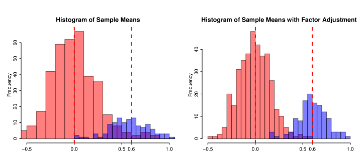
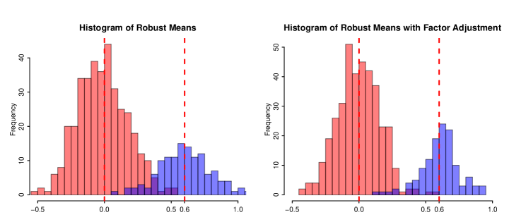
First we illustrate our methodology with a numerical example that consists of observations $\bm{X}_{i}$’s generated from a three-factor model:

$$\bm{X}_{i}=\bm{\mu}+\mathbf{B}\bm{f}_{i}+\bm{\varepsilon}_{i},~{}~{}~{}i=1,\ldots,n,$$

where $\bm{f}_{i}\sim\mathcal{N}(\textbf{0},\mathbf{I}_{3})$ and the entries of $\mathbf{B}$ are independent and identically distributed (IID) from a uniform distribution, $\mathcal{U}(-1,1)$. The idiosyncratic errors, $\bm{\varepsilon}_{i}$’s, are independently generated from the $t_{3}$-distribution with 3 degrees of freedom. The sample size $n$ and dimension $p$ are set to be $100$ and $500$, respectively. We take the true means to be $\mu_{j}=0.6$ for $1\leq j\leq 0.25\times p$ and $0$ otherwise. In Figure 1, we plot the histograms of sample means, robust mean estimators, and their counterparts with factor-adjustment. Details of robust mean estimation and the related factor-adjusted procedure are specified in Sections 2 and 3. Due to the existence of latent factors and heavy-tailed errors, there is a large overlap between sample means from the null and alternative, which makes it difficult to distinguish them from each other. With the help of either robustification or factor-adjustment, the null and alternative are better separated as shown in the figure. Further, with both factor-adjustment and robustification, the resulting estimators are tightly concentrated around the true means so that the signals are evidently differentiated from the noise. This example demonstrates the effectiveness of the factor-adjusted robust multiple testing procedure.

The rest of the paper proceeds as follows. In Section 2, we describe a generic factor-adjusted robust multiple testing procedure under the approximate factor model. In Section 3, we gradually unfold the proposed method, while we establish its theoretical properties along the way. Section 4 is devoted to simulated numerical studies. Section 5 analyzes an empirical dataset. We conclude the paper in Section 6. Proofs of the main theorems and technical lemmas are provided in the online supplement.

Notation. We adopt the following notations throughout the paper. For any $d\times d$ matrix $\mathbf{A}=(A_{k\ell})_{1\leq k,\ell\leq d}$, we write $\|\mathbf{A}\|_{\max}=\max_{1\leq k,\ell\leq d}|A_{k\ell}|$, $\|\mathbf{A}\|_{1}=\max_{1\leq\ell\leq d}\sum_{k=1}^{d}|A_{k\ell}|$ and $\|\mathbf{A}\|_{\infty}=\max_{1\leq k\leq d}\sum_{\ell=1}^{d}|A_{k\ell}|$. Moreover, we use $\|\mathbf{A}\|$ and ${\rm tr}(\mathbf{A})=\sum_{k=1}^{d}A_{kk}$ to denote the spectral norm and the trace of $\mathbf{A}$. When $\mathbf{A}$ is symmetric, we have $\|\mathbf{A}\|=\max_{1\leq k\leq d}|\lambda_{k}(\mathbf{A})|$, where $\lambda_{1}(\mathbf{A})\geq\lambda_{2}(\mathbf{A})\geq\cdots\geq\lambda_{d}(\mathbf{A})$ are the eigenvalues of $\mathbf{A}$, and it holds $\|\mathbf{A}\|\leq\|\mathbf{A}\|_{1}^{1/2}\|\mathbf{A}\|_{\infty}^{1/2}\leq\max\{\|\mathbf{A}\|_{1},\|\mathbf{A}\|_{\infty}\}\leq d^{1/2}\|\mathbf{A}\|$. We use $\lambda_{\max}(\mathbf{A})$ and $\lambda_{\min}(\mathbf{A})$ to denote the maximum and minimum eigenvalues of $\mathbf{A}$, respectively.

2 FarmTest

In this section, we describe a generic factor-adjusted robust multiple testing procedure under the approximate factor model.

2.1 Problem setup

Let $\bm{X}=(X_{1},\ldots,X_{p})^{\mathrm{\scriptstyle T}}$ be a $p$-dimensional random vector with mean $\bm{\mu}=(\mu_{1},\ldots,\mu_{p})^{\mathrm{\scriptstyle T}}$ and covariance matrix $\bm{\Sigma}=(\sigma_{jk})_{1\leq j,k\leq p}$. We assume the dependence structure in $\bm{X}$ is captured by a few latent factors such that $\bm{X}=\bm{\mu}+\mathbf{B}\bm{f}+\bm{\varepsilon}$, where $\mathbf{B}=(\bm{b}_{1},\ldots,\bm{b}_{p})^{\mathrm{\scriptstyle T}}\in\mathbb{R}^{p\times K}$ is the deterministic factor loading matrix, $\bm{f}=(f_{i1},\ldots,f_{iK})^{\mathrm{\scriptstyle T}}\in\mathbb{R}^{K}$ is the zero-mean latent random factor, and $\bm{\varepsilon}=(\varepsilon_{1},\ldots,\varepsilon_{p})^{\mathrm{\scriptstyle T}}\in\mathbb{R}^{p}$ consists of idiosyncratic errors that are uncorrelated with $\bm{f}$. Suppose we observe $n$ random samples $\bm{X}_{1},\ldots,\bm{X}_{n}$ from $\bm{X}$, satisfying

$$\bm{X}_{i}=\bm{\mu}+\mathbf{B}\bm{f}_{i}+\bm{\varepsilon}_{i},~{}~{}~{}i=1,\ldots,n,$$ (1)

where $\bm{f}_{i}$’s and $\bm{\varepsilon}_{i}$’s are IID samples of $\bm{f}$ and $\bm{\varepsilon}$, respectively. Assume that $\bm{f}$ and $\bm{\varepsilon}$ have covariance matrices $\bm{\Sigma}_{f}$ and $\bm{\Sigma}_{\varepsilon}=(\sigma_{\varepsilon,jk})_{1\leq j,k\leq p}$. In addition, note that $\mathbf{B}$ and $\bm{f}_{i}$ are not separately identifiable as they both are unobserved. For an arbitrary $K\times K$ invertible matrix $\mathbf{H}$, one can choose $\mathbf{B}^{*}=\mathbf{B}\mathbf{H}$ and $\bm{f}_{i}^{*}=\mathbf{H}^{-1}\bm{f}_{i}$ such that $\mathbf{B}^{*}\bm{f}_{i}^{*}=\mathbf{B}\bm{f}_{i}$. Since $\mathbf{H}$ contains $K^{2}$ free parameters, we impose the following conditions to make $\mathbf{B}$ and $\bm{f}$ identifiable:

$$\bm{\Sigma}_{f}=\mathbf{I}_{K}~{}~{}~{}\textnormal{ and }~{}~{}~{}\mathbf{B}^{\mathrm{\scriptstyle T}}\mathbf{B}~{}\textnormal{is diagonal},$$ (2)

where the two conditions provide $K(K+1)/2$ and $K(K-1)/2$ restrictions, respectively. The choice of identification conditions is not unique. We refer to Lawley and Maxwell (1971) and Bai and Li (2012) for details of more identification strategies. Model (1) with observable factors has no identification issue and is studied elsewhere (Zhou at al., 2018).

In this paper, we are interested in simultaneously testing the following hypotheses

$$H_{0j}:\mu_{j}=0\ \ \mbox{ versus }\ \ H_{1j}:\mu_{j}\neq 0,\ \ \mbox{ for }1\leq j\leq p,$$ (3)

based on the observed data $\{\bm{X}_{i}\}_{i=1}^{n}$. Many existing works (e.g. Friguet et al., 2009; Fan et al., 2012; Fan and Han, 2017) in the literature assume multivariate normality of the idiosyncratic errors. However, the Gaussian assumption on the sampling distribution is often unrealistic in many practical applications. For each feature, the measurements across different subjects consist of samples from potentially different distributions with quite different scales, and thus can be highly skewed and heavy-tailed. In the big data regime, we are often dealing with thousands or tens of thousands of features simultaneously. Simply by chance, some variables exhibit heavy and/or asymmetric tails. As a consequence, with the number of variables grows, some outliers may turn out to be so dominant that they can be mistakenly regarded as discoveries. Therefore, it is imperative to develop robust alternatives that are insensitive to outliers and data contaminations.

For each $1\leq j\leq p$, let $T_{j}$ be a generic test statistic for testing the individual hypothesis $H_{0j}$. For a prespecified thresholding level $z>0$, we reject the $j$-th null hypothesis whenever $|T_{j}|\geq z$. The number of total discoveries $R(z)$ and the number of false discoveries $V(z)$ can be written as

$$R(z)=\sum_{j=1}^{p}I(|T_{j}|\geq z)\ \ \mbox{ and }\ \ V(z)=\sum_{j\in\mathcal{H}_{0}}I(|T_{j}|\geq z),$$ (4)

respectively, where $\mathcal{H}_{0}:=\{j:1\leq j\leq p,\mu_{j}=0\}$ is the set of the true nulls with cardinality $p_{0}=|\mathcal{H}_{0}|=\sum_{j=1}^{p}I(\mu_{j}=0)$. We are mainly interested in controlling the false discovery proportion, ${\rm FDP}(z)=V(z)/R(z)$ with the convention $0/0=0$. We remark here that $R(z)$ is observable given the data, while $V(z)$, which depends on the set of true nulls, is an unobserved random quantity that needs to be estimated. Comparing with FDR control, controlling FDP is arguably more relevant as it is directly related to the current experiment.

2.2 A generic procedure

We now propose a Factor-Adjusted Robust Multiple Testing procedure, which we call FarmTest. As the name suggests, this procedure utilizes the dependence structure in $\bm{X}$ and is robust against heavy tailedness of the error distributions. Recent studies in Fan et al. (2017) and Zhou at al. (2018) show that the Huber estimator (Huber, 1964) with a properly diverging robustification parameter admits a sub-Gaussian-type deviation bound for heavy-tailed data under mild moment conditions. This new perspective motivates new methods, as described below. To begin with, we revisit the Huber loss and the robustification parameter.

Definition 1.

The Huber loss $\ell_{\tau}(\cdot)$ (Huber, 1964) is defined as

$$\ell_{\tau}(u)=\begin{cases}u^{2}/2,&\mbox{if }|u|\leq\tau,\\ \tau|u|-\tau^{2}/2,&\mbox{if }|u|>\tau,\end{cases}$$

where $\tau>0$ is refereed to as the robustification parameter that trades bias for robustness.

Figure 2: The Huber loss function $\ell_{\tau}(\cdot)$ with varying robustification parameters and the quadratic loss function.

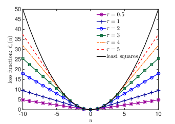
We refer to the Huber loss in Definition 1 above as the adaptive Huber loss to recognize the adaptivity of the robustification parameter $\tau$. For any $1\leq j\leq p$, with a robustification parameter $\tau_{j}>0$, we consider the following $M$-estimator of $\mu_{j}$:

$$\widehat{\mu}_{j}=\arg\min_{\theta\in\mathbb{R}}\sum_{i=1}^{n}\ell_{\tau_{j}}(X_{ij}-\theta),$$ (5)

where we suppress the dependence of $\widehat{\mu}_{j}$ on $\tau_{j}$ for simplicity. As shown in our theoretical results, the parameter $\tau$ plays an important role in controlling the bias-robustness tradeoff. To guarantee the asymptotic normality of $\widehat{\mu}_{j}$ uniformly over $j=1,\ldots p$, and to achieve optimal bias-robustness tradeoff, we choose $\tau=\tau(n,p)$ of the form $C\sqrt{{n}/{\log(np)}}$, where the constant $C>0$ can be selected via cross-validation. We refer to Section 4.1 for details. Specifically, we show that $\sqrt{n}\,(\widehat{\mu}_{j}-\bm{b}_{j}^{\mathrm{\scriptstyle T}}\bar{\bm{f}})$ is asymptotically normal with mean $\mu_{j}$ and variance $\sigma_{\varepsilon,jj}$ (with details given in Appendix B):

$$\sqrt{n}\,(\widehat{\mu}_{j}-\mu_{j}-\bm{b}^{\mathrm{\scriptstyle T}}_{j}\bar{\bm{f}}) =\mathcal{N}(0,\sigma_{\varepsilon,jj})+o_{\mathbb{P}}(1)~{}\mbox{ uniformly over }j=1,\ldots,p.$$ (6)

Here, $\widehat{\mu}_{j}$’s can be regarded as robust versions of the sample averages $\bar{X}_{j}=\mu_{j}+\bm{b}_{j}^{\mathrm{\scriptstyle T}}\bar{\bm{f}}+\bar{\varepsilon}_{j}$, where $\bar{X}_{j}=n^{-1}\sum_{i=1}^{n}X_{ij}$ and $\bar{\varepsilon}_{j}=n^{-1}\sum_{i=1}^{n}\varepsilon_{ij}$.

Given a prespecified level $\alpha\in(0,1)$, our testing procedure consists of three steps: (i) robust estimation of the loading vectors and factors; (ii) construction of factor-adjusted marginal test statistics and their $P$-values; and (iii) computing the critical value or threshold level with the estimated FDP controlled at $\alpha$. The detailed procedure is stated below.

FarmTest Procedure.

Input: Observed data $\bm{X}_{i}=(X_{i1},\ldots,X_{ip})^{\mathrm{\scriptstyle T}}\in\mathbb{R}^{p}$ for $i=1,\ldots,n$, a prespecified level $\alpha\in(0,1)$ and an integer $K\geq 1$.

Procedure:

Step 1: Construct a robust covariance matrix estimator $\widehat{\bm{\Sigma}}\in\mathbb{R}^{p\times p}$ based on observed data. Let $\widehat{\lambda}_{1}\geq\widehat{\lambda}_{2}\geq\cdots\geq\widehat{\lambda}_{K}$ be the top $K$ eigenvalues of $\widehat{\bm{\Sigma}}$, and $\widehat{\bm{v}}_{1},\widehat{\bm{v}}_{2},\ldots,\widehat{\bm{v}}_{K}$ be the corresponding eigenvectors. Define $\widehat{\mathbf{B}}=(\widetilde{\lambda}_{1}^{1/2}\widehat{\bm{v}}_{1},\ldots,\widetilde{\lambda}_{K}^{1/2}\widehat{\bm{v}}_{K})\in\mathbb{R}^{p\times K}$, where $\widetilde{\lambda}_{k}=\max(\widehat{\lambda}_{k},0)$. Let $\widehat{\bm{b}}_{1},\ldots,\widehat{\bm{b}}_{p}\in\mathbb{R}^{K}$ be the $p$ rows of $\widehat{\mathbf{B}}$, and define

$$\widehat{\bm{f}}\in\arg\min_{\bm{f}\in\mathbb{R}^{K}}\sum_{j=1}^{p}\ell_{\gamma}(\bar{X}_{j}-\widehat{\bm{b}}_{j}^{\mathrm{\scriptstyle T}}\bm{f}),$$ (7)

where $\gamma=\gamma(n,p)>0$ is a robustification parameter.

Step 2: Construct factor-adjusted test statistics

$${T}_{j}=\sqrt{\frac{n}{\widehat{\sigma}_{\varepsilon,jj}}}\,(\widehat{\mu}_{j}-\widehat{\bm{b}}_{j}^{\mathrm{\scriptstyle T}}\widehat{\bm{f}}\,),\ \ j=1,\ldots,p,$$ (8)

where $\widehat{\sigma}_{\varepsilon,jj}=\widehat{\theta}_{j}-\widehat{\mu}_{j}^{2}-\|\widehat{\bm{b}}_{j}\|_{2}^{2}$, $\widehat{\theta}_{j}=\arg\min_{\theta\geq\widehat{\mu}_{j}^{2}+\|\widehat{\bm{b}}_{j}\|_{2}^{2}}\sum_{i=1}^{n}\ell_{\tau_{jj}}(X_{ij}^{2}-\theta)$, $\tau_{jj}$’s are robustification parameters and $\widehat{\mu}_{j}$’s are defined in (5). Here, we use the fact that $\mathbb{E}(X_{j}^{2})=\mu_{j}^{2}+\|\bm{b}_{j}\|_{2}^{2}+\textnormal{var}(\varepsilon_{j})$, according to the identification condition.

Step 3: Calculate the critical value $z_{\alpha}$ as

$$z_{\alpha}=\inf\{z\geq 0:{{\rm FDP}}^{{\rm A}}(z)\leq\alpha\},$$ (9)

where ${{\rm FDP}}^{{\rm A}}(z)=2p\Phi(-z)/{R}(z)$ denotes the approximate FDP and $R(z)$ is as in (4). Finally, for $j=1,\ldots,p$, reject $H_{0j}$ whenever $|T_{j}|\geq z_{\alpha}$.

We expect that the factor-adjusted test statistic $T_{j}$ given in (8) is close in distribution to standard normal for all $j=1,\ldots,p$. Hence, according to the law of large numbers, the number of false discoveries $V(z)=\sum_{j\in\mathcal{H}_{0}}I(|T_{j}|\geq z)$ should be close to $2p_{0}\Phi(-z)$ for any $z\geq 0$. The number of null hypotheses $p_{0}$ is typically unknown. In the high dimensional and sparse regime, where both $p$ and $p_{0}$ are large and $p_{1}=p-p_{0}=o(p)$ is relatively small, ${\rm FDP}^{{\rm A}}$ in (9) serves as a slightly conservative surrogate for the asymptotic approximation $2p_{0}\Phi(-z)/{R}(z)$. If the proportion $\pi_{0}=p_{0}/p$ is bounded away from 1 as $p\to\infty$, ${\rm FDP}^{{\rm A}}$ tends to overestimate the true FDP. The estimation of $\pi_{0}$ has long been known as an interesting problem. See, for example, Storey (2002), Langaas and Lindqvist (2005), Meinshausen and Rice (2006), Jin and Cai (2007) and Jin (2008), among others. Therefore, a more adaptive method is to combine the above procedure with, for example Storey’s approach, to calibrate the rejection region for individual hypotheses. Let $\{P_{j}=2\Phi(-|T_{j}|)\}_{j=1}^{p}$ be the approximate $P$-values. For a predetermined $\eta\in[0,1)$, Storey (2002) suggested to estimate $\pi_{0}$ by

$$\widehat{\pi}_{0}(\eta)=\frac{1}{(1-\eta)p}\sum_{j=1}^{p}I(P_{j}>\eta).$$ (10)

The fundamental principle that underpins Storey’s procedure is that most of the large $P$-values come from the true null hypotheses and thus are uniformly distributed. For a sufficiently large $\eta$, about $(1-\eta)\pi_{0}$ of the $P$-values are expected to lie in $(\eta,1]$. Therefore, the proportion of $P$-values that exceed $\eta$ should be close to $(1-\eta)\pi_{0}$. A value of $\eta=1/2$ is used in the SAM software (Storey and Tibshirani, 2003); while it was shown in Blanchard and Roquain (2009) that the choice $\eta=\alpha$ may have better properties for dependent $P$-values.

Incorporating the above estimate of $\pi_{0}$, a modified estimate of ${\rm FDP}$ takes the form

$${\rm FDP}^{{\rm A}}(z;\eta)=2p\,\widehat{\pi}_{0}(\eta)\Phi(-z)/R(z),\,z\geq 0.$$

Finally, for any prespecified $\alpha\in(0,1)$, we reject $H_{0j}$ whenever $|T_{j}|\geq{z}_{\alpha,\eta}$, where

$${z}_{\alpha,\eta}=\inf\{z\geq 0:{\rm FDP}^{{\rm A}}(z;\eta)\leq\alpha\}.$$ (11)

By definition, it is easy to see that ${z}_{\alpha,0}$ coincides with $z_{\alpha}$ given in (9).

3 Theoretical properties

To fully understand the impact of factor-adjustment as well as robust estimation, we successively investigate the theoretical properties of the FarmTest through several steps, starting with an oracle procedure that provides key insights into the problem.

3.1 An oracle procedure

First we consider an oracle procedure that serves as a heuristic device. In this section, we assume the loading matrix $\mathbf{B}$ is known and the factors $\{\bm{f}_{i}\}_{i=1}^{n}$ are observable. In this case, it is natural to use the factor-adjusted data: $\bm{Y}_{i}=\bm{X}_{i}-\mathbf{B}\bm{f}_{i}=\bm{\mu}+\bm{\varepsilon}_{i}$, which has smaller componentwise variances (which are $\{\sigma_{\varepsilon,jj}\}_{j=1}^{p}$ and assumed known for the moment) than those of $\bm{X}_{i}$. Thus, instead of using $\sqrt{n}\,\widehat{\mu}_{j}$ given in (5), it is more efficient to construct robust mean estimates using factor-adjusted data. This is essentially the same as using the test statistic

$$T_{j}^{\circ}=\sqrt{\frac{n}{\sigma_{\varepsilon,jj}}}(\widehat{\mu}_{j}-\bm{b}_{j}^{\mathrm{\scriptstyle T}}\bar{\bm{f}}\,),$$ (12)

whose distribution is close to the standard normal distribution under the $j$-th null hypothesis. Recall that $p_{0}=|\mathcal{H}_{0}|$ is the number of true null hypotheses. Then, for any $z\geq 0$,

$$\frac{1}{p_{0}}V(z)=\frac{1}{p_{0}}\sum_{j\in\mathcal{H}_{0}}I(|T_{j}^{\circ}|\geq z).$$

Intuitively, the (conditional) law of large numbers suggests that $p_{0}^{-1}V(z)=2\Phi(-z)+o_{\mathbb{P}}(1)$. Hence, the FDP based on oracle test statistics admits an asymptotic expression

$${\rm AFDP}_{\rm orc}(z)=2p_{0}\Phi(-z)/R(z),\,z\geq 0,$$ (13)

where “AFDP” stands for the asymptotic FDP and a subscript “orc” is added to highlight its role as an oracle.

Remark 1.

For testing the individual hypothesis $H_{0j}$, Fan and Han (2017) considered the test statistic $\sqrt{n}\bar{X}_{j}$, where $\bar{X}_{j}=(1/n)\sum_{i=1}^{n}X_{ij}$. The empirical means, without factor adjustments, are inefficient as elucidated in Section 1. In addition, they are sensitive to the tails of error distributions (Catoni, 2012). In fact, with many collected variables, by chance only, some test statistics $\sqrt{n}\bar{X}_{j}$ can be so large in magnitude empirically that they may be mistakenly regarded as discoveries.

We will show that ${\rm AFDP}_{\rm orc}(z)$ provides a valid asymptotic approximation of the (unknown) true ${\rm FDP}$ using oracle statistics $\{T_{j}^{\circ}\}$ in high dimensions. The latter will be denoted as ${\rm FDP}_{{\rm orc}}(z)$. Let $\mathbf{R}_{\varepsilon}=(r_{\varepsilon,jk})_{1\leq j,k\leq p}$ be the correlation matrix of $\bm{\varepsilon}=(\varepsilon_{1},\ldots,\varepsilon_{p})^{\mathrm{\scriptstyle T}}$, that is, $\mathbf{R}_{\varepsilon}=\mathbf{D}_{\varepsilon}^{-1}\bm{\Sigma}_{\varepsilon}\mathbf{D}_{\varepsilon}^{-1}$ where $\mathbf{D}_{\varepsilon}^{2}={\rm diag}(\sigma_{\varepsilon,11},\ldots,\sigma_{\varepsilon,pp})$. Moreover, write

$$\omega_{n,p}=\sqrt{n/\log(np)}.$$ (14)

We impose the following moment and regularity assumptions.

Assumption 1.

(i) $p=p(n)\to\infty$ and $\log(p)=o(\sqrt{n})$ as $n\to\infty$; (ii) $\bm{X}\in\mathbb{R}^{p}$ follows the approximate factor model (1) with $\bm{f}$ and $\bm{\varepsilon}$ being independent; (iii) $\mathbb{E}(\bm{f})={\mathbf{0}}$, $\textnormal{cov}(\bm{f})=\mathbf{I}_{K}$ and $\|\bm{f}\|_{\psi_{2}}\leq A_{f}$ for some $A_{f}>0$, where $\|\cdot\|_{\psi_{2}}$ denotes the vector sub-Gaussian norm (Vershynin, 2018); (iv) There exist constants $C_{\varepsilon},c_{\varepsilon}>0$ such that $c_{\varepsilon}\leq\min_{1\leq j\leq p}\sigma_{\varepsilon,jj}^{1/2}\leq\max_{1\leq j\leq p}\upsilon_{j}\leq C_{\varepsilon}$, where $\upsilon_{j}:=(\mathbb{E}\varepsilon_{j}^{4})^{1/4}$; (v) There exist constants $\kappa_{0}\in(0,1)$ and $\kappa_{1}>0$ such that $\max_{1\leq j,k\leq p}|r_{\varepsilon,jk}|\leq\kappa_{0}$ and $p^{-2}\sum_{1\leq j,k\leq p}|r_{\varepsilon,jk}|=O(p^{-\kappa_{1}})$ as $p\to\infty$.

Part (iii) of Assumption 1 requires $\bm{f}\in\mathbb{R}^{K}$ to be a sub-Gaussian random vector. Typical examples include: (1) Gaussian and Bernoulli random vectors, (2) random vector that is uniformly distributed on the Euclidean sphere in $\mathbb{R}^{K}$ with center at the origin and radius $\sqrt{K}$, (3) random vector that is uniformly distributed on the Euclidean ball centered at the origin with radius $\sqrt{K}$, and (4) random vector that is uniformly distributed on the unit cube $[-1,1]^{K}$. In all these cases, the constant $A_{f}$ is a dimension-free constant. See Section 3.4 in Vershynin (2018) for detailed discussions of multivariate sub-Gaussian distributions. Part (v) is a technical condition on the covariance structure that allows $\varepsilon_{1},\ldots,\varepsilon_{p}$ to be weakly dependent. It relaxes the sparsity condition on the off-diagonal entries of $\bm{\Sigma}_{\varepsilon}$.

Theorem 1.

Suppose that Assumption 1 holds and $p_{0}\geq ap$ for some constant $a\in(0,1)$. Let $\tau_{j}=a_{j}\omega_{n,p}$ with $a_{j}\geq\sigma_{jj}^{1/2}$ for $j=1,\ldots,p$, where $\omega_{n,p}$ is given by (14). Then we have

$$p_{0}^{-1}V(z) =2\Phi(-z)+o_{\mathbb{P}}(1)$$ (15)

$$p^{-1}R(z) =\frac{1}{p}\sum_{j=1}^{p}\bigg{\{}\Phi\bigg{(}-z+\frac{\sqrt{n}\mu_{j}}{\sqrt{\sigma_{\varepsilon,jj}}}\bigg{)}+\Phi\bigg{(}-z-\frac{\sqrt{n}\mu_{j}}{\sqrt{\sigma_{\varepsilon,jj}}}\bigg{)}\bigg{\}}+o_{\mathbb{P}}(1)$$ (16)

uniformly over $z\geq 0$ as $n,p\to\infty$. Consequently, for any $z\geq 0$,

$$|{\rm FDP}_{{\rm orc}}(z)-{\rm AFDP}_{\rm orc}(z)|=o_{\mathbb{P}}(1)~{}\mbox{ as }n,p\to\infty.$$

3.2 Robust estimation of loading matrix

To realize the oracle procedure in practice, we need to estimate the loading matrix $\mathbf{B}$ and the covariance matrix $\bm{\Sigma}$, especially its diagonal entries. Before proceeding, we first investigate how these preliminary estimates affect FDP estimation. Assume at the moment that $\bar{\bm{f}}$ is given, let $\widetilde{\bm{b}}_{1},\ldots,\widetilde{\bm{b}}_{p}$ and $\widetilde{\sigma}_{11},\ldots,\widetilde{\sigma}_{pp}$ be generic estimates of $\bm{b}_{1},\ldots,\bm{b}_{p}$ and $\sigma_{11},\ldots,\sigma_{pp}$, respectively. In view of (2), $\sigma_{\varepsilon,jj}$ can be naturally estimated by $\widetilde{\sigma}_{jj}-\|\widetilde{\bm{b}}_{j}\|_{2}^{2}$. The corresponding FDP and its asymptotic approximation are given by

$$\widetilde{\rm FDP}(z)={\widetilde{V}(z)}/{\widetilde{R}(z)}~{}\mbox{ and }~{}\widetilde{\rm AFDP}(z)={2p_{0}\Phi(-z)}/{\widetilde{R}(z)},\ \ z\geq 0,$$

where $\widetilde{V}(z)=\sum_{j\in\mathcal{H}_{0}}I(|\widetilde{T}_{j}|\geq z)$, $\widetilde{R}(z)=\sum_{j=1}^{p}I(|\widetilde{T}_{j}|\geq z)$ and $\widetilde{T}_{j}=(n/\widetilde{\sigma}_{\varepsilon,jj})^{1/2}(\widehat{\mu}_{j}-\widetilde{\bm{b}}_{j}^{\mathrm{\scriptstyle T}}\bar{\bm{f}})$ for $j=1,\ldots,p$. The following proposition shows that to ensure consistent FDP approximation or furthermore estimation, it suffices to establish the uniform convergence results in (17) for the preliminary estimators of $\mathbf{B}$ and $\{\sigma_{jj}\}_{j=1}^{p}$. Later in Section 3.2.1 and 3.2.2, we propose two types of robust estimators satisfying (17) when $p=p(n)$ is allowed to grow exponentially fast with $n$.

Proposition 1.

Assume the conditions of Theorem 1 hold and that the preliminary estimates $\{\widetilde{\bm{b}}_{j},\widetilde{\sigma}_{jj}\}_{j=1}^{p}$ satisfy

$$\max_{1\leq j\leq p}\|\widetilde{\bm{b}}_{j}-\bm{b}_{j}\|_{2}=o_{\mathbb{P}}\{(\log n)^{-1/2}\},\quad\max_{1\leq j\leq p}|\widetilde{\sigma}_{jj}-\sigma_{jj}|=o_{\mathbb{P}}\{(\log n)^{-1/2}\}.$$ (17)

Then, for any $z\geq 0$, $|\widetilde{\rm FDP}(z)-\widetilde{\rm AFDP}(z)|=o_{\mathbb{P}}(1)$ as $n,p\to\infty$.

Next we focus on estimating $\mathbf{B}$ under identification condition (2). Write $\mathbf{B}=(\bar{\bm{b}}_{1},\ldots,\bar{\bm{b}}_{K})$ and assume without loss of generality that $\bar{\bm{b}}_{1},\ldots,\bar{\bm{b}}_{K}\in\mathbb{R}^{p}$ are ordered such that $\{\|\bar{\bm{b}}_{\ell}\|_{2}\}_{\ell=1}^{K}$ is in a non-increasing order. In this notation, we have $\bm{\Sigma}=\sum_{\ell=1}^{K}\bar{\bm{b}}_{\ell}\bar{\bm{b}}_{\ell}^{\mathrm{\scriptstyle T}}+\bm{\Sigma}_{\varepsilon}$, and $\bar{\bm{b}}_{\ell_{1}}^{\mathrm{\scriptstyle T}}\bar{\bm{b}}_{\ell_{2}}=0$ for $1\leq\ell_{1}\neq\ell_{2}\leq K$. Let $\lambda_{1},\ldots,\lambda_{p}$ be the eigenvalues of $\bm{\Sigma}$ in a descending order, with associated eigenvectors denoted by $\bm{v}_{1},\ldots,\bm{v}_{p}\in\mathbb{R}^{p}$. By Weyl’s theorem,

$$|\lambda_{j}-\|\bar{\bm{b}}_{j}\|_{2}^{2}|\leq\|\bm{\Sigma}_{\varepsilon}\|~{}\mbox{ for }1\leq j\leq K~{}\mbox{ and }~{}|\lambda_{j}|\leq\|\bm{\Sigma}_{\varepsilon}\|~{}\mbox{ for }j>K.$$

Moreover, under the pervasiveness condition (see Assumption 2 below), the eigenvectors $\bm{v}_{j}$ and $\bar{\bm{b}}_{j}/\|\bar{\bm{b}}_{j}\|_{2}$ of $\bm{\Sigma}$ and $\mathbf{B}\mathbf{B}^{\mathrm{\scriptstyle T}}$, respectively, are close to each other for $1\leq j\leq K$. The estimation of $\mathbf{B}$ thus depends heavily on estimating $\bm{\Sigma}$ along with its eigenstructure.

In Sections 3.2.1 and 3.2.2, we propose two different robust covariance matrix estimators that are also of independent interest. The construction of $\widehat{\mathbf{B}}$ then follows from Step 1 of the FarmTest procedure described in Section 2.2.

3.2.1 $U$-type covariance estimation

First, we propose a $U$-type covariance matrix estimator, which leads to estimates of the unobserved factors under condition (2). Let $\psi_{\tau}(\cdot)$ be the derivative of $\ell_{\tau}(\cdot)$ given by

$$\psi_{\tau}(u)=\min(|u|,\tau)\mathop{\mathrm{sign}}(u),\ \ u\in\mathbb{R}.$$

Given $n$ real-valued random variables $X_{1},\ldots,X_{n}$ from $X$ with mean $\mu$, a fast and robust estimator of $\mu$ is given by $\widehat{\mu}_{\tau}=(1/n)\sum_{i=1}^{n}\psi_{\tau}(X_{i})$. Minsker (2016) extended this univariate estimation scheme to matrix settings based on the following definition on matrix functionals.

Definition 2.

Given a real-valued function $f$ defined on $\mathbb{R}$ and a symmetric $\mathbf{A}\in\mathbb{R}^{d\times d}$ with eigenvalue decomposition $\mathbf{A}=\mathbf{U}\bm{\Lambda}\mathbf{U}^{\mathrm{\scriptstyle T}}$ such that $\bm{\Lambda}=\textnormal{diag}(\lambda_{1},\ldots,\lambda_{d})$, $f(\mathbf{A})$ is defined as $f(\mathbf{A})=\mathbf{U}f(\bm{\Lambda})\mathbf{U}^{\mathrm{\scriptstyle T}}$, where $f(\bm{\Lambda})=\textnormal{diag}(f(\lambda_{1}),\ldots,f(\lambda_{d}))$.

Suppose we observe $n$ random samples $\bm{X}_{1},\ldots,\bm{X}_{n}$ from $\bm{X}$ with mean $\bm{\mu}$ and covariance matrix $\bm{\Sigma}=\mathbb{E}\{(\bm{X}-\bm{\mu})(\bm{X}-\bm{\mu})^{\mathrm{\scriptstyle T}}\}$. If $\bm{\mu}$ were known, a robust estimator of $\bm{\Sigma}$ can be simply constructed by $(1/n)\sum_{i=1}^{n}\psi_{\tau}\{(\bm{X}_{i}-\bm{\mu})(\bm{X}_{i}-\bm{\mu})^{\mathrm{\scriptstyle T}}\}$. In practice, the assumption of a known $\bm{\mu}$ is often unrealistic. Instead, we suggest to estimate $\bm{\Sigma}$ using the following $U$-statistic based estimator:

$$\widehat{\bm{\Sigma}}_{U}(\tau)=\frac{1}{\binom{n}{2}}\sum_{1\leq i<j\leq n}\psi_{\tau}\bigg{\{}\frac{1}{2}(\bm{X}_{i}-\bm{X}_{j})(\bm{X}_{i}-\bm{X}_{j})^{\mathrm{\scriptstyle T}}\bigg{\}}.$$

Observe that $(\bm{X}_{i}-\bm{X}_{j})(\bm{X}_{i}-\bm{X}_{j})^{\mathrm{\scriptstyle T}}$ is a rank one matrix with eigenvalue $\|\bm{X}_{i}-\bm{X}_{j}\|_{2}^{2}$ and eigenvector $(\bm{X}_{i}-\bm{X}_{j})/\|\bm{X}_{i}-\bm{X}_{j}\|_{2}$. Therefore, by Definition 2, $\widehat{\bm{\Sigma}}_{U}(\tau)$ can be equivalently written as

$$\frac{1}{\binom{n}{2}}\sum_{1\leq i<j\leq n}\psi_{\tau}\bigg{(}\frac{1}{2}\|\bm{X}_{i}-\bm{X}_{j}\|_{2}^{2}\bigg{)}\frac{(\bm{X}_{i}-\bm{X}_{j})(\bm{X}_{i}-\bm{X}_{j})^{\mathrm{\scriptstyle T}}}{\|\bm{X}_{i}-\bm{X}_{j}\|_{2}^{2}}.$$ (18)

This alternative expression makes it much easier to compute. The following theorem provides an exponential-type deviation inequality for $\widehat{\bm{\Sigma}}_{U}(\tau)$, representing a useful complement to the results in Minsker (2016). See, for example, Remark 8 therein.

Theorem 2.

Let

$$v^{2}=\frac{1}{2}\Big{\|}\mathbb{E}\{(\bm{X}-\bm{\mu})(\bm{X}-\bm{\mu})^{\mathrm{\scriptstyle T}}\}^{2}+\mathop{\mathrm{tr}}(\bm{\Sigma})\bm{\Sigma}+2\bm{\Sigma}^{2}\Big{\|}.$$ (19)

For any $t>0$, the estimator $\widehat{\bm{\Sigma}}_{U}=\widehat{\bm{\Sigma}}_{U}(\tau)$ with $\tau\geq(v/2)(n/t)^{1/2}$ satisfies

$$\mathbb{P}\{\|\widehat{\bm{\Sigma}}_{U}-\bm{\Sigma}\|\geq 4v(t/n)^{1/2}\}\leq 2p\exp(-t).$$

Given $\widehat{\bm{\Sigma}}_{U}$, we can construct an estimator of $\mathbf{B}$ following Step 1 of the FarmTest procedure. Recall that $\widehat{\bm{b}}_{1},\ldots,\widehat{\bm{b}}_{p}$ are the $p$ rows of $\widehat{\mathbf{B}}$. To investigate the consistency of $\widehat{\bm{b}}_{j}$’s, let $\overline{\lambda}_{1},\ldots,\overline{\lambda}_{K}$ be the top $K$ (nonzero) eigenvalues of $\mathbf{B}\mathbf{B}^{\mathrm{\scriptstyle T}}$ in a descending order and $\overline{\bm{v}}_{1},\ldots,\overline{\bm{v}}_{K}$ be the corresponding eigenvectors. Under identification condition (2), we have $\overline{\lambda}_{\ell}=\|\overline{\bm{b}}_{\ell}\|_{2}^{2}$ and $\overline{\bm{v}}_{\ell}=\overline{\bm{b}}_{\ell}/\|\overline{\bm{b}}_{\ell}\|_{2}$ for $\ell=1,\ldots,K$.

Assumption 2 (Pervasiveness).

There exist positive constants $c_{1}$, $c_{2}$ and $c_{3}$ such that $c_{1}p\leq\overline{\lambda}_{\ell}-\overline{\lambda}_{\ell+1}\leq c_{2}p$ for $\ell=1,\ldots,K$ with $\overline{\lambda}_{K+1}:=0$, and $\|\bm{\Sigma}_{\varepsilon}\|\leq c_{3}<\overline{\lambda}_{K}$.

Remark 2.

The pervasiveness condition is required for high dimensional spiked covariance model with the first several eigenvalues well separated and significantly larger than the rest. In particular, Assumption 2 requires the top $K$ eigenvalues grow linearly with the dimension $p$. The corresponding eigenvectors can therefore be consistently estimated as long as sample size diverges (Fan et al., 2013). This condition is widely assumed in the literature (Stock and Watson, 2002; Bai and Ng, 2002). The following proposition provides convergence rates of the robust estimators $\{\widehat{\lambda}_{\ell},\widehat{\bm{v}}_{\ell}\}_{\ell=1}^{K}$ under Assumption 2. The proof, which is given in in Appendix D, is based on Weyl’s inequality and a useful variant of the Davis-Kahan theorem (Yu et al., 2015). We notice that some preceding works (Onatski, 2012; Shen et al., 2016; Wang and Fan, 2017) have provided similar results under a weaker pervasiveness assumption which allows $p/n\rightarrow\infty$ in any manner and the spiked eigenvalues $\{\overline{\lambda}_{\ell}\}_{\ell=1}^{K}$ are allowed to grow slower than $p$ so long as $c_{\ell}=p/(n\overline{\lambda}_{\ell})$ is bounded.

Proposition 2.

Under Assumption 2, we have

$$\max_{1\leq\ell\leq K}|\widehat{\lambda}_{\ell}-\overline{\lambda}_{\ell}|\leq\|\widehat{\bm{\Sigma}}_{U}-\bm{\Sigma}\|+\|\bm{\Sigma}_{\varepsilon}\|~{}~{}\textnormal{and}$$ (20)

$$\max_{1\leq\ell\leq K}\|\widehat{\bm{v}}_{\ell}-\overline{\bm{v}}_{\ell}\|_{2}\leq Cp^{-1}(\|\widehat{\bm{\Sigma}}_{U}-\bm{\Sigma}\|+\|\bm{\Sigma}_{\varepsilon}\|),$$ (21)

where $C>0$ is a constant independent of $(n,p)$.

We now show the properties of estimated loading vectors and estimated residual variances $\{\widehat{\sigma}_{\varepsilon,jj}\}_{j=1}^{p}$ that are defined below (8).

Theorem 3.

Suppose Assumption 1(iv) and Assumption 2 hold. Let $\tau=v_{0}\omega_{n,p}$ with $v_{0}\geq v/2$ for $v$ given in (19). Then, with probability at least $1-2n^{-1}$,

$$\max_{1\leq j\leq p}\|\widehat{\bm{b}}_{j}-{\bm{b}}_{j}\|_{2}\leq C_{1}\{v\sqrt{\log(np)}\,(np)^{-1/2}+p^{-1/2}\}$$ (22)

as long as $n\geq v^{2}p^{-1}\log(np)$. In addition, if $n\geq C_{2}\log(np)$, $\tau_{j}=a_{j}\omega_{n,p},\tau_{jj}=a_{jj}\omega_{n,p}$ with $a_{j}\geq\sigma_{jj}^{1/2},a_{jj}\geq\textnormal{var}(X_{j}^{2})^{1/2}$, we have

$$\max_{1\leq j\leq p}|\widehat{\sigma}_{\varepsilon,jj}-\sigma_{\varepsilon,jj}|\leq C_{3}(vp^{-1/2}w_{n,p}^{-1}+p^{-1/2})$$ (23)

with probability greater than $1-C_{4}n^{-1}$. Here, $C_{1}$–$C_{4}$ are positive constants that are independent of $(n,p)$.

Remark 3.

According to Theorem 3, the robustification parameters can be set as $\tau_{j}=a_{j}\omega_{n,p}$ and $\tau_{jj}=a_{jj}\omega_{n,p}$, where $w_{n,p}$ is given in (14). In practice, the constants $a_{j}$ and $a_{jj}$ can be chosen by cross-validation.

3.2.2 Adaptive Huber covariance estimation

In this section, we adopt an estimator that was first considered in Fan et al. (2017). For every $1\leq j\neq k\leq p$, we define the robust estimate $\widehat{\sigma}_{jk}$ of $\sigma_{jk}=\mathbb{E}(X_{j}X_{k})-\mu_{j}\mu_{k}$ to be

$$\widehat{\sigma}_{jk}=\widehat{\theta}_{jk}-\widehat{\mu}_{j}\widehat{\mu}_{k}~{}\mbox{ with }~{}\widehat{\theta}_{jk}=\arg\min_{\theta\in\mathbb{R}}\sum_{i=1}^{n}\ell_{\tau_{jk}}(X_{ij}X_{ik}-\theta),$$ (24)

where $\tau_{jk}>0$ is a robustification parameter and $\widehat{\mu}_{j}$ is defined in (5). This yields the adaptive Huber covariance estimator $\widehat{\bm{\Sigma}}_{{\rm H}}=(\widehat{\sigma}_{jk})_{1\leq j,k\leq p}$. The dependence of $\widehat{\bm{\Sigma}}_{{\rm H}}$ on $\{\tau_{jk}:1\leq j\leq k\leq p\}$ and $\{\tau_{j}\}_{j=1}^{p}$ is assumed without displaying.

Theorem 4.

Suppose Assumption 1(iv) and Assumption 2 hold. Let $\tau_{j}=a_{j}\omega_{n,p},\tau_{jk}=a_{jk}\omega_{n,p^{2}}$ with $a_{j}\geq\sigma_{jj}^{1/2},a_{jk}\geq\textnormal{var}(X_{j}^{2})^{1/2}$ for $1\leq j,k\leq p$. Then, there exist positive constants $C_{1}$–$C_{3}$ independent of $(n,p)$ such that as long as $n\geq C_{1}\log(np)$,

$$\max_{1\leq j\leq p}\|\widehat{\bm{b}}_{j}-{\bm{b}}_{j}\|_{2}\leq C_{2}(\omega_{n,p}^{-1}+p^{-1/2})$$

$$\mbox{ and }~{}\max_{1\leq j\leq p}|\widehat{\sigma}_{\varepsilon,jj}-\sigma_{\varepsilon,jj}|\leq C_{3}(\omega_{n,p}^{-1}+p^{-1/2})$$

with probability greater than $1-4n^{-1}$, where $w_{n,p}$ is given in (14).

3.3 Estimating realized factors

To make the oracle statistics $T_{j}^{\circ}$’s given in (12) usable, it remains to estimate $\bar{\bm{f}}$. Since the loadings can be estimated in two different ways, let us first assume $\mathbf{B}$ is given and treat it as an input variable.

Averaging the approximate factor model (1), we have $\bar{\bm{X}}=\bm{\mu}+\mathbf{B}\bar{\bm{f}}+\bar{\bm{\varepsilon}}$, where $\bar{\bm{X}}=(\bar{X}_{1},\ldots,\bar{X}_{p})^{\mathrm{\scriptstyle T}}=(1/n)\sum_{i=1}^{n}\bm{X}_{i}$ and $\bar{\bm{\varepsilon}}:=(\bar{\varepsilon}_{1},\ldots,\bar{\varepsilon}_{p})^{\mathrm{\scriptstyle T}}=(1/n)\sum_{i=1}^{n}\bm{\varepsilon}_{i}$. This leads to

$$\bar{X}_{j}=\bm{b}_{j}^{\mathrm{\scriptstyle T}}\bar{\bm{f}}+\mu_{j}+\bar{\varepsilon}_{j},\ \ j=1,\ldots,p.$$ (25)

Among all $\{\mu_{j}+\bar{\varepsilon}_{j}\}_{j=1}^{p}$, we may regard $\mu_{j}+\bar{\varepsilon}_{j}$ with $\mu_{j}\neq 0$ as outliers. Therefore, to achieve robustness, we estimate $\bar{\bm{f}}$ by solving the following optimization problem:

$$\widehat{\bm{f}}(\mathbf{B})\in\arg\min_{\bm{f}\in\mathbb{R}^{K}}\sum_{j=1}^{p}\ell_{\gamma}(\bar{X}_{j}-\bm{b}_{j}^{\mathrm{\scriptstyle T}}\bm{f}),$$ (26)

where $\gamma=\gamma(n,p)>0$ is a robustification parameter. Next, we define robust variance estimators $\widehat{\sigma}_{\varepsilon,jj}$’s by

$$\widehat{\sigma}_{\varepsilon,jj}(\mathbf{B})=\widehat{\theta}_{j}-\widehat{\mu}_{j}^{2}-\|\bm{b}_{j}\|_{2}^{2}~{}\mbox{ with }~{}\widehat{\theta}_{j}=\arg\min_{\theta\,\geq\,\widehat{\mu}_{j}^{2}+\|\bm{b}_{j}\|_{2}^{2}}\sum_{i=1}^{n}\ell_{\tau_{jj}}(X_{ij}^{2}-\theta),$$

where $\tau_{jj}$’s are robustification parameters and $\widehat{\mu}_{j}$’s are as in (5). Plugging $\{\widehat{\sigma}_{\varepsilon,jj}\}_{j=1}^{p}$ and $\widehat{\bm{f}}$ into (12), we obtain the following factor-adjusted test statistics

$${T}_{j}(\mathbf{B})=\bigg{\{}\frac{n}{\widehat{\sigma}_{\varepsilon,jj}(\mathbf{B})}\bigg{\}}^{1/2}\{\widehat{\mu}_{j}-{\bm{b}}_{j}^{\mathrm{\scriptstyle T}}\widehat{\bm{f}}(\mathbf{B})\},\ \ j=1,\ldots,p.$$ (27)

For a given threshold $z\geq 0$, the corresponding FDP is defined as

$${{\rm FDP}}(z;\mathbf{B})={V}(z;\mathbf{B})/{R}(z;\mathbf{B}),$$

where ${V}(z;\mathbf{B})=\sum_{j\in\mathcal{H}_{0}}I\{|{T}_{j}(\mathbf{B})|\geq z\}$ and ${R}(z;\mathbf{B})=\sum_{1\leq j\leq p}I\{|{T}_{j}(\mathbf{B})|\geq z\}.$ Similarly to (13), we approximate ${{\rm FDP}}(z;\mathbf{B})$ by

$${\rm AFDP}(z;\mathbf{B})=2p_{0}\Phi(-z)/R(z;\mathbf{B}).$$

For any $z\geq 0$, the approximate FDP ${\rm AFDP}(z;\mathbf{B})$ is computable except $p_{0}$, which can be either estimated (Storey, 2002) or upper bounded by $p$. Albeit being slightly conservative, the latter proposal is accurate enough in the sparse setting.

Regarding the accuracy of ${\rm AFDP}(z;\mathbf{B})$ as an asymptotic approximation of ${{\rm FDP}}(z;\mathbf{B})$, we need to account for the statistical errors of $\{\widehat{\sigma}_{\varepsilon,jj}(\mathbf{B})\}_{j=1}^{p}$ and $\widehat{\bm{f}}(\mathbf{B})$. To this end, we make the following structural assumptions on $\bm{\mu}$ and $\mathbf{B}$.

Assumption 3.

The idiosyncratic errors $\varepsilon_{1},\ldots,\varepsilon_{p}$ are mutually independent, and there exist constants $c_{l},c_{u}>0$ such that $\lambda_{\min}(p^{-1}\mathbf{B}^{\mathrm{\scriptstyle T}}\mathbf{B})\geq c_{l}$ and $\|\mathbf{B}\|_{\max}\leq c_{u}$.

Assumption 4 (Sparsity).

There exist constants $C_{\mu}>0$ and $c_{\mu}\in(0,1/2)$ such that $\|\bm{\mu}\|_{\infty}=\max_{1\leq j\leq p}|\mu_{j}|\leq C_{\mu}$ and $\|\bm{\mu}\|_{0}=\sum_{j=1}^{p}I(\mu_{j}\neq 0)\leq p^{1/2-c_{\mu}}$. Moreover, $(n,p)$ satisfies that $n\log(n)=o(p)$ as $n,p\to\infty$.

The following proposition, which is of independent interest, reveals an exponential-type deviation inequality for $\widehat{\bm{f}}(\mathbf{B})$ with a properly chosen $\gamma>0$.

Proposition 3.

Suppose that Assumption 3 holds. For any $t>0$, the estimator $\widehat{\bm{f}}(\mathbf{B})$ given in (26) with $\gamma=\gamma_{0}(p/t)^{1/2}$ for $\gamma_{0}\geq\overline{\sigma}_{\varepsilon}:=(p^{-1}\sum_{j=1}^{p}\sigma_{\varepsilon,jj})^{1/2}$ satisfies that with probability greater than $1-(2eK+1)e^{-t}$,

$$\|\widehat{\bm{f}}(\mathbf{B})-\bar{\bm{f}}\|_{2}\leq C_{1}\gamma_{0}(Kt)^{1/2}p^{-1/2}$$ (28)

as long as $p\geq\max\{\|\bm{\mu}\|_{2}^{2}/\overline{\sigma}_{\varepsilon}^{2},(\|\bm{\mu}\|_{1}/\overline{\sigma}_{\varepsilon})^{2}t,C_{2}K^{2}t\}$, where $C_{1},C_{2}>0$ are constants depending only on $c_{l},c_{u}$ in Assumption 3.

The convergence in probability of ${{\rm FDP}}(z;\mathbf{B})$ to ${\rm AFDP}(z;\mathbf{B})$ for any $z\geq 0$ is investigated in the following theorem.

Theorem 5.

Suppose that Assumptions 1 (i)–(iv), Assumptions 3 and 4 hold. Let $\tau_{j}=a_{j}\omega_{n,p}$, $\tau_{jj}=a_{jj}\omega_{n,p}$ with $a_{j}\geq\sigma_{jj}^{1/2}$, $a_{jj}\geq\textnormal{var}(X_{j}^{2})^{1/2}$ for $j=1,\ldots,p$, and $\gamma=\gamma_{0}\{p/\log(n)\}^{1/2}$ with $\gamma_{0}\geq\overline{\sigma}_{\varepsilon}$. Then, for any $z\geq 0$, $|{{\rm FDP}}(z;\mathbf{B})-{\rm AFDP}(z;\mathbf{B})|=o_{\mathbb{P}}(1)$ as $n,p\to\infty$.

4 Simulation studies

4.1 Selecting robustification parameters

The robustification parameter involved in the Huber loss plays an important role in the proposed procedures both theoretically and empirically. In this section, we describe the use of cross-validation to calibrate robustification parameter in practice. To highlight the main idea, we restrict our attention to the mean estimation problem.

Suppose we observe $n$ samples $X_{1},\ldots,X_{n}$ from $X$ with mean $\mu$. For any given $\tau>0$, the Huber estimator is defined as $\widehat{\mu}_{\tau}=\arg\min_{\theta\in\mathbb{R}}\sum_{i=1}^{n}\ell_{\tau}(X_{i}-\theta)$, or equivalently, the unique solution of the equation $\sum_{i=1}^{n}\psi_{\tau}(X_{i}-\theta)=0$. Our theoretical analysis suggests that the theoretically optimal $\tau$ is of the form $C_{\sigma}\omega_{n}$, where $\omega_{n}$ is a specified function of $n$ and $C_{\sigma}>0$ is a constant that scales with $\sigma$, the standard deviation of $X$. This allows us to narrow down the search range by selecting $C_{\sigma}$ instead via the $K$-fold ($K=5$ or 10) cross-validation as follows. First, we randomly divide the sample into $K$ subsets, ${\cal I}_{1},\ldots,\mathcal{I}_{K}$, with roughly equal sizes. The cross-validation criterion for a given $C>0$ can be defined as

$${\rm CV}(C)=\frac{1}{n}\sum\limits_{k=1}^{K}\sum\limits_{i\in{\cal I}_{k}}\{X_{i}-\widehat{\mu}^{(-k)}_{\tau_{C}}\}^{2},$$ (29)

where $\widehat{\mu}^{(-k)}_{\tau_{C}}$ is the Huber estimator using data not in the $k$-th fold, namely

$$\widehat{\mu}^{(-k)}_{\tau_{C}}=\arg\min_{\theta\in\mathbb{R}}\sum_{\ell=1,\ell\neq k}^{K}\sum_{i\in{\cal I}_{\ell}}\ell_{\tau_{C}}(X_{i}-\theta),$$

and $\tau_{C}=C\omega_{n}$. In practice, let $\cal C$ be a set of grid points for $C$. We choose $C_{\sigma}$ and therefore $\tau$ by $\widehat{C}_{\sigma}=\arg\min_{C\in{\cal C}}{\rm CV}(C)$ and $\widehat{\tau}=\widehat{C}_{\sigma}\omega_{n}$.

The robustification parameters involved in the FarmTest procedure can be selected in a similar fashion by modifying the loss function and the cross-validation criterion (29) accordingly. The theoretical order $\omega_{n}$ can be chosen as the rate that guarantees optimal bias-robustness tradeoff. Based on the theoretical results in Section 3, we summarize the optimal rates for various robustification parameters in Table 1. Robust estimation of $\mu_{j}$’s and the adaptive Huber covariance estimator involve multiple robustification parameters. If $X_{1},\ldots,X_{p}$ are homoscedastic, it is reasonable to assume $\tau_{j}=\tau_{\mu}$ in (5) for all $j=1,\ldots,p$. Then we can choose $\tau_{\mu}$ by applying the cross-validation over a small subset of the covariates $X_{1},\ldots,X_{p}$. Similarly, we can set $\tau_{jk}=\tau_{\Sigma}$ in (24) for all $j,k$ and calibrate $\tau_{\Sigma}$ by applying the cross-validation over a subset of the entries.

Table 1: Optimal rates for robustification parameters

Estimator	Parameter	Optimal Rate
Robust estimator of $\mu_{j}$	$\tau_{j}$ in (5)	$\sqrt{n/\log(np)}$
$U$-type covariance estimator	$\tau$ in (18)	$p\sqrt{n/\log(p)}$
Adaptive Huber covariance estimator	$\tau_{jk}$ in (24)	$\sqrt{n/\log(np^{2})}$
Robust estimator of $\bar{\bm{f}}$	$\gamma$ in (26)	$\sqrt{p/\log(n)}$

4.2 Settings

In the simulation studies, we take $(p_{1},p)=(25,500)$ so that $\pi_{1}=p_{1}/p=0.05$, $n\in\{100,150,200\}$ and use $t=0.01$ as the threshold value for $P$-values. Moreover, we set the mean vector $\bm{\mu}=(\mu_{1},\ldots,\mu_{p})^{\mathrm{\scriptstyle T}}$ to be $\mu_{j}=0.5$ for $1\leq j\leq 25$ and $\mu_{j}=0$ otherwise. We repeat 1000 replications in each of the scenarios below. The robustifications parameters are selected by five-fold cross-validation under the guidance of their theoretically optimal orders. The data-generating processes are as follows.

Model 1: Normal factor model. Consider a three-factor model $\bm{X}_{i}=\bm{\mu}+\mathbf{B}\bm{f}_{i}+\bm{\varepsilon}_{i}$, $i=1,\ldots,n$, where $\bm{f}_{i}\sim\mathcal{N}(\mathbf{0},\mathbf{I}_{3})$, $\mathbf{B}=(b_{j\ell})_{1\leq j\leq p,1\leq\ell\leq 3}$ has IID entries $b_{j\ell}$’s generated from the uniform distribution $\mathcal{U}(-2,2)$.

Model 2: Synthetic factor model. Consider a similar three-factor model as in Model 1, except that $\bm{f}_{i}$’s and $\bm{b}_{j}$’s are generated independently from $\mathcal{N}(\mathbf{0},\bm{\Sigma}_{f})$ and $\mathcal{N}(\bm{\mu}_{B},\bm{\Sigma}_{B})$, respectively, where $\bm{\Sigma}_{f}$, $\bm{\mu}_{B}$ and $\bm{\Sigma}_{B}$ are calibrated from the daily returns of S&P 500’s top 100 constituents (ranked by the market cap) between July 1st, 2008 and June 29th, 2012.

Model 3: Serial dependent factor model. Consider a similar three-factor model as in Model 1, except that $\bm{f}_{i}$’s are generated from a stationary VAR$(1)$ model $\bm{f}_{i}={\bf\Pi}\bm{f}_{i-1}+{\bm{\xi}}_{i}$ for $i=1,\ldots,n$, with $\bm{f}_{0}={\bf 0}$ and $\bm{\xi}_{i}$’s IID drawn from $\mathcal{N}({\bf 0},\mathbf{I}_{3})$. The $(j,k)$-th entry of ${\bf\Pi}$ is set to be 0.5 when $j=k$ and $0.4^{|j-k|}$ otherwise.

The idiosyncratic errors in these three models are generated from one of the following four distributions. Let $\bm{\Sigma}_{\bm{\varepsilon}}$ be a sparse matrix whose diagonal entries are 3 and off-diagonal entries are drawn from IID $0.3\times{\rm Bernoulli}(0.05)$;

• Multivariate normal distribution $\mathcal{N}(\mathbf{0},\bm{\Sigma}_{\bm{\varepsilon}})$;

• Multivariate $t$-distribution $t_{3}(\mathbf{0},\bm{\Sigma}_{\bm{\varepsilon}})$ with 3 degrees of freedom;

• IID Gamma distribution with shape parameter 3 and scale parameter 1;

• IID re-scaled log-normal distribution $a\{\exp(1+1.2Z)-b\}$, where $Z\sim\mathcal{N}(0,1)$ and $a,b>0$ are chosen such that it has mean zero and variance $3$.

4.3 FDP estimation

In our robust testing procedure, the covariance matrix is either estimated by the entry-wise adaptive Huber method or by the $U$-type robust covariance estimator. The corresponding tests are labeled as FARM-H and FARM-$U$, respectively.

In this section, we compare FARM-H and FARM-$U$ with three existing non-robust tests. The first one is a factor-adjusted procedure using the sample mean and sample covariance matrix, denoted by FAM. The second one is the PFA method, short for principal factor approximation, proposed by Fan and Han (2017). In contrast to FAM, PFA directly uses the unadjusted test statistics and only accounts for the effect of latent factors in FDP estimation. The third non-robust procedure is the Naive method, which completely ignores the factor dependence.

We first examine the accuracy of FDP estimation, which is assessed by the median of the relative absolute error (RAE) between the estimated FDP and ${\rm FDP}_{{\rm orc}}(t):=\frac{\sum_{j\in\mathcal{H}_{0}}I(P_{j}\leq t)}{\max\{1,\sum_{j=1}^{p}I(P_{j}\leq t)\}}$, where $P_{j}=2\Phi(-|T_{j}^{{\rm o}}|)$ and $T_{j}^{{\rm o}}$ are the oracle test statistics given in (12). For a given threshold value $t$, RAE for $k$th simulation is defined as

$$\mathrm{RAE}(k)=|\widehat{{\rm FDP}}(t,k)-{\rm FDP}_{{\rm orc}}(t,k)|/{\rm FDP}_{{\rm orc}}(t,k),\quad k=1,\ldots,1000,$$

where $\widehat{{\rm FDP}}(t,k)$ is the estimated FDP in the $k$th simulation using one of the five competing methods and ${\rm FDP}_{{\rm orc}}(t,k)$ is the oracle FDP in the $k$th experiment. The median of RAEs are presented in Table 2. We see that, although the PFA and FAM methods achieve the smallest estimation errors in the normal case, FARM-H and FARM-$U$ perform comparably well. In other words, a high level of efficiency is achieved if the underlying distribution is normal. The Naive method performs worst as it ignores the impact of the latent factors. In heavy-tailed cases, both FARM-H and FARM-$U$ outperform the non-robust competitors by a wide margin, still with the Naive method being the least favorable. In summary, the proposed methods achieve high degree of robustness against heavy-tailed errors, while losing little or no efficiency under normality.

Table 2: Median relative absolute error between estimated and oracle FDP

			$p=500$
	$\bm{\varepsilon}_{i}$	$n$	FARM-H	FARM-$U$	FAM	PFA	Naive
Model 1	Normal	100	0.8042	0.8063	0.7716	0.7487	1.789
		150	0.7902	0.7925	0.7467	0.7790	1.599
		200	0.7665	0.7743	0.7437	0.7363	1.538
	$t_{3}$	100	0.7047	0.7539	1.3894	1.4676	2.061
		150	0.6817	0.6002	1.1542	1.2490	1.801
		200	0.6780	0.5244	0.9954	1.1306	1.579
	Gamma	100	0.7034	0.7419	1.4986	1.7028	3.299
		150	0.6844	0.6869	1.4396	1.5263	2.844
		200	0.6393	0.6446	1.3911	1.4563	2.041
	LN	100	0.6943	0.7104	1.5629	1.7255	3.292
		150	0.6487	0.6712	1.6128	1.7742	3.092
		200	0.6137	0.6469	1.4476	1.4927	2.510
Model 2	Normal	100	0.6804	0.7079	0.6195	0.6318	1.676
		150	0.6928	0.6873	0.6302	0.6136	1.573
		200	0.6847	0.6798	0.6037	0.6225	1.558
	$t_{3}$	100	0.6438	0.6641	1.3939	1.4837	2.206
		150	0.6258	0.6466	1.2324	1.2902	1.839
		200	0.6002	0.6245	1.0368	1.0811	1.481
	Gamma	100	0.6404	0.6493	1.6743	1.7517	3.129
		150	0.5979	0.5991	1.3618	1.4405	2.657
		200	0.5688	0.5746	1.0803	1.1595	2.035
	LN	100	0.7369	0.7793	2.0022	2.0427	3.664
		150	0.6021	0.6122	1.7935	1.8796	3.056
		200	0.5557	0.5588	1.6304	1.8059	2.504
Model 3	Normal	100	0.7937	0.8038	0.7338	0.7651	1.991
		150	0.7617	0.7750	0.7415	0.7565	1.888
		200	0.7544	0.7581	0.7428	0.7440	1.858
	$t_{3}$	100	0.7589	0.7397	1.4302	1.6053	2.105
		150	0.6981	0.7010	1.2980	1.3397	1.956
		200	0.6596	0.6846	1.1812	1.1701	1.847
	Gamma	100	0.7134	0.7391	1.7585	1.9981	3.945
		150	0.6609	0.6744	1.5449	1.7437	3.039
		200	0.6613	0.6625	1.4650	1.4869	2.295
	LN	100	0.7505	0.7330	1.8019	1.9121	3.830
		150	0.6658	0.7015	1.7063	1.7669	3.278
		200	0.6297	0.6343	1.5944	1.6304	2.937

4.4 Power performance

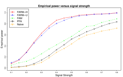
In this section, we compare the powers of the five methods under consideration. The empirical power is defined as the average ratio between the number of correct rejections and $p_{1}$. The results are displayed in Table 3. In the normal case, FAM has a higher power than PFA. This is because FAM adjusts the effect of latent factors for each individual hypothesis so that the signal-to-noise ratio is higher. Again, both FARM-H and FARM-$U$ tests only pay a negligible price in power under normality. In heavy-tailed cases, however, these two robust methods achieve much higher empirical powers than their non-robust counterparts. Moreover, to illustrate the relationship between the empirical power and signal strength, Figure 3 displays the empirical power versus signal strength ranging from 0.1 to 0.8 for Model 1 with $(n,p)=(200,500)$ and $t_{3}$-distributed errors.

Table 3: Empirical powers

			$p=500$
	$\bm{\varepsilon}_{i}$	$n$	FARM-H	FARM-$U$	FAM	PFA	Naive
Model 1	Normal	100	0.853	0.849	0.872	0.863	0.585
		150	0.877	0.870	0.890	0.882	0.624
		200	0.909	0.907	0.924	0.915	0.671
	$t_{3}$	100	0.816	0.815	0.630	0.610	0.442
		150	0.828	0.826	0.668	0.657	0.464
		200	0.894	0.870	0.702	0.691	0.502
	Gamma	100	0.816	0.813	0.658	0.639	0.281
		150	0.830	0.825	0.684	0.663	0.391
		200	0.889	0.873	0.712	0.707	0.433
	LN	100	0.798	0.786	0.566	0.534	0.242
		150	0.817	0.805	0.587	0.673	0.292
		200	0.844	0.835	0.613	0.605	0.369
Model 2	Normal	100	0.801	0.799	0.864	0.855	0.584
		150	0.856	0.846	0.880	0.870	0.621
		200	0.904	0.900	0.911	0.904	0.659
	$t_{3}$	100	0.810	0.802	0.612	0.601	0.402
		150	0.825	0.814	0.638	0.632	0.457
		200	0.873	0.859	0.695	0.683	0.484
	Gamma	100	0.804	0.798	0.527	0.509	0.216
		150	0.821	0.819	0.594	0.557	0.289
		200	0.885	0.875	0.638	0.606	0.379
	LN	100	0.763	0.757	0.463	0.434	0.206
		150	0.799	0.795	0.495	0.479	0.228
		200	0.826	0.819	0.529	0.511	0.312
Model 3	Normal	100	0.837	0.832	0.848	0.833	0.535
		150	0.856	0.848	0.864	0.857	0.594
		200	0.875	0.871	0.902	0.896	0.628
	$t_{3}$	100	0.801	0.796	0.606	0.591	0.403
		150	0.818	0.816	0.640	0.612	0.426
		200	0.881	0.872	0.675	0.643	0.501
	Gamma	100	0.792	0.785	0.385	0.329	0.205
		150	0.818	0.809	0.472	0.435	0.281
		200	0.874	0.867	0.581	0.565	0.367
	LN	100	0.783	0.776	0.355	0.336	0.187
		150	0.804	0.795	0.442	0.406	0.231
		200	0.859	0.849	0.514	0.487	0.326

Figure 3: Empirical power versus signal strength. The data are generated from Model 1 with $(n,p)=(200,500)$ and $t_{3}$-distributed noise.

4.5 FDP/FDR control

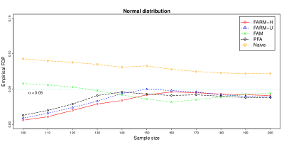
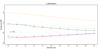
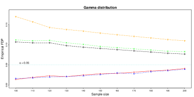
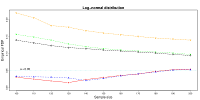
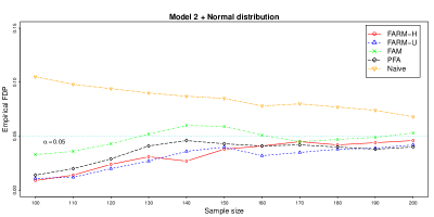
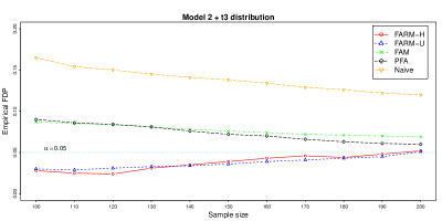
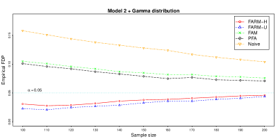
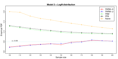
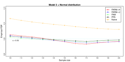
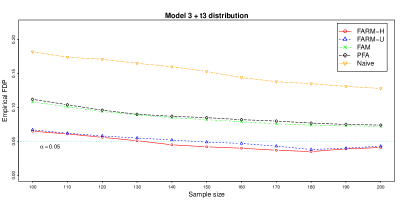
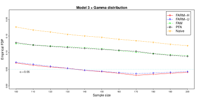
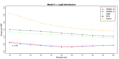
In this section, we compare the numerical performance of the five tests in respect of FDP/FDR control. We take $p=500$ and let $n$ gradually increase from 100 to 200. The empirical FDP is defined as the average false discovery proportion based on 200 simulations. At the prespecified level $\alpha=0.05$, Figure 4 displays the empirical FDP versus the sample size under Model 1. In the normal case, all the four factor-adjusted tests, FARM-H, FARM-$U$, FAM and PFA, have empirical FDPs controlled around or under $\alpha$. For heavy-tailed data, FARM-H and FARM-$U$ manage to control the empirical FDP under $\alpha$ for varying sample sizes; while FAM and PFA lead to much higher empirical FDPs, indicating more false discoveries. This phenomenon is in accord with our intuition that outliers can sometimes be mistakenly regarded as discoveries. The Naive method performs worst throughout all models and settings. Due to limitations of space, numerical results for Models 2 and 3 are given in Appendix E of the online supplement.

Figure 4: Empirical FDP versus sample size for the five tests at level $\alpha=0.05$. The data are generated from Model 1 with $p=500$ and sample size $n$ ranging from 100 to 200 with a step size of 10. The panels from top to bottom correspond to the four error distributions in Section 4.2.

5 Real data analysis

Oberthuer et al. (2006) analyzed the German Neuroblastoma Trials NB90-NB2004 (diagnosed between 1989 and 2004) and developed a gene expression based classifier. For 246 neuroblastoma patients, gene expressions over 10,707 probe sites were measured. The binary response variable is the 3-year event-free survival information of the patients (56 positive and 190 negative). We refer to Oberthuer et al. (2006) for a detailed description of the dataset. In this study, we divide the data into two groups, one with positive responses and the other with negative responses, and test the equality of gene expression levels at all the 10,707 probe sites simultaneously. To that end, we generalize the proposed FarmTest to the two-sample case by defining the following two-sample $t$-type statistics

$$T_{j}=\frac{(\widehat{\mu}_{1j}-\widehat{{\bm{b}}}_{1j}^{\mathrm{\scriptstyle T}}\widehat{\bm{f}}_{1})-(\widehat{\mu}_{2j}-\widehat{{\bm{b}}}_{2j}^{\mathrm{\scriptstyle T}}\widehat{\bm{f}}_{2})}{(\widehat{\sigma}_{1\varepsilon,jj}/56+\widehat{\sigma}_{2\varepsilon,jj}/190)^{1/2}},~{}~{}j=1,\ldots,10707,$$

where the subscripts 1 and 2 correspond to the positive and negative groups, respectively. Specifically, $\widehat{\mu}_{1j}$ and $\widehat{\mu}_{2j}$ are the robust mean estimators obtained from minimizing the empirical Huber risk (5), and $\widehat{{\bm{b}}}_{1j}$, $\widehat{{\bm{b}}}_{2j}$, $\widehat{\bm{f}}_{1}$ and $\widehat{\bm{f}}_{2}$ are robust estimators of the factors and loadings based on the $U$-type covariance estimator. In addition, $\widehat{\sigma}_{1\varepsilon,jj}$ and $\widehat{\sigma}_{2\varepsilon,jj}$ are the variance estimators defined in (27). As before, the robustification parameters are selected via five-fold cross-validation with their theoretically optimal orders taking into account.

Figure 5: Scree plots for positive and negative groups. The bars represent the proportion of variance explained by the top 20 principal components. The dots represent the corresponding eigenvalues in descending order.

Figure 6: Correlations among the first 100 genes before and after factor-adjustment. The pixel plots are the correlation matrices of the first 100 gene expressions. In the plots, the blue pixels represent the entries with correlation greater than 1/3 and the red pixels represent the entries with correlation smaller than -1/3.

Figure 7: Histogram of excess kurtosises for the gene expressions in positive and negative groups. The dashed line at 6 is the excess kurtosis of $t_{5}$-distribution.

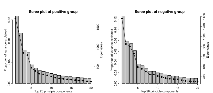
We use the eigenvalue ratio method (Lam and Yao, 2012; Ahn and Horenstein, 2013) to determine the number of factors. Let $\lambda_{k}(\widehat{\bm{\Sigma}})$ be the $k$-th largest eigenvalue of $\widehat{\bm{\Sigma}}$ and $K_{\max}$ a prespecified upper bound. The number of factors can then be estimated by

$$\widehat{K}=\arg\max\limits_{1\leq k\leq K_{\max}}\ {\lambda_{k}(\widehat{\bm{\Sigma}})}/{\lambda_{k+1}(\widehat{\bm{\Sigma}})}.$$

The eigenvalue ratio method suggests $K=4$ for both positive and negative groups. Figure 5 depicts scree plots of the top 20 eigenvalues for each group. The gene expressions in both groups are highly correlated. As an evidence, the top 4 principal components (PCs) explain 42.6% and 33.3% of the total variance for the positive and negative groups, respectively.

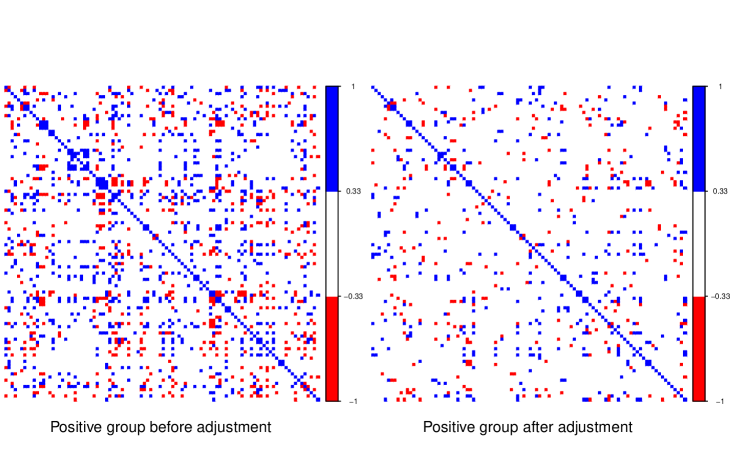
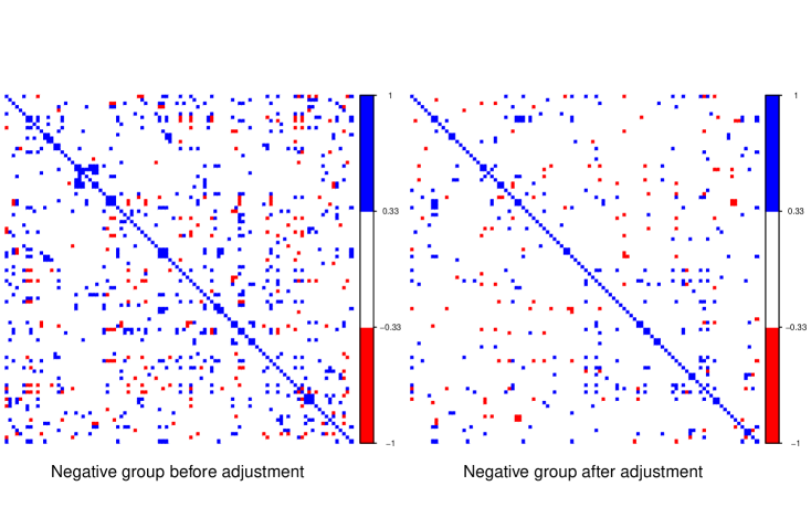
To demonstrate the importance of the factor-adjustment procedure, for each group, we plot the correlation matrices of the first 100 gene expressions before and after adjusting the top 4 PCs; see Figure 6. The blue and red pixels in Figure 6 represent the pairs of gene expressions whose absolute correlations are greater than 1/3. Therefore, after adjusting the top 4 PCs, the number of off-diagonal entries with strong correlations is significantly reduced in both groups. To be more specific, the number drops from 1452 to 666 for the positive group and from 848 to 414 for the negative group.

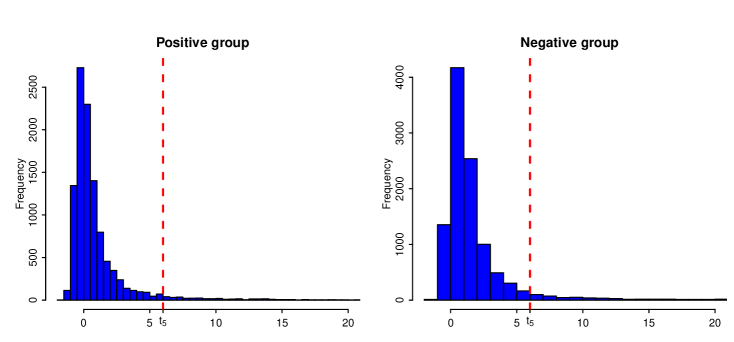
Another stylized feature of the data is that distributions of many gene expressions are heavy-tailed. To see this, we plot histograms of the excess kurtosis of the gene expressions in Figure 7. The left panel of the Figure 7 shows that 6518 gene expressions have positive excess kurtosis with 420 of them greater than 6. In other words, more than 60% of the gene expressions in the positive group have tails heavier than the normal distribution and about 4% are severely heavy tailed as their tails are fatter than the $t$-distribution with 5 degrees of freedom. Similarly, in the negative group, 9341 gene expressions exhibit positive excess kurtosis with 671 of them greater than 6. Such a heavy-tailed feature indicates the necessity of using robust methods to estimate the mean and covariance of the data.

We apply four tests, the two-sample FARM-H and FARM-$U$, the FAM test and the naive method, to this dataset. At level $\alpha=0.01$, the two-sample FARM-H and FARM-$U$ methods identify, respectively, 3912 and 3855 probes with different gene expressions, among which 3762 probes are identical. This shows an approximately 97% similarity in the two methods. The FAM and naive methods discover 3509 and 3236 probes, respectively. For this dataset, accounting for latent factor dependence indeed leads to different statistical conclusions. This visible discrepancy between the two robust methods and FAM highlights the importance of robustness and reflects the difference in power of detecting differently expressed probes. The effectiveness of factor adjustment is also highlighted in the discovery of significant genes.

6 Discussion and extensions

In this paper, we have developed a factor-adjusted multiple testing procedure (FarmTest) for large-scale simultaneous inference with dependent and heavy-tailed data, the key of which lies in a robust estimate of the false discovery proportion. The procedure has two attractive features: First, it incorporates dependence information to construct marginal test statistics. Intuitively, subtracting common factors out leads to higher signal-to-noise ratios, and therefore makes the resulting FDP control procedure more efficient and powerful. Second, to achieve robustness against heavy-tailed errors that may also be asymmetric, we used the adaptive Huber regression method (Fan et al., 2017; Zhou at al., 2018) to estimate the realized factors, factor loadings and variances. We believe that these two properties will have further applications to higher criticism for detecting sparse signals with dependent and non-Gaussian data; see Delaigle et al. (2011) for the independent case.

In other situations, it may be more instructive to consider the mixed effects regression modeling of the data (Friguet et al., 2009; Wang et al., 2017), that is, $X_{j}=\mu_{j}+\bm{\beta}_{j}^{\mathrm{\scriptstyle T}}\bm{Z}+\bm{b}_{j}^{\mathrm{\scriptstyle T}}\bm{f}+\varepsilon_{j}$ for $j=1,\ldots,p$, where $\bm{Z}\in\mathbb{R}^{q}$ is a vector of explanatory variables (e.g., treatment-control, phenotype, health trait), $\bm{\beta}_{j}$’s are $q\times 1$ vectors of unknown slope coefficients, and $\bm{f}$, $\bm{b}_{j}$’s and $\varepsilon_{j}$’s have the same meanings as in (1). Suppose we observe independent samples $(\bm{X}_{1},\bm{Z}_{1}),\ldots,(\bm{X}_{n},\bm{Z}_{n})$ from $(\bm{X},\bm{Z})$ satisfying

$$\bm{X}_{i}=\bm{\mu}+\bm{\Theta}\bm{Z}_{i}+\mathbf{B}\bm{f}_{i}+\bm{\varepsilon}_{i},\ \ i=1,\ldots,n,$$

where $\bm{\Theta}=(\bm{\beta}_{1},\ldots,\bm{\beta}_{p})^{\mathrm{\scriptstyle T}}\in\mathbb{R}^{p\times q}$. In this case, we have $\mathbb{E}(\bm{X}_{i}|\bm{Z}_{i})=\bm{\mu}+\bm{\Theta}\bm{Z}_{i}$ and $\textnormal{cov}(\bm{X}_{i}|\bm{Z}_{i})=\mathbf{B}\bm{\Sigma}_{f}\mathbf{B}^{\mathrm{\scriptstyle T}}+\bm{\Sigma}_{\varepsilon}$. The main issue in extending our methodology to such a mixed effects model is the estimation of $\bm{\Theta}$. For this, we construct robust estimators $(\widehat{\mu}_{j},\widehat{\bm{\beta}}_{j})$ of $(\mu_{j},\bm{\beta}_{j})$, defined as

$$(\widehat{\mu}_{j},\widehat{\bm{\beta}}_{j})\in\arg\min_{\mu\in\mathbb{R},\,\bm{\beta}_{j}\in\mathbb{R}^{q}}\sum_{i=1}^{n}\ell_{\tau_{j}}(X_{ij}-\mu-\bm{\beta}_{j}^{\mathrm{\scriptstyle T}}\bm{Z}_{i}),\ \ 1\leq j\leq p,$$

where $\tau_{j}$’s are robustification parameters. Taking $\widehat{\bm{\Theta}}=(\widehat{\bm{\beta}}_{1},\ldots,\widehat{\bm{\beta}}_{p})^{\mathrm{\scriptstyle T}}$, the FarmTest procedure in Section 2.2 can be directly applied with $\{\bm{X}_{i}\}_{i=1}^{n}$ replaced by $\{\bm{X}_{i}-\widehat{\bm{\Theta}}\bm{Z}_{i}\}_{i=1}^{n}$. However, because $\widehat{\bm{\Theta}}$ depends on $\{(\bm{X}_{i},\bm{Z}_{i})\}_{i=1}^{n}$, the adjusted data $\bm{X}_{1}-\widehat{\bm{\Theta}}\bm{Z}_{1},\ldots,\bm{X}_{n}-\widehat{\bm{\Theta}}\bm{Z}_{n}$ are no longer independent, which causes the main difficulty of extending the established theory in Section 3 to the current setting. One way to bypass this issue and to facilitate the theoretical analysis is the use of sample splitting as discussed in Appendix A of the online supplement. The FarmTest procedure for mixed effects models was also implemented in the R-package FarmTest (https://cran.r-project.org/web/packages/FarmTest).

Appendix

Appendix A Sample splitting

Our procedure described in Sections 3.2 and 3.3 consists of two parts, the calibration of a factor model (i.e. estimating $\mathbf{B}$ in equation (1)) and multiple inference. The construction of the test statistics, or equivalently, the $P$-values, relies on a “fine” estimate of $\bar{\bm{f}}$ based on the linear model in (25). In practice, $\bm{b}_{j}$’s are replaced by the fitted loadings $\widehat{\bm{b}}_{j}$’s using the methods in Section 3.2.

To avoid mathematical challenges caused by the reuse of the sample, we resort to the simple idea of sample splitting (Hartigan, 1969; Cox, 1975): half the data are used for calibrating a factor model and the other half are used for multiple inference. We refer to Rinaldo et al. (2016) for a modern look at inference based on sample splitting. Specifically, the steps are summarized below.

• Split the data $\mathcal{X}=\{\bm{X}_{1},\ldots,\bm{X}_{n}\}$ into two halves $\mathcal{X}_{1}$ and $\mathcal{X}_{2}$. For simplicity, we assume that the data are divided into two groups of equal size $m=n/2$.

• We use $\mathcal{X}_{1}$ to estimate $\bm{b}_{1},\ldots,\bm{b}_{p}$ using either the $U$-type method (Section 3.2.1) or the adaptive Huber method (Section 3.2.2). For simplicity, we focus on the latter and denote the estimators by $\widehat{\bm{b}}_{1}(\mathcal{X}_{1}),\ldots,\widehat{\bm{b}}_{p}(\mathcal{X}_{1})$.

• Proceed with the remain steps in the FarmTest procedure using the data in $\mathcal{X}_{2}$. Denote the resulting test statistics by ${T}_{1},\ldots,{T}_{p}$. For a given threshold $z\geq 0$, the corresponding FDP and its asymptotic expression are defined as

  $${{\rm FDP}}_{\rm sp}(z)={V}(z)/{R}(z)~{}\mbox{ and }~{}{\rm AFDP}_{\rm sp}(z)=2p\Phi(-z)/R(z),$$

  respectively, where ${V}(z)=\sum_{j\in\mathcal{H}_{0}}I(|{T}_{j}|\geq z)$, ${R}(z)=\sum_{1\leq j\leq p}I(|{T}_{j}|\geq z)$ and the subscript “sp” stands for sample splitting.

The purpose of sample splitting employed in the above procedure is to facilitate the theoretical analysis. The following result shows that the asymptotic FDP ${\rm AFDP}_{\rm sp}(z)$, constructed via sample splitting, provides a consistent estimate of ${{\rm FDP}}(z)$.

Theorem 6.

Suppose that Assumptions 1 (i)–(iv), Assumptions 2–4 hold. Let $\tau_{j}=a_{j}\omega_{n,p}$, $\tau_{jj}=a_{jj}\omega_{n,p}$ with $a_{j}\geq\sigma_{jj}^{1/2}$, $a_{jj}\geq\textnormal{var}(X_{j}^{2})^{1/2}$ for $j=1,\ldots,p$, and let $\gamma=\gamma_{0}\{p/\log(np)\}^{1/2}$ with $\gamma_{0}\geq\overline{\sigma}_{\varepsilon}$. Then, for any $z\geq 0$, $|{\rm AFDP}_{\rm sp}(z)-{{\rm FDP}}_{\rm sp}(z)|=o_{\mathbb{P}}(1)$ as $n,p\to\infty$.

Appendix B Derivation of (6)

For any $t$ and $a_{j}\geq\sigma_{jj}^{1/2}$, Lemma C.3 in Section C.1 shows that, conditionally on $\bm{f}_{i}$’s, the rescaled robust estimator $\sqrt{n}\,\widehat{\mu}_{j}$ with $\tau_{j}=a_{j}(n/t)^{1/2}$ satisfies

$$\sqrt{n}\,(\widehat{\mu}_{j}-\mu_{j}-\bm{b}^{\mathrm{\scriptstyle T}}_{j}\bar{\bm{f}}) =\bigg{\{}{\frac{1}{\sqrt{n}}\sum_{i=1}^{n}\ell^{\prime}_{\tau_{j}}(\bm{b}_{j}^{\mathrm{\scriptstyle T}}\bm{f}_{i}+\varepsilon_{ij})-\sqrt{n}\,\bm{b}^{\mathrm{\scriptstyle T}}_{j}\bar{\bm{f}}}\bigg{\}}+R_{1j},$$ (30)

where the remainder $R_{1j}$ satisfies $\mathbb{P}(|R_{1j}|\lesssim a_{j}n^{-1/2}t)\geq 1-3e^{-t}$. The stochastic term $n^{-1/2}\sum_{i=1}^{n}\ell^{\prime}_{\tau_{j}}(\bm{b}_{j}^{\mathrm{\scriptstyle T}}\bm{f}_{i}+\varepsilon_{ij})-\sqrt{n}\,\bm{b}^{\mathrm{\scriptstyle T}}_{j}\bar{\bm{f}}$ in (6) can be decomposed as

$$\frac{1}{\sqrt{n}}\sum_{i=1}^{n}\ell^{\prime}_{\tau_{j}}(\bm{b}_{j}^{\mathrm{\scriptstyle T}}\bm{f}_{i}+\varepsilon_{ij})-\sqrt{n}\,\bm{b}_{j}^{\mathrm{\scriptstyle T}}\bar{\bm{f}} =\underbrace{\frac{1}{\sqrt{n}}\sum_{i=1}^{n}\{\ell^{\prime}_{\tau_{j}}(\bm{b}_{j}^{\mathrm{\scriptstyle T}}\bm{f}_{i}+\varepsilon_{ij})-\mathbb{E}_{\bm{f}_{i}}\ell^{\prime}_{\tau_{j}}(\bm{b}_{j}^{\mathrm{\scriptstyle T}}\bm{f}_{i}+\varepsilon_{ij})\}}_{S_{j}}$$

$$\quad+\underbrace{\frac{1}{\sqrt{n}}\sum_{i=1}^{n}\{\mathbb{E}_{\bm{f}_{i}}\ell^{\prime}_{\tau_{j}}(\bm{b}_{j}^{\mathrm{\scriptstyle T}}\bm{f}_{i}+\varepsilon_{ij})-\bm{b}_{j}^{\mathrm{\scriptstyle T}}\bm{f}_{i}\}}_{R_{2j}},$$ (31)

where $\bar{\bm{f}}=n^{-1}\sum_{i=1}^{n}\bm{f}_{i}$ and $\mathbb{E}_{\bm{f}_{i}}(\cdot)=\mathbb{E}(\cdot|\bm{f}_{i})$ denotes the conditional expectation given $\bm{f}_{i}$. Under the finite fourth moment condition $\upsilon_{j}:=(\mathbb{E}\varepsilon_{j}^{4})^{1/4}<\infty$, it follows from Lemma C.4 that as long as $n\geq 4a_{j}^{-2}\max_{1\leq i\leq n}(\bm{b}_{j}^{\mathrm{\scriptstyle T}}\bm{f}_{i})^{2}t$,

$$|R_{2j}|\leq 8a_{j}^{-3}\upsilon_{j}^{4}\,n^{-1}t^{3/2}.$$ (32)

Given $\{\bm{f}_{i}\}_{i=1}^{n}$, $S_{j}$ in (B) is a sum of (conditionally) independent random variables with (conditional) mean zero. In addition, we note from (36) in Lemma C.4 that the (conditional) variance of $\ell^{\prime}_{\tau_{j}}(\bm{b}_{j}^{\rm T}\bm{f}_{i}+\varepsilon_{ij})$ given $\bm{f}_{i}$ satisfies $|\textnormal{var}_{\bm{f}_{i}}\{\ell^{\prime}_{\tau_{j}}(\bm{b}_{j}^{\rm T}\bm{f}_{i}+\varepsilon_{ij})\}-\sigma_{\varepsilon,jj}|\lesssim n^{-1}t$. Therefore, by the central limit theorem, the conditional distribution of $S_{j}$ given $\{\bm{f}_{i}\}_{i=1}^{n}$ is asymptotically normal with mean zero and variance $\sigma_{\varepsilon,jj}$ as long as $t=t(n,p)=o(n)$. This, together with (32) implies that, conditioning on $\{\bm{f}_{i}\}_{i=1}^{n}$, the distribution of $\sqrt{n}\,\widehat{\mu}_{j}$ is close to a normal distribution with mean $\sqrt{n}\,(\mu_{j}+\bm{b}_{j}^{{\rm T}}\bar{\bm{f}})$ and variance $\sigma_{\varepsilon,jj}$. Under the identifiability condition (2), $\sigma_{\varepsilon,jj}=\sigma_{jj}-\|\bm{b}_{j}\|_{2}^{2}$ for $j=1,\ldots,p$. We complete the proof.

Appendix C Proofs of main results

In this section, we present the proofs for Theorems 1–5 and Theorem 6, starting with some preliminary results whose proofs can be found in Section D. Recall that

$$w_{n,p}=\sqrt{\frac{n}{\log(np)}},$$

which will be frequently used in the sequel. Also, we use $c_{1},c_{2},\ldots$ and $C_{1},C_{2},\ldots$ to denote constants that are independent of $(n,p)$, which may take different values at each occurrence.

C.1 Preliminaries

For each $1\leq j\leq p$, define the zero-mean error variable $\xi_{j}=X_{j}-\mu_{j}$ and let $\mu_{j,\tau}=\mathop{\mathrm{argmin}}_{\theta\in\mathbb{R}}\mathbb{E}\ell_{\tau}(X_{j}-\theta)$ be the approximate mean, where $\ell_{\tau}(\cdot)$ is the Huber loss given in (5). Throughout, we use $\psi_{\tau}$ to denote the derivative of $\ell_{\tau}$, that is,

$$\psi_{\tau}(u)=\ell_{\tau}^{\prime}(u)=\min(|u|,\tau)\mathop{\mathrm{sgn}}(u),\ \ u\in\mathbb{R}.$$

Lemma C.1 provides an upper bound on the approximation bias $|\mu_{j}-\mu_{j,\tau}|$, whose proof is given in Section D.3.

Lemma C.1.

Let $1\leq j\leq p$ and assume that $\upsilon_{\kappa,j}=\mathbb{E}(|\xi_{j}|^{\kappa})<\infty$ for some $\kappa\geq 2$. Then, as long as $\tau>\sigma_{jj}^{1/2}$, we have

$$|\mu_{j,\tau}-\mu_{j}|\leq(1-\sigma_{jj}\tau^{-2})^{-1}\upsilon_{\kappa,j}\tau^{1-\kappa}.$$ (33)

The following concentration inequality is from Theorem 5 in Fan et al. (2017), showing that $\widehat{\mu}_{j}$ with a properly chosen robustification parameter $\tau$ exhibits sub-Gaussian tails when the underlying distribution has heavy tails with only finite second moment.

Lemma C.2.

For every $1\leq j\leq p$ and $t>0$, the estimator $\widehat{\mu}_{j}$ in (5) with $\tau=a(n/t)^{1/2}$ for $a\geq\sigma_{jj}^{1/2}$ satisfies $\mathbb{P}\{|\widehat{\mu}_{j}-\mu_{j}|\geq 4a(t/n)^{1/2}\}\leq 2e^{-t}$ as long as $n\geq 8t$.

The next result provides a nonasymptotic Bahadur representation for $\widehat{\mu}_{j}$. In particular, we show that when the second moment is finite, the remainder of the Bahadur representation for $\widehat{\mu}_{j}$ exhibits sub-exponential tails. The proof of Lemmas C.3–C.6 can be found respectively in Sections D.4–D.7.

Lemma C.3.

For every $1\leq j\leq p$ and for any $t\geq 1$, the estimator $\widehat{\mu}_{j}$ in (5) with $\tau=a(n/t)^{1/2}$ and $a\geq\sigma_{jj}^{1/2}$ satisfies that as long as $n\geq 8t$,

$$\bigg{|}\sqrt{n}\,(\widehat{\mu}_{j}-\mu_{j})-\frac{1}{\sqrt{n}}\sum_{i=1}^{n}\psi_{\tau}(\xi_{ij})\bigg{|}\leq C\frac{at}{\sqrt{n}}$$ (34)

with probability greater than $1-3e^{-t}$, where $\xi_{ij}=X_{ij}-\mu_{j}$ and $C>0$ is an absolute constant.

Under factor model (1), note that $\xi_{j}=\bm{b}_{j}^{\mathrm{\scriptstyle T}}\bm{f}+\varepsilon_{j}$ for every $j$. The following conclusion reveals that the differences between the first two (conditional) moments of $\xi_{j}$ and $\psi_{\tau}(\xi_{j})$ given $\bm{f}$ vanish faster if higher moments of $\varepsilon_{j}$ exist.

Lemma C.4.

Assume that $\mathbb{E}(|\varepsilon_{j}|^{\kappa})<\infty$ for some $1\leq j\leq p$ and $\kappa\geq 2$.

• On the event $\mathcal{G}_{j}:=\{|\bm{b}_{j}^{\mathrm{\scriptstyle T}}\bm{f}|<\tau\}$,

  $$|\mathbb{E}_{\bm{f}}\psi_{\tau}(\xi_{j})-\bm{b}_{j}^{\mathrm{\scriptstyle T}}\bm{f}|\leq\min\bigg{\{}\frac{\sigma_{\varepsilon,jj}}{\tau-|\bm{b}_{j}^{{\rm T}}\bm{f}|},\frac{\mathbb{E}|\varepsilon_{j}|^{\kappa}}{(\tau-|\bm{b}_{j}^{{\rm T}}\bm{f}|)^{\kappa-1}}\bigg{\}}$$ (35)

  almost surely. In addition, if $\kappa>2$, we have

  $$\sigma_{\varepsilon,jj}-\frac{\mathbb{E}(|\varepsilon_{j}|^{\kappa})}{(\tau-|\bm{b}_{j}^{\mathrm{\scriptstyle T}}\bm{f}|)^{\kappa-2}}\bigg{\{}\frac{2}{\kappa-2}+\frac{\mathbb{E}(|\varepsilon_{j}|^{\kappa})}{(\tau-|\bm{b}_{j}^{\mathrm{\scriptstyle T}}\bm{f}|)^{\kappa}}\bigg{\}}\leq{\rm var}_{\bm{f}}\{\psi_{\tau}(\xi_{j})\}\leq\sigma_{\varepsilon,jj}$$ (36)

  almost surely on $\mathcal{G}_{j}$.

• Assume that $\upsilon_{jk}:=\mathbb{E}(|\varepsilon_{j}|^{\kappa})\vee\mathbb{E}(|\varepsilon_{k}|^{\kappa})<\infty$ for some $1\leq j\neq k\leq p$ and $\kappa>2$. Then

  $$|\textnormal{cov}_{\bm{f}}(\psi_{\tau}(\xi_{j}),\psi_{\tau}(\xi_{k}))-\textnormal{cov}(\varepsilon_{j},\varepsilon_{k})|\leq C\max(\upsilon_{jk}\tau^{2-\kappa},\upsilon_{jk}^{2}\tau^{2-2\kappa})$$ (37)

  almost surely on $\mathcal{G}_{jk}:=\{|\bm{b}_{j}^{\mathrm{\scriptstyle T}}\bm{f}|\vee|\bm{b}_{k}^{\mathrm{\scriptstyle T}}\bm{f}|\leq\tau/2\}$, where $C>0$ is an absolute constant.

Lemma C.5.

Suppose that Assumption 1 holds. Then, for any $t>0$,

$$\mathbb{P}\{\|\sqrt{n}\bar{\bm{f}}\|_{2}>C_{1}A_{f}(K+t)^{1/2}\}\leq e^{-t},$$ (38)

$$\mathbb{P}\bigg{\{}\max_{1\leq i\leq n}\|\bm{f}_{i}\|_{2}>C_{1}A_{f}(K+\log n+t)^{1/2}\bigg{\}}\leq e^{-t},$$ (39)

$$\mbox{ and }~{}\mathbb{P}[\|\widehat{\bm{\Sigma}}_{f}-\mathbf{I}_{K}\|_{2}>C_{2}\max\{A_{f}^{2}n^{-1/2}(K+t)^{1/2},A_{f}^{4}n^{-1}(K+t)\}]\leq 2e^{-t},$$ (40)

where $\bar{\bm{f}}=n^{-1}\sum_{i=1}^{n}\bm{f}_{i}$, $\widehat{\bm{\Sigma}}_{f}=n^{-1}\sum_{i=1}^{n}\bm{f}_{i}\bm{f}_{i}^{\mathrm{\scriptstyle T}}$ and $C_{1},C_{2}>0$ are absolute constants.

The following lemma provides an $\ell_{\infty}$-error bound for estimating the eigenvectors $\overline{\bm{v}}_{\ell}$’s of $\mathbf{B}^{\mathrm{\scriptstyle T}}\mathbf{B}$. The proof is based on an $\ell_{\infty}$ eigenvector perturbation bound developed in Fan et al. (2018) and is given in Appendix D.

Lemma C.6.

Suppose Assumption 2 holds. Then we have

$$\max_{1\leq\ell\leq K}|\widetilde{\lambda}_{\ell}-\overline{\lambda}_{\ell}|\leq p\|\widehat{\bm{\Sigma}}_{{\rm H}}-\bm{\Sigma}\|_{\max}+\|\bm{\Sigma}_{\varepsilon}\|$$ (41)

$$\mbox{ and }~{}\max_{1\leq\ell\leq K}\|\widehat{\bm{v}}_{\ell}-\overline{\bm{v}}_{\ell}\|_{\infty}\leq C(p^{-1/2}\|\widehat{\bm{\Sigma}}_{{\rm H}}-\bm{\Sigma}\|_{\max}+p^{-1}\|\bm{\Sigma}_{\varepsilon}\|),$$ (42)

where $C>0$ is a constant independent of $(n,p)$.

C.2 Proof of Theorem 1

To prove (15) and (16), we will derive the following stronger results that

$$p_{0}^{-1}V(z) =2\Phi(-z)+O_{\mathbb{P}}\{p^{-\kappa_{1}/2}+w_{n,p}^{-1/2}+n^{-1/2}\log(np)\}$$ (43)

$$\mbox{ and }~{}p^{-1}R(z) =\frac{1}{p}\sum_{j=1}^{p}\bigg{\{}\Phi\bigg{(}-z+\frac{\sqrt{n}\mu_{j}}{\sqrt{\sigma_{\varepsilon,jj}}}\bigg{)}+\Phi\bigg{(}-z-\frac{\sqrt{n}\mu_{j}}{\sqrt{\sigma_{\varepsilon,jj}}}\bigg{)}\bigg{\}}$$

$$\quad~{}+O_{\mathbb{P}}\{p^{-\kappa_{1}/2}+w_{n,p}^{-1/2}+n^{-1/2}\log(np)\}$$ (44)

uniformly over $z\geq 0$ as $n,p\to\infty$, where $w_{n,p}=\sqrt{n/\log(np)}$.

For $1\leq j\leq p$ and $t\geq 1$, set $\tau_{j}=a_{j}\sqrt{n/t}$ with $a_{j}\geq\sigma^{1/2}_{jj}$. By Lemma C.3, for every $j\in\mathcal{H}_{0}$ so that $\mu_{j}=0$,

$$|T_{j}^{\circ}-\sigma_{\varepsilon,jj}^{-1/2}(S_{j}+R_{2j})|\leq c_{1}\frac{a_{j}t}{\sqrt{\sigma_{\varepsilon,jj}n}}$$ (45)

with probability greater than $1-3e^{-t}$ as long as $n\geq 8t$, where

$$S_{j}=\frac{1}{\sqrt{n}}\sum_{i=1}^{n}S_{ij}~{}\mbox{ with }~{}S_{ij}:=\psi_{\tau_{j}}(\bm{b}_{j}^{\mathrm{\scriptstyle T}}\bm{f}_{i}+\varepsilon_{ij})-\mathbb{E}_{\bm{f}_{i}}\psi_{\tau_{j}}(\bm{b}_{j}^{\mathrm{\scriptstyle T}}\bm{f}_{i}+\varepsilon_{ij}),$$ (46)

$R_{2j}=n^{-1/2}\sum_{i=1}^{n}\{\mathbb{E}_{\bm{f}_{i}}\psi_{\tau_{j}}(\bm{b}_{j}^{\mathrm{\scriptstyle T}}\bm{f}_{i}+\varepsilon_{ij})-\bm{b}_{j}^{\mathrm{\scriptstyle T}}\bm{f}_{i}\}$. For $j=1,\ldots,p$, denote by $\mathcal{E}_{1j}(t)$ the event that (45) holds. Define $\mathcal{E}_{1}(t)=\bigcap_{j=1}^{p}\mathcal{E}_{1j}(t)$, on which it holds

$$\sum_{j\in\mathcal{H}_{0}}I\bigg{(}|T_{0j}|\geq z+\frac{c_{1}a_{j}t}{\sqrt{\sigma_{\varepsilon,jj}n}}\bigg{)}\leq V(z)\leq\sum_{j\in\mathcal{H}_{0}}I\bigg{(}|T_{0j}|\geq z-\frac{c_{1}a_{j}t}{\sqrt{\sigma_{\varepsilon,jj}n}}\bigg{)},$$ (47)

where $T_{0j}:=\sigma_{\varepsilon,jj}^{-1/2}(S_{j}+R_{2j})$. Next, let $\mathcal{E}_{2}(t)$ denote the event on which the following hold:

$$\|\sqrt{n}\bar{\bm{f}}\|_{2}\leq C_{1}A_{f}(K+t)^{1/2},\ \ \max_{1\leq i\leq n}\|\bm{f}_{i}\|_{2}\leq C_{1}A_{f}(K+\log n+t)^{1/2},$$

$$\mbox{and }~{}\|\widehat{\bm{\Sigma}}_{f}-\mathbf{I}_{K}\|_{2}\leq C_{2}\max\{A_{f}^{2}n^{-1/2}(K+t)^{1/2},A_{f}^{4}n^{-1}(K+t)\}.$$

From Lemmas C.3, C.5 and the union bound, it follows that

$$\mathbb{P}\{\mathcal{E}_{1}(t)^{{\rm c}}\}\leq pe^{-t}~{}~{}\mbox{ and }~{}~{}\mathbb{P}\{\mathcal{E}_{2}(t)^{{\rm c}}\}\leq 4e^{-t}.$$

With the above preparations, we are ready to prove (43). The proof of (44) follows the same argument and therefore is omitted. Note that, on the event $\mathcal{E}_{2}(t)$,

$$\max_{1\leq i\leq n}|\bm{b}_{j}^{\mathrm{\scriptstyle T}}\bm{f}_{i}|\leq C_{1}A_{f}\|\bm{b}_{j}\|_{2}(K+\log n+t)^{1/2}~{}\mbox{ for all }1\leq j\leq p.$$

By the definition of $\tau_{j}$’s,

$$\max_{1\leq i\leq n}|\bm{b}_{j}^{\mathrm{\scriptstyle T}}\bm{f}_{i}|\leq\tau_{j}/2~{}\mbox{ for all }j=1,\ldots,p,$$ (48)

as long as $n\geq 4(C_{1}A_{f})^{2}(K+\log n+t)t$. This, together with Lemma C.5, implies $|R_{2j}|\leq 8a_{j}^{-3}\upsilon_{j}^{4}\,n^{-1}t^{3/2}$ almost surely on $\mathcal{E}_{2}(t)$ for all sufficiently large $n$. Moreover, taking (47) into account we obtain that, almost surely on the event $\mathcal{E}_{1}(t)\cap\mathcal{E}_{2}(t)$,

$$\sum_{j\in\mathcal{H}_{0}}I(|\sigma_{\varepsilon,jj}^{-1/2}S_{j}|\geq z+c_{2}n^{-1/2}t)\leq V(z)\leq\sum_{j\in\mathcal{H}_{0}}I(|\sigma_{\varepsilon,jj}^{-1/2}S_{j}|\geq z-c_{2}n^{-1/2}t)$$ (49)

as long as $n\gtrsim(K+t)t$. For $x\in\mathbb{R}$, define

$$\widetilde{V}_{+}(x)=\sum_{j\in\mathcal{H}_{0}}I(\sigma_{\varepsilon,jj}^{-1/2}S_{j}\geq x)~{}\mbox{ and }~{}\widetilde{V}_{-}(x)=\sum_{j\in\mathcal{H}_{0}}I(\sigma_{\varepsilon,jj}^{-1/2}S_{j}\leq-x),$$

so that (49) can be written as

$$p_{0}^{-1}\{\widetilde{V}_{+}(z+c_{2}n^{-1/2}t)+\widetilde{V}_{-}(z+c_{2}n^{-1/2}t)\}$$

$$\leq p_{0}^{-1}V(z)\leq p_{0}^{-1}\{\widetilde{V}_{+}(z-c_{2}n^{-1/2}t)+\widetilde{V}_{-}(z-c_{2}n^{-1/2}t)\}.$$ (50)

Therefore, to prove (43) it suffices to focus on $\widetilde{V}_{+}$ and $\widetilde{V}_{-}$.

Observe that, conditional on $\mathcal{F}_{n}:=\{\bm{f}_{1},\ldots,\bm{f}_{n}\}$, $I(\sigma_{\varepsilon,11}^{-1/2}S_{1}\geq z),\ldots,I(\sigma_{\varepsilon,pp}^{-1/2}S_{p}\geq z)$ are weakly correlated random variables. Define

$$Y_{j}=I(\sigma_{\varepsilon,jj}^{-1/2}S_{j}\geq z)~{}\mbox{ and }~{}P_{j}=\mathbb{P}(\sigma_{\varepsilon,jj}^{-1/2}S_{j}\geq z|\mathcal{F}_{n})$$

for $j=1,\ldots,p$, and note that

$$\textnormal{var}\bigg{(}\frac{1}{p_{0}}\sum_{j\in\mathcal{H}_{0}}Y_{j}\bigg{|}\mathcal{F}_{n}\bigg{)} =\frac{1}{p_{0}^{2}}\sum_{j\in\mathcal{H}_{0}}\textnormal{var}(Y_{j}|\mathcal{F}_{n})+\frac{1}{p_{0}^{2}}\sum_{j,k\in\mathcal{H}_{0}:j\neq k}\textnormal{cov}(Y_{j},Y_{k}|\mathcal{F}_{n})$$

$$\leq\frac{1}{4p_{0}}+\frac{1}{p_{0}^{2}}\sum_{j,k\in\mathcal{H}_{0}:j\neq k}\{\mathbb{E}(Y_{j}Y_{k}|\mathcal{F}_{n})-P_{j}P_{k}\}$$ (51)

almost surely. In the following, we will study $P_{j}$ and $\mathbb{E}(Y_{j}Y_{k}|\mathcal{F}_{n})$ separately, starting with the former. Conditional on $\mathcal{F}_{n}$, $S_{j}$ is a sum of independent zero-mean random variables with conditional variance $s^{2}_{j}:=\textnormal{var}(S_{j}|\mathcal{F}_{n})=n^{-1}\sum_{i=1}^{n}s_{ij}^{2}$ where $s_{ij}^{2}:=\textnormal{var}(S_{ij}|\mathcal{F}_{n})$. Let $G\sim\mathcal{N}(0,1)$ be a standard normal random variable independent of the data. By the Berry-Esseen inequality,

$$\sup_{x\in\mathbb{R}}|\mathbb{P}(\sigma_{\varepsilon,jj}^{-1/2}S_{j}\leq x|\mathcal{F}_{n})-\mathbb{P}(s_{j}\sigma_{\varepsilon,jj}^{-1/2}G\leq x|\mathcal{F}_{n})|$$

$$\lesssim\frac{1}{(ns_{j})^{3/2}}\sum_{i=1}^{n}\mathbb{E}_{\bm{f}_{i}}|\psi_{\tau_{j}}(\bm{b}_{j}^{\mathrm{\scriptstyle T}}\bm{f}_{i}+\varepsilon_{ij})|^{3}\lesssim\frac{1}{(ns_{j})^{3/2}}\sum_{i=1}^{n}(|\bm{b}_{j}^{\mathrm{\scriptstyle T}}\bm{f}_{i}|^{3}+\mathbb{E}|\varepsilon_{ij}|^{3})$$ (52)

almost surely, where conditional on $\mathcal{F}_{n}$, $s_{j}\sigma_{\varepsilon,jj}^{-1/2}G\sim\mathcal{N}(0,s_{j}^{2}\sigma_{\varepsilon,jj}^{-1})$. Since $\max_{1\leq i\leq n}|\bm{b}_{j}^{\mathrm{\scriptstyle T}}\bm{f}_{i}|\leq\tau_{j}/2$ for all $1\leq j\leq p$ on $\mathcal{E}_{2}(t)$, applying Lemma C.4 with $\kappa=4$ yields

$$\sigma_{\varepsilon,jj}-4a_{j}^{-2}\upsilon_{j}^{4}(1+16a_{j}^{-4}\upsilon_{j}^{4}\,n^{-2}t^{2})n^{-1}t\leq s^{2}_{j}\leq\sigma_{\varepsilon,jj}$$ (53)

almost surely on the event $\mathcal{E}_{2}(t)$. Using (53) and Lemma A.7 in the supplement of Spokoiny and Zhilova (2015), we get

$$\sup_{x\in\mathbb{R}}|\mathbb{P}(s_{j}\sigma_{\varepsilon,jj}^{-1/2}G\leq x|\mathcal{F}_{n})-\Phi(x)|\lesssim a_{j}^{-2}\upsilon_{j}^{4}\,n^{-1}t$$ (54)

almost surely on $\mathcal{E}_{2}(t)$ as long as $n\gtrsim(K+t)t$. Putting (52) and (54) together we conclude that, almost surely on $\mathcal{E}_{2}(t)$,

$$\max_{1\leq j\leq p}|P_{j}-\Phi(-z)|\lesssim n^{-1/2}(K+\log n+t)^{1/2}$$ (55)

uniformly for all $z\geq 0$ as long as $n\gtrsim(K+t)t$.

Next we consider the joint probability $\mathbb{E}(Y_{j}Y_{k}|\mathcal{F}_{n})=\mathbb{P}(\sigma_{\varepsilon,jj}^{-1/2}S_{j}\geq z,\sigma_{\varepsilon,kk}^{-1/2}S_{k}\geq z|\mathcal{F}_{n})$ for a fixed pair $(j,k)$ satisfying $1\leq j\neq k\leq p$. Define bivariate random vectors $\bm{\xi}_{i}=(s_{j}^{-1}S_{ij},s_{k}^{-1}S_{ik})^{\mathrm{\scriptstyle T}}$ for $i=1,\ldots,n$. Observe that $\bm{\xi}_{1},\ldots,\bm{\xi}_{n}$ are conditionally independent random vectors given $\mathcal{F}_{n}$. Denote by $\mathbf{A}=(a_{uv})_{1\leq u,v\leq 2}$ the covariance matrix of $n^{-1/2}\sum_{i=1}^{n}\bm{\xi}_{i}=(s_{j}^{-1}S_{j},s_{k}^{-1}S_{k})^{\mathrm{\scriptstyle T}}$ given $\mathcal{F}_{n}$ such that

$$a_{11}=a_{22}=1~{}~{}\mbox{ and }~{}~{}a_{12}=a_{21}=\frac{1}{ns_{j}s_{k}}\sum_{i=1}^{n}\textnormal{cov}_{\bm{f}_{i}}(S_{ij},S_{ik}).$$

By Lemma C.4 and (53), we have $|a_{12}-r_{\varepsilon,jk}|\lesssim n^{-1}t$ almost surely on $\mathcal{E}_{2}(t)$. Therefore, the matrix $\mathbf{A}$ is positive definite almost surely on $\mathcal{E}_{2}(t)$ whenever $n\gtrsim t$. Let $\bm{G}=(G_{1},G_{2})^{\mathrm{\scriptstyle T}}$ be a Gaussian random vector with $\mathbb{E}(\bm{G})={\mathbf{0}}$ and $\textnormal{cov}(\bm{G})=\mathbf{A}$. Then, applying Theorem 1.1 in Bentkus (2005), a multivariate Berry-Esseen bound, to $n^{-1/2}\sum_{i=1}^{n}\bm{\xi}_{i}$ gives

$$\sup_{x,y\in\mathbb{R}}|\mathbb{P}(s_{j}^{-1}S_{j}\geq x,s_{k}^{-1}S_{k}\geq y|\mathcal{F}_{n})-\mathbb{P}(G_{1}\geq x,G_{2}\geq y)|$$

$$\lesssim\frac{1}{n^{3/2}}\sum_{i=1}^{n}\mathbb{E}(\|\mathbf{A}^{-1/2}\bm{\xi}_{i}\|_{2}^{3})\lesssim\frac{1}{\sqrt{n}}+\frac{1}{n^{3/2}}\sum_{i=1}^{n}(|\bm{b}_{j}^{\mathrm{\scriptstyle T}}\bm{f}_{i}|^{3}+|\bm{b}_{k}^{\mathrm{\scriptstyle T}}\bm{f}_{i}|^{3})$$

almost surely on $\mathcal{E}_{2}(t)$. Taking $x=s_{j}^{-1}\sigma_{\varepsilon,jj}^{1/2}\,z$ and $y=s_{k}^{-1}\sigma_{\varepsilon,kk}^{1/2}\,z$ implies

$$|\mathbb{E}(Y_{j}Y_{k}|\mathcal{F}_{n})-\mathbb{P}(G_{1}\geq s_{j}^{-1}\sigma_{\varepsilon,jj}^{1/2}\,z,\, G_{2}\geq s_{k}^{-1}\sigma_{\varepsilon,kk}^{1/2}\,z|\mathcal{F}_{n})|$$

$$\lesssim\frac{1}{\sqrt{n}}+\frac{1}{n^{3/2}}\sum_{i=1}^{n}(|\bm{b}_{j}^{\mathrm{\scriptstyle T}}\bm{f}_{i}|^{3}+|\bm{b}_{k}^{\mathrm{\scriptstyle T}}\bm{f}_{i}|^{3}).$$ (56)

For the bivariate Gaussian random vector $(G_{1},G_{2})^{\mathrm{\scriptstyle T}}$ with $a_{12}=\textnormal{cov}(G_{1},G_{2})$, it follows from Corollary 2.1 in Li and Shao (2002) that, for any $x,y\in\mathbb{R}$,

$$|\mathbb{P}(G_{1}\geq x,G_{2}\geq y)-\{1-\Phi(x)\}\{1-\Phi(y)\}|\leq\frac{|a_{12}|}{4}\exp\bigg{\{}-\frac{x^{2}+y^{2}}{2(1+|a_{12}|)}\bigg{\}}\leq\frac{|a_{12}|}{4}.$$

This, together with the Gaussian comparison inequality (54) gives

$$|\mathbb{P}(G_{1}\geq s_{j}^{-1}\sigma_{\varepsilon,jj}^{1/2}\,z,G_{2}\geq s_{k}^{-1}\sigma_{\varepsilon,kk}^{1/2}\,z|\mathcal{F}_{n})-\Phi(-z)^{2}|\lesssim|r_{\varepsilon,jk}|+n^{-1}t$$ (57)

almost surely on $\mathcal{E}_{2}(t)$ as long as $n\gtrsim(K+t)t$.

Consequently, it follows from (51), (55), (56), (57) and Assumption 1 that

$$\mathbb{E}[\{p_{0}^{-1}\widetilde{V}_{+}(z) -\Phi(-z)\}^{2}|\mathcal{F}_{n}]\lesssim p^{-\kappa_{1}}+n^{-1/2}(K+\log n+t)^{1/2}$$ (58)

almost surely on $\mathcal{E}_{2}(t)$ as long as $n\gtrsim(K+t)t$. A similar bound can be obtained for $\mathbb{E}[\{p_{0}^{-1}\widetilde{V}_{-}(z)-\Phi(-z)\}^{2}|\mathcal{F}_{n}]$. Recall that $\mathbb{P}\{\mathcal{E}_{1}(t)\cap\mathcal{E}_{2}(t)\}\geq 1-(p+4)e^{-t}$ whenever $n\geq 8t$. Finally, taking $t=\log(np)$ in (50) and (58) proves (43). ∎

C.3 Proof of Proposition 1

To begin with, observe that

$$\bigg{|}\widetilde{T}_{j}-\sqrt{\frac{n}{\widetilde{\sigma}_{\varepsilon,jj}}}(\widehat{\mu}_{j}-\bm{b}_{j}^{\mathrm{\scriptstyle T}}\bar{\bm{f}}\,)\bigg{|}=\sqrt{\frac{n}{\widetilde{\sigma}_{\varepsilon,jj}}}|(\widetilde{\bm{b}}_{j}-\bm{b}_{j})^{\mathrm{\scriptstyle T}}\bar{\bm{f}}|\leq\sqrt{\frac{n}{\widetilde{\sigma}_{\varepsilon,jj}}}\|\bar{\bm{f}}\|_{2}\|\widetilde{\bm{b}}_{j}-\bm{b}_{j}\|_{2},$$

$$\bigg{|}\sqrt{\frac{n}{\widetilde{\sigma}_{\varepsilon,jj}}}(\widehat{\mu}_{j}-\bm{b}_{j}^{\mathrm{\scriptstyle T}}\bar{\bm{f}}\,)-T^{\circ}_{j}\bigg{|}\leq\bigg{|}\frac{1}{\sqrt{\widetilde{\sigma}_{\varepsilon,jj}}}-\frac{1}{\sqrt{\sigma_{\varepsilon,jj}}}\bigg{|}(|\sqrt{n}\,\widehat{\mu}_{j}|+\|\bm{b}_{j}\|_{2}\|\sqrt{n}\bar{\bm{f}}\|_{2}).$$

By Lemma C.5, $\|\sqrt{n}\bar{\bm{f}}\|_{2}\lesssim(K+\log n)^{1/2}$ with probability greater than $1-n^{-1}$. Moreover, it follows from Lemma C.2 that $\max_{1\leq j\leq p}|\widehat{\mu}_{j}-\mu_{j}|\lesssim\{\log(np)\}^{1/2}n^{-1/2}$ with probability at least $1-2n^{-1}$. Putting the above calculations together, we conclude that

$$\max_{j\in\mathcal{H}_{0}}|\widetilde{T}_{j}-T_{j}^{\circ}|\lesssim\frac{\log(np)}{\sqrt{n}}+(K+\log n)^{1/2}\max_{1\leq j\leq p}(\|\widetilde{\bm{b}}_{j}-\bm{b}_{j}\|_{2}+|\widetilde{\sigma}_{jj}-\sigma_{jj}|)$$

with probability at least $1-3n^{-1}$. Combining this with the proof of Theorem 1 and condition (17) implies $p_{0}^{-1}\widetilde{V}(z)=2\Phi(-z)+o_{\mathbb{P}}(1)$. Similarly, it can be proved that (44) holds with $R(z)$ replaced by $\widetilde{R}(z)$. The conclusion follows immediately. ∎

C.4 Proof of Theorem 2

We first note that the $\widehat{\bm{\Sigma}}=\widehat{\bm{\Sigma}}_{U}$ defined is a $U$-statistic of order two. For simplicity, let $\mathcal{C}$ denote the set of $\binom{n}{2}$ distinct pairs $(i_{1},i_{2})$ satisfying $1\leq i_{1}<i_{2}\leq n$. Let $h(\bm{X}_{i},\bm{X}_{j})=2^{-1}(\bm{X}_{i}-\bm{X}_{j})(\bm{X}_{i}-\bm{X}_{j})^{\mathrm{\scriptstyle T}}$ and $Y_{ij}=\psi_{\tau}(h(\bm{X}_{i},\bm{X}_{j}))=\tau\psi_{1}(\tau^{-1}h(\bm{X}_{i},\bm{X}_{j}))$, such that

$$\widehat{\bm{\Sigma}}=\frac{1}{\binom{n}{2}}\sum_{(i,j)\in\mathcal{C}}Y_{ij}.$$

We now rewrite the $U$-statistic $\widehat{\bm{\Sigma}}$ as an average of dependent averages of identically and independently distributed random matrices. Define $k=[n/2]$, the greatest integer $\leq n/2$ and define

$$W_{(1,\ldots,n)}=k^{-1}(Y_{12}+Y_{23}+\ldots+Y_{2k-1,2k}).$$

Let $\mathcal{P}$ denote the class of all $n!$ permutations of $(1,\ldots,n)$ and $\pi=(i_{1},\ldots,i_{n}):\{1,\ldots,n\}\mapsto\{1,\ldots,n\}$ be a permutation, i.e. $\pi(k)=i_{k}$ for $k=1,\ldots,n$. Then it can be shown that

$$\widehat{\bm{\Sigma}}=\frac{1}{n!}\sum_{\pi\in\mathcal{P}}W_{\pi}.$$

Using the convexity of maximum eigenvalue function $\lambda_{\max}(\cdot)$ along with the convexity of the exponential function, we obtain

$$\exp\{\lambda_{\max}(\widehat{\bm{\Sigma}}-\bm{\Sigma})/\tau\}\leq\frac{1}{n!}\sum_{\pi\in\mathcal{P}}\exp\{\lambda_{\max}(W_{\pi}-\bm{\Sigma})/\tau\}.$$

Combining this with Chebyshev’s inequality delivers

$$\mathbb{P}\{\lambda_{\max}(\widehat{\bm{\Sigma}}-\bm{\Sigma})\geq t/\sqrt{n}\}$$

$$=\mathbb{P}\Big{[}\exp\{\lambda_{\max}(k\widehat{\bm{\Sigma}}-k\bm{\Sigma})/\tau\}\geq\exp\{kt/(\tau\sqrt{n}\,)\}\Big{]}$$

$$\leq e^{-{kt}/(\tau\sqrt{n})}\frac{1}{n!}\sum_{\pi\in\mathcal{P}}\mathbb{E}\exp\{\lambda_{\max}(kW_{\pi}-k\bm{\Sigma})/\tau\}$$

$$\leq e^{-{kt}/(\tau\sqrt{n})}\frac{1}{n!}\sum_{\pi\in\mathcal{P}}\mathbb{E}\mathop{\mathrm{tr}}\exp\{(kW_{\pi}-k\bm{\Sigma})/\tau\},$$

where we use the property $e^{\lambda_{\max}(\mathbf{A})}\leq\mathop{\mathrm{tr}}e^{\mathbf{A}}$ in the last inequality. For a given permutation $\pi=(i_{1},\ldots,i_{n})\in\mathcal{P}$, we write $Y_{\pi j}=Y_{i_{2j-1}i_{2j}}$ and $H_{\pi j}=h(\bm{X}_{i_{2j-1}},\bm{X}_{i_{2j}})$ with $\mathbb{E}H_{\pi j}=\bm{\Sigma}$. We then rewrite $W_{\pi}$ as $W_{\pi}=k^{-1}(Y_{\pi 1}+\ldots+Y_{\pi k})$, where $Y_{\pi j}$’s are mutually independent. Before proceeding, we introduce the following lemma whose proof is based on elementary calculations.

Lemma C.7.

For any $\tau>0$ and $x\in\mathbb{R}$, we have $\psi_{\tau}(x)=\tau\psi_{1}(x/\tau)$ and

$$-\log(1-x+x^{2})\leq\psi_{1}(x)\leq\log(1+x+x^{2})~{}\mbox{ for all }x\in\mathbb{R}.$$

From Lemma C.7 we see that the matrix $Y_{\pi j}$ can be bounded as

$$-\log(\mathbf{I}_{p}-H_{\pi j}/\tau+H^{2}_{\pi j}/\tau^{2})\leq Y_{\pi j}/\tau\leq\log(\mathbf{I}_{p}+H_{\pi j}/\tau+H_{\pi j}^{2}/\tau^{2}).$$

Using this property we can bound $\mathbb{E}\exp\{\mathop{\mathrm{tr}}(kW_{\pi}-k\bm{\Sigma})/\tau\}$ by

$$\mathbb{E}_{[k-1]}\mathbb{E}_{k}\mathop{\mathrm{tr}}\exp\Bigg{\{}\sum_{j=1}^{k-1}{Y_{\pi j}}-(k/\tau)\bm{\Sigma}+{Y_{\pi k}}\Bigg{\}}$$

$$\hskip 28.45274pt\leq\mathbb{E}_{[k-1]}\mathbb{E}_{k}\mathop{\mathrm{tr}}\exp\Bigg{\{}\sum_{j=1}^{k-1}{Y_{\pi j}}-(k/\tau)\bm{\Sigma}+\log(\mathbf{I}_{p}+H_{\pi j}/\tau+H_{\pi j}^{2}/\tau^{2})\Bigg{\}}$$ (59)

To further bound the right-hand side of (C.4), we follow a similar argument as in Minsker (2016). The following lemma, which is taken from Lieb (2002), is commonly referred to as the Lieb’s concavity theorem.

Lemma C.8.

For any symmetric matrix $H\in\mathbb{R}^{d\times d}$, the function

$$f(A)=\mathop{\mathrm{tr}}\exp(H+\log A),\ \ A\in\mathbb{R}^{d\times d}$$

is concave over the set of all positive definite matrices.

Applying Lemma C.8 repeatedly along with Jensen’s inequality, we obtain

$$\mathbb{E}\{\mathop{\mathrm{tr}}\exp(kW_{\pi}-k\bm{\Sigma})/\tau\} \leq\mathbb{E}\mathop{\mathrm{tr}}\exp\Bigg{\{}\sum_{j=1}^{k-1}{Y_{\pi j}}-(k/\tau)\bm{\Sigma}+\log(\mathbf{I}_{p}+\mathbb{E}H_{\pi k}/\tau+\mathbb{E}H_{\pi k}^{2}/\tau^{2})\Bigg{\}}$$

$$\leq\mathop{\mathrm{tr}}\exp\Bigg{\{}\sum_{j=1}^{k}\log(\mathbf{I}_{p}+\mathbb{E}H_{\pi j}/\tau+\mathbb{E}H_{\pi j}^{2}/\tau^{2})-(k/\tau)\bm{\Sigma}\Bigg{\}}$$

$$\leq\mathop{\mathrm{tr}}\exp\Bigg{(}\sum_{j=1}^{k}\mathbb{E}H_{\pi k}^{2}/\tau^{2}\Bigg{)},$$

where we use the inequality $\log(1+x)\leq x$ for $x>-1$ in the last step. The following lemma gives an explicit form for $v^{2}:=\|\mathbb{E}H_{\pi k}^{2}\|_{2}$.

Lemma C.9.

We have

$$\|\mathbb{E}h^{2}(\bm{X}_{1},\bm{X}_{2})\|_{2}=\frac{1}{2}\Big{\|}\mathbb{E}\{(\bm{X}-\bm{\mu})(\bm{X}-\bm{\mu})^{\mathrm{\scriptstyle T}}\}^{2}+\mathop{\mathrm{tr}}(\bm{\Sigma})\bm{\Sigma}+2\bm{\Sigma}^{2}\Big{\|}.$$

Proof of Lemma C.9.

Write $\bm{X}=\bm{X}_{1}$ and $\bm{Y}=\bm{X}_{2}$. Without loss of generality, assume that $\mathbb{E}(\bm{X})\!=\!\mathbb{E}(\bm{Y})\!=\!{\bf 0}$. Let $H_{1}=\bm{X}\bm{X}^{\mathrm{\scriptstyle T}},~{}H_{2}=\bm{Y}\bm{Y}^{\mathrm{\scriptstyle T}},~{}H_{12}=\bm{X}\bm{Y}^{\mathrm{\scriptstyle T}}$ and $H_{21}=\bm{Y}\bm{X}^{\mathrm{\scriptstyle T}}$. Then

$$\{(\bm{X}-\bm{Y})(\bm{X}-\bm{Y})^{\mathrm{\scriptstyle T}}\}^{2} =(H_{1}+H_{2}-H_{12}-H_{21})^{2}$$

$$=H_{1}^{2}+H_{2}^{2}+H_{12}^{2}+H_{21}^{2}+H_{1}H_{2}+H_{2}H_{1}+H_{12}H_{21}+H_{21}H_{12}$$

$$~{}~{}~{}~{}-H_{1}H_{12}-H_{12}H_{1}-H_{1}H_{21}-H_{21}H_{1}-H_{2}H_{12}-H_{12}H_{2}$$

$$~{}~{}~{}~{}~{}~{}~{}~{}-H_{2}H_{21}-H_{21}H_{2},$$

which, by symmetry, implies that

$$\mathbb{E}\{(\bm{X}-\bm{Y})(\bm{X}-\bm{Y})^{\mathrm{\scriptstyle T}}\}^{2}=2\mathbb{E}H_{1}^{2}+2\mathbb{E}H_{12}^{2}+2\mathbb{E}H_{1}H_{2}+2\mathbb{E}H_{12}H_{21}.$$

In the following we calculate the four expectations on the right-hand side of the above equality separately. For the first term, note that

$$\mathbb{E}H_{1}^{2}=\mathbb{E}(\bm{X}\bm{X}^{\mathrm{\scriptstyle T}}\bm{X}\bm{X}^{\mathrm{\scriptstyle T}}).$$

Let $A=(A_{jk})=H_{12}^{2}$ and we have

$$\mathbb{E}A_{jk}=\mathbb{E}\bigg{(}\sum_{\ell=1}^{p}X_{\ell}Y_{\ell}X_{j}Y_{k}\bigg{)}=\mathbb{E}\bigg{(}Y_{k}\sum_{\ell=1}^{p}X_{j}X_{\ell}Y_{\ell}\bigg{)}=\sum_{\ell=1}^{p}\sigma_{j\ell}\sigma_{\ell k},$$

where $\sigma_{jk}$ is the $(j,k)$-th entry of $\bm{\Sigma}$. Therefore, we have $\mathbb{E}H_{12}^{2}=\bm{\Sigma}^{2}$. For $\mathbb{E}H_{1}H_{2}$, using independence, we can show that $\mathbb{E}H_{1}H_{2}=\bm{\Sigma}^{2}$. For $\mathbb{E}H_{12}H_{21}$, we have

$$\mathbb{E}H_{12}H_{21}=\mathbb{E}(\bm{X}\bm{Y}^{\mathrm{\scriptstyle T}}\bm{Y}\bm{X}^{\mathrm{\scriptstyle T}})=\mathbb{E}\{\mathbb{E}(\bm{X}\bm{Y}^{\mathrm{\scriptstyle T}}\bm{Y}\bm{X}^{\mathrm{\scriptstyle T}}|\bm{Y})\}=\mathop{\mathrm{tr}}(\bm{\Sigma})\bm{\Sigma}.$$

Putting the above calculations together completes the proof. ∎

For any $u>0$, putting the above calculations together and letting $\tau\geq 2v^{2}\sqrt{n}/u$ yield

$$\mathbb{P}\{\lambda_{\max}(\widehat{\bm{\Sigma}}-\bm{\Sigma})\geq u/\sqrt{n}\}$$

$$\leq e^{-ku/(\sqrt{n}\tau)}\mathop{\mathrm{tr}}\exp\bigg{(}\sum_{j=1}^{k}\mathbb{E}H_{\pi k}^{2}/\tau^{2}\bigg{)}\leq p\exp\bigg{(}-\frac{ku}{\sqrt{n}\tau}+\frac{kv^{2}}{\tau^{2}}\bigg{)}$$

$$\leq p\exp\bigg{(}-\frac{ku^{2}}{4nv^{2}}\bigg{)}\leq p\exp\bigg{(}-\frac{u^{2}}{16v^{2}}\bigg{)},$$

where we use the fact that $k:=[n/2]\geq n/4$ for $n\geq 2$ in the last inequality. On the other hand, it can be similarly shown that

$$\mathbb{P}\{\lambda_{\min}(\widehat{\bm{\Sigma}}-\bm{\Sigma})\leq-u/\sqrt{n}\}\leq p\exp\bigg{(}-\frac{u^{2}}{16v^{2}}\bigg{)}$$

Combining the above two inequalities and putting $u=4v\sqrt{t}$ complete the proof. ∎

C.5 Proof of Theorem 3

First we bound $\max_{1\leq j\leq p}\|\widehat{\bm{b}}_{j}-\bm{b}_{j}\|_{2}$. For any $t>0$, it follows from Theorem 2 that with probability greater than $1-2pe^{-t}$, $\|\widehat{\bm{\Sigma}}_{U}-\bm{\Sigma}\|\leq 4v(t/n)^{1/2}$, where $v$ is as in (19). Define $\widetilde{\bm{b}}_{j}=(\overline{\lambda}_{1}^{1/2}\widehat{v}_{1j},\ldots,\overline{\lambda}_{K}^{1/2}\widehat{v}_{Kj})^{\mathrm{\scriptstyle T}}\in\mathbb{R}^{K}$, such that $\|\widehat{\bm{b}}_{j}-\bm{b}_{j}\|_{2}\leq\|\widehat{\bm{b}}_{j}-\widetilde{\bm{b}}_{j}\|_{2}+\|\widetilde{\bm{b}}_{j}-\bm{b}_{j}\|_{2}$. By Assumption 2, (20) and (21), we have

$$|\widehat{\lambda}_{\ell}^{1/2}-\overline{\lambda}_{\ell}^{1/2}|=|\widehat{\lambda}_{\ell}-\overline{\lambda}_{\ell}|/(\widehat{\lambda}_{\ell}^{1/2}+\overline{\lambda}_{\ell}^{1/2})\lesssim p^{-1/2}(\|\widehat{\bm{\Sigma}}_{U}-\bm{\Sigma}\|+\|\bm{\Sigma}_{\varepsilon}\|),$$

$$\|\overline{\bm{v}}_{\ell}\|_{\infty}=\|\overline{\bm{b}}_{\ell}\|_{\infty}/\|\overline{\bm{b}}_{\ell}\|_{2}\leq\|\mathbf{B}\|_{\max}/\|\overline{\bm{b}}_{\ell}\|_{2}\lesssim p^{-1/2}$$

$$\mbox{ and }~{}\|\widehat{\bm{v}}_{\ell}\|_{\infty}\leq\|\widehat{\bm{v}}_{\ell}-\overline{\bm{v}}_{\ell}\|_{2}+\|\overline{\bm{v}}_{\ell}\|_{\infty}\lesssim p^{-1}\|\widehat{\bm{\Sigma}}_{U}-\bm{\Sigma}\|+p^{-1/2}.$$

On the event $\{\|\widehat{\bm{\Sigma}}_{U}-\bm{\Sigma}\|\leq 4v(t/n)^{1/2}\}$, it follows that

$$|\widehat{\lambda}_{\ell}^{1/2}-\overline{\lambda}_{\ell}^{1/2}|\lesssim v\sqrt{t}\,(np)^{-1/2}+p^{-1/2}~{}\mbox{ and }~{}\|\widehat{\bm{v}}_{\ell}\|_{\infty}\lesssim p^{-1/2}$$ (60)

as long as $n\geq v^{2}p^{-1}t$. Write $\widehat{\bm{v}}_{\ell}=(\widehat{v}_{\ell 1},\ldots\widehat{v}_{\ell p})^{\mathrm{\scriptstyle T}}$. It follows that, with probability at least $1-2pe^{-t}$,

$$\|\widehat{\bm{b}}_{j}-\widetilde{\bm{b}}_{j}\|_{2}=\bigg{\{}\sum_{\ell=1}^{K}(\widehat{\lambda}_{\ell}^{1/2}-\overline{\lambda}_{\ell}^{1/2})^{2}\,\widehat{v}_{\ell j}^{2}\bigg{\}}^{1/2}\lesssim p^{-1}(v\sqrt{t}\,n^{-1/2}+1)$$

for all $1\leq j\leq p$. Similarly,

$$\|\widetilde{\bm{b}}_{j}-\bm{b}_{j}\|_{2}=\bigg{\{}\sum_{\ell=1}^{K}\overline{\lambda}_{\ell}(\widehat{v}_{\ell j}-\overline{v}_{\ell j})^{2}\bigg{\}}^{1/2}\leq\max_{1\leq\ell\leq K}\overline{\lambda}_{\ell}^{1/2}\cdot\sqrt{K}\,\|\widehat{\bm{v}}_{\ell}-\overline{\bm{v}}_{\ell}\|_{\infty}\lesssim v\sqrt{t}\,(np)^{-1/2}+p^{-1/2}.$$

By taking $t=\log(np)$, the previous two displays together imply (22).

Next we consider $\max_{1\leq j\leq p}|\widehat{\sigma}_{\varepsilon,jj}-\sigma_{\varepsilon,jj}|$. Note that with probability at least $1-4pe^{-t}$, $\max_{1\leq j\leq p}|\widehat{\theta}_{j}-\mathbb{E}(X_{j}^{2})|\lesssim(t/n)^{1/2}$ as long as $n\gtrsim t$. Therefore, it suffices to focus on $\|\widehat{\bm{b}}_{j}\|_{2}^{2}-\|\bm{b}_{j}\|_{2}^{2}$, which can be written as $\sum_{\ell=1}^{K}(\widehat{\lambda}_{\ell}-\overline{\lambda}_{\ell})\widehat{v}_{\ell j}^{2}+\sum_{\ell=1}^{K}\overline{\lambda}_{\ell}(\widehat{v}_{\ell j}^{2}-\overline{v}_{\ell j}^{2})$. Under Assumption 2, it follows from (20) and (21) that on the event $\{\|\widehat{\bm{\Sigma}}_{U}-\bm{\Sigma}\|\leq 4v(t/n)^{1/2}\}$,

$$|\|\widehat{\bm{b}}_{j}\|_{2}^{2}-\|\bm{b}_{j}\|_{2}^{2}|$$

$$\leq\sum_{\ell=1}^{K}|\widehat{\lambda}_{\ell}-\overline{\lambda}_{\ell}|\|\widehat{\bm{v}}_{\ell}\|_{\infty}^{2}+\sum_{\ell=1}^{K}\overline{\lambda}_{\ell}(\|\widehat{\bm{v}}_{\ell}\|_{\infty}+\|\overline{\bm{v}}_{\ell}\|_{\infty})\|\widehat{\bm{v}}_{\ell}-\overline{\bm{v}}_{\ell}\|_{\infty}$$

$$\lesssim v\sqrt{t}\,(np)^{-1/2}+p^{-1/2}$$

as long as $n\geq v^{2}p^{-1}t$, which proves (23) by taking $t=\log(np)$. ∎

C.6 Proof of Theorem 4

For $\widehat{\mu}_{j}$’s and $\widehat{\theta}_{jk}$’s with $\tau_{j}=a_{j}(n/t_{1})^{1/2}$ and $\tau_{jk}=a_{jk}(n/t_{2})^{1/2}$, it follows from Lemma C.2 and the union bound that as long as $n\geq 8\max(t_{1},t_{2})$,

$$\max_{1\leq j\leq p}|\widehat{\mu}_{j}-\mu_{j}|\leq 4\max_{1\leq j\leq p}a_{j}\sqrt{\frac{t_{1}}{n}}~{}\mbox{ and }~{}\max_{1\leq j\leq k\leq p}|\widehat{\theta}_{jk}-\mathbb{E}(X_{j}X_{k})|\leq 4\max_{1\leq j\leq k\leq p}a_{jk}\sqrt{\frac{t_{2}}{n}}$$

with probability at least $1-2pe^{-t_{1}}-(p^{2}+p)e^{-t_{2}}$. In particular, taking $t_{1}=\log(np)$ and $t_{2}=\log(np^{2})$ implies that as long as $n\gtrsim\log(np)$, $\|\widehat{\bm{\Sigma}}_{{\rm H}}-\bm{\Sigma}\|_{\max}\lesssim w_{n,p}^{-1}$ with probability greater than $1-4n^{-1}$.

The rest of the proof is similar to that of Theorem 3, simply with the following modifications. Under Assumption 2, it follows from (41) and (42) in Lemma C.6 that, with probability at least $1-4n^{-1}$,

$$|\widetilde{\lambda}_{\ell}^{1/2}-\overline{\lambda}_{\ell}^{1/2}|=|\widetilde{\lambda}_{\ell}-\overline{\lambda}_{\ell}|/(\widetilde{\lambda}_{\ell}^{1/2}+\overline{\lambda}_{\ell}^{1/2})\lesssim\sqrt{p}\,(w_{n,p}^{-1}+p^{-1}),$$

$$\|\overline{\bm{v}}_{\ell}\|_{\infty}=\|\overline{\bm{b}}_{\ell}\|_{\infty}/\|\overline{\bm{b}}_{\ell}\|_{2}\leq\|\mathbf{B}\|_{\max}/\|\overline{\bm{b}}_{\ell}\|_{2}\lesssim p^{-1/2},$$

$$\|\widetilde{\bm{v}}_{\ell}-\overline{\bm{v}}_{\ell}\|_{\infty}\lesssim p^{-1/2}w_{n,p}^{-1}+p^{-1}~{}\mbox{ and }~{}\|\widetilde{\bm{v}}_{\ell}\|_{\infty}\lesssim p^{-1/2}.$$

Plugging the above bounds into the proof of Theorem 3 proves the conclusions. ∎

C.7 Proof of Theorem 5

The key of the proof is to show that ${T}_{j}(\mathbf{B})$ provides a good approximation of $T_{j}^{\circ}$ uniformly over $1\leq j\leq p$. To begin with, note that the estimator $\widehat{\theta}_{j}$ with $\tau_{jj}=a_{jj}(n/t)^{1/2}$ for $a_{jj}\geq\textnormal{var}(X_{j}^{2})^{1/2}$ satisfies $\mathbb{P}\{|\widehat{\theta}_{j}-\theta_{j}|\geq 4a_{jj}(t/n)^{1/2}\}\leq 2e^{-t}$, where $\theta_{j}=\mathbb{E}(X_{j}^{2})$. Together with the union bound, this yields that with probability greater than $1-2pe^{-t}$,

$$\max_{1\leq j\leq p}|\widehat{\theta}_{j}-\theta_{j}|\leq 4\max_{1\leq j\leq p}a_{jj}^{1/2}\sqrt{\frac{t}{n}}$$ (61)

as long as $n\geq 8t$. Next, observe that

$$\bigg{|}{T}_{j}(\mathbf{B})-\sqrt{\frac{n}{\widehat{\sigma}_{\varepsilon,jj}}}(\widehat{\mu}_{j}-\bm{b}_{j}^{\mathrm{\scriptstyle T}}\bar{\bm{f}}\,)\bigg{|}=\sqrt{\frac{n}{\widehat{\sigma}_{\varepsilon,jj}}}|\bm{b}_{j}^{\mathrm{\scriptstyle T}}\{\bar{\bm{f}}-\widehat{\bm{f}}(\mathbf{B})\}|\leq\sqrt{\frac{n}{\widehat{\sigma}_{\varepsilon,jj}}}\|\bm{b}_{j}\|_{2}\|\widehat{\bm{f}}(\mathbf{B})-\bar{\bm{f}}\|_{2}$$ (62)

and

$$\bigg{|}\sqrt{\frac{n}{\widehat{\sigma}_{\varepsilon,jj}}}(\widehat{\mu}_{j}-\bm{b}_{j}^{\mathrm{\scriptstyle T}}\bar{\bm{f}}\,)-T^{\circ}_{j}\bigg{|}\leq\bigg{|}\frac{1}{\sqrt{\widehat{\sigma}_{\varepsilon,jj}}}-\frac{1}{\sqrt{\sigma_{\varepsilon,jj}}}\bigg{|}(|\sqrt{n}\,\widehat{\mu}_{j}|+\|\bm{b}_{j}\|_{2}\|\sqrt{n}\bar{\bm{f}}\|_{2}).$$ (63)

Applying Proposition 3 with $t=\log n$ shows that, with probability at least $1-C_{1}n^{-1}$,

$$\|\widehat{\bm{f}}(\mathbf{B})-\bar{\bm{f}}\|_{2}\lesssim(K\log n)^{1/2}p^{-1/2}.$$ (64)

Moreover, it follows from Lemma C.2, (38) and (61) that, with probability greater than $1-4pe^{-t_{1}}-e^{-t_{2}}$,

$$\max_{1\leq j\leq p}|\widehat{\mu}_{j}-\mu_{j}|\lesssim\sqrt{\frac{t_{1}}{n}},\ \ \max_{1\leq j\leq p}\bigg{|}\frac{\widehat{\sigma}_{\varepsilon,jj}}{\sigma_{\varepsilon,jj}}-1\bigg{|}\lesssim\sqrt{\frac{t_{1}}{n}}~{}\mbox{ and }~{}\|\bar{\bm{f}}\|_{2}\lesssim\sqrt{\frac{K+t_{2}}{n}}.$$

Taking $t_{1}=\log(np)$ and $t_{2}=\log n$, we deduce from (62)–(64) that, with probability at least $1-C_{2}n^{-1}$,

$$\max_{j\in\mathcal{H}_{0}}|T_{j}(\mathbf{B})-T_{j}^{\circ}|\lesssim\{K+\log(np)\}n^{-1/2}+(Kn\log n)^{1/2}p^{-1/2}.$$ (65)

Based on (65), the rest of the proof is almost identical to that of Theorem 1 and therefore is omitted. ∎

C.8 Proof of Theorem 6

For convenience, we write $\widehat{\bm{b}}_{j}=\widehat{\bm{b}}_{j}(\mathcal{X}_{1})$ for $j=1,\ldots,p$, which are the estimated loading vectors using the first half of the data. Let $\widehat{\bm{f}}(\mathcal{X}_{2})$ be the estimator of $\bar{\bm{f}}$ obtained by solving (26) using only the second half of the data and with $\bm{b}_{j}$’s replaced by $\widehat{\bm{b}}_{j}$’s.

We keep the notation used in Section 3.2.2, but with all the estimators constructed from $\mathcal{X}_{1}$ instead of the whole data set. Recall that $\widehat{\mathbf{B}}=(\widehat{\bm{b}}_{1},\ldots,\widehat{\bm{b}}_{p})^{\mathrm{\scriptstyle T}}=(\widetilde{\lambda}_{1}^{1/2}\widehat{\bm{v}}_{1},\ldots,\widetilde{\lambda}_{K}^{1/2}\widehat{\bm{v}}_{K})$. Following the proof of Theorem 4, we see that as long as $n\gtrsim\log(np)$, the event $\mathcal{E}_{\max}:=\{\|\widehat{\bm{\Sigma}}_{{\rm H}}-\bm{\Sigma}\|_{\max}\lesssim w_{n,p}^{-1}\}$ occurs with probability at least $1-4n^{-1}$. On $\mathcal{E}_{\max}$, we have

$$\max_{1\leq\ell\leq K}|\widetilde{\lambda}_{\ell}^{1/2}-\overline{\lambda}^{1/2}_{\ell}|\lesssim\sqrt{p}\,(w_{n,p}^{-1}+p^{-1})~{}\mbox{ and }~{}\max_{1\leq\ell\leq K}\|\widehat{\bm{v}}_{\ell}\|_{\infty}\lesssim p^{-1/2},$$

which, combined with the pervasiveness assumption $\overline{\lambda}_{\ell}\asymp p$, implies $\max_{1\leq\ell\leq K}\widetilde{\lambda}_{\ell}^{1/2}\lesssim\sqrt{p}$. Moreover, write $\bm{\delta}_{j}=\widehat{\bm{b}}_{j}-\bm{b}_{j}$ for $1\leq j\leq p$ and note that

$$\widehat{\mathbf{B}}^{\mathrm{\scriptstyle T}}\widehat{\mathbf{B}}-\mathbf{B}^{\mathrm{\scriptstyle T}}\mathbf{B}=\sum_{j=1}^{p}(\widehat{\bm{b}}_{j}\widehat{\bm{b}}_{j}^{\mathrm{\scriptstyle T}}-\bm{b}_{j}\bm{b}_{j}^{\mathrm{\scriptstyle T}})=\sum_{j=1}^{p}\bm{\delta}_{j}\bm{\delta}_{j}^{\mathrm{\scriptstyle T}}+2\sum_{j=1}^{p}\bm{\delta}_{j}\bm{b}_{j}^{\mathrm{\scriptstyle T}}.$$

It follows that $\|p^{-1}(\widehat{\mathbf{B}}^{\mathrm{\scriptstyle T}}\widehat{\mathbf{B}}-\mathbf{B}^{\mathrm{\scriptstyle T}}\mathbf{B})\|\leq\max_{1\leq j\leq p}(\|\bm{\delta}_{j}\|_{2}^{2}+2\|\bm{b}_{j}\|_{2}\|\bm{\delta}_{j}\|_{2})$. Again, from the proof of Theorem 4 we see that on the event $\mathcal{E}_{\max}$, $\|p^{-1}(\widehat{\mathbf{B}}^{\mathrm{\scriptstyle T}}\widehat{\mathbf{B}}-\mathbf{B}^{\mathrm{\scriptstyle T}}\mathbf{B})\|\lesssim w_{n,p}^{-1}+p^{-1/2}$. Under Assumption 3, putting the above calculations together yields that with probability greater than $1-4n^{-1}$,

$$\lambda_{\min}(p^{-1}\widehat{\mathbf{B}}^{\mathrm{\scriptstyle T}}\widehat{\mathbf{B}})\geq\frac{c_{l}}{2}~{}\mbox{ and }~{}\|\widehat{\mathbf{B}}\|_{\max}\leq C_{1}$$

as long as $n\gtrsim\log(np)$. By the independence between $\widehat{\bm{b}}_{j}$’s and $\mathcal{X}_{2}$, the conclusion of Proposition 3 holds for $\widehat{\bm{f}}(\mathcal{X}_{2})$.

Next, recall that

$${T}_{j}=\sqrt{\frac{n}{\widehat{\sigma}_{\varepsilon,jj}}}\{\widehat{\mu}_{j}-\widehat{\bm{b}}_{j}^{\mathrm{\scriptstyle T}}\widehat{\bm{f}}(\mathcal{X}_{2})\},$$

where $\widehat{\mu}_{j}$’s and $\widehat{\sigma}_{\varepsilon,jj}$’s are all constructed from $\mathcal{X}_{2}$. Note that

$$|\sqrt{n}\{\widehat{\mu}_{j}-\widehat{\bm{b}}_{j}^{\mathrm{\scriptstyle T}}\widehat{\bm{f}}(\mathcal{X}_{2})\}-\sqrt{n}\{\widehat{\mu}_{j}-{\bm{b}}_{j}^{\mathrm{\scriptstyle T}}\bar{\bm{f}}\}|\leq\sqrt{n}\|\widehat{\bm{b}}_{j}\|_{2}\|\widehat{\bm{f}}(\mathcal{X}_{2})-\bar{\bm{f}}\|_{2}+\sqrt{n}\|\bar{\bm{f}}\|_{2}\|\widehat{\bm{b}}_{j}-\bm{b}_{j}\|_{2}.$$

This, together with (28), Theorem 4 and (38), implies that with probability at least $1-C_{2}n^{-1}$,

$$\max_{1\leq j\leq p}|\sqrt{n}\{\widehat{\mu}_{j}-\widehat{\bm{b}}_{j}^{\mathrm{\scriptstyle T}}\widehat{\bm{f}}(\mathcal{X}_{2})\}-\sqrt{n}\{\widehat{\mu}_{j}-{\bm{b}}_{j}^{\mathrm{\scriptstyle T}}\bar{\bm{f}}\}|$$

$$\quad\quad\quad\lesssim(Kn\log n)^{1/2}p^{-1/2}+(K+\log n)^{1/2}(w_{n,p}^{-1}+p^{-1/2}).$$

Following the proof of Theorem 5, it can be shown that with probability at least $1-C_{3}n^{-1}$,

$$\max_{j\in\mathcal{H}_{0}}|{T}_{j}-T^{\circ}_{j}|\lesssim(Kn\log n)^{1/2}p^{-1/2}+\{K+\log(np)\}n^{-1/2}.$$

The rest of the proof is almost identical to that of Theorem 1 and therefore is omitted. ∎

Appendix D Additional proofs

In this section, we prove Propositions 2 and 3 in the main text, and Lemmas 33–C.6 in Section C.

D.1 Proof of Proposition 2

By Weyl’s inequality and the decomposition that $\widehat{\bm{\Sigma}}=\mathbf{B}\mathbf{B}^{\mathrm{\scriptstyle T}}+(\widehat{\bm{\Sigma}}-\bm{\Sigma})+\bm{\Sigma}_{\varepsilon}$, we have

$$\max_{1\leq\ell\leq K}|\widehat{\lambda}_{\ell}-\overline{\lambda}_{\ell}|\leq\|\widehat{\bm{\Sigma}}-\bm{\Sigma}\|_{2}+\|\bm{\Sigma}_{\varepsilon}\|_{2}~{}\mbox{ and }~{}\max_{K+1\leq\ell\leq p}|\widehat{\lambda}_{\ell}|\leq\|\widehat{\bm{\Sigma}}-\bm{\Sigma}\|_{2}+\|\bm{\Sigma}_{\varepsilon}\|_{2},$$

where $\widehat{\lambda}_{1},\ldots,\widehat{\lambda}_{p}$ are the eigenvalues of $\widehat{\bm{\Sigma}}$ in a non-increasing order. Thus, (20) follows immediately. Next, applying Corollary 1 in Yu et al. (2015) to the pair $(\widehat{\bm{\Sigma}},\mathbf{B}\mathbf{B}^{\mathrm{\scriptstyle T}})$ gives that, for every $1\leq\ell\leq K$,

$$\|\widehat{\bm{v}}_{\ell}-\overline{\bm{v}}_{\ell}\|_{2}\leq\frac{2^{3/2}\|(\widehat{\bm{\Sigma}}-\bm{\Sigma})+\bm{\Sigma}_{\varepsilon}\|_{2}}{\min(\overline{\lambda}_{\ell-1}-\overline{\lambda}_{\ell},\overline{\lambda}_{\ell}-\overline{\lambda}_{\ell+1})},$$

where we put $\overline{\lambda}_{0}=\infty$ and $\overline{\lambda}_{K+1}=0$. Under Assumption 2, this proves (21). ∎

D.2 Proof of Proposition 3

To begin with, we introduce the following notation. Define the loss function $L_{\gamma}(\bm{w})=p^{-1}\sum_{j=1}^{p}\ell_{\gamma}(\bar{X}_{j}-{\bm{b}}^{\mathrm{\scriptstyle T}}_{j}\bm{w})$ for $\bm{w}\in\mathbb{R}^{K}$, $\bm{w}^{*}=\bar{\bm{f}}$ and $\widehat{\bm{w}}=\mathop{\mathrm{argmin}}_{\bm{w}\in\mathbb{R}^{K}}L_{\gamma}(\bm{w})$. Without loss of generality, we assume $\|\mathbf{B}\|_{\max}\leq 1$ for simplicity.

Define an intermediate estimator $\widehat{\bm{w}}_{\eta}=\bm{w}^{*}+\eta(\widehat{\bm{w}}-\bm{w}^{*})$ such that $\|\widehat{\bm{w}}_{\eta}-\bm{w}^{*}\|_{2}\leq r$ for some $r>0$ to be specified below (72). We take $\eta=1$ if $\|\widehat{\bm{w}}-\bm{w}^{*}\|_{2}\leq r$; otherwise, we choose $\eta\in(0,1)$ so that $\|\widehat{\bm{w}}_{\eta}-\bm{w}^{*}\|_{2}=r$. Then, it follows from Lemma A.1 in Sun et al. (2017) that

$$\langle\nabla L_{\gamma}(\widehat{\bm{w}}_{\eta})-\nabla L_{\gamma}(\bm{w}^{*}),\widehat{\bm{w}}_{\eta}-\bm{w}^{*}\rangle\leq\eta\langle\nabla L_{\gamma}(\widehat{\bm{w}})-\nabla L_{\gamma}(\bm{w}^{*}),\widehat{\bm{w}}-\bm{w}^{*}\rangle,$$ (66)

where $\nabla L_{\gamma}(\widehat{\bm{w}})=\mathbf{0}$ according to the Karush-Kuhn-Tucker condition. By the mean value theorem for vector-valued functions, we have

$$\nabla L_{\gamma}(\widehat{\bm{w}}_{\eta})-\nabla L_{\gamma}(\bm{w}^{*})=\int_{0}^{1}\nabla^{2}L_{\gamma}((1-t)\bm{w}^{*}+t\widehat{\bm{w}}_{\eta})\,dt\,(\widehat{\bm{w}}_{\eta}-\bm{w}^{*}).$$

If, there exists some constant $a_{\min}>0$ such that

$$\min_{\bm{w}\in\mathbb{R}^{K}:\|\bm{w}-\bm{w}^{*}\|_{2}\leq r}\lambda_{\min}(\nabla^{2}L_{\gamma}(\bm{w}))\geq a_{\min},$$ (67)

then it follows $a_{\min}\|\widehat{\bm{w}}_{\eta}-\bm{w}^{*}\|_{2}^{2}\leq-\eta\langle\nabla L_{\gamma}(\bm{w}^{*}),\widehat{\bm{w}}-\bm{w}^{*}\rangle\leq\|\nabla L_{\gamma}(\bm{w}^{*})\|_{2}\|\widehat{\bm{w}}_{\eta}-\bm{w}^{*}\|_{2}$, or equivalently,

$$a_{\min}\|\widehat{\bm{w}}_{\eta}-\bm{w}^{*}\|_{2}\leq\|\nabla L_{\gamma}(\bm{w}^{*})\|_{2},$$ (68)

where $\nabla L_{\gamma}(\bm{w}^{*})=-p^{-1}\sum_{j=1}^{p}\psi_{\gamma}(\mu_{j}+\bar{\varepsilon}_{j}){\bm{b}}_{j}$.

First we verify (67). Write $\mathbf{S}=p^{-1}\mathbf{B}^{\mathrm{\scriptstyle T}}\mathbf{B}$ and note that

$$\nabla^{2}L_{\gamma}(\bm{w})=\frac{1}{p}\sum_{j=1}^{p}\bm{b}_{j}\bm{b}_{j}^{\mathrm{\scriptstyle T}}I(|\bar{X}_{j}-\bm{b}^{\mathrm{\scriptstyle T}}_{j}\bm{w}|\leq\gamma),$$

where $\bar{X}_{j}-\bm{b}^{\mathrm{\scriptstyle T}}_{j}\bm{w}=\bm{b}^{\mathrm{\scriptstyle T}}_{j}(\bm{w}^{*}-\bm{w})+\mu_{j}+\bar{\varepsilon}_{j}$. Then, for any $\bm{u}\in\mathbb{S}^{K-1}$ and $\bm{w}\in\mathbb{R}^{K}$ satisfying $\|\bm{w}-\bm{w}^{*}\|_{2}\leq r$,

$$\bm{u}^{\mathrm{\scriptstyle T}}\nabla^{2}L_{\gamma}(\bm{w})\bm{u}$$

$$\geq\bm{u}^{\mathrm{\scriptstyle T}}\mathbf{S}\bm{u}-\frac{1}{p}\sum_{j=1}^{p}(\bm{b}_{j}^{\mathrm{\scriptstyle T}}\bm{u})^{2}I(|\bar{\varepsilon}_{j}+\mu_{j}|>\gamma/2)-\frac{1}{p}\sum_{j=1}^{p}(\bm{b}_{j}^{\mathrm{\scriptstyle T}}\bm{u})^{2}I\{|\bm{b}_{j}^{\mathrm{\scriptstyle T}}(\bm{w}^{*}-\bm{w})|>\gamma/2\}$$

$$\geq\bm{u}^{\mathrm{\scriptstyle T}}\mathbf{S}\bm{u}-\max_{1\leq j\leq p}\|\bm{b}_{j}\|_{2}^{2}\,\bigg{\{}\frac{1}{p}\sum_{j=1}^{p}I(|\bar{\varepsilon}_{j}+\mu_{j}|>\gamma/2)+\frac{4}{\gamma^{2}}\|\bm{w}-\bm{w}^{*}\|_{2}^{2}\,\bm{u}^{{\rm T}}\mathbf{S}\bm{u}\bigg{\}}.$$

By Assumption 3, $\lambda_{\min}(\mathbf{S})\geq c_{l}$ for some constant $c_{l}>0$ and $\max_{1\leq j\leq p}\|\bm{b}_{j}\|_{2}^{2}\leq K$. Therefore, as long as $\gamma>2r\sqrt{K}$ we have

$$\min_{\bm{w}\in\mathbb{R}^{K}:\|\bm{w}-\bm{w}^{*}\|_{2}\leq r}\lambda_{\min}(\nabla^{2}L_{\gamma}(\bm{w}))\geq(1-4\gamma^{-2}r^{2}K)c_{l}-\frac{K}{p}\sum_{j=1}^{p}I(|\bar{\varepsilon}_{j}+\mu_{j}|>\gamma/2),$$ (69)

To bound the last term on the right-hand side of (69), it follows from Hoeffding’s inequality that for any $t>0$,

$$\frac{1}{p}\sum_{j=1}^{p}I(|\bar{\varepsilon}_{j}+\mu_{j}|>\gamma/2)\leq\frac{1}{p}\sum_{j=1}^{p}\mathbb{P}(|\bar{\varepsilon}_{j}+\mu_{j}|>\gamma/2)+\sqrt{\frac{t}{2p}}$$

with probability at least $1-e^{-t}$. This, together with (69) and the inequality

$$\frac{1}{p}\sum_{j=1}^{p}\mathbb{P}(|\bar{\varepsilon}_{j}+\mu_{j}|>\gamma/2)\leq\frac{4}{\gamma^{2}p}\sum_{j=1}^{p}(\mu_{j}^{2}+\mathbb{E}\bar{\varepsilon}_{j}^{2})=4\gamma^{-2}(p^{-1}\|\bm{\mu}\|_{2}^{2}+n^{-1}\overline{\sigma}_{\varepsilon}^{2})$$

implies that, with probability greater than $1-e^{-t}$,

$$\min_{\bm{w}\in\mathbb{R}^{K}:\|\bm{w}-\bm{w}^{*}\|_{2}\leq r}\lambda_{\min}(\nabla^{2}L_{\gamma}(\bm{w}))\geq\frac{3}{4}c_{l}-K\sqrt{\frac{t}{2p}}-\frac{4K}{\gamma^{2}}\bigg{(}\frac{\|\bm{\mu}\|_{2}^{2}}{p}+\frac{\overline{\sigma}_{\varepsilon}^{2}}{n}\bigg{)}$$ (70)

as long as $\gamma\geq 4r\sqrt{K}$.

Next we bound $\|\nabla L_{\gamma}(\bm{w}^{*})\|_{2}$. For every $1\leq\ell\leq K$, we write $\Psi_{\ell}=p^{-1}\sum_{j=1}^{p}\psi_{j\ell}:=p^{-1}\sum_{j=1}^{p}\gamma^{-1}\psi_{\gamma}(\mu_{j}+\bar{\varepsilon}_{j})b_{j\ell}$, such that $\|\nabla L_{\gamma}(\bm{w}^{*})\|_{2}\leq\sqrt{K}\,\|\nabla L_{\gamma}(\bm{w}^{*})\|_{\infty}=\gamma\sqrt{K}\,\max_{1\leq\ell\leq d}|\Psi_{\ell}|$. Recall that, for any $u\in\mathbb{R}$, $-\log(1-u+u^{2})\leq\gamma^{-1}\psi_{\gamma}(\gamma u)\leq\log(1+u+u^{2})$. After some simple algebra, we obtain that

$$e^{\psi_{j\ell}} \leq\{1+\gamma^{-1}(\mu_{j}+\bar{\varepsilon}_{j})+\gamma^{-2}(\mu_{j}+\bar{\varepsilon}_{j})^{2}\}^{b_{j\ell}I(b_{j\ell}\geq 0)}$$

$$\quad~{}+\{1-\gamma^{-1}(\mu_{j}+\bar{\varepsilon}_{j})+\gamma^{-2}(\mu_{j}+\bar{\varepsilon}_{j})^{2}\}^{-b_{j\ell}I(b_{j\ell}<0)}$$

$$\leq 1+\gamma^{-1}(\mu_{j}+\bar{\varepsilon}_{j})b_{j\ell}+\gamma^{-2}(\mu_{j}+\bar{\varepsilon}_{j})^{2}.$$

Taking expectation on both sides gives

$$\mathbb{E}(e^{\psi_{j\ell}})\leq 1+\gamma^{-1}|\mu_{j}|+\gamma^{-2}(\mu_{j}^{2}+n^{-1}\sigma_{\varepsilon,jj}).$$

Moreover, by independence and the inequality $1+t\leq e^{t}$, we get

$$\mathbb{E}(e^{p\Psi_{\ell}}) =\prod_{j=1}^{p}\mathbb{E}(e^{\psi_{j\ell}})\leq\exp\bigg{\{}\frac{1}{\gamma}\sum_{j=1}^{p}|\mu_{j}|+\frac{1}{\gamma^{2}}\sum_{j=1}^{p}\bigg{(}\mu_{j}^{2}+\frac{\sigma_{\varepsilon,jj}}{n}\bigg{)}\bigg{\}}$$

$$\leq\exp\bigg{(}\frac{\|\bm{\mu}\|_{1}}{\gamma}+\frac{\|\bm{\mu}\|_{2}^{2}}{\gamma^{2}}+\frac{\overline{\sigma}_{\varepsilon}^{2}\,p}{\gamma^{2}n}\bigg{)}.$$

For any $t>0$, it follows from Markov’s inequality that

$$\mathbb{P}(p\Psi_{j}\geq 2t)\leq e^{-2t}\mathbb{E}(e^{p\Psi_{\ell}})\leq\exp\bigg{\{}\frac{\|\bm{\mu}\|_{1}}{\gamma}+\frac{\|\bm{\mu}\|_{2}^{2}}{\gamma^{2}}+\frac{\overline{\sigma}_{\varepsilon}^{2}\,p}{\gamma^{2}n}-2t\bigg{\}}\leq\exp(1-t)$$

provided

$$\gamma\geq\max\Bigg{\{}\|\bm{\mu}\|_{1},\overline{\sigma}_{\varepsilon}\sqrt{\frac{\|\bm{\mu}\|_{2}^{2}/\overline{\sigma}_{\varepsilon}^{2}+p/n}{t}}\Bigg{\}}.$$ (71)

Under the constraint (71), it can be similarly shown that $\mathbb{P}(-p\Psi_{j}\geq 2t)\leq e^{1-t}$. Putting the above calculations together, we conclude that

$$\mathbb{P}\bigg{\{}\|\nabla L_{\gamma}(\bm{w}^{*})\|_{2}\geq\sqrt{K}\,\frac{2\gamma t}{p}\bigg{\}}$$

$$\leq\mathbb{P}\bigg{\{}\|\nabla L_{\gamma}(\bm{w}^{*})\|_{\infty}\geq\frac{2\gamma t}{p}\bigg{\}}\leq\sum_{\ell=1}^{K}\mathbb{P}(|p\Psi_{\ell}|\geq 2t)\leq 2eK\exp(-t).$$ (72)

With the above preparations, now we are ready to prove the final conclusion. It follows from (70) that with probability greater than $1-e^{-t}$, (67) holds with $a_{\min}=c_{l}/4$, provided that $\gamma\geq 4\sqrt{K}\max\{r,c_{l}^{-1/2}(\|\bm{\mu}\|_{2}^{2}/p+\overline{\sigma}^{2}_{\varepsilon}/n)^{1/2}\}$ and $p\geq 8c_{l}^{-2}K^{2}t$. Hence, combining (68) and (72) with $r=\frac{\gamma}{4\sqrt{K}}$ yields that, with probability at least $1-(1+2eK)e^{-t}$, $\|\widehat{\bm{w}}_{\eta}-\bm{w}^{*}\|_{2}\leq 8c_{l}^{-1}\sqrt{K}\,p^{-1}\gamma t<r$ as long as $p>32c_{l}^{-1}Kt$. By the definition of $\widehat{\bm{w}}_{\eta}$, we must have $\eta=1$ and thus $\widehat{\bm{w}}=\widehat{\bm{w}}_{\eta}$. ∎

D.3 Proof of Lemma 33

Let $1\leq j\leq p$ be fixed and define the function $h(\theta)=\mathbb{E}\{\ell_{\tau}(X_{j}-\theta)\}$, $\theta\in\mathbb{R}$. By the optimality of $\mu_{j,\tau}$ and the mean value theorem, we have $h^{\prime}(\mu_{j,\tau})=0$ and

$$h^{\prime\prime}(\widetilde{\mu}_{j,\tau})(\mu_{j}-\mu_{j,\tau})=h^{\prime}(\mu_{j})-h^{\prime}(\mu_{j,\tau})=h^{\prime}(\mu_{j})=-\mathbb{E}\{\psi_{\tau}(\xi_{j})\},$$ (73)

where $\widetilde{\mu}_{j,\tau}=\lambda\mu_{j}+(1-\lambda)\mu_{j,\tau}$ for some $0\leq\lambda\leq 1$. Since $\mathbb{E}(\xi_{j})=0$, we have $-\mathbb{E}\{\psi_{\tau}(\xi_{j})\}=\mathbb{E}\{\xi_{j}I(|\xi_{j}|>\tau)-\tau I(\xi_{j}>\tau)+\tau I(\xi_{j}<-\tau)\}$, which implies

$$|\mathbb{E}\{\psi_{\tau}(\xi_{j})\}|\leq\tau^{1-\kappa}\upsilon_{\kappa,j}.$$ (74)

Next we consider $h^{\prime\prime}(\widetilde{\mu}_{j,\tau})=\mathbb{P}(|X_{j}-\widetilde{\mu}_{j,\tau}|\leq\tau)$. Since $h$ is a convex function that is minimized at $\mu_{j,\tau}$, $h(\widetilde{\mu}_{j,\tau})\leq\lambda h(\mu_{j})+(1-\lambda)h(\mu_{j,\tau})\leq h(\mu_{j})\leq\sigma_{jj}/2$. On the other hand, note that $h(\theta)\geq\mathbb{E}\{(\tau|X_{j}-\theta|-\tau^{2}/2)1(|X_{j}-\theta|>\tau)\}$ for all $\theta\in\mathbb{R}$. Combining these upper and lower bounds on $h(\widetilde{\mu}_{j,\tau})$ with Markov’s inequality gives

$$\tau\mathbb{E}\{|X_{j}-\widetilde{\mu}_{j,\tau}|I(|X_{j}-\widetilde{\mu}_{j,\tau}|>\tau)\}$$

$$\leq\frac{1}{2}\tau^{2}\mathbb{P}(|X_{j}-\widetilde{\mu}_{j,\tau}|>\tau)+\frac{1}{2}\sigma_{jj}\leq\frac{1}{2}\tau\,\mathbb{E}\{|X_{j}-\widetilde{\mu}_{j,\tau}|I(|X_{j}-\widetilde{\mu}_{j,\tau}|>\tau)\}+\frac{1}{2}\sigma_{jj},$$

which further implies that for every $0\leq\lambda\leq 1$,

$$\mathbb{P}(|X_{j}-\widetilde{\mu}_{j,\tau}|>\tau)\leq\tau^{-1}\mathbb{E}\{|X_{j}-\widetilde{\mu}_{j,\tau}|1(|X_{j}-\widetilde{\mu}_{j,\tau}|>\tau)\}\leq\sigma_{jj}\tau^{-2}.$$

Together with (73) and (74), this proves (33). ∎

D.4 Proof of Lemma C.3

Throughout the proof, we let $1\leq j\leq p$, $a\geq\sigma_{jj}^{1/2}$, $t\geq 1$ be fixed and write $\tau=a(n/t)^{1/2}$ with $n\geq 8t$. The dependence of $\tau$ on $(a,n,t)$ will be assumed without displaying. First we introduce the following notations. Define functions $L(\theta)=-\sum_{i=1}^{n}\ell_{\tau}(X_{ij}-\theta)$, $\zeta(\theta)=L(\theta)-\mathbb{E}L(\theta)$ and $w^{2}(\theta)=-\frac{d^{2}}{d\theta^{2}}\mathbb{E}L(\theta)$, such that $\widehat{\mu}_{j}=\mathop{\mathrm{argmax}}_{\theta\in\mathbb{R}}L(\theta)$. Moreover, we write

$$w_{0}^{2}:=w^{2}(\mu_{j})=\alpha_{\tau}n\ \ \mbox{ with }\ \ \alpha_{\tau}=\mathbb{P}(|X_{j}-\mu_{j}|\leq\tau).$$ (75)

For every $r>0$, define the parameter set

$$\Theta_{0}(r)=\{\theta\in\mathbb{R}:|w_{0}(\theta-\mu_{j})|\leq r\}.$$ (76)

Then, it follows from Lemma C.2 that

$$\mathbb{P}\{\widehat{\mu}_{j}\in\Theta_{0}(r_{0})\}\geq 1-2\exp(-t),$$ (77)

where $r_{0}=4a(\alpha_{\tau}t)^{1/2}$. Based on this result, we only need to focus on the local neighborhood $\Theta_{0}(r_{0})$ of $\mu_{j}$. The rest of the proof is based on Proposition 3.1 in Spokoiny (2013). To this end, we need to check Conditions ($\mathcal{L}_{0}$) and ($ED_{2}$) there.

Condition ($\mathcal{L}_{0}$): Note that, for every $\theta\in\Theta_{0}(r)$,

$$|w_{0}^{-1}w^{2}(\theta)w_{0}^{-1}-1| =|\alpha_{\tau}^{-1}-1-\alpha_{\tau}^{-1}\mathbb{P}(|X_{j}-\theta|>\tau)|$$

$$\leq\alpha_{\tau}^{-1}\max[1-\alpha_{\tau},\{\sigma_{jj}+(\theta-\mu_{j})^{2}\}\tau^{-2}].$$

By Chebyshev’s inequality, we have $1\geq\alpha_{\tau}\geq 1-\sigma_{jj}\tau^{-2}\geq 7/8$. Therefore,

$$|w_{0}^{-1}w^{2}(\theta)w_{0}^{-1}-1|\leq\alpha_{\tau}^{-1}\{\sigma_{jj}+(\alpha_{\tau}n)^{-1}r^{2}\}\tau^{-2}.$$

This verifies Condition $(\mathcal{L}_{0})$ by taking

$$\delta(r)=\alpha_{\tau}^{-1}\sigma_{jj}\tau^{-2}+\alpha_{\tau}^{-2}\tau^{-2}n^{-1}r^{2},\ \ r>0.$$

Condition ($ED_{2}$): Note that $\zeta^{\prime\prime}(\theta)=-\sum_{i=1}^{n}\{1(|X_{ij}-\theta|\leq\tau)-\mathbb{P}(|X_{ij}-\theta|\leq\tau)\}$. For every $\lambda\in\mathbb{R}$ satisfying $|\lambda|\leq\alpha_{\tau}\sqrt{n}$, using the inequalities $1+u\leq e^{u}$ and $e^{u}\leq 1+u+u^{2}e^{u\vee 0}/2$ we deduce that

$$\mathbb{E}\exp\{\lambda\sqrt{n}\zeta^{\prime\prime}(\theta)/w_{0}^{2}\} =\prod_{i=1}^{n}\mathbb{E}\exp[-\lambda w_{0}^{-2}\sqrt{n}\{I(|X_{ij}-\theta|\leq\tau)-\mathbb{P}(|X_{ij}-\theta|\leq\tau)\}]$$

$$\leq\prod_{i=1}^{n}\{1+(1/2)\lambda^{2}w_{0}^{-4}n\exp(|\lambda|w_{0}^{-2}\sqrt{n})\}$$

$$\leq\prod_{i=1}^{n}\{1+(e/2)\alpha_{\tau}^{-2}\lambda^{2}n^{-1}\}\leq\exp\{(e/2)\alpha_{\tau}^{-2}\lambda^{2}\}.$$

This verifies Condition ($ED_{2}$) by taking $\omega=n^{-1/2}$, $\nu_{0}=e^{1/2}\alpha_{\tau}^{-1}$ and $\mathbf{g}(r)=\alpha_{\tau}\sqrt{n}$, $r>0$. Now, using Proposition 3.1 in Spokoiny (2013) we obtain that as long as $\alpha_{\tau}^{2}n\geq 4+2t$,

$$\sup_{\theta\in\Theta_{0}(r)}|\alpha_{\tau}\sqrt{n}(\theta-\mu_{j})+n^{-1/2}\{L^{\prime}(\theta)-L^{\prime}(\mu_{j})\}|$$

$$\qquad\qquad\qquad\leq\alpha_{\tau}^{1/2}\delta(r)r+6\alpha_{\tau}^{-1/2}e^{1/2}(2t+4)^{1/2}n^{-1/2}r$$

with probability greater than $1-e^{-t}$. Under the conditions that $n\geq 8t$ and $t\geq 1$, it is easy to see that $\alpha_{\tau}^{2}n\geq(7/8)^{2}\cdot 8t\geq 6t\geq 4+2t$. Moreover, observe that

$$\sup_{\bm{\theta}\in\Theta_{0}(r)}|(\alpha_{\tau}-1)\sqrt{n}(\theta-\mu_{j})|\leq\alpha_{\tau}^{-1/2}\sigma_{jj}\tau^{-2}r.$$

The last two displays, together with (77) and the fact that $L^{\prime}(\widehat{\mu}_{j})=0$ prove (34) by taking $r=r_{0}$. The proof of Lemma C.3 is then complete. ∎

D.5 Proof of Lemma C.4

Under model (1), we have $\xi_{j}=\bm{b}_{j}^{\mathrm{\scriptstyle T}}\bm{f}+\varepsilon_{j}$, where $\mathbb{E}(\varepsilon_{j})=0$ and $\varepsilon_{j}$ and $\bm{f}$ are independent. Therefore,

$$\mathbb{E}_{\bm{f}}\psi_{\tau}(\xi_{j})-\bm{b}_{j}^{\mathrm{\scriptstyle T}}\bm{f}$$

$$=-\mathbb{E}_{\bm{f}}(\varepsilon_{j}+\bm{b}_{j}^{\mathrm{\scriptstyle T}}\bm{f}-\tau)I(\varepsilon_{j}>\tau-\bm{b}_{j}^{\mathrm{\scriptstyle T}}\bm{f})+\mathbb{E}_{\bm{f}}(-\varepsilon_{j}-\bm{b}_{j}^{\mathrm{\scriptstyle T}}\bm{f}-\tau)I(\varepsilon_{j}<-\tau-\bm{b}_{j}^{\mathrm{\scriptstyle T}}\bm{f}).$$

Therefore, as long as $\tau>|\bm{b}_{j}^{\mathrm{\scriptstyle T}}\bm{f}|$, we have for any $q\in[2,\kappa]$ that

$$|\mathbb{E}_{\bm{f}}\psi_{\tau}(\xi_{j})-\bm{b}_{j}^{\mathrm{\scriptstyle T}}\bm{f}|\leq\mathbb{E}_{\bm{f}}\{|\varepsilon_{j}|I(|\varepsilon_{j}|>\tau-|\bm{b}_{j}^{\mathrm{\scriptstyle T}}\bm{f}|)\}\leq(\tau-|\bm{b}_{j}^{\mathrm{\scriptstyle T}}\bm{f}|)^{1-q}\,\mathbb{E}(|\varepsilon_{j}|^{q})$$

almost surely. This proves (35) by taking $q$ to be 2 and $\kappa$.

For the conditional variance, observe that

$$\mathbb{E}_{\bm{f}}\{\psi_{\tau}(\xi_{j})-\bm{b}_{j}^{\mathrm{\scriptstyle T}}\bm{f}\}^{2}=\textnormal{var}_{\bm{f}}\{\psi_{\tau}(\xi_{j})\}+\{\mathbb{E}_{\bm{f}}\psi_{\tau}(\xi_{j})-\bm{b}_{j}^{\mathrm{\scriptstyle T}}\bm{f}\}^{2}$$ (78)

and that $\psi_{\tau}(\xi_{j})-\bm{b}_{j}^{\mathrm{\scriptstyle T}}\bm{f}$ can be written as

$$\varepsilon_{j}I(|\bm{b}_{j}^{\mathrm{\scriptstyle T}}\bm{f}+\varepsilon_{j}|\leq\tau)+(\tau-\bm{b}_{j}^{\mathrm{\scriptstyle T}}\bm{f})I(\bm{b}_{j}^{\mathrm{\scriptstyle T}}\bm{f}+\varepsilon_{j}>\tau)-(\tau+\bm{b}^{\mathrm{\scriptstyle T}}_{j}\bm{f})I(\bm{b}_{j}^{\mathrm{\scriptstyle T}}\bm{f}+\varepsilon_{j}<-\tau),$$

which further implies

$$\{\psi_{\tau}(\xi_{j})-\bm{b}_{j}^{\mathrm{\scriptstyle T}}\bm{f}\}^{2}$$

$$=\varepsilon_{j}^{2}I(|\bm{b}_{j}^{\mathrm{\scriptstyle T}}\bm{f}+\varepsilon_{j}|\leq\tau)+(\tau-\bm{b}_{j}^{\mathrm{\scriptstyle T}}\bm{f})^{2}I(\bm{b}_{j}^{\mathrm{\scriptstyle T}}\bm{f}+\varepsilon_{j}>\tau)+(\tau+\bm{b}^{\mathrm{\scriptstyle T}}_{j}\bm{f})^{2}I(\bm{b}_{j}^{\mathrm{\scriptstyle T}}\bm{f}+\varepsilon_{j}<-\tau).$$

Taking conditional expectation on both sides yields

$$\mathbb{E}_{\bm{f}}\{\psi_{\tau}(\xi_{j})-\bm{b}_{j}^{\mathrm{\scriptstyle T}}\bm{f}\}^{2}$$

$$=\mathbb{E}(\varepsilon_{j}^{2})-\mathbb{E}_{\bm{f}}\{\varepsilon_{j}^{2}I(|\bm{b}_{j}^{\mathrm{\scriptstyle T}}\bm{f}+\varepsilon_{j}|>\tau)\}$$

$$\quad+(\tau-\bm{b}_{j}^{\mathrm{\scriptstyle T}}\bm{f})^{2}\mathbb{P}_{\bm{f}}(\varepsilon_{j}>\tau-\bm{b}_{j}^{\mathrm{\scriptstyle T}}\bm{f})+(\tau+\bm{b}_{j}^{\mathrm{\scriptstyle T}}\bm{f})^{2}\mathbb{P}_{\bm{f}}(\varepsilon_{j}<-\tau-\bm{b}_{j}^{\mathrm{\scriptstyle T}}\bm{f}).$$

Using the equality $u^{2}=2\int_{0}^{u}t\,dt$ for $u>0$ we deduce that as long as $\tau>|\bm{b}_{j}^{\mathrm{\scriptstyle T}}\bm{f}|$,

$$\mathbb{E}_{\bm{f}}\varepsilon_{j}^{2}I(\bm{b}_{j}^{{\rm T}}\bm{f}+\varepsilon_{j}>\tau)$$

$$=2\mathbb{E}_{\bm{f}}\int_{0}^{\infty}I(\varepsilon_{j}>t)I(\varepsilon_{j}>\tau-\bm{b}_{j}^{\mathrm{\scriptstyle T}}\bm{f})t\,dt$$

$$=2\mathbb{E}_{\bm{f}}\int_{0}^{\tau-\bm{b}_{j}^{{\rm T}}\bm{f}}I(\varepsilon_{j}>\tau-\bm{b}_{j}^{\mathrm{\scriptstyle T}}\bm{f})t\,dt+2\mathbb{E}_{\bm{f}}\int_{\tau-\bm{b}_{j}^{{\rm T}}\bm{f}}^{\infty}I(\varepsilon_{j}>t)t\,dt$$

$$=(\tau-\bm{b}_{j}^{\mathrm{\scriptstyle T}}\bm{f})^{2}\mathbb{P}_{\bm{f}}(\varepsilon_{j}>\tau-\bm{b}_{j}^{\mathrm{\scriptstyle T}}\bm{f})+2\int_{\tau-\bm{b}_{j}^{{\rm T}}\bm{f}}^{\infty}\mathbb{P}(\varepsilon_{j}>t)t\,dt.$$

Analogously, it can be shown that

$$\mathbb{E}_{\bm{f}}\{\varepsilon_{j}^{2}I(\bm{b}_{j}^{\mathrm{\scriptstyle T}}\bm{f}+\varepsilon_{j}<-\tau)\}=(\tau+\bm{b}_{j}^{\mathrm{\scriptstyle T}}\bm{f})^{2}\mathbb{P}_{\bm{f}}(\varepsilon_{j}<-\tau-\bm{b}_{j}^{{\rm T}}\bm{f})+2\int_{\tau+\bm{b}_{j}^{{\rm T}}\bm{f}}^{\infty}\mathbb{P}(-\varepsilon_{j}>t)t\,dt.$$

Together, the last three displays imply

$$0 \geq\mathbb{E}_{\bm{f}}\{\psi_{\tau}(\xi_{j})-\bm{b}_{j}^{\mathrm{\scriptstyle T}}\bm{f}\}^{2}-\mathbb{E}(\varepsilon_{j}^{2})$$

$$\geq-2\int_{\tau-|\bm{b}_{j}^{{\rm T}}\bm{f}|}^{\infty}\mathbb{P}(|\varepsilon_{j}|>t)t\,dt\geq-2\mathbb{E}(|\varepsilon_{j}|^{\kappa})\int_{\tau-|\bm{b}_{j}^{{\rm T}}\bm{f}|}^{\infty}t^{1-\kappa}\,dt=-\frac{2}{\kappa-2}\frac{\mathbb{E}(|\varepsilon_{j}|^{\kappa})}{(\tau-|\bm{b}_{j}^{{\rm T}}\bm{f}|)^{\kappa-2}}.$$

Combining this with (78) and (35) proves (36).

Finally, we study the covariance $\textnormal{cov}_{\bm{f}}(\psi_{\tau}(\xi_{j}),\psi_{\tau}(\xi_{k}))$ for $j\neq k$. By definition,

$$\textnormal{cov}_{\bm{f}}(\psi_{\tau}(\xi_{j}),\psi_{\tau}(\xi_{k}))$$

$$=\mathbb{E}_{\bm{f}}\{\psi_{\tau}(\xi_{j})-\bm{b}_{j}^{\mathrm{\scriptstyle T}}\bm{f}+\bm{b}_{j}^{\mathrm{\scriptstyle T}}\bm{f}-\mathbb{E}_{\bm{f}}\psi_{\tau}(\xi_{j})\}\{\psi_{\tau}(\xi_{k})-\bm{b}_{k}^{\mathrm{\scriptstyle T}}\bm{f}+\bm{b}_{k}^{\mathrm{\scriptstyle T}}\bm{f}-\mathbb{E}_{\bm{f}}\psi_{\tau}(\xi_{k})\}$$

$$=\underbrace{\mathbb{E}_{\bm{f}}\{\psi_{\tau}(\xi_{j})-\bm{b}_{j}^{{\rm T}}\bm{f}\}\{\psi_{\tau}(\xi_{k})-\bm{b}_{k}^{\mathrm{\scriptstyle T}}\bm{f}\}}_{\Pi_{1}}-\underbrace{\{\mathbb{E}_{\bm{f}}\psi_{\tau}(\xi_{j})-\bm{b}_{j}^{{\rm T}}\bm{f}\}\{\mathbb{E}_{\bm{f}}\psi_{\tau}(\xi_{k})-\bm{b}_{k}^{\mathrm{\scriptstyle T}}\bm{f}\}}_{\Pi_{2}}.$$

Recall that $\psi_{\tau}(\xi_{j})-\bm{b}_{j}^{\mathrm{\scriptstyle T}}\bm{f}=\varepsilon_{j}I(|\xi_{j}|\leq\tau)+(\tau-\bm{b}_{j}^{\mathrm{\scriptstyle T}}\bm{f})I(\xi_{j}>\tau)-(\tau+\bm{b}_{j}^{\mathrm{\scriptstyle T}}\bm{f})I(\xi_{j}<-\tau)$. Hence,

$$\Pi_{1} =\mathbb{E}_{\bm{f}}\varepsilon_{j}\varepsilon_{k}I(|\xi_{j}|\leq\tau,|\xi_{k}|\leq\tau)+(\tau-\bm{b}_{k}^{\mathrm{\scriptstyle T}}\bm{f})\mathbb{E}_{\bm{f}}\varepsilon_{j}I(|\xi_{j}|\leq\tau,\xi_{k}>\tau)$$

$$\quad-(\tau+\bm{b}_{k}^{\mathrm{\scriptstyle T}}\bm{f})\mathbb{E}_{\bm{f}}\varepsilon_{j}I(|\xi_{j}|\leq\tau,\xi_{k}<-\tau)+(\tau-\bm{b}_{j}^{\mathrm{\scriptstyle T}}\bm{f})\mathbb{E}_{\bm{f}}\varepsilon_{k}I(\xi_{j}>\tau,|\xi_{k}|\leq\tau)$$

$$\quad+(\tau-\bm{b}_{j}^{\mathrm{\scriptstyle T}}\bm{f})(\tau-\bm{b}_{k}^{\mathrm{\scriptstyle T}}\bm{f})\mathbb{E}_{\bm{f}}I(\xi_{j}>\tau,\xi_{k}>\tau)-(\tau-\bm{b}_{j}^{\mathrm{\scriptstyle T}}\bm{f})(\tau+\bm{b}_{k}^{\mathrm{\scriptstyle T}}\bm{f})\mathbb{E}_{\bm{f}}I(\xi_{j}>\tau,\xi_{k}<-\tau)$$

$$\quad-(\tau+\bm{b}_{j}^{\mathrm{\scriptstyle T}}\bm{f})\mathbb{E}_{\bm{f}}\varepsilon_{k}I(\xi_{j}<-\tau,|\xi_{k}|\leq\tau)-(\tau+\bm{b}_{j}^{\mathrm{\scriptstyle T}}\bm{f})(\tau-\bm{b}_{k}^{\mathrm{\scriptstyle T}}\bm{f})\mathbb{E}_{\bm{f}}I(\xi_{j}<-\tau,\xi_{k}>\tau)$$

$$\quad+(\tau+\bm{b}_{j}^{\mathrm{\scriptstyle T}}\bm{f})(\tau+\bm{b}_{k}^{\mathrm{\scriptstyle T}}\bm{f})\mathbb{E}_{\bm{f}}I(\xi_{j}<-\tau,\xi_{k}<-\tau).$$ (79)

Note that the first term on the right-hand side of (79) can be written as

$$\mathbb{E}_{\bm{f}}\varepsilon_{j}\varepsilon_{k}I(|\xi_{j}|\leq\tau,|\xi_{k}|\leq\tau)$$

$$=\textnormal{cov}(\varepsilon_{j},\varepsilon_{k})-\mathbb{E}_{\bm{f}}\varepsilon_{j}\varepsilon_{k}I(|\xi_{j}|>\tau)-\mathbb{E}_{\bm{f}}\varepsilon_{j}\varepsilon_{k}I(|\xi_{k}|>\tau)+\mathbb{E}_{\bm{f}}\varepsilon_{j}\varepsilon_{k}I(|\xi_{j}|>\tau,|\xi_{k}|>\tau),$$

where

$$|\mathbb{E}_{\bm{f}}\varepsilon_{j}\varepsilon_{k}I(|\xi_{j}|>\tau)|\leq|\tau-\bm{b}_{j}^{\mathrm{\scriptstyle T}}\bm{f}|^{2-\kappa}\mathbb{E}(|\varepsilon_{j}|^{\kappa-1}|\varepsilon_{k}|)\leq 2^{\kappa-2}\tau^{2-\kappa}(\mathbb{E}|\varepsilon_{j}|^{\kappa})^{(\kappa-1)/\kappa}(\mathbb{E}|\varepsilon_{k}|^{\kappa})^{1/\kappa}$$

and

$$|\mathbb{E}_{\bm{f}}\varepsilon_{j}\varepsilon_{k}I(|\xi_{j}|>\tau,|\xi_{k}|>\tau)|$$

$$\leq|\tau-\bm{b}_{j}^{\mathrm{\scriptstyle T}}\bm{f}|^{2-\kappa}\mathbb{E}(|\varepsilon_{j}|^{\kappa/2}|\varepsilon_{k}|^{\kappa/2})\leq 2^{\kappa-2}\tau^{2-\kappa}(\mathbb{E}|\varepsilon_{j}|^{\kappa})^{1/2}(\mathbb{E}|\varepsilon_{k}|^{\kappa})^{1/2}$$

almost surely on $\mathcal{G}_{jk}$. The previous three displays together imply

$$|\mathbb{E}_{\bm{f}}\varepsilon_{j}\varepsilon_{k}I(|\xi_{j}|\leq\tau,|\xi_{k}|\leq\tau)-\textnormal{cov}(\varepsilon_{j},\varepsilon_{k})|\lesssim\tau^{2-\kappa}$$

almost surely on $\mathcal{G}_{jk}$. For the remaining terms on the right-hand side of (79), it can be similarly obtained that, almost surely on $\mathcal{G}_{jk}$,

$$|\mathbb{E}_{\bm{f}}\varepsilon_{j}I(|\xi_{j}|\leq\tau,\xi_{k}>\tau)|\leq|\tau-\bm{b}_{k}^{\mathrm{\scriptstyle T}}\bm{f}|^{1-\kappa}\mathbb{E}(|\varepsilon_{j}||\varepsilon_{k}|^{\kappa-1}),$$

$$|\mathbb{E}_{\bm{f}}\varepsilon_{j}I(|\xi_{j}|\leq\tau,\xi_{k}<-\tau)|\leq|\tau+\bm{b}_{k}^{\mathrm{\scriptstyle T}}\bm{f}|^{1-\kappa}\mathbb{E}(|\varepsilon_{j}||\varepsilon_{k}|^{\kappa-1}),$$

$$\mbox{ and }~{}\mathbb{E}_{\bm{f}}I(\xi_{j}>\tau,\xi_{k}<-\tau)\leq|\tau-\bm{b}_{j}^{\mathrm{\scriptstyle T}}\bm{f}|^{-\kappa/2}|\tau+\bm{b}_{k}^{\mathrm{\scriptstyle T}}\bm{f}|^{-\kappa/2}\mathbb{E}(|\varepsilon_{j}\varepsilon_{k}|^{\kappa/2}).$$

Putting together the pieces, we get $|\Pi_{1}-\textnormal{cov}(\varepsilon_{j},\varepsilon_{k})|\lesssim\upsilon_{jk}\tau^{2-\kappa}$ almost surely on $\mathcal{G}_{jk}$. For $\Pi_{2}$, it follows directly from (35) that $|\Pi_{2}|\lesssim\upsilon_{jk}^{2}\tau^{2-2\kappa}$ almost surely on $\mathcal{G}_{jk}$. These bounds, combined with the fact that $\textnormal{cov}_{\bm{f}}(\psi_{\tau}(\xi_{j}),\psi_{\tau}(\xi_{k}))=\Pi_{1}-\Pi_{2}$, yield (37). ∎

D.6 Proof of Lemma C.5

For any $\bm{u}\in\mathbb{R}^{K}$, by independence we have

$$\mathbb{E}\exp(\bm{u}^{\mathrm{\scriptstyle T}}\bm{f}_{i})\leq\exp(C_{1}\|\bm{f}\|_{\psi_{2}}^{2}\|\bm{u}\|_{2}^{2})~{}\mbox{ for all }i=1,\ldots,n,$$ (80)

$$\mbox{and }~{}\mathbb{E}\exp(\sqrt{n}\,\bm{u}^{\mathrm{\scriptstyle T}}\bar{\bm{f}})=\prod_{i=1}^{n}\mathbb{E}\exp(\bm{u}^{\mathrm{\scriptstyle T}}\bm{f}_{i}/\sqrt{n})\leq\exp(C_{1}\|\bm{f}\|_{\psi_{2}}^{2}\|\bm{u}\|_{2}^{2}),$$

where $C_{1}>0$ is an absolute constant. From Theorem 2.1 in Hsu et al. (2012) we see that, for any $t>0$,

$$\mathbb{P}\{\|\sqrt{n}\bar{\bm{f}}\|_{2}^{2}>2C_{1}\|\bm{f}\|_{\psi_{2}}^{2}(K+2\sqrt{Kt}+2t)\}\leq e^{-t}$$

$$\mbox{and }~{}\mathbb{P}\{\|\bm{f}_{i}\|_{2}^{2}>2C_{1}\|\bm{f}\|_{\psi_{2}}^{2}(K+2\sqrt{Kt}+2t)\}\leq e^{-t},\ \ i=1,\ldots,n.$$

This proves (38) and (39) by the union bound.

For $\widehat{\bm{\Sigma}}_{f}$, applying Theorem 5.39 in Vershynin (2012) yields that, with probability at least $1-2e^{-t}$, $\|\widehat{\bm{\Sigma}}_{f}-\mathbf{I}_{K}\|\leq\max(\delta,\delta^{2})$, where $\delta=C_{2}\|\bm{f}\|^{2}_{\psi_{2}}n^{-1/2}(K+t)^{1/2}$ and $C_{2}>0$ is an absolute constant. Conclusion (40) then follows immediately. ∎

D.7 Proof of Lemma C.6

For each $1\leq\ell\leq K$, as $\overline{\lambda}_{\ell}>0$ and by Weyl’s inequality, we have $|\widetilde{\lambda}_{\ell}-\overline{\lambda}_{\ell}|\leq|\lambda_{\ell}(\widehat{\bm{\Sigma}}_{{\rm H}})-\overline{\lambda}_{\ell}|\leq\|\widehat{\bm{\Sigma}}_{{\rm H}}-\bm{\Sigma}\|+\|\bm{\Sigma}_{\varepsilon}\|$. Moreover, note that for any matrix $\mathbf{E}\in\mathbb{R}^{d_{1}\times d_{2}}$,

$$\|\mathbf{E}\|^{2}\leq\|\mathbf{E}\|_{1}\vee\|\mathbf{E}\|_{\infty}\leq(d_{1}\vee d_{2})\|\mathbf{E}\|_{\max}.$$

Putting the above calculations together proves (41).

Next, note that

$$\widehat{\bm{\Sigma}}_{{\rm H}}=\widehat{\bm{\Sigma}}_{{\rm H}}-\bm{\Sigma}+\mathbf{B}\mathbf{B}^{\mathrm{\scriptstyle T}}+\bm{\Sigma}_{\varepsilon}=\sum_{\ell=1}^{K}\overline{\lambda}_{\ell}\overline{\bm{v}}_{\ell}\overline{\bm{v}}_{\ell}^{\mathrm{\scriptstyle T}}+\widehat{\bm{\Sigma}}_{{\rm H}}-\bm{\Sigma}+\bm{\Sigma}_{\varepsilon}.$$

Under Assumption 2, it follows from Theorem 3 and Proposition 3 in Fan et al. (2018) that

$$\max_{1\leq\ell\leq K}\|\widehat{\bm{v}}_{\ell}-\overline{\bm{v}}_{\ell}\|_{\infty}\leq\frac{C}{p^{3/2}}(\|\widehat{\bm{\Sigma}}_{{\rm H}}-\bm{\Sigma}\|_{\infty}+\|\bm{\Sigma}_{\varepsilon}\|_{\infty})\leq C(p^{-1/2}\|\widehat{\bm{\Sigma}}_{{\rm H}}-\bm{\Sigma}\|_{\max}+p^{-1}\|\bm{\Sigma}_{\varepsilon}\|),$$

where we use the inequalities $\|\widehat{\bm{\Sigma}}_{{\rm H}}-\bm{\Sigma}\|_{\infty}\leq p\|\widehat{\bm{\Sigma}}_{{\rm H}}-\bm{\Sigma}\|_{\max}$ and $\|\bm{\Sigma}_{\varepsilon}\|_{\infty}\leq p^{1/2}\|\bm{\Sigma}_{\varepsilon}\|$ in the last step and $C>0$ is a constant independent of $(n,p)$. This proves (42) . ∎

Appendix E Additional numerical results on FDP/FDR control

In the end, we present some additional simulation results that complement Section 4.5. Under Models 2 and 3 defined in Section 4.2, we compare the numerical performance of the five tests regarding FDP/FDR control. We take $\alpha=0.05$, $p=500$ and let $n$ gradually increase from 100 to 200. The empirical FDP is defined as the average false discovery proportion based on 200 simulations. The simulation results are presented in Figures 8 and 9, respectively.

Figure 8: Empirical FDP versus sample size for the five tests at level $\alpha=0.05$. The data are generated from Model 2 with $p=500$ and sample size $n$ ranging from 100 to 200 with a step size of 10. The panels from top to bottom correspond to the four error distributions in Section 4.2.

Figure 9: Empirical FDP versus sample size for the five tests at level $\alpha=0.05$. The data are generated from Model 3 with $p=500$ and sample size $n$ ranging from 100 to 200 with a step size of 10. The panels from top to bottom correspond to the four error distributions in Section 4.2.

References

- Ahn and Horenstein (2013) Ahn, S. C. and Horenstein, A. R. (2013). Eigenvalue ratio test for the number of factors. Econometrica, 81, 1203–1227.
- Bai (2003) Bai, J. (2003). Inferential theory for factor models of large dimensions. Econometrica, 71, 135–171.
- Bai and Li (2012) Bai, J. and Li, K. (2012). Statistical analysis of factor models of high dimension. The Annals of Statistics, 40, 436–465.
- Bai and Ng (2002) Bai, J. and Ng, S. (2002). Determining the number of factors in approximate factor models. Econometrica, 70, 191–221.
- Benjamini and Hochberg (1995) Benjamini, Y. and Hochberg, Y. (1995). Controlling the false discovery rate: A practical and powerful approach to multiple testing. Journal of the Royal Statistical Society, Series B, 57, 289–300.
- Benjamini and Yekutieli (2001) Benjamini, Y. and Yekutieli, D. (2001). The control of the false discovery rate in multiple testing under dependency. The Annals of Statistics, 29, 1165–1188.
- Blanchard and Roquain (2009) Blanchard, G. and Roquain, E. (2009). Adaptive false discovery rate control under independence and dependence. Journal of Machine Learning Research, 10, 2837–2871.
- Catoni (2012) Catoni, O. (2012). Challenging the empirical mean and empirical variance: A deviation study. Annales de I’Institut Henri Poincaré - Probabilités et Statistiques, 48, 1148–1185.
- Chi (2007) Chi, Z. (2007). On the performance of FDR control: Constraints and a partial solution. The Annals of Statistics, 35, 1409–1431.
- Clarke and Hall (2009) Clarke, S. and Hall, P. (2009). Robustness of multiple testing procedures against dependence. The Annals of Statistics, 37, 332–358.
- Cont (2001) Cont, R. (2001). Empirical properties of asset returns: Stylized facts and statistical issues. Quantitative Finance, 1, 223–236.
- Delaigle et al. (2011) Delaigle, A., Hall, P. and Jin, J. (2011). Robustness and accuracy of methods for high dimensional data analysis based on Student’s -statistic. Journal of the Royal Statistical Society, Series B, 73, 283–301.
- Desai and Storey (2012) Desai, K. H. and Storey, J. D. (2012). Cross-dimensional inference of dependent high-dimensional data. Journal of the American Statistical Association, 107, 135–151.
- Efron (2007) Efron, B. (2007). Correlation and large-scale simultaneous significance testing. Journal of the American Statistical Association, 102, 93–103.
- Efron (2010) Efron, B. (2010). Correlated z-values and the accuracy of large-scale statistical estimates. Journal of the American Statistical Association, 105, 1042–1055.
- Eklund et al. (2016) Eklund, A., Nichols, T. and Knutsson, H. (2016). Cluster failure: Why fMRI inferences for spatial extent have inflated false-positive rates. Proceedings of the National Academy of Sciences, 113, 7900–7905.
- Fama (1963) Fama, E. F. (1963). Mandelbrot and the stable paretian hypothesis. Journal of Business, 36, 420–429.
- Fan and Han (2017) Fan, J. and Han, X. (2017). Estimation of the false discovery proportion with unknown dependence. Journal of the Royal Statistical Society, Series B, 79, 1143–1164.
- Fan et al. (2012) Fan, J., Han, X. and Gu, W. (2012). Estimating false discovery proportion under arbitrary covariance dependence. Journal of the American Statistical Association, 107, 1019–1035.
- Fan et al. (2017) Fan, J., Li, Q. and Wang, Y. (2017). Estimation of high dimensional mean regression in the absence of symmetry and light tail assumptions. Journal of the Royal Statistical Society, Series B, 79, 247–265.
- Fan et al. (2013) Fan, J., Liao, Y. and Mincheva, M. (2013). Large covariance estimation by thresholding principal orthogonal complements. Journal of the Royal Statistical Society, Series B, 75, 603–680.
- Ferreira and Zwinderman (2006) Ferreira, J. A. and Zwinderman, A. H. (2006). On the Benjamini-Hochberg method. The Annals of Statistics, 34, 1827–1849.
- Friguet et al. (2009) Friguet, C., Kloareg, M. and Causeur, D. (2009). A factor model approach to multiple testing under dependence. Journal of the American Statistical Association, 104, 1406–1415.
- Genovese and Wasserman (2004) Genovese, C. and Wasserman, L. (2004). A stochastic process approach to false discovery control. The Annals of Statistics, 32, 1035–1061.
- Huber (1964) Huber, P. J. (1964). Robust estimation of a location parameter. The Annals of Mathematical Statistics, 35, 73–101.
- Jin (2008) Jin, J. (2008). Proportion of non-zero normal means: universal oracle equivalences and uniformly consistent estimators. Journal of the Royal Statistical Society, Series B, 70 461–493.
- Jin and Cai (2007) Jin, J. and Cai, T. T. (2007). Estimating the null and the proportion of nonnull effects in large-scale multiple comparisons. Journal of the American Statistical Association, 102, 495–506.
- Kosorok and Ma (2007) Kosorok, M. R. and Ma, S. (2007). Marginal asymptotics for the “large , small ” paradigm: With applications to microarray data. The Annals of Statistics, 35, 1456–1486.
- Kustra et al. (2006) Kustra, R., Shioda, R. and Zhu, M. (2006). A factor analysis model for functional genomics. BMC Bioinformatics, 7: 216.
- Lam and Yao (2012) Lam, C. and Yao, Q. (2012). Factor modeling for high-dimensional time series: Inference for the number of factors. The Annals of Statistics, 40, 694-726.
- Langaas and Lindqvist (2005) Langaas, M. and Lindqvist, B. (2005). Estimating the proportion of true null hypotheses, with application to DNA microarray data. Journal of the Royal Statistical Society, Series B, 67, 555–572.
- Lawley and Maxwell (1971) Lawley, D. N. and Maxwell, A. E. (1971). Factor Analysis as a Statistical Method, 2nd ed. New York: Elsevier.
- Leek and Storey (2008) Leek, J. T. and Storey, J. D. (2008). A general framework for multiple testing dependence. Proceedings of the National Academy of Sciences, 105, 18718–18723.
- Lehmann and Romano (2005) Lehmann, E. L. and Romano, J. P. (2005). Generalizations of the familywise error rate. The Annals of Statistics, 33, 1138–1154.
- Liu et al. (2003) Liu, L., Hawkins, D. M., Ghosh, S. and Young, S. S. (2003). Robust singular value decomposition analysis of microarray data. Proceedings of the National Academy of Sciences, 100, 13167–13172.
- Liu and Shao (2014) Liu, W. and Shao, Q.-M. (2014). Phase transition and regularized bootstrap in large-scale -tests with false discovery rate control. The Annals of Statistics, 42, 2003–2025.
- Mandelbrot (1963) Mandelbrot, B. (1963). The variation of certain speculative prices. Journal of Business, 36, 394–419.
- Medland et al. (2014) Medland, S., Jahanshad, N., Neale, B. and Thompson, P. (2014). The variation of certain speculative prices. Nature Neuroscience, 17, 791–800.
- Meinshausen and Rice (2006) Meinshausen, N. and Rice, J (2006). Estimating the proportion of false null hypotheses among a large number of independently tested hypotheses. The Annals of Statistics, 34, 373–393.
- Minsker (2016) Minsker, S. (2016). Sub-Gaussian estimators of the mean of a random matrix with heavy-tailed entries. The Annals of Statistics, to appear. Available at arXiv:1605.07129.
- Oberthuer et al. (2006) Oberthuer, A., Berthold, F., Warnat, P., Hero, B., Kahlert, Y., Spitz, R., Ernestus, K., König, R., Haas, S., Eils, R., Schwab, M., Brors, B., Westermann, F. and Fischer, M. (2006). Customized oligonucleotide microarray gene expression based classification of neuroblastoma patients outperforms current clinical risk stratification. Journal of Clinical Oncology, 24, 5070–5078.
- Onatski (2012) Onatski, A. (2012). Asymptotics of the principal components estimator of large factor models with weakly influential factors. Journal of Econometrics, 168, 244–258.
- Owen (2005) Owen, A. B. (2005). Variance of the number of false discoveries. Journal of the Royal Statistical Society, Series B, 67, 411–426.
- Posekany et al. (2011) Posekany, A., Felsenstein, K. and Sykacek, P. (2011). Biological assessment of robust noise models in microarray data analysis. Bioinformatics, 27, 807–814.
- Pournara and Wernish (2007) Pournara, I. and Wernish, L. (2007). Factor analysis for gene regulatory networks and transcription factor activity profiles. BMC Bioinformatics, 8: 61.
- Purdom and Holmes (2005) Purdom, E. and Holmes, S. P. (2005). Error distribution for gene expression data. Statistical Applications in Genetics and Molecular Biology, 4: 16.
- Schwartzman and Lin (2011) Schwartzman, A. and Lin, X. (2011). The effect of correlation in false discovery rate estimation. Biometrika, 98, 199–214.
- Shen et al. (2016) Shen, D., Shen, H., Zhu, H. and Marron, J. S. (2016). The statistics and mathematics of high dimension low sample size asymptotics. Statistica Sinica, 26, 1747–1770.
- Sun and Cai (2009) Sun, W. and Cai, T. T. (2009). Large-scale multiple testing under dependence. Journal of the Royal Statistical Society, Series B, 71, 393–424.
- Sun et al. (2017) Sun, Q., Zhou, W.-X. and Fan, J. (2017). Adaptive Huber regression: Optimality and phase transition. Available at arXiv:1706.06991.
- Stock and Watson (2002) Stock, J. and Watson, M. (2002). Forecasting using principal components from a large number of predictors. Journal of the American Statistical Association, 97, 1167–1179.
- Storey (2002) Storey, J. D. (2002). A direct approach to false discovery rates. Journal of the Royal Statistical Society, Series B, 64, 479–498.
- Storey (2003) Storey, J. D. (2003). The positive false discovery rate: A Bayesian interpretation and the -value. Journal of the Royal Statistical Society, Series B, 64, 479–498.
- Storey et al. (2004) Storey, J. D., Taylor, J. E. and Siegmund, D. (2004). Strong control, conservative point estimation and simultaneous conservative consistency of false discovery rate: A unified approach. Journal of the Royal Statistical Society, Series B, 66, 187–205.
- Storey and Tibshirani (2003) Storey, J. D. and Tibshirani, R. (2003). SAM thresholding and false discovery rates for detecting differential gene expression in DNA microarrays. In The Analysis of Gene Expression Data: Methods and Software (eds G. Parmigiani, E. S. Garrett, R. A. Irizarry and S. L. Zeger). New York: Springer.
- Vershynin (2018) Vershynin, R. (2018). High-Dimensional Probability: An Introduction with Applications in Data Science. Cambridge: Cambridge University Press.
- Wang et al. (2017) Wang, J., Zhao, Q., Hastie, T. and Owen, A. B. (2017). Confounder adjustment in multiple hypothesis testing. The Annals of Statistics, 45, 1863–1894.
- Wang and Fan (2017) Wang, W. and Fan, J. (2017). Asymptotics of empirical eigenstructure for high dimensional spiked covariance. The Annals of Statistics, 45, 1342–1374.
- Wu (2008) Wu, W. B. (2008). On false discovery control under dependence. The Annals of Statistics, 36, 364–380.
- Yu et al. (2015) Yu, Y., Wang, T. and Samworth, R. J. (2015). A useful variant of the Davis-Kahan theorem for statisticians. Biometrika, 102, 315–323.
- Zhou at al. (2018) Zhou, W.-X., Bose, K., Fan, J. and Liu, H. (2018). A new perspective on robust -estimation: Finite sample theory and applications to dependence-adjusted multiple testing. The Annals of Statistics, 46, 1904–1931.
- Bentkus (2005) Bentkus, V. (2005). A Lyapunov-type bound in . Theory of Probability & Its Applications, 49, 311–323.
- Cox (1975) Cox, D. R. (1975). A note on data-splitting for the evaluation of significance levels. Biometrika, 62, 441–444.
- Fan et al. (2018) Fan, J., Wang, W. and Zhong, Y. (2018). An eigenvector perturbation bound and its application to robust covariance estimation. Journal of Machine Learning Research, 18(207), 1–42.
- Hartigan (1969) Hartigan, J. A. (1969). Using subsample values as typical values. Journal of the American Statistical Association, 64, 1303–1317.
- Hsu et al. (2012) Hsu, D., Kakade, S. M. and Zhang, T. (2012). A tail inequality for quadratic forms of subgaussian random vectors. Electronic Communications in Probability, 17(52), 1–6.
- Li and Shao (2002) Li, W. V. and Shao, Q.-M. (2002). A normal comparison inequality and its applications. Probability Theory and Related Fields, 122, 494–508.
- Lieb (2002) Lieb, E. H. (1973). Convex trace functions and the Wigner-Yanase-Dyson conjecture. Advances in Mathematics, 11, 267–288.
- Minsker (2016) Minsker, S. (2016). Sub-Gaussian estimators of the mean of a random matrix with heavy-tailed entries. Available at arXiv:1605.0712.
- Rinaldo et al. (2016) Rinaldo A., Wasserman, L., G’Snell, M., Lei, J. and Tibshirani, R. (2016). Bootstrapping and sample splitting for high-dimensional, assumption-free inference. Available at arXiv:1611.05401.
- Spokoiny (2013) Spokoiny, V. (2013). Bernstein-von Mises theorem for growing parameter dimension. Available at arXiv:1302.3430.
- Spokoiny and Zhilova (2015) Spokoiny, V. and Zhilova, M. (2015). Bootstrap confidence sets under model misspecification. The Annals of Statistics, 43, 2653–2675.
- Vershynin (2012) Vershynin, R. (2012). Introduction to the non-asymptotic analysis of random matrices. In Compressed Sensing (eds Y. C. Eldar and G. Kutyniok), pp. 210–268. Cambridge: Cambridge University Press.