Effective Filtering on a Random Slow Manifold*

Huijie Qiao
School of Mathematics, Southeast University
Nanjing, Jiangsu 211189, China
hjqiaogean@seu.edu.cn
Yanjie Zhang
Center for Mathematical Sciences & School of Mathematics and Statistics, Huazhong University of Science and Technology
Wuhan, 430074, China
d201477019@hust.edu.cn
Jinqiao Duan
Department of Applied Mathematics, Illinois Institute of Technology,
Chicago, IL 60616,USA
duan@iit.edu
Abstract.

This work is about a slow-fast data assimilation system under Gaussian noisy fluctuations. First, we obtain its low dimensional reduction via an invariant slow manifold. Second, we prove that the low dimensional filter on the slow manifold approximates the original filter in a suitable metric. Finally, we illustrate this approximate filter numerically in an example.

AMS Subject Classification(2010): 60H10; 37D10, 70K70.
Keywords: Multiscale systems; random slow manifolds; nonlinear filtering; dimension reduction; efficient filtering.
*This work was supported by NSF of China (No. 11001051, 11371352).

1. Introduction

Stochastic dynamical systems evolving on multiple time scales arise widely in engineering and science. For example, dynamics of chemical reaction networks often take place on notably different time scales, from the order of nanoseconds to the order of several days. The approximation by two time scales is common in various situations. This is especially true for gene regulatory networks ([11]), as the mRNA synthesis process is significantly faster than the protein dynamics, and this leads to a two-time-scale system ([13]).

Treating stochastic differential equations with two-time scales, Khasminskii and Yin ([12]) developed a stochastic averaging principle that enables one to average out the fast-varying variables. The main idea is as follows: under appropriate conditions, with the slow-varying component fixed, if the fast-varying component has a stationary distribution, it can be shown that the process represented by the slow-changing component converges weakly to a limit averaging system.

For random dynamical systems generated by stochastic differential equations with two-time scales, the theory of invariant manifolds provides another approach for qualitative analysis of dynamical behaviors, as invariant manifolds are geometric structures to describe or reduce stochastic dynamics ([5, 14, 20]). Under suitable conditions, Fu-Liu-Duan ([5]) obtained low dimensional reduction of stochastic evolutionary equations with two-time scales via random slow invariant manifolds.

Filtering is a procedure to extract system state information with the help of observations (see [16]). The state evolution and the observations are usually under noisy fluctuations. The general idea is to achieve the best estimate for the true system state, given only noisy observations for the system. It provides an algorithm for estimating a signal or state of a random dynamical system based on noisy measurements. Stochastic filtering is important in many practical applications, from inertial guidance of aircrafts and spacecrafts to weather and climate prediction. Filtering problems for systems with two-time scales have been studied, with help of stochastic averaging (see [7, 8, 9, 10] and references therein).

The goal of this present paper is to investigate filtering for stochastic differential equations with slow and fast time scales. First, we obtain a low-dimensional reduced system on a random slow manifold, as in [5]. Then we show that the filter of the low dimensional reduced system converges to the original filter in an appropriate sense, and this will be numerically illustrated in an example. As far as we know, this is the first study of filtering on random slow manifolds.

It is worthwhile to mention that our assumption conditions and method are different from those in available literature on nonlinear filtering problems for stochastic differential equations with slow and fast time scales. On one hand, existence of random slow manifolds need some special conditions. On the other hand, on random slow manifolds these original stochastic differential equations have no Markov property. That means that some techniques, such as the Zakai equations in [8, 9, 10] and backward stochastic differential equations in [7], do not work. Therefore, we make use of an exponential martingale technique to deal with these nonlinear filtering problems.


This paper is organized as follows. In Section 2, we recall basic concepts in random dynamical systems and random invariant manifolds. The framework for our method for reduced filtering is presented in Section 3. In Section 4, we present the nonlinear filtering problem and prove the approximation theorem of the filtering. And then a specific example is tested to illustrate our method in Section 5. Finally, we summarize our work in Section 6.

The following convention will be used throughout the paper: C𝐶C with or without indices will denote different positive constants (depending on the indices) whose values may change from one place to another.

2. Preliminaries

In the section, we introduce some notations and basic concepts in random dynamical systems.

2.1. Notation and terminology

(n)superscript𝑛\mathscr{B}({\mathbb{R}}^{n}) stands for the Borel σ𝜎\sigma-algebra on nsuperscript𝑛{\mathbb{R}}^{n} and (n)superscript𝑛{\mathcal{B}}({\mathbb{R}}^{n}) is the set of all real-valued uniformly bounded Borel-measurable functions on nsuperscript𝑛{\mathbb{R}}^{n}. Let 𝒞(n)𝒞superscript𝑛{\mathcal{C}}({\mathbb{R}}^{n}) denote the set of all real-valued continuous functions on nsuperscript𝑛{\mathbb{R}}^{n}, and 𝒞b1(n)superscriptsubscript𝒞𝑏1superscript𝑛{\mathcal{C}}_{b}^{1}({\mathbb{R}}^{n}) denote the collection of all functions of 𝒞(n)𝒞superscript𝑛{\mathcal{C}}({\mathbb{R}}^{n}) which themselves and their first-order derivatives are uniformly bounded. We introduce the following norm for ϕ𝒞b1(n)italic-ϕsuperscriptsubscript𝒞𝑏1superscript𝑛\phi\in{\mathcal{C}}_{b}^{1}({\mathbb{R}}^{n}):

ϕ=maxxn|ϕ(x)|+maxxn|ϕ(x)|,normitalic-ϕsubscript𝑥superscript𝑛italic-ϕ𝑥subscript𝑥superscript𝑛italic-ϕ𝑥\displaystyle\|\phi\|=\max\limits_{x\in{\mathbb{R}}^{n}}|\phi(x)|+\max\limits_{x\in{\mathbb{R}}^{n}}|\triangledown\phi(x)|,

where \triangledown stands for the gradient operator. Moreover, 𝒞c(n)superscriptsubscript𝒞𝑐superscript𝑛{\mathcal{C}}_{c}^{\infty}({\mathbb{R}}^{n}) is the collection of all members of 𝒞(n)𝒞superscript𝑛{\mathcal{C}}({\mathbb{R}}^{n}) with continuous derivatives of all orders and with compact support.

2.2. Random dynamical systems ([1])

Definition 2.1.

Let (Ω,,)Ω(\Omega,{\mathscr{F}},{\mathbb{P}}) be a probability space, and (θt)tsubscriptsubscript𝜃𝑡𝑡(\theta_{t})_{t\in{\mathbb{R}}} a family of measurable transformations from ΩΩ\Omega to ΩΩ\Omega. We call (Ω,,;(θt)t)Ωsubscriptsubscript𝜃𝑡𝑡(\Omega,{\mathscr{F}},{\mathbb{P}};(\theta_{t})_{t\in{\mathbb{R}}}) a metric dynamical system if for each t𝑡t\in{\mathbb{R}}, θtsubscript𝜃𝑡\theta_{t} preserves the probability measure {\mathbb{P}}, i.e.,

θt=,superscriptsubscript𝜃𝑡\theta_{t}^{*}{\mathbb{P}}={\mathbb{P}},

and for s,t𝑠𝑡s,t\in{\mathbb{R}},

θ0=1Ω,θt+s=θtθs.formulae-sequencesubscript𝜃0subscript1Ωsubscript𝜃𝑡𝑠subscript𝜃𝑡subscript𝜃𝑠\theta_{0}=1_{\Omega},\quad\theta_{t+s}=\theta_{t}\circ\theta_{s}.
Definition 2.2.

Let (𝕏,𝒳)𝕏𝒳({\mathbb{X}},{\mathscr{X}}) be a measurable space. A mapping

φ:×Ω×𝕏𝕏,(t,ω,x)φt(ω,x):𝜑formulae-sequencemaps-toΩ𝕏𝕏maps-to𝑡𝜔𝑥subscript𝜑𝑡𝜔𝑥\displaystyle\varphi:{\mathbb{R}}\times\Omega\times{\mathbb{X}}\mapsto{\mathbb{X}},\quad(t,\omega,x)\mapsto\varphi_{t}(\omega,x)

with the following properties is called a measurable random dynamical system (RDS), or in short, a cocycle:

(i) Measurability: φ𝜑\varphi is ()𝒳/𝒳tensor-product𝒳𝒳\mathscr{B}({\mathbb{R}})\otimes{\mathscr{F}}\otimes{\mathscr{X}}/{\mathscr{X}}-measurable,

(ii) Cocycle property: φ(t,ω)𝜑𝑡𝜔\varphi(t,\omega) is continuous for t𝑡t\in{\mathbb{R}}, and further satisfies the following conditions

φ(0,ω)𝜑0𝜔\displaystyle\varphi(0,\omega) =\displaystyle= id𝕏,𝑖subscript𝑑𝕏\displaystyle id_{{\mathbb{X}}}, (1)
φ(t+s,ω)𝜑𝑡𝑠𝜔\displaystyle\varphi(t+s,\omega) =\displaystyle= φ(t,θsω)φ(s,ω),𝜑𝑡subscript𝜃𝑠𝜔𝜑𝑠𝜔\displaystyle\varphi(t,\theta_{s}\omega)\circ\varphi(s,\omega), (2)

for all s,t𝑠𝑡s,t\in{\mathbb{R}} and ωΩ𝜔Ω\omega\in\Omega.

2.3. Random invariant manifolds ([3, 20])

Let φ𝜑\varphi be a random dynamical system on the normed space (𝕏,𝕏)({\mathbb{X}},\|\cdot\|_{{\mathbb{X}}}) . Then we introduce a random invariant manifold with respect to φ𝜑\varphi.

A family of nonempty closed sets ={(ω)}ωΩsubscript𝜔𝜔Ω{\mathcal{M}}=\{{\mathcal{M}}(\omega)\}_{\omega\in\Omega} is called a random set if for every y𝕏𝑦𝕏y\in{\mathbb{X}}, the mapping

Ωωdist(y,(ω)):=infx(ω)xy𝕏containsΩ𝜔𝑑𝑖𝑠𝑡𝑦𝜔assignsubscriptinfimum𝑥𝜔subscriptnorm𝑥𝑦𝕏\Omega\ni\omega\rightarrow dist(y,{\mathcal{M}}(\omega)):=\inf\limits_{x\in{\mathcal{M}}(\omega)}\|x-y\|_{{\mathbb{X}}}

is measurable. {\mathcal{M}} is called (positively) invariant with respect to φ𝜑\varphi if

φ(t,ω,(ω))(θtω),t0,ωΩ.formulae-sequence𝜑𝑡𝜔𝜔subscript𝜃𝑡𝜔formulae-sequence𝑡0𝜔Ω\varphi(t,\omega,{\mathcal{M}}(\omega))\subset{\mathcal{M}}(\theta_{t}\omega),\quad t\geqslant 0,\quad\omega\in\Omega.

In the sequel, we consider random sets defined by a Lipschitz continuous graph. Define a function by

Ω×n(ω,x)H(ω,x)mcontainsΩsuperscript𝑛𝜔𝑥𝐻𝜔𝑥superscript𝑚\Omega\times{\mathbb{R}}^{n}\ni(\omega,x)\rightarrow H(\omega,x)\in{\mathbb{R}}^{m}

such that for all ωΩ𝜔Ω\omega\in\Omega, H(ω,x)𝐻𝜔𝑥H(\omega,x) is globally Lipschitzian in x𝑥x and for any xn𝑥superscript𝑛x\in{\mathbb{R}}^{n}, the mapping ωH(ω,x)𝜔𝐻𝜔𝑥\omega\rightarrow H(\omega,x) is a random variable. Then

(ω):={(x,H(ω,x))|xn},assign𝜔conditional-set𝑥𝐻𝜔𝑥𝑥superscript𝑛{\mathcal{M}}(\omega):=\{(x,H(\omega,x))|x\in{\mathbb{R}}^{n}\},

is a random set ([20, Lemma 2.1]). The invariant random set (ω)𝜔{\mathcal{M}}(\omega) is called a Lipschitz random invariant manifold.

3. Framework

In the section, we present the framework for our reduction method for stochastic filtering and present some results which will be applied in the following sections.

Let Ω1=C0(,n)superscriptΩ1subscript𝐶0superscript𝑛\Omega^{1}=C_{0}({\mathbb{R}},{\mathbb{R}}^{n}) be the set of continuous functions on {\mathbb{R}} with values in nsuperscript𝑛{\mathbb{R}}^{n} that are zero at the origin. This set is equipped with the compact-open topology. Let 1superscript1{\mathscr{F}}^{1} be its Borel σ𝜎\sigma-algebra and 1superscript1{\mathbb{P}}^{1} the Wiener measure on Ω1superscriptΩ1\Omega^{1}. Define

θt1ω1():=ω1(+t)ω1(t),ω1Ω1,t.\theta_{t}^{1}\omega_{1}(\cdot):=\omega_{1}(\cdot+t)-\omega_{1}(t),\quad\omega_{1}\in\Omega^{1},\quad t\in{\mathbb{R}}.

Then (Ω1,1,1,θt1)superscriptΩ1superscript1superscript1superscriptsubscript𝜃𝑡1(\Omega^{1},{\mathscr{F}}^{1},{\mathbb{P}}^{1},\theta_{t}^{1}) is a metric dynamical system. Similarly, we define Ω2=C0(,m)superscriptΩ2subscript𝐶0superscript𝑚\Omega^{2}=C_{0}({\mathbb{R}},{\mathbb{R}}^{m}) and 2,2,θt2superscript2superscript2superscriptsubscript𝜃𝑡2{\mathscr{F}}^{2},{\mathbb{P}}^{2},\theta_{t}^{2}. Thus, (Ω2,2,2,θt2)superscriptΩ2superscript2superscript2superscriptsubscript𝜃𝑡2(\Omega^{2},{\mathscr{F}}^{2},{\mathbb{P}}^{2},\theta_{t}^{2}) is another metric dynamical system. Introduce

Ω:=Ω1×Ω2,:=1×2,:=1×2,θt:=θt1×θt2,formulae-sequenceassignΩsuperscriptΩ1superscriptΩ2formulae-sequenceassignsuperscript1superscript2formulae-sequenceassignsuperscript1superscript2assignsubscript𝜃𝑡superscriptsubscript𝜃𝑡1superscriptsubscript𝜃𝑡2\Omega:=\Omega^{1}\times\Omega^{2},~{}{\mathscr{F}}:={\mathscr{F}}^{1}\times{\mathscr{F}}^{2},~{}{\mathbb{P}}:={\mathbb{P}}^{1}\times{\mathbb{P}}^{2},~{}\theta_{t}:=\theta_{t}^{1}\times\theta_{t}^{2},

and then (Ω,,,θt)Ωsubscript𝜃𝑡(\Omega,{\mathscr{F}},{\mathbb{P}},\theta_{t}) is a metric dynamical system that is used in the sequel.


Consider the following stochastic slow-fast system

{x˙ε=Axε+f(xε,yε)+σ1V˙,y˙ε=1εByε+1εg(xε,yε)+σ2εW˙,casessuperscript˙𝑥𝜀𝐴superscript𝑥𝜀𝑓superscript𝑥𝜀superscript𝑦𝜀subscript𝜎1˙𝑉superscript˙𝑦𝜀1𝜀𝐵superscript𝑦𝜀1𝜀𝑔superscript𝑥𝜀superscript𝑦𝜀subscript𝜎2𝜀˙𝑊\displaystyle\left\{\begin{array}[]{l}\dot{x}^{\varepsilon}=A{x}^{\varepsilon}+f(x^{\varepsilon},y^{\varepsilon})+\sigma_{1}\dot{V},\\ \dot{y}^{\varepsilon}=\frac{1}{\varepsilon}B{y}^{\varepsilon}+\frac{1}{\varepsilon}g(x^{\varepsilon},y^{\varepsilon})+\frac{\sigma_{2}}{\sqrt{\varepsilon}}\dot{W},\end{array}\right. (5)

where A𝐴A and B𝐵B are n×n𝑛𝑛n\times n and m×m𝑚𝑚m\times m matrices respectively, and the interaction functions f:n×mn:𝑓superscript𝑛superscript𝑚superscript𝑛f:{\mathbb{R}}^{n}\times{\mathbb{R}}^{m}\rightarrow{\mathbb{R}}^{n} and g:n×mm:𝑔superscript𝑛superscript𝑚superscript𝑚g:{\mathbb{R}}^{n}\times{\mathbb{R}}^{m}\rightarrow{\mathbb{R}}^{m} are Borel measurable. Moreover, V,W𝑉𝑊V,W are mutually independent standard Brownian motions taking values in nsuperscript𝑛{\mathbb{R}}^{n} and msuperscript𝑚{\mathbb{R}}^{m} respectively, σ1subscript𝜎1\sigma_{1} and σ2subscript𝜎2\sigma_{2} are nonzero real noise intensities, and ε𝜀\varepsilon is a small positive parameter representing the ratio of the two time scales. We make the following hypotheses:

(𝐇𝟏)subscript𝐇1(\bf{H_{1}}) There exists a γ10subscript𝛾10\gamma_{1}\geqslant 0 such that

Aγ1,norm𝐴subscript𝛾1\|A\|\leqslant\gamma_{1},

where Anorm𝐴\|A\| stands for the norm of the matrix A𝐴A such that |Ax|A|x|𝐴𝑥norm𝐴𝑥|Ax|\leqslant\|A\||x| for every xn𝑥superscript𝑛x\in{\mathbb{R}}^{n}, and A𝐴A has no eigenvalue on the imaginary axis.

(𝐇𝟐)subscript𝐇2(\bf{H_{2}}) There exists a γ2>0subscript𝛾20\gamma_{2}>0 such that

(By,y)γ2|y|2,ym.formulae-sequence𝐵𝑦𝑦subscript𝛾2superscript𝑦2𝑦superscript𝑚(By,y)\leqslant-\gamma_{2}|y|^{2},\quad y\in{\mathbb{R}}^{m}.

(𝐇𝟑)subscript𝐇3(\bf{H_{3}}) There exists a positive constant L𝐿L such that for all (xi,yi)n×msubscript𝑥𝑖subscript𝑦𝑖superscript𝑛superscript𝑚(x_{i},y_{i})\in{\mathbb{R}}^{n}\times{\mathbb{R}}^{m}

|f(x1,y1)f(x2,y2)|L(|x1x2|+|y1y2|),𝑓subscript𝑥1subscript𝑦1𝑓subscript𝑥2subscript𝑦2𝐿subscript𝑥1subscript𝑥2subscript𝑦1subscript𝑦2\displaystyle|f(x_{1},y_{1})-f(x_{2},y_{2})|\leqslant L(|x_{1}-x_{2}|+|y_{1}-y_{2}|),

and

|g(x1,y1)g(x2,y2)|L(|x1x2|+|y1y2|).𝑔subscript𝑥1subscript𝑦1𝑔subscript𝑥2subscript𝑦2𝐿subscript𝑥1subscript𝑥2subscript𝑦1subscript𝑦2\displaystyle|g(x_{1},y_{1})-g(x_{2},y_{2})|\leqslant L(|x_{1}-x_{2}|+|y_{1}-y_{2}|).

(𝐇𝟒)subscript𝐇4(\bf{H_{4}})

γ2>L.subscript𝛾2𝐿\gamma_{2}>L.

(𝐇𝟓)subscript𝐇5(\bf{H_{5}}) There exist two positive constants Cf,Cgsubscript𝐶𝑓subscript𝐶𝑔C_{f},C_{g} such that

sup(x,y)n×m|f(x,y)|=Cf,subscriptsupremum𝑥𝑦superscript𝑛superscript𝑚𝑓𝑥𝑦subscript𝐶𝑓\displaystyle\sup\limits_{(x,y)\in{\mathbb{R}}^{n}\times{\mathbb{R}}^{m}}|f(x,y)|=C_{f},
sup(x,y)n×m|g(x,y)|=Cg.subscriptsupremum𝑥𝑦superscript𝑛superscript𝑚𝑔𝑥𝑦subscript𝐶𝑔\displaystyle\sup\limits_{(x,y)\in{\mathbb{R}}^{n}\times{\mathbb{R}}^{m}}|g(x,y)|=C_{g}.

Under the assumptions (𝐇𝟑)subscript𝐇3(\bf{H_{3}}) and (𝐇𝟓)subscript𝐇5(\bf{H_{5}}), the system (5) has a global unique solution (xε(t),yε(t))superscript𝑥𝜀𝑡superscript𝑦𝜀𝑡(x^{\varepsilon}(t),y^{\varepsilon}(t)), with a given initial value (x0,y0)subscript𝑥0subscript𝑦0(x_{0},y_{0}). Define the solution operator φtε(x0,y0):=(xε(t),yε(t))assignsubscriptsuperscript𝜑𝜀𝑡subscript𝑥0subscript𝑦0superscript𝑥𝜀𝑡superscript𝑦𝜀𝑡\varphi^{\varepsilon}_{t}(x_{0},y_{0}):=(x^{\varepsilon}(t),y^{\varepsilon}(t)), and then φεsuperscript𝜑𝜀\varphi^{\varepsilon} is a random dynamical system. Introduce two auxiliary systems

dη=Aηdt+σ1dV,d𝜂𝐴𝜂d𝑡subscript𝜎1d𝑉\displaystyle\mathrm{d}\eta=A\eta\mathrm{d}t+\sigma_{1}\mathrm{d}V,
dξε=1εBξεdt+σ2εdW.dsuperscript𝜉𝜀1𝜀𝐵superscript𝜉𝜀d𝑡subscript𝜎2𝜀d𝑊\displaystyle\mathrm{d}\xi^{\varepsilon}=\frac{1}{\varepsilon}B\xi^{\varepsilon}\mathrm{d}t+\frac{\sigma_{2}}{\sqrt{\varepsilon}}\mathrm{d}W.

So, by [20, Lemma 3.1], there exist two random variables η,ξε𝜂superscript𝜉𝜀\eta,\xi^{\varepsilon} such that η(θt1ω1),ξε(θt2ω2)𝜂subscriptsuperscript𝜃1𝑡subscript𝜔1superscript𝜉𝜀subscriptsuperscript𝜃2𝑡subscript𝜔2\eta(\theta^{1}_{t}\omega_{1}),\xi^{\varepsilon}(\theta^{2}_{t}\omega_{2}) solve two above equations, respectively. Set

x¯ε:=xεη(θ1ω1),assignsuperscript¯𝑥𝜀superscript𝑥𝜀𝜂subscriptsuperscript𝜃1subscript𝜔1\displaystyle\bar{x}^{\varepsilon}:=x^{\varepsilon}-\eta(\theta^{1}_{\cdot}\omega_{1}),
y¯ε:=yεξε(θ2ω2),assignsuperscript¯𝑦𝜀superscript𝑦𝜀superscript𝜉𝜀subscriptsuperscript𝜃2subscript𝜔2\displaystyle\bar{y}^{\varepsilon}:=y^{\varepsilon}-\xi^{\varepsilon}(\theta^{2}_{\cdot}\omega_{2}),

and then (x¯ε,y¯ε)superscript¯𝑥𝜀superscript¯𝑦𝜀(\bar{x}^{\varepsilon},\bar{y}^{\varepsilon}) satisfy the following system

{x¯˙ε=Ax¯ε+f(x¯ε+η(θ1ω1),y¯ε+ξε(θ2ω2)),y¯˙ε=1εBy¯ε+1εg(x¯ε+η(θ1ω1),y¯ε+ξε(θ2ω2)).casessuperscript˙¯𝑥𝜀𝐴superscript¯𝑥𝜀𝑓superscript¯𝑥𝜀𝜂subscriptsuperscript𝜃1subscript𝜔1superscript¯𝑦𝜀superscript𝜉𝜀subscriptsuperscript𝜃2subscript𝜔2superscript˙¯𝑦𝜀1𝜀𝐵superscript¯𝑦𝜀1𝜀𝑔superscript¯𝑥𝜀𝜂subscriptsuperscript𝜃1subscript𝜔1superscript¯𝑦𝜀superscript𝜉𝜀subscriptsuperscript𝜃2subscript𝜔2\displaystyle\left\{\begin{array}[]{l}\dot{\bar{x}}^{\varepsilon}=A\bar{x}^{\varepsilon}+f(\bar{x}^{\varepsilon}+\eta(\theta^{1}_{\cdot}\omega_{1}),\bar{y}^{\varepsilon}+\xi^{\varepsilon}(\theta^{2}_{\cdot}\omega_{2})),\\ \dot{\bar{y}}^{\varepsilon}=\frac{1}{\varepsilon}B{\bar{y}}^{\varepsilon}+\frac{1}{\varepsilon}g(\bar{x}^{\varepsilon}+\eta(\theta^{1}_{\cdot}\omega_{1}),\bar{y}^{\varepsilon}+\xi^{\varepsilon}(\theta^{2}_{\cdot}\omega_{2})).\end{array}\right.

Moreover, (x¯ε,y¯ε)superscript¯𝑥𝜀superscript¯𝑦𝜀(\bar{x}^{\varepsilon},\bar{y}^{\varepsilon}) generates a random dynamical system denoted by φ¯εsuperscript¯𝜑𝜀\bar{\varphi}^{\varepsilon}. The following theorem comes from [20, Theorem 4.2].

Theorem 3.1.

(Random slow manifold)
Suppose that ε>0𝜀0\varepsilon>0 is sufficiently small and (𝐇𝟏)subscript𝐇1(\bf{H_{1}})(𝐇𝟓)subscript𝐇5(\bf{H_{5}}) are satisfied. Then φ¯εsuperscript¯𝜑𝜀\bar{\varphi}^{\varepsilon} has a random invariant manifold

¯ε(ω)={(x,Hε(ω,x)),xn},superscript¯𝜀𝜔𝑥superscript𝐻𝜀𝜔𝑥𝑥superscript𝑛\bar{{\mathcal{M}}}^{\varepsilon}(\omega)=\left\{\big{(}x,H^{\varepsilon}(\omega,x)\big{)},x\in{\mathbb{R}}^{n}\right\},

where for ωΩ𝜔Ω\omega\in\Omega,

supx1x2n|Hε(ω,x1)Hε(ω,x2)||x1x2|2(γ2α)γ2αL,subscriptsupremumsubscript𝑥1subscript𝑥2superscript𝑛superscript𝐻𝜀𝜔subscript𝑥1superscript𝐻𝜀𝜔subscript𝑥2subscript𝑥1subscript𝑥22subscript𝛾2𝛼subscript𝛾2𝛼𝐿\sup\limits_{x_{1}\neq x_{2}\in{\mathbb{R}}^{n}}\frac{|H^{\varepsilon}(\omega,x_{1})-H^{\varepsilon}(\omega,x_{2})|}{|x_{1}-x_{2}|}\leqslant\frac{2(\gamma_{2}-\alpha)}{\gamma_{2}-\alpha-L},

and α𝛼\alpha is a positive number satisfying γ2α>Lsubscript𝛾2𝛼𝐿\gamma_{2}-\alpha>L.

Based on the relation between φεsuperscript𝜑𝜀\varphi^{\varepsilon} and φ¯εsuperscript¯𝜑𝜀\bar{\varphi}^{\varepsilon}, it holds that φεsuperscript𝜑𝜀\varphi^{\varepsilon} also has a random invariant manifold

ε(ω)={(x+η(ω1),Hε(ω,x)+ξε(ω2)),xn}.superscript𝜀𝜔𝑥𝜂subscript𝜔1superscript𝐻𝜀𝜔𝑥superscript𝜉𝜀subscript𝜔2𝑥superscript𝑛{\mathcal{M}}^{\varepsilon}(\omega)=\left\{\big{(}x+\eta(\omega_{1}),H^{\varepsilon}(\omega,x)+\xi^{\varepsilon}(\omega_{2})\big{)},x\in{\mathbb{R}}^{n}\right\}.

By the same deduction as [5, Theorem 4.4], we could get a reduction system on εsuperscript𝜀{\mathcal{M}}^{\varepsilon}.

Theorem 3.2.

(Reduced system on the random slow manifold)
Assume that ε>0𝜀0\varepsilon>0 is sufficiently small and (𝐇𝟏)subscript𝐇1(\bf{H_{1}})(𝐇𝟓)subscript𝐇5(\bf{H_{5}}) hold. Then for the system (5), there exists the following reduced low dimensional system on the random slow manifold:

{x~˙ε=Ax~ε+f(x~ε,y~ε)+σ1V˙,y~ε=Hε(θω,x~εη(θ1ω1))+ξε(θ2ω2),casessuperscript˙~𝑥𝜀𝐴superscript~𝑥𝜀𝑓superscript~𝑥𝜀superscript~𝑦𝜀subscript𝜎1˙𝑉superscript~𝑦𝜀superscript𝐻𝜀subscript𝜃𝜔superscript~𝑥𝜀𝜂superscriptsubscript𝜃1subscript𝜔1superscript𝜉𝜀superscriptsubscript𝜃2subscript𝜔2\displaystyle\left\{\begin{array}[]{l}\dot{\tilde{x}}^{\varepsilon}=A\tilde{x}^{\varepsilon}+f\left(\tilde{x}^{\varepsilon},\tilde{y}^{\varepsilon}\right)+\sigma_{1}\dot{V},\\ \tilde{y}^{\varepsilon}=H^{\varepsilon}(\theta_{\cdot}\omega,\tilde{x}^{\varepsilon}-\eta(\theta_{\cdot}^{1}\omega_{1}))+\xi^{\varepsilon}(\theta_{\cdot}^{2}\omega_{2}),\end{array}\right. (9)

such that for t>0𝑡0t>0 and almost all ω𝜔\omega,

|zε(t,ω)z~ε(t,ω)|superscript𝑧𝜀𝑡𝜔superscript~𝑧𝜀𝑡𝜔\displaystyle|z^{\varepsilon}(t,\omega)-\tilde{z}^{\varepsilon}(t,\omega)| \displaystyle\leqslant CL,γ2,αeαtε|zε(0)z~ε(0)|,subscript𝐶𝐿subscript𝛾2𝛼superscript𝑒𝛼𝑡𝜀superscript𝑧𝜀0superscript~𝑧𝜀0\displaystyle C_{L,\gamma_{2},\alpha}e^{\frac{-\alpha t}{\varepsilon}}|z^{\varepsilon}(0)-\tilde{z}^{\varepsilon}(0)|,

where z~ε(t)=(x~ε(t),y~ε(t))superscript~𝑧𝜀𝑡superscript~𝑥𝜀𝑡superscript~𝑦𝜀𝑡\tilde{z}^{\varepsilon}(t)=(\tilde{x}^{\varepsilon}(t),\tilde{y}^{\varepsilon}(t)) is the solution of the low dimensional system (9) with the initial value z~ε(0)=(x~0,y~0)superscript~𝑧𝜀0subscript~𝑥0subscript~𝑦0\tilde{z}^{\varepsilon}(0)=(\tilde{x}_{0},\tilde{y}_{0}) and CL,γ2,α>0subscript𝐶𝐿subscript𝛾2𝛼0C_{L,\gamma_{2},\alpha}>0 is a constant depending on L,γ2𝐿subscript𝛾2L,\gamma_{2} and α𝛼\alpha.

4. An approximate filter on the slow manifold

In the section we introduce nonlinear filtering problems for the system (5) and the reduced system (9) on the random slow manifold, and then study their relation.

4.1. Nonlinear filtering problems

In the subsection we introduce nonlinear filtering problems for the system (5) and the reduced system (9).

For T>0𝑇0T>0, an observation system is given by

rtε=Ut+0th(xsε,ysε)ds,t[0,T],formulae-sequencesubscriptsuperscript𝑟𝜀𝑡subscript𝑈𝑡superscriptsubscript0𝑡subscriptsuperscript𝑥𝜀𝑠subscriptsuperscript𝑦𝜀𝑠differential-d𝑠𝑡0𝑇\displaystyle r^{\varepsilon}_{t}=U_{t}+\int_{0}^{t}h(x^{\varepsilon}_{s},y^{\varepsilon}_{s})\mathrm{d}s,\quad t\in[0,T],

where U𝑈U is a standard Brownian motion independent of V𝑉V and W𝑊W. For the observation system rεsuperscript𝑟𝜀r^{\varepsilon}, we make the following additional hypothesis:

(𝐇𝟔)subscript𝐇6(\bf{H_{6}}) hh is bounded and Lipschitz continuous in (x,y)𝑥𝑦(x,y) whose Lipschitz constant is denoted by hLipsubscriptnorm𝐿𝑖𝑝\|h\|_{Lip}.

Under the assumption (𝐇𝟔)subscript𝐇6(\bf{H_{6}}), rεsuperscript𝑟𝜀r^{\varepsilon} is well defined. Denote

(Λtε)1:=exp{0th(xsε,ysε)dUs120t|h(xsε,ysε)|2ds},assignsuperscriptsuperscriptsubscriptΛ𝑡𝜀1superscriptsubscript0𝑡superscriptsubscript𝑥𝑠𝜀superscriptsubscript𝑦𝑠𝜀differential-dsubscript𝑈𝑠12superscriptsubscript0𝑡superscriptsuperscriptsubscript𝑥𝑠𝜀superscriptsubscript𝑦𝑠𝜀2differential-d𝑠(\Lambda_{t}^{\varepsilon})^{-1}:=\exp\left\{-\int_{0}^{t}h(x_{s}^{\varepsilon},y_{s}^{\varepsilon})\mathrm{d}U_{s}-\frac{1}{2}\int_{0}^{t}|h(x_{s}^{\varepsilon},y_{s}^{\varepsilon})|^{2}\mathrm{d}s\right\},

and then (Λtε)1superscriptsuperscriptsubscriptΛ𝑡𝜀1(\Lambda_{t}^{\varepsilon})^{-1} is an exponential martingale under {\mathbb{P}}. By use of (Λtε)1superscriptsubscriptsuperscriptΛ𝜀𝑡1(\Lambda^{\varepsilon}_{t})^{-1}, we can define a probability measure εsuperscript𝜀{\mathbb{P}}^{\varepsilon} via

dεd=(ΛTε)1.dsuperscript𝜀dsuperscriptsubscriptsuperscriptΛ𝜀𝑇1\frac{\mathrm{d}{\mathbb{P}}^{\varepsilon}}{\mathrm{d}{\mathbb{P}}}=(\Lambda^{\varepsilon}_{T})^{-1}.

By the Girsanov theorem for Brownian motions, we can obtain that under the probability measure εsuperscript𝜀{\mathbb{P}}^{\varepsilon}, rεsuperscript𝑟𝜀r^{\varepsilon} is a standard Brownian motion.

Rewrite ΛtεsuperscriptsubscriptΛ𝑡𝜀\Lambda_{t}^{\varepsilon} as

Λtε=exp{0th(xsε,ysε)drsε120t|h(xsε,ysε)|2ds},superscriptsubscriptΛ𝑡𝜀superscriptsubscript0𝑡superscriptsubscript𝑥𝑠𝜀superscriptsubscript𝑦𝑠𝜀differential-dsubscriptsuperscript𝑟𝜀𝑠12superscriptsubscript0𝑡superscriptsuperscriptsubscript𝑥𝑠𝜀superscriptsubscript𝑦𝑠𝜀2differential-d𝑠\Lambda_{t}^{\varepsilon}=\exp\left\{\int_{0}^{t}h(x_{s}^{\varepsilon},y_{s}^{\varepsilon})\mathrm{d}r^{\varepsilon}_{s}-\frac{1}{2}\int_{0}^{t}|h(x_{s}^{\varepsilon},y_{s}^{\varepsilon})|^{2}\mathrm{d}s\right\},

and define

ρtε(ϕ):=𝔼ε[ϕ(xtε)Λtε|tε],ϕ(n),formulae-sequenceassignsuperscriptsubscript𝜌𝑡𝜀italic-ϕsuperscript𝔼𝜀delimited-[]conditionalitalic-ϕsuperscriptsubscript𝑥𝑡𝜀subscriptsuperscriptΛ𝜀𝑡superscriptsubscript𝑡𝜀italic-ϕsuperscript𝑛\rho_{t}^{\varepsilon}(\phi):={\mathbb{E}}^{\varepsilon}[\phi(x_{t}^{\varepsilon})\Lambda^{\varepsilon}_{t}|\mathcal{R}_{t}^{\varepsilon}],\quad\phi\in{\mathcal{B}}({\mathbb{R}}^{n}),

where 𝔼εsuperscript𝔼𝜀{\mathbb{E}}^{\varepsilon} stands for the expectation under εsuperscript𝜀{\mathbb{P}}^{\varepsilon}, tεσ(rsε:0st)𝒩\mathcal{R}_{t}^{\varepsilon}\triangleq\sigma(r_{s}^{\varepsilon}:0\leqslant s\leqslant t)\vee{\mathcal{N}} and 𝒩𝒩{\mathcal{N}} is the collection of all {\mathbb{P}}-measure zero sets. Here ρtεsuperscriptsubscript𝜌𝑡𝜀\rho_{t}^{\varepsilon} is called nonnormalized filtering of xtεsuperscriptsubscript𝑥𝑡𝜀x_{t}^{\varepsilon} with respect to tεsuperscriptsubscript𝑡𝜀\mathcal{R}_{t}^{\varepsilon}. Introduce the measure-valued process

πtε(ϕ):=𝔼[ϕ(xtε)|tε],ϕ(n),formulae-sequenceassignsuperscriptsubscript𝜋𝑡𝜀italic-ϕ𝔼delimited-[]conditionalitalic-ϕsuperscriptsubscript𝑥𝑡𝜀superscriptsubscript𝑡𝜀italic-ϕsuperscript𝑛\displaystyle\pi_{t}^{\varepsilon}(\phi):={\mathbb{E}}[\phi(x_{t}^{\varepsilon})|\mathcal{R}_{t}^{\varepsilon}],\quad\phi\in{\mathcal{B}}({\mathbb{R}}^{n}),

and then by the Kallianpur-Striebel formula it holds that

πtε(ϕ)=ρtε(ϕ)ρtε(1).subscriptsuperscript𝜋𝜀𝑡italic-ϕsubscriptsuperscript𝜌𝜀𝑡italic-ϕsubscriptsuperscript𝜌𝜀𝑡1\displaystyle\pi^{\varepsilon}_{t}(\phi)=\frac{\rho^{\varepsilon}_{t}(\phi)}{\rho^{\varepsilon}_{t}(1)}.

Moreover, πtεsuperscriptsubscript𝜋𝑡𝜀\pi_{t}^{\varepsilon} is called normalized filtering of xtεsuperscriptsubscript𝑥𝑡𝜀x_{t}^{\varepsilon} with respect to tεsuperscriptsubscript𝑡𝜀\mathcal{R}_{t}^{\varepsilon}, or the nonlinear filtering problem for xtεsuperscriptsubscript𝑥𝑡𝜀x_{t}^{\varepsilon} with respect to tεsuperscriptsubscript𝑡𝜀\mathcal{R}_{t}^{\varepsilon}.

Besides, we rewrite the reduced system (9) as

x~˙ε=Ax~ε+f~ε(ω,x~ε)+σ1V˙,superscript˙~𝑥𝜀𝐴superscript~𝑥𝜀superscript~𝑓𝜀𝜔superscript~𝑥𝜀subscript𝜎1˙𝑉\displaystyle\dot{\tilde{x}}^{\varepsilon}=A\tilde{x}^{\varepsilon}+\tilde{f}^{\varepsilon}(\omega,\tilde{x}^{\varepsilon})+\sigma_{1}\dot{V},

where f~ε(ω,x):=f(x,Hε(θω,xη(θ1ω1))+ξε(θ2ω2))assignsuperscript~𝑓𝜀𝜔𝑥𝑓𝑥superscript𝐻𝜀subscript𝜃𝜔𝑥𝜂superscriptsubscript𝜃1subscript𝜔1superscript𝜉𝜀superscriptsubscript𝜃2subscript𝜔2\tilde{f}^{\varepsilon}(\omega,x):=f(x,H^{\varepsilon}(\theta_{\cdot}\omega,x-\eta(\theta_{\cdot}^{1}\omega_{1}))+\xi^{\varepsilon}(\theta_{\cdot}^{2}\omega_{2})), and study the nonlinear filtering problem for x~εsuperscript~𝑥𝜀\tilde{x}^{\varepsilon}. Set

h~ε(ω,x):=h(x,Hε(θω,xη(θ1ω1))+ξε(θ2ω2)),assignsuperscript~𝜀𝜔𝑥𝑥superscript𝐻𝜀subscript𝜃𝜔𝑥𝜂superscriptsubscript𝜃1subscript𝜔1superscript𝜉𝜀superscriptsubscript𝜃2subscript𝜔2\displaystyle\tilde{h}^{\varepsilon}(\omega,x):=h(x,H^{\varepsilon}(\theta_{\cdot}\omega,x-\eta(\theta_{\cdot}^{1}\omega_{1}))+\xi^{\varepsilon}(\theta_{\cdot}^{2}\omega_{2})),
Λ~tε:=exp{0th~ε(ω,x~sε)drsε120t|h~ε(ω,x~sε)|2ds},assignsubscriptsuperscript~Λ𝜀𝑡superscriptsubscript0𝑡superscript~𝜀𝜔subscriptsuperscript~𝑥𝜀𝑠differential-dsubscriptsuperscript𝑟𝜀𝑠12superscriptsubscript0𝑡superscriptsuperscript~𝜀𝜔subscriptsuperscript~𝑥𝜀𝑠2differential-d𝑠\displaystyle\tilde{\Lambda}^{\varepsilon}_{t}:=\exp\left\{\int_{0}^{t}\tilde{h}^{\varepsilon}(\omega,\tilde{x}^{\varepsilon}_{s})\mathrm{d}r^{\varepsilon}_{s}-\frac{1}{2}\int_{0}^{t}|\tilde{h}^{\varepsilon}(\omega,\tilde{x}^{\varepsilon}_{s})|^{2}\mathrm{d}s\right\},

and then Λ~tεsubscriptsuperscript~Λ𝜀𝑡\tilde{\Lambda}^{\varepsilon}_{t} is an exponential martingale under εsuperscript𝜀{\mathbb{P}}^{\varepsilon}. Thus, we define the nonnormalized filtering for x~εsuperscript~𝑥𝜀\tilde{x}^{\varepsilon} by

ρ~tε(ϕ):=𝔼ε[ϕ(x~tε)Λ~tε|tε].assignsuperscriptsubscript~𝜌𝑡𝜀italic-ϕsuperscript𝔼𝜀delimited-[]conditionalitalic-ϕsubscriptsuperscript~𝑥𝜀𝑡subscriptsuperscript~Λ𝜀𝑡superscriptsubscript𝑡𝜀\tilde{\rho}_{t}^{\varepsilon}(\phi):={\mathbb{E}}^{\varepsilon}[\phi(\tilde{x}^{\varepsilon}_{t})\tilde{\Lambda}^{\varepsilon}_{t}|\mathcal{R}_{t}^{\varepsilon}].

And set

π~tε(ϕ):=ρ~tε(ϕ)ρ~tε(1),assignsuperscriptsubscript~𝜋𝑡𝜀italic-ϕsuperscriptsubscript~𝜌𝑡𝜀italic-ϕsuperscriptsubscript~𝜌𝑡𝜀1\tilde{\pi}_{t}^{\varepsilon}(\phi):=\frac{\tilde{\rho}_{t}^{\varepsilon}(\phi)}{\tilde{\rho}_{t}^{\varepsilon}(1)},

and then we will prove that π~εsuperscript~𝜋𝜀\tilde{\pi}^{\varepsilon} could be understood as the nonlinear filtering problem for x~εsuperscript~𝑥𝜀\tilde{x}^{\varepsilon} with respect to tεsuperscriptsubscript𝑡𝜀\mathcal{R}_{t}^{\varepsilon}.

4.2. The relation between πtεsubscriptsuperscript𝜋𝜀𝑡\pi^{\varepsilon}_{t} and π~tεsubscriptsuperscript~𝜋𝜀𝑡\tilde{\pi}^{\varepsilon}_{t}

In the subsection we will show that a suitable distance between πtεsubscriptsuperscript𝜋𝜀𝑡\pi^{\varepsilon}_{t} and π~tεsubscriptsuperscript~𝜋𝜀𝑡\tilde{\pi}^{\varepsilon}_{t} converges to zero as ε0𝜀0\varepsilon\rightarrow 0. Let us start with two key lemmas.

Lemma 4.1.

Under (𝐇𝟔)subscript𝐇6(\bf{H_{6}}), there exists a constant C>0𝐶0C>0 such that

𝔼|ρ~tε(1)|p<exp{(2p2+p+1)CT/2},t[0,T],p>1.formulae-sequence𝔼superscriptsubscriptsuperscript~𝜌𝜀𝑡1𝑝2superscript𝑝2𝑝1𝐶𝑇2formulae-sequence𝑡0𝑇𝑝1{\mathbb{E}}\left|\tilde{\rho}^{\varepsilon}_{t}(1)\right|^{-p}<\exp\left\{(2p^{2}+p+1)CT/2\right\},\quad t\in[0,T],\quad p>1.
Proof.

Let us compute 𝔼|ρ~tε(1)|p𝔼superscriptsubscriptsuperscript~𝜌𝜀𝑡1𝑝{\mathbb{E}}\left|\tilde{\rho}^{\varepsilon}_{t}(1)\right|^{-p}. By the Hölder inequality, it holds that

𝔼|ρ~tε(1)|p=𝔼ε|ρ~tε(1)|pΛTε(𝔼ε|ρ~tε(1)|2p)1/2(𝔼ε(ΛTε)2)1/2.𝔼superscriptsubscriptsuperscript~𝜌𝜀𝑡1𝑝superscript𝔼𝜀superscriptsubscriptsuperscript~𝜌𝜀𝑡1𝑝subscriptsuperscriptΛ𝜀𝑇superscriptsuperscript𝔼𝜀superscriptsubscriptsuperscript~𝜌𝜀𝑡12𝑝12superscriptsuperscript𝔼𝜀superscriptsubscriptsuperscriptΛ𝜀𝑇212{\mathbb{E}}\left|\tilde{\rho}^{\varepsilon}_{t}(1)\right|^{-p}={\mathbb{E}}^{\varepsilon}\left|\tilde{\rho}^{\varepsilon}_{t}(1)\right|^{-p}\Lambda^{\varepsilon}_{T}\leqslant({\mathbb{E}}^{\varepsilon}\left|\tilde{\rho}^{\varepsilon}_{t}(1)\right|^{-2p})^{1/2}({\mathbb{E}}^{\varepsilon}(\Lambda^{\varepsilon}_{T})^{2})^{1/2}.

For 𝔼ε|ρ~tε(1)|2psuperscript𝔼𝜀superscriptsubscriptsuperscript~𝜌𝜀𝑡12𝑝{\mathbb{E}}^{\varepsilon}\left|\tilde{\rho}^{\varepsilon}_{t}(1)\right|^{-2p}, notice that ρ~tε(1)=𝔼ε[Λ~tε|tε]subscriptsuperscript~𝜌𝜀𝑡1superscript𝔼𝜀delimited-[]conditionalsubscriptsuperscript~Λ𝜀𝑡superscriptsubscript𝑡𝜀\tilde{\rho}^{\varepsilon}_{t}(1)={\mathbb{E}}^{\varepsilon}[\tilde{\Lambda}^{\varepsilon}_{t}|\mathcal{R}_{t}^{\varepsilon}]. And then it follows from the Jensen inequality that

𝔼ε|ρ~tε(1)|2p=𝔼ε|𝔼ε[Λ~tε|tε]|2p𝔼ε[𝔼ε[|Λ~tε|2p|tε]]=𝔼ε[|Λ~tε|2p].{\mathbb{E}}^{\varepsilon}\left|\tilde{\rho}^{\varepsilon}_{t}(1)\right|^{-2p}={\mathbb{E}}^{\varepsilon}\left|{\mathbb{E}}^{\varepsilon}[\tilde{\Lambda}^{\varepsilon}_{t}|\mathcal{R}_{t}^{\varepsilon}]\right|^{-2p}\leqslant{\mathbb{E}}^{\varepsilon}\left[{\mathbb{E}}^{\varepsilon}[|\tilde{\Lambda}^{\varepsilon}_{t}|^{-2p}|\mathcal{R}_{t}^{\varepsilon}]\right]={\mathbb{E}}^{\varepsilon}[|\tilde{\Lambda}^{\varepsilon}_{t}|^{-2p}].

Thus, the definition of Λ~tεsubscriptsuperscript~Λ𝜀𝑡\tilde{\Lambda}^{\varepsilon}_{t} allows us to obtain that

𝔼ε[|Λ~tε|2p]superscript𝔼𝜀delimited-[]superscriptsubscriptsuperscript~Λ𝜀𝑡2𝑝\displaystyle{\mathbb{E}}^{\varepsilon}[|\tilde{\Lambda}^{\varepsilon}_{t}|^{-2p}] =\displaystyle= 𝔼ε[exp{2p0th~ε(ω,x~sε)drsε+2p20t|h~ε(ω,x~sε)|2ds}]superscript𝔼𝜀delimited-[]2𝑝superscriptsubscript0𝑡superscript~𝜀𝜔subscriptsuperscript~𝑥𝜀𝑠differential-dsubscriptsuperscript𝑟𝜀𝑠2𝑝2superscriptsubscript0𝑡superscriptsuperscript~𝜀𝜔subscriptsuperscript~𝑥𝜀𝑠2differential-d𝑠\displaystyle{\mathbb{E}}^{\varepsilon}\left[\exp\left\{-2p\int_{0}^{t}\tilde{h}^{\varepsilon}(\omega,\tilde{x}^{\varepsilon}_{s})\mathrm{d}r^{\varepsilon}_{s}+\frac{2p}{2}\int_{0}^{t}|\tilde{h}^{\varepsilon}(\omega,\tilde{x}^{\varepsilon}_{s})|^{2}\mathrm{d}s\right\}\right]
=\displaystyle= 𝔼ε[exp{2p0th~ε(ω,x~sε)drsε4p220t|h~ε(ω,x~sε)|2ds}\displaystyle{\mathbb{E}}^{\varepsilon}\Bigg{[}\exp\left\{-2p\int_{0}^{t}\tilde{h}^{\varepsilon}(\omega,\tilde{x}^{\varepsilon}_{s})\mathrm{d}r^{\varepsilon}_{s}-\frac{4p^{2}}{2}\int_{0}^{t}|\tilde{h}^{\varepsilon}(\omega,\tilde{x}^{\varepsilon}_{s})|^{2}\mathrm{d}s\right\}
exp{(4p22+2p2)0t|h~ε(ω,x~sε)|2ds}]\displaystyle\bullet\exp\left\{\left(\frac{4p^{2}}{2}+\frac{2p}{2}\right)\int_{0}^{t}|\tilde{h}^{\varepsilon}(\omega,\tilde{x}^{\varepsilon}_{s})|^{2}\mathrm{d}s\right\}\Bigg{]}
\displaystyle\leqslant exp{(2p2+p)CT}𝔼ε[exp{2p0th~ε(ω,x~sε)drsε4p220t|h~ε(ω,x~sε)|2ds}]2superscript𝑝2𝑝𝐶𝑇superscript𝔼𝜀delimited-[]2𝑝superscriptsubscript0𝑡superscript~𝜀𝜔subscriptsuperscript~𝑥𝜀𝑠differential-dsubscriptsuperscript𝑟𝜀𝑠4superscript𝑝22superscriptsubscript0𝑡superscriptsuperscript~𝜀𝜔subscriptsuperscript~𝑥𝜀𝑠2differential-d𝑠\displaystyle\exp\left\{(2p^{2}+p)CT\right\}{\mathbb{E}}^{\varepsilon}\left[\exp\left\{-2p\int_{0}^{t}\tilde{h}^{\varepsilon}(\omega,\tilde{x}^{\varepsilon}_{s})\mathrm{d}r^{\varepsilon}_{s}-\frac{4p^{2}}{2}\int_{0}^{t}|\tilde{h}^{\varepsilon}(\omega,\tilde{x}^{\varepsilon}_{s})|^{2}\mathrm{d}s\right\}\right]
=\displaystyle= exp{(2p2+p)CT},2superscript𝑝2𝑝𝐶𝑇\displaystyle\exp\left\{(2p^{2}+p)CT\right\},

where the last step is based on the fact that exp{2p0th~ε(ω,x~sε)drsε4p220t|h~ε(ω,x~sε)|2ds}2𝑝superscriptsubscript0𝑡superscript~𝜀𝜔subscriptsuperscript~𝑥𝜀𝑠differential-dsubscriptsuperscript𝑟𝜀𝑠4superscript𝑝22superscriptsubscript0𝑡superscriptsuperscript~𝜀𝜔subscriptsuperscript~𝑥𝜀𝑠2differential-d𝑠\exp\left\{-2p\int_{0}^{t}\tilde{h}^{\varepsilon}(\omega,\tilde{x}^{\varepsilon}_{s})\mathrm{d}r^{\varepsilon}_{s}-\frac{4p^{2}}{2}\int_{0}^{t}|\tilde{h}^{\varepsilon}(\omega,\tilde{x}^{\varepsilon}_{s})|^{2}\mathrm{d}s\right\} is an exponential martingale under εsuperscript𝜀{\mathbb{P}}^{\varepsilon}.

Similarly, we know that 𝔼ε(ΛTε)2exp{CT}superscript𝔼𝜀superscriptsubscriptsuperscriptΛ𝜀𝑇2𝐶𝑇{\mathbb{E}}^{\varepsilon}(\Lambda^{\varepsilon}_{T})^{2}\leqslant\exp\left\{CT\right\}. So, by simple calculation, it holds that 𝔼|ρ~tε(1)|pexp{(2p2+p+1)CT/2}𝔼superscriptsubscriptsuperscript~𝜌𝜀𝑡1𝑝2superscript𝑝2𝑝1𝐶𝑇2{\mathbb{E}}\left|\tilde{\rho}^{\varepsilon}_{t}(1)\right|^{-p}\leqslant\exp\left\{(2p^{2}+p+1)CT/2\right\}. The proof is complete. ∎

Lemma 4.2.

Assume that (𝐇𝟏)subscript𝐇1(\bf{H_{1}})(𝐇𝟔)subscript𝐇6(\bf{H_{6}}) are satisfied. Then for ϕ𝒞b1(n)italic-ϕsubscriptsuperscript𝒞1𝑏superscript𝑛\phi\in{\mathcal{C}}^{1}_{b}({\mathbb{R}}^{n}),

𝔼|ρtε(ϕ)ρ~tε(ϕ)|pCϕp(𝔼ε|zε(0)z~ε(0)|4p)1/4(e2αtpε+ε)1/2,t[0,T],p>1,formulae-sequence𝔼superscriptsubscriptsuperscript𝜌𝜀𝑡italic-ϕsubscriptsuperscript~𝜌𝜀𝑡italic-ϕ𝑝𝐶superscriptnormitalic-ϕ𝑝superscriptsuperscript𝔼𝜀superscriptsuperscript𝑧𝜀0superscript~𝑧𝜀04𝑝14superscriptsuperscript𝑒2𝛼𝑡𝑝𝜀𝜀12formulae-sequence𝑡0𝑇𝑝1{\mathbb{E}}\left|\rho^{\varepsilon}_{t}(\phi)-\tilde{\rho}^{\varepsilon}_{t}(\phi)\right|^{p}\leqslant C\|\phi\|^{p}({\mathbb{E}}^{\varepsilon}|z^{\varepsilon}(0)-\tilde{z}^{\varepsilon}(0)|^{4p})^{1/4}(e^{\frac{-2\alpha tp}{\varepsilon}}+\varepsilon)^{1/2},\quad t\in[0,T],\quad p>1,

where the constant C>0𝐶0C>0 is independent of ε𝜀\varepsilon.

Proof.

For ϕ𝒞b1(n)italic-ϕsubscriptsuperscript𝒞1𝑏superscript𝑛\phi\in{\mathcal{C}}^{1}_{b}({\mathbb{R}}^{n}), it follows from the Hölder inequality that

𝔼|ρtε(ϕ)ρ~tε(ϕ)|p𝔼superscriptsubscriptsuperscript𝜌𝜀𝑡italic-ϕsubscriptsuperscript~𝜌𝜀𝑡italic-ϕ𝑝\displaystyle{\mathbb{E}}\left|\rho^{\varepsilon}_{t}(\phi)-\tilde{\rho}^{\varepsilon}_{t}(\phi)\right|^{p} =\displaystyle= 𝔼ε|ρtε(ϕ)ρ~tε(ϕ)|pΛTε(𝔼ε|ρtε(ϕ)ρ~tε(ϕ)|2p)1/2(𝔼ε(ΛTε)2)1/2superscript𝔼𝜀superscriptsubscriptsuperscript𝜌𝜀𝑡italic-ϕsubscriptsuperscript~𝜌𝜀𝑡italic-ϕ𝑝subscriptsuperscriptΛ𝜀𝑇superscriptsuperscript𝔼𝜀superscriptsubscriptsuperscript𝜌𝜀𝑡italic-ϕsubscriptsuperscript~𝜌𝜀𝑡italic-ϕ2𝑝12superscriptsuperscript𝔼𝜀superscriptsubscriptsuperscriptΛ𝜀𝑇212\displaystyle{\mathbb{E}}^{\varepsilon}\left|\rho^{\varepsilon}_{t}(\phi)-\tilde{\rho}^{\varepsilon}_{t}(\phi)\right|^{p}\Lambda^{\varepsilon}_{T}\leqslant({\mathbb{E}}^{\varepsilon}\left|\rho^{\varepsilon}_{t}(\phi)-\tilde{\rho}^{\varepsilon}_{t}(\phi)\right|^{2p})^{1/2}({\mathbb{E}}^{\varepsilon}(\Lambda^{\varepsilon}_{T})^{2})^{1/2}
\displaystyle\leqslant exp{CT/2}(𝔼ε|ρtε(ϕ)ρ~tε(ϕ)|2p)1/2.𝐶𝑇2superscriptsuperscript𝔼𝜀superscriptsubscriptsuperscript𝜌𝜀𝑡italic-ϕsubscriptsuperscript~𝜌𝜀𝑡italic-ϕ2𝑝12\displaystyle\exp\left\{CT/2\right\}({\mathbb{E}}^{\varepsilon}\left|\rho^{\varepsilon}_{t}(\phi)-\tilde{\rho}^{\varepsilon}_{t}(\phi)\right|^{2p})^{1/2}.

In the following, we estimate 𝔼ε|ρtε(ϕ)ρ~tε(ϕ)|2psuperscript𝔼𝜀superscriptsubscriptsuperscript𝜌𝜀𝑡italic-ϕsubscriptsuperscript~𝜌𝜀𝑡italic-ϕ2𝑝{\mathbb{E}}^{\varepsilon}\left|\rho^{\varepsilon}_{t}(\phi)-\tilde{\rho}^{\varepsilon}_{t}(\phi)\right|^{2p}. Based on the definitions of ρtε(ϕ),ρ~tε(ϕ)subscriptsuperscript𝜌𝜀𝑡italic-ϕsubscriptsuperscript~𝜌𝜀𝑡italic-ϕ\rho^{\varepsilon}_{t}(\phi),\tilde{\rho}^{\varepsilon}_{t}(\phi) and the Jensen inequality, it holds that

𝔼ε|ρtε(ϕ)ρ~tε(ϕ)|2psuperscript𝔼𝜀superscriptsubscriptsuperscript𝜌𝜀𝑡italic-ϕsubscriptsuperscript~𝜌𝜀𝑡italic-ϕ2𝑝\displaystyle{\mathbb{E}}^{\varepsilon}\left|\rho^{\varepsilon}_{t}(\phi)-\tilde{\rho}^{\varepsilon}_{t}(\phi)\right|^{2p} =\displaystyle= 𝔼ε|𝔼ε[ϕ(xtε)Λtε|tε]𝔼ε[ϕ(x~tε)Λ~tε|tε]|2p\displaystyle{\mathbb{E}}^{\varepsilon}\left|{\mathbb{E}}^{\varepsilon}[\phi(x_{t}^{\varepsilon})\Lambda^{\varepsilon}_{t}|\mathcal{R}_{t}^{\varepsilon}]-{\mathbb{E}}^{\varepsilon}[\phi(\tilde{x}^{\varepsilon}_{t})\tilde{\Lambda}^{\varepsilon}_{t}|\mathcal{R}_{t}^{\varepsilon}]\right|^{2p} (10)
=\displaystyle= 𝔼ε|𝔼ε[ϕ(xtε)Λtεϕ(x~tε)Λ~tε|tε]|2p\displaystyle{\mathbb{E}}^{\varepsilon}\left|{\mathbb{E}}^{\varepsilon}[\phi(x_{t}^{\varepsilon})\Lambda^{\varepsilon}_{t}-\phi(\tilde{x}^{\varepsilon}_{t})\tilde{\Lambda}^{\varepsilon}_{t}|\mathcal{R}_{t}^{\varepsilon}]\right|^{2p}
\displaystyle\leqslant 𝔼ε[𝔼ε[|ϕ(xtε)Λtεϕ(x~tε)Λ~tε|2p|tε]]superscript𝔼𝜀delimited-[]superscript𝔼𝜀delimited-[]conditionalsuperscriptitalic-ϕsuperscriptsubscript𝑥𝑡𝜀subscriptsuperscriptΛ𝜀𝑡italic-ϕsubscriptsuperscript~𝑥𝜀𝑡subscriptsuperscript~Λ𝜀𝑡2𝑝superscriptsubscript𝑡𝜀\displaystyle{\mathbb{E}}^{\varepsilon}\left[{\mathbb{E}}^{\varepsilon}\left[\left|\phi(x_{t}^{\varepsilon})\Lambda^{\varepsilon}_{t}-\phi(\tilde{x}^{\varepsilon}_{t})\tilde{\Lambda}^{\varepsilon}_{t}\right|^{2p}\bigg{|}\mathcal{R}_{t}^{\varepsilon}\right]\right]
=\displaystyle= 𝔼ε[|ϕ(xtε)Λtεϕ(x~tε)Λ~tε|2p]superscript𝔼𝜀delimited-[]superscriptitalic-ϕsuperscriptsubscript𝑥𝑡𝜀subscriptsuperscriptΛ𝜀𝑡italic-ϕsubscriptsuperscript~𝑥𝜀𝑡subscriptsuperscript~Λ𝜀𝑡2𝑝\displaystyle{\mathbb{E}}^{\varepsilon}\left[\left|\phi(x_{t}^{\varepsilon})\Lambda^{\varepsilon}_{t}-\phi(\tilde{x}^{\varepsilon}_{t})\tilde{\Lambda}^{\varepsilon}_{t}\right|^{2p}\right]
\displaystyle\leqslant 22p1𝔼ε[|ϕ(xtε)Λtεϕ(x~tε)Λtε|2p]superscript22𝑝1superscript𝔼𝜀delimited-[]superscriptitalic-ϕsuperscriptsubscript𝑥𝑡𝜀subscriptsuperscriptΛ𝜀𝑡italic-ϕsubscriptsuperscript~𝑥𝜀𝑡subscriptsuperscriptΛ𝜀𝑡2𝑝\displaystyle 2^{2p-1}{\mathbb{E}}^{\varepsilon}\left[\left|\phi(x_{t}^{\varepsilon})\Lambda^{\varepsilon}_{t}-\phi(\tilde{x}^{\varepsilon}_{t})\Lambda^{\varepsilon}_{t}\right|^{2p}\right]
+22p1𝔼ε[|ϕ(x~tε)Λtεϕ(x~tε)Λ~tε|2p]superscript22𝑝1superscript𝔼𝜀delimited-[]superscriptitalic-ϕsuperscriptsubscript~𝑥𝑡𝜀subscriptsuperscriptΛ𝜀𝑡italic-ϕsubscriptsuperscript~𝑥𝜀𝑡subscriptsuperscript~Λ𝜀𝑡2𝑝\displaystyle+2^{2p-1}{\mathbb{E}}^{\varepsilon}\left[\left|\phi(\tilde{x}_{t}^{\varepsilon})\Lambda^{\varepsilon}_{t}-\phi(\tilde{x}^{\varepsilon}_{t})\tilde{\Lambda}^{\varepsilon}_{t}\right|^{2p}\right]
=:absent:\displaystyle=: I1+I2.subscript𝐼1subscript𝐼2\displaystyle I_{1}+I_{2}.

First, we deal with I1subscript𝐼1I_{1}. By the Hölder inequality, it holds that

I122p1(𝔼ε[|ϕ(xtε)ϕ(x~tε)|4p])1/2(𝔼ε|Λtε|4p)1/222p1ϕ2p(𝔼ε|xtεx~tε|4p)1/2(𝔼εexp{4p0th(xsε,ysε)drsε(4p)220t|h(xsε,ysε)|2ds}exp{(4p)220t|h(xsε,ysε)|2ds4p20t|h(xsε,ysε)|2ds})1/222p1ϕ2pCL,γ2,α2pe2αtpε(𝔼ε|zε(0)z~ε(0)|4p)1/2ep(4p1)CT,\begin{array}[]{rcl}I_{1}&\leqslant&\displaystyle 2^{2p-1}({\mathbb{E}}^{\varepsilon}\left[\left|\phi(x_{t}^{\varepsilon})-\phi(\tilde{x}^{\varepsilon}_{t})\right|^{4p}\right])^{1/2}({\mathbb{E}}^{\varepsilon}\left|\Lambda^{\varepsilon}_{t}\right|^{4p})^{1/2}\\[4.30554pt] &\leqslant&2^{2p-1}\|\phi\|^{2p}({\mathbb{E}}^{\varepsilon}\left|x_{t}^{\varepsilon}-\tilde{x}^{\varepsilon}_{t}\right|^{4p})^{1/2}\Bigg{(}{\mathbb{E}}^{\varepsilon}\exp\left\{4p\int_{0}^{t}h(x_{s}^{\varepsilon},y_{s}^{\varepsilon})\mathrm{d}r^{\varepsilon}_{s}-\frac{(4p)^{2}}{2}\int_{0}^{t}|h(x_{s}^{\varepsilon},y_{s}^{\varepsilon})|^{2}\mathrm{d}s\right\}\\[8.61108pt] &&\bullet\exp\left\{\frac{(4p)^{2}}{2}\int_{0}^{t}|h(x_{s}^{\varepsilon},y_{s}^{\varepsilon})|^{2}\mathrm{d}s-\frac{4p}{2}\int_{0}^{t}|h(x_{s}^{\varepsilon},y_{s}^{\varepsilon})|^{2}\mathrm{d}s\right\}\Bigg{)}^{1/2}\\[8.61108pt] &\leqslant&2^{2p-1}\|\phi\|^{2p}C^{2p}_{L,\gamma_{2},\alpha}e^{\frac{-2\alpha tp}{\varepsilon}}({\mathbb{E}}^{\varepsilon}|z^{\varepsilon}(0)-\tilde{z}^{\varepsilon}(0)|^{4p})^{1/2}e^{p(4p-1)CT},\end{array} (11)

where the last step is based on Theorem 3.2 and the fact that the process
exp{4p0th(xsε,ysε)drsε(4p)220t|h(xsε,ysε)|2ds}4𝑝superscriptsubscript0𝑡superscriptsubscript𝑥𝑠𝜀superscriptsubscript𝑦𝑠𝜀differential-dsubscriptsuperscript𝑟𝜀𝑠superscript4𝑝22superscriptsubscript0𝑡superscriptsuperscriptsubscript𝑥𝑠𝜀superscriptsubscript𝑦𝑠𝜀2differential-d𝑠\exp\left\{4p\int_{0}^{t}h(x_{s}^{\varepsilon},y_{s}^{\varepsilon})\mathrm{d}r^{\varepsilon}_{s}-\frac{(4p)^{2}}{2}\int_{0}^{t}|h(x_{s}^{\varepsilon},y_{s}^{\varepsilon})|^{2}\mathrm{d}s\right\} is an exponential martingale under εsuperscript𝜀{\mathbb{P}}^{\varepsilon}.

Next, for I2subscript𝐼2I_{2}, we know that

I222p1ϕ2p𝔼ε[|ΛtεΛ~tε|2p].subscript𝐼2superscript22𝑝1superscriptnormitalic-ϕ2𝑝superscript𝔼𝜀delimited-[]superscriptsubscriptsuperscriptΛ𝜀𝑡subscriptsuperscript~Λ𝜀𝑡2𝑝\displaystyle I_{2}\leqslant 2^{2p-1}\|\phi\|^{2p}{\mathbb{E}}^{\varepsilon}\left[\left|\Lambda^{\varepsilon}_{t}-\tilde{\Lambda}^{\varepsilon}_{t}\right|^{2p}\right].

Note that by the Itô formula, ΛtεsubscriptsuperscriptΛ𝜀𝑡\Lambda^{\varepsilon}_{t} and Λ~tεsubscriptsuperscript~Λ𝜀𝑡\tilde{\Lambda}^{\varepsilon}_{t} satisfy the following equations, respectively,

Λtε=1+0tΛsεh(xsε,ysε)drsε,Λ~tε=1+0tΛ~sεh~ε(ω,x~sε)drsε.formulae-sequencesubscriptsuperscriptΛ𝜀𝑡1superscriptsubscript0𝑡subscriptsuperscriptΛ𝜀𝑠superscriptsubscript𝑥𝑠𝜀superscriptsubscript𝑦𝑠𝜀differential-dsuperscriptsubscript𝑟𝑠𝜀subscriptsuperscript~Λ𝜀𝑡1superscriptsubscript0𝑡subscriptsuperscript~Λ𝜀𝑠superscript~𝜀𝜔subscriptsuperscript~𝑥𝜀𝑠differential-dsuperscriptsubscript𝑟𝑠𝜀\displaystyle\Lambda^{\varepsilon}_{t}=1+\int_{0}^{t}\Lambda^{\varepsilon}_{s}h(x_{s}^{\varepsilon},y_{s}^{\varepsilon})\mathrm{d}r_{s}^{\varepsilon},\quad\tilde{\Lambda}^{\varepsilon}_{t}=1+\int_{0}^{t}\tilde{\Lambda}^{\varepsilon}_{s}\tilde{h}^{\varepsilon}(\omega,\tilde{x}^{\varepsilon}_{s})\mathrm{d}r_{s}^{\varepsilon}.

Thus, by BDG inequality and the Hölder inequality it holds that

𝔼ε[|ΛtεΛ~tε|2p]superscript𝔼𝜀delimited-[]superscriptsubscriptsuperscriptΛ𝜀𝑡subscriptsuperscript~Λ𝜀𝑡2𝑝\displaystyle{\mathbb{E}}^{\varepsilon}\left[\left|\Lambda^{\varepsilon}_{t}-\tilde{\Lambda}^{\varepsilon}_{t}\right|^{2p}\right] =\displaystyle= 𝔼ε[|0t(Λsεh(xsε,ysε)Λ~sεh~ε(ω,x~sε))drsε|2p]superscript𝔼𝜀delimited-[]superscriptsuperscriptsubscript0𝑡subscriptsuperscriptΛ𝜀𝑠superscriptsubscript𝑥𝑠𝜀superscriptsubscript𝑦𝑠𝜀subscriptsuperscript~Λ𝜀𝑠superscript~𝜀𝜔subscriptsuperscript~𝑥𝜀𝑠differential-dsuperscriptsubscript𝑟𝑠𝜀2𝑝\displaystyle{\mathbb{E}}^{\varepsilon}\left[\left|\int_{0}^{t}\left(\Lambda^{\varepsilon}_{s}h(x_{s}^{\varepsilon},y_{s}^{\varepsilon})-\tilde{\Lambda}^{\varepsilon}_{s}\tilde{h}^{\varepsilon}(\omega,\tilde{x}^{\varepsilon}_{s})\right)\mathrm{d}r_{s}^{\varepsilon}\right|^{2p}\right]
\displaystyle\leqslant C𝔼ε[0t|Λsεh(xsε,ysε)Λ~sεh~ε(ω,x~sε)|2ds]p𝐶superscript𝔼𝜀superscriptdelimited-[]superscriptsubscript0𝑡superscriptsubscriptsuperscriptΛ𝜀𝑠superscriptsubscript𝑥𝑠𝜀superscriptsubscript𝑦𝑠𝜀subscriptsuperscript~Λ𝜀𝑠superscript~𝜀𝜔subscriptsuperscript~𝑥𝜀𝑠2differential-d𝑠𝑝\displaystyle C{\mathbb{E}}^{\varepsilon}\left[\int_{0}^{t}\left|\Lambda^{\varepsilon}_{s}h(x_{s}^{\varepsilon},y_{s}^{\varepsilon})-\tilde{\Lambda}^{\varepsilon}_{s}\tilde{h}^{\varepsilon}(\omega,\tilde{x}^{\varepsilon}_{s})\right|^{2}\mathrm{d}s\right]^{p}
\displaystyle\leqslant CTp10t𝔼ε|Λsεh(xsε,ysε)Λ~sεh~ε(ω,x~sε)|2pds𝐶superscript𝑇𝑝1superscriptsubscript0𝑡superscript𝔼𝜀superscriptsubscriptsuperscriptΛ𝜀𝑠superscriptsubscript𝑥𝑠𝜀superscriptsubscript𝑦𝑠𝜀subscriptsuperscript~Λ𝜀𝑠superscript~𝜀𝜔subscriptsuperscript~𝑥𝜀𝑠2𝑝differential-d𝑠\displaystyle CT^{p-1}\int_{0}^{t}{\mathbb{E}}^{\varepsilon}\left|\Lambda^{\varepsilon}_{s}h(x_{s}^{\varepsilon},y_{s}^{\varepsilon})-\tilde{\Lambda}^{\varepsilon}_{s}\tilde{h}^{\varepsilon}(\omega,\tilde{x}^{\varepsilon}_{s})\right|^{2p}\mathrm{d}s
\displaystyle\leqslant 22p1CTp10t𝔼ε|Λsεh(xsε,ysε)Λsεh~ε(ω,x~sε)|2pdssuperscript22𝑝1𝐶superscript𝑇𝑝1superscriptsubscript0𝑡superscript𝔼𝜀superscriptsubscriptsuperscriptΛ𝜀𝑠superscriptsubscript𝑥𝑠𝜀superscriptsubscript𝑦𝑠𝜀subscriptsuperscriptΛ𝜀𝑠superscript~𝜀𝜔subscriptsuperscript~𝑥𝜀𝑠2𝑝differential-d𝑠\displaystyle 2^{2p-1}CT^{p-1}\int_{0}^{t}{\mathbb{E}}^{\varepsilon}\left|\Lambda^{\varepsilon}_{s}h(x_{s}^{\varepsilon},y_{s}^{\varepsilon})-\Lambda^{\varepsilon}_{s}\tilde{h}^{\varepsilon}(\omega,\tilde{x}^{\varepsilon}_{s})\right|^{2p}\mathrm{d}s
+22p1CTp10t𝔼ε|Λsεh~ε(ω,x~sε)Λ~sεh~ε(ω,x~sε)|2pdssuperscript22𝑝1𝐶superscript𝑇𝑝1superscriptsubscript0𝑡superscript𝔼𝜀superscriptsubscriptsuperscriptΛ𝜀𝑠superscript~𝜀𝜔subscriptsuperscript~𝑥𝜀𝑠subscriptsuperscript~Λ𝜀𝑠superscript~𝜀𝜔subscriptsuperscript~𝑥𝜀𝑠2𝑝differential-d𝑠\displaystyle+2^{2p-1}CT^{p-1}\int_{0}^{t}{\mathbb{E}}^{\varepsilon}\left|\Lambda^{\varepsilon}_{s}\tilde{h}^{\varepsilon}(\omega,\tilde{x}^{\varepsilon}_{s})-\tilde{\Lambda}^{\varepsilon}_{s}\tilde{h}^{\varepsilon}(\omega,\tilde{x}^{\varepsilon}_{s})\right|^{2p}\mathrm{d}s
=:absent:\displaystyle=: I21+I22.subscript𝐼21subscript𝐼22\displaystyle I_{21}+I_{22}.

For I21subscript𝐼21I_{21}, by the similar deduction to I1subscript𝐼1I_{1} we have

I21subscript𝐼21\displaystyle I_{21} \displaystyle\leqslant 22p1CTp10thLip2pCL,γ2,α2pe2αspε(𝔼ε|zε(0)z~ε(0)|4p)1/2ep(4p1)CTdssuperscript22𝑝1𝐶superscript𝑇𝑝1superscriptsubscript0𝑡superscriptsubscriptnorm𝐿𝑖𝑝2𝑝subscriptsuperscript𝐶2𝑝𝐿subscript𝛾2𝛼superscript𝑒2𝛼𝑠𝑝𝜀superscriptsuperscript𝔼𝜀superscriptsuperscript𝑧𝜀0superscript~𝑧𝜀04𝑝12superscript𝑒𝑝4𝑝1𝐶𝑇differential-d𝑠\displaystyle 2^{2p-1}CT^{p-1}\int_{0}^{t}\|h\|_{Lip}^{2p}C^{2p}_{L,\gamma_{2},\alpha}e^{\frac{-2\alpha sp}{\varepsilon}}({\mathbb{E}}^{\varepsilon}|z^{\varepsilon}(0)-\tilde{z}^{\varepsilon}(0)|^{4p})^{1/2}e^{p(4p-1)CT}\mathrm{d}s
=\displaystyle= 22p1CTp1hLip2pCL,γ2,α2p(𝔼ε|zε(0)z~ε(0)|4p)1/2ep(4p1)CTε2αp[1e2αtpε].superscript22𝑝1𝐶superscript𝑇𝑝1superscriptsubscriptnorm𝐿𝑖𝑝2𝑝subscriptsuperscript𝐶2𝑝𝐿subscript𝛾2𝛼superscriptsuperscript𝔼𝜀superscriptsuperscript𝑧𝜀0superscript~𝑧𝜀04𝑝12superscript𝑒𝑝4𝑝1𝐶𝑇𝜀2𝛼𝑝delimited-[]1superscript𝑒2𝛼𝑡𝑝𝜀\displaystyle 2^{2p-1}CT^{p-1}\|h\|_{Lip}^{2p}C^{2p}_{L,\gamma_{2},\alpha}({\mathbb{E}}^{\varepsilon}|z^{\varepsilon}(0)-\tilde{z}^{\varepsilon}(0)|^{4p})^{1/2}e^{p(4p-1)CT}\frac{\varepsilon}{2\alpha p}[1-e^{\frac{-2\alpha tp}{\varepsilon}}].

And for I22subscript𝐼22I_{22}, it follows from the bounded property of hh that

I2222p1CTp1C2p0t𝔼ε|ΛsεΛ~sε|2pds.subscript𝐼22superscript22𝑝1𝐶superscript𝑇𝑝1superscript𝐶2𝑝superscriptsubscript0𝑡superscript𝔼𝜀superscriptsubscriptsuperscriptΛ𝜀𝑠subscriptsuperscript~Λ𝜀𝑠2𝑝differential-d𝑠\displaystyle I_{22}\leqslant 2^{2p-1}CT^{p-1}C^{2p}\int_{0}^{t}{\mathbb{E}}^{\varepsilon}\left|\Lambda^{\varepsilon}_{s}-\tilde{\Lambda}^{\varepsilon}_{s}\right|^{2p}\mathrm{d}s.

So,

𝔼ε[|ΛtεΛ~tε|2p]Cε(𝔼ε|zε(0)z~ε(0)|4p)1/2+C0t𝔼ε|ΛsεΛ~sε|2pds.superscript𝔼𝜀delimited-[]superscriptsubscriptsuperscriptΛ𝜀𝑡subscriptsuperscript~Λ𝜀𝑡2𝑝𝐶𝜀superscriptsuperscript𝔼𝜀superscriptsuperscript𝑧𝜀0superscript~𝑧𝜀04𝑝12𝐶superscriptsubscript0𝑡superscript𝔼𝜀superscriptsubscriptsuperscriptΛ𝜀𝑠subscriptsuperscript~Λ𝜀𝑠2𝑝differential-d𝑠{\mathbb{E}}^{\varepsilon}\left[\left|\Lambda^{\varepsilon}_{t}-\tilde{\Lambda}^{\varepsilon}_{t}\right|^{2p}\right]\leqslant C\varepsilon({\mathbb{E}}^{\varepsilon}|z^{\varepsilon}(0)-\tilde{z}^{\varepsilon}(0)|^{4p})^{1/2}+C\int_{0}^{t}{\mathbb{E}}^{\varepsilon}\left|\Lambda^{\varepsilon}_{s}-\tilde{\Lambda}^{\varepsilon}_{s}\right|^{2p}\mathrm{d}s.

The Gronwall inequality leads us to obtain that

𝔼ε[|ΛtεΛ~tε|2p]Cε(𝔼ε|zε(0)z~ε(0)|4p)1/2.superscript𝔼𝜀delimited-[]superscriptsubscriptsuperscriptΛ𝜀𝑡subscriptsuperscript~Λ𝜀𝑡2𝑝𝐶𝜀superscriptsuperscript𝔼𝜀superscriptsuperscript𝑧𝜀0superscript~𝑧𝜀04𝑝12{\mathbb{E}}^{\varepsilon}\left[\left|\Lambda^{\varepsilon}_{t}-\tilde{\Lambda}^{\varepsilon}_{t}\right|^{2p}\right]\leqslant C\varepsilon({\mathbb{E}}^{\varepsilon}|z^{\varepsilon}(0)-\tilde{z}^{\varepsilon}(0)|^{4p})^{1/2}.

Furthermore,

I222p1ϕ2pCε(𝔼ε|zε(0)z~ε(0)|4p)1/2.subscript𝐼2superscript22𝑝1superscriptnormitalic-ϕ2𝑝𝐶𝜀superscriptsuperscript𝔼𝜀superscriptsuperscript𝑧𝜀0superscript~𝑧𝜀04𝑝12\displaystyle I_{2}\leqslant 2^{2p-1}\|\phi\|^{2p}C\varepsilon({\mathbb{E}}^{\varepsilon}|z^{\varepsilon}(0)-\tilde{z}^{\varepsilon}(0)|^{4p})^{1/2}. (12)

Finally, combining (10) with (11)and(12), we have that

𝔼ε|ρtε(ϕ)ρ~tε(ϕ)|2pϕ2pCe2αtpε(𝔼ε|zε(0)z~ε(0)|4p)1/2+ϕ2pCε(𝔼ε|zε(0)z~ε(0)|4p)1/2,superscript𝔼𝜀superscriptsubscriptsuperscript𝜌𝜀𝑡italic-ϕsubscriptsuperscript~𝜌𝜀𝑡italic-ϕ2𝑝superscriptnormitalic-ϕ2𝑝𝐶superscript𝑒2𝛼𝑡𝑝𝜀superscriptsuperscript𝔼𝜀superscriptsuperscript𝑧𝜀0superscript~𝑧𝜀04𝑝12superscriptnormitalic-ϕ2𝑝𝐶𝜀superscriptsuperscript𝔼𝜀superscriptsuperscript𝑧𝜀0superscript~𝑧𝜀04𝑝12{\mathbb{E}}^{\varepsilon}\left|\rho^{\varepsilon}_{t}(\phi)-\tilde{\rho}^{\varepsilon}_{t}(\phi)\right|^{2p}\leqslant\|\phi\|^{2p}Ce^{\frac{-2\alpha tp}{\varepsilon}}({\mathbb{E}}^{\varepsilon}|z^{\varepsilon}(0)-\tilde{z}^{\varepsilon}(0)|^{4p})^{1/2}+\|\phi\|^{2p}C\varepsilon({\mathbb{E}}^{\varepsilon}|z^{\varepsilon}(0)-\tilde{z}^{\varepsilon}(0)|^{4p})^{1/2},

and then

𝔼|ρtε(ϕ)ρ~tε(ϕ)|pCexp{CT/2}ϕp(𝔼ε|zε(0)z~ε(0)|4p)1/4(e2αtpε+ε)1/2.𝔼superscriptsubscriptsuperscript𝜌𝜀𝑡italic-ϕsubscriptsuperscript~𝜌𝜀𝑡italic-ϕ𝑝𝐶𝐶𝑇2superscriptnormitalic-ϕ𝑝superscriptsuperscript𝔼𝜀superscriptsuperscript𝑧𝜀0superscript~𝑧𝜀04𝑝14superscriptsuperscript𝑒2𝛼𝑡𝑝𝜀𝜀12{\mathbb{E}}\left|\rho^{\varepsilon}_{t}(\phi)-\tilde{\rho}^{\varepsilon}_{t}(\phi)\right|^{p}\leqslant C\exp\left\{CT/2\right\}\|\phi\|^{p}({\mathbb{E}}^{\varepsilon}|z^{\varepsilon}(0)-\tilde{z}^{\varepsilon}(0)|^{4p})^{1/4}(e^{\frac{-2\alpha tp}{\varepsilon}}+\varepsilon)^{1/2}.

This proves the lemma. ∎

Now, we are ready to state and prove the main result in the paper. First, we give out two concepts used in the proof of Theorem 4.5.

Definition 4.3.

The set M𝒞b1(n)𝑀superscriptsubscript𝒞𝑏1superscript𝑛M\subset{\mathcal{C}}_{b}^{1}({\mathbb{R}}^{n}) strongly separates points in nsuperscript𝑛{\mathbb{R}}^{n} when the convergence limnϕ(xn)=ϕ(x),ϕMformulae-sequencesubscript𝑛italic-ϕsubscript𝑥𝑛italic-ϕ𝑥for-allitalic-ϕ𝑀\lim\limits_{n\rightarrow\infty}\phi(x_{n})=\phi(x),\forall\phi\in M, for some x,xnn𝑥subscript𝑥𝑛superscript𝑛x,x_{n}\in{\mathbb{R}}^{n}, implies that limnxn=xsubscript𝑛subscript𝑥𝑛𝑥\lim\limits_{n\rightarrow\infty}x_{n}=x.

Definition 4.4.

The set N𝒞b1(n)𝑁superscriptsubscript𝒞𝑏1superscript𝑛N\subset{\mathcal{C}}_{b}^{1}({\mathbb{R}}^{n}) is convergence determining for the topology of weak convergence of probability measures, if μnsubscript𝜇𝑛\mu_{n} and μ𝜇\mu are probability measures on (n)superscript𝑛\mathscr{B}({\mathbb{R}}^{n}), such that limnnϕdμn=nϕdμsubscript𝑛subscriptsuperscript𝑛italic-ϕdifferential-dsubscript𝜇𝑛subscriptsuperscript𝑛italic-ϕdifferential-d𝜇\lim\limits_{n\rightarrow\infty}\int_{{\mathbb{R}}^{n}}\phi\,\mathrm{d}\mu_{n}=\int_{{\mathbb{R}}^{n}}\phi\,\mathrm{d}\mu for any ϕNitalic-ϕ𝑁\phi\in N, then μnsubscript𝜇𝑛\mu_{n} converges weakly to μ𝜇\mu.

Theorem 4.5.

(Approximation by the reduced filter on slow manifold)
Assume the hypotheses (𝐇𝟏)subscript𝐇1(\bf{H_{1}})(𝐇𝟔)subscript𝐇6(\bf{H_{6}}) hold. Then for p>1𝑝1p>1, ε𝜀\varepsilon sufficiently small, and t[0,T]𝑡0𝑇t\in[0,T], there exists a positive constant C𝐶C such that for ϕ𝒞b1(n)italic-ϕsuperscriptsubscript𝒞𝑏1superscript𝑛\phi\in{\mathcal{C}}_{b}^{1}({\mathbb{R}}^{n})

𝔼|πtε(ϕ)π~tε(ϕ)|pCϕp(𝔼|zε(0)z~ε(0)|16p)1/16(e4αtpε+ε)1/4.𝔼superscriptsubscriptsuperscript𝜋𝜀𝑡italic-ϕsuperscriptsubscript~𝜋𝑡𝜀italic-ϕ𝑝𝐶superscriptnormitalic-ϕ𝑝superscript𝔼superscriptsuperscript𝑧𝜀0superscript~𝑧𝜀016𝑝116superscriptsuperscript𝑒4𝛼𝑡𝑝𝜀𝜀14{\mathbb{E}}|\pi^{\varepsilon}_{t}(\phi)-\tilde{\pi}_{t}^{\varepsilon}(\phi)|^{p}\leqslant C\|\phi\|^{p}({\mathbb{E}}|z^{\varepsilon}(0)-\tilde{z}^{\varepsilon}(0)|^{16p})^{1/16}(e^{\frac{-4\alpha tp}{\varepsilon}}+\varepsilon)^{1/4}.

Thus, for the distance d(,)𝑑d(\cdot,\cdot) in the space of probability measures that induces the weak convergence, the following approximation holds:

𝔼[d(πtε,π~tε)]C(𝔼|zε(0)z~ε(0)|16p)116p(e4αtpε+ε)14p.𝔼delimited-[]𝑑subscriptsuperscript𝜋𝜀𝑡superscriptsubscript~𝜋𝑡𝜀𝐶superscript𝔼superscriptsuperscript𝑧𝜀0superscript~𝑧𝜀016𝑝116𝑝superscriptsuperscript𝑒4𝛼𝑡𝑝𝜀𝜀14𝑝\displaystyle{\mathbb{E}}[d(\pi^{\varepsilon}_{t},\tilde{\pi}_{t}^{\varepsilon})]\leqslant C({\mathbb{E}}|z^{\varepsilon}(0)-\tilde{z}^{\varepsilon}(0)|^{16p})^{\frac{1}{16p}}(e^{\frac{-4\alpha tp}{\varepsilon}}+\varepsilon)^{\frac{1}{4p}}.

This means the filter for the low dimensional system on the random slow manifold approximates the original filter in this distance d(,)𝑑d(\cdot,\cdot).

Proof.

For ϕ𝒞b1(n)italic-ϕsubscriptsuperscript𝒞1𝑏superscript𝑛\phi\in{\mathcal{C}}^{1}_{b}({\mathbb{R}}^{n}), it follows from Lemma 4.1 and 4.2 that

𝔼|πtε(ϕ)π~tε(ϕ)|p𝔼superscriptsubscriptsuperscript𝜋𝜀𝑡italic-ϕsuperscriptsubscript~𝜋𝑡𝜀italic-ϕ𝑝\displaystyle{\mathbb{E}}|\pi^{\varepsilon}_{t}(\phi)-\tilde{\pi}_{t}^{\varepsilon}(\phi)|^{p} =\displaystyle= 𝔼|ρtε(ϕ)ρ~tε(ϕ)ρ~tε(1)πtε(ϕ)ρtε(1)ρ~tε(1)ρ~tε(1)|p𝔼superscriptsubscriptsuperscript𝜌𝜀𝑡italic-ϕsubscriptsuperscript~𝜌𝜀𝑡italic-ϕsubscriptsuperscript~𝜌𝜀𝑡1subscriptsuperscript𝜋𝜀𝑡italic-ϕsubscriptsuperscript𝜌𝜀𝑡1subscriptsuperscript~𝜌𝜀𝑡1subscriptsuperscript~𝜌𝜀𝑡1𝑝\displaystyle{\mathbb{E}}\left|\frac{\rho^{\varepsilon}_{t}(\phi)-\tilde{\rho}^{\varepsilon}_{t}(\phi)}{\tilde{\rho}^{\varepsilon}_{t}(1)}-\pi^{\varepsilon}_{t}(\phi)\frac{\rho^{\varepsilon}_{t}(1)-\tilde{\rho}^{\varepsilon}_{t}(1)}{\tilde{\rho}^{\varepsilon}_{t}(1)}\right|^{p}
\displaystyle\leqslant 2p1𝔼|ρtε(ϕ)ρ~tε(ϕ)ρ~tε(1)|p+2p1𝔼|πtε(ϕ)ρtε(1)ρ~tε(1)ρ~tε(1)|psuperscript2𝑝1𝔼superscriptsubscriptsuperscript𝜌𝜀𝑡italic-ϕsubscriptsuperscript~𝜌𝜀𝑡italic-ϕsubscriptsuperscript~𝜌𝜀𝑡1𝑝superscript2𝑝1𝔼superscriptsubscriptsuperscript𝜋𝜀𝑡italic-ϕsubscriptsuperscript𝜌𝜀𝑡1subscriptsuperscript~𝜌𝜀𝑡1subscriptsuperscript~𝜌𝜀𝑡1𝑝\displaystyle 2^{p-1}{\mathbb{E}}\left|\frac{\rho^{\varepsilon}_{t}(\phi)-\tilde{\rho}^{\varepsilon}_{t}(\phi)}{\tilde{\rho}^{\varepsilon}_{t}(1)}\right|^{p}+2^{p-1}{\mathbb{E}}\left|\pi^{\varepsilon}_{t}(\phi)\frac{\rho^{\varepsilon}_{t}(1)-\tilde{\rho}^{\varepsilon}_{t}(1)}{\tilde{\rho}^{\varepsilon}_{t}(1)}\right|^{p}
\displaystyle\leqslant 2p1(𝔼|ρtε(ϕ)ρ~tε(ϕ)|2p)1/2(𝔼|ρ~tε(1)|2p)1/2superscript2𝑝1superscript𝔼superscriptsubscriptsuperscript𝜌𝜀𝑡italic-ϕsubscriptsuperscript~𝜌𝜀𝑡italic-ϕ2𝑝12superscript𝔼superscriptsubscriptsuperscript~𝜌𝜀𝑡12𝑝12\displaystyle 2^{p-1}\left({\mathbb{E}}\left|\rho^{\varepsilon}_{t}(\phi)-\tilde{\rho}^{\varepsilon}_{t}(\phi)\right|^{2p}\right)^{1/2}\left({\mathbb{E}}\left|\tilde{\rho}^{\varepsilon}_{t}(1)\right|^{-2p}\right)^{1/2}
+2p1ϕp(𝔼|ρtε(1)ρ~tε(1)|2p)1/2(𝔼|ρ~tε(1)|2p)1/2superscript2𝑝1superscriptnormitalic-ϕ𝑝superscript𝔼superscriptsubscriptsuperscript𝜌𝜀𝑡1subscriptsuperscript~𝜌𝜀𝑡12𝑝12superscript𝔼superscriptsubscriptsuperscript~𝜌𝜀𝑡12𝑝12\displaystyle+2^{p-1}\|\phi\|^{p}\left({\mathbb{E}}\left|\rho^{\varepsilon}_{t}(1)-\tilde{\rho}^{\varepsilon}_{t}(1)\right|^{2p}\right)^{1/2}\left({\mathbb{E}}\left|\tilde{\rho}^{\varepsilon}_{t}(1)\right|^{-2p}\right)^{1/2}
\displaystyle\leqslant Cϕp(𝔼ε|zε(0)z~ε(0)|8p)1/8(e4αtpε+ε)1/4.𝐶superscriptnormitalic-ϕ𝑝superscriptsuperscript𝔼𝜀superscriptsuperscript𝑧𝜀0superscript~𝑧𝜀08𝑝18superscriptsuperscript𝑒4𝛼𝑡𝑝𝜀𝜀14\displaystyle C\|\phi\|^{p}({\mathbb{E}}^{\varepsilon}|z^{\varepsilon}(0)-\tilde{z}^{\varepsilon}(0)|^{8p})^{1/8}(e^{\frac{-4\alpha tp}{\varepsilon}}+\varepsilon)^{1/4}.

To complete the proof, we only consider 𝔼ε|zε(0)z~ε(0)|8psuperscript𝔼𝜀superscriptsuperscript𝑧𝜀0superscript~𝑧𝜀08𝑝{\mathbb{E}}^{\varepsilon}|z^{\varepsilon}(0)-\tilde{z}^{\varepsilon}(0)|^{8p}. By the Hölder inequality, it holds that

𝔼ε|zε(0)z~ε(0)|8p=𝔼|zε(0)z~ε(0)|8p(Λtε)8p(𝔼|zε(0)z~ε(0)|16p)1/2(𝔼(ΛTε)16p)1/2.superscript𝔼𝜀superscriptsuperscript𝑧𝜀0superscript~𝑧𝜀08𝑝𝔼superscriptsuperscript𝑧𝜀0superscript~𝑧𝜀08𝑝superscriptsuperscriptsubscriptΛ𝑡𝜀8𝑝superscript𝔼superscriptsuperscript𝑧𝜀0superscript~𝑧𝜀016𝑝12superscript𝔼superscriptsuperscriptsubscriptΛ𝑇𝜀16𝑝12\displaystyle{\mathbb{E}}^{\varepsilon}|z^{\varepsilon}(0)-\tilde{z}^{\varepsilon}(0)|^{8p}={\mathbb{E}}|z^{\varepsilon}(0)-\tilde{z}^{\varepsilon}(0)|^{8p}(\Lambda_{t}^{\varepsilon})^{-8p}\leqslant({\mathbb{E}}|z^{\varepsilon}(0)-\tilde{z}^{\varepsilon}(0)|^{16p})^{1/2}({\mathbb{E}}(\Lambda_{T}^{\varepsilon})^{-16p})^{1/2}.

By simple calculations, we obtain that

𝔼(ΛTε)16p𝔼superscriptsuperscriptsubscriptΛ𝑇𝜀16𝑝\displaystyle{\mathbb{E}}(\Lambda_{T}^{\varepsilon})^{-16p} =\displaystyle= 𝔼(exp{16p0Th(xsε,ysε)dUs16p20t|h(xsε,ysε)|2ds})𝔼16𝑝superscriptsubscript0𝑇superscriptsubscript𝑥𝑠𝜀superscriptsubscript𝑦𝑠𝜀differential-dsubscript𝑈𝑠16𝑝2superscriptsubscript0𝑡superscriptsuperscriptsubscript𝑥𝑠𝜀superscriptsubscript𝑦𝑠𝜀2differential-d𝑠\displaystyle{\mathbb{E}}\left(\exp\left\{-16p\int_{0}^{T}h(x_{s}^{\varepsilon},y_{s}^{\varepsilon})\mathrm{d}U_{s}-\frac{16p}{2}\int_{0}^{t}|h(x_{s}^{\varepsilon},y_{s}^{\varepsilon})|^{2}\mathrm{d}s\right\}\right)
=\displaystyle= 𝔼[(exp{16p0Th(xsε,ysε)dUs(16p)220t|h(xsε,ysε)|2ds})\displaystyle{\mathbb{E}}\Bigg{[}\left(\exp\left\{-16p\int_{0}^{T}h(x_{s}^{\varepsilon},y_{s}^{\varepsilon})\mathrm{d}U_{s}-\frac{(16p)^{2}}{2}\int_{0}^{t}|h(x_{s}^{\varepsilon},y_{s}^{\varepsilon})|^{2}\mathrm{d}s\right\}\right)
exp{(16p)220t|h(xsε,ysε)|2ds16p20t|h(xsε,ysε)|2ds}]\displaystyle\bullet\exp\left\{\frac{(16p)^{2}}{2}\int_{0}^{t}|h(x_{s}^{\varepsilon},y_{s}^{\varepsilon})|^{2}\mathrm{d}s-\frac{16p}{2}\int_{0}^{t}|h(x_{s}^{\varepsilon},y_{s}^{\varepsilon})|^{2}\mathrm{d}s\right\}\Bigg{]}
\displaystyle\leqslant exp{C(16p)216p2},𝐶superscript16𝑝216𝑝2\displaystyle\exp\{C\frac{(16p)^{2}-16p}{2}\},

where the last step is based on the fact that exp{16p0Th(xsε,ysε)dUs(16p)220t|h(xsε,ysε)|2ds}16𝑝superscriptsubscript0𝑇superscriptsubscript𝑥𝑠𝜀superscriptsubscript𝑦𝑠𝜀differential-dsubscript𝑈𝑠superscript16𝑝22superscriptsubscript0𝑡superscriptsuperscriptsubscript𝑥𝑠𝜀superscriptsubscript𝑦𝑠𝜀2differential-d𝑠\exp\left\{-16p\int_{0}^{T}h(x_{s}^{\varepsilon},y_{s}^{\varepsilon})\mathrm{d}U_{s}-\frac{(16p)^{2}}{2}\int_{0}^{t}|h(x_{s}^{\varepsilon},y_{s}^{\varepsilon})|^{2}\mathrm{d}s\right\} is an exponential martingale under {\mathbb{P}}. Thus,

𝔼ε|zε(0)z~ε(0)|8pC(𝔼|zε(0)z~ε(0)|16p)1/2.superscript𝔼𝜀superscriptsuperscript𝑧𝜀0superscript~𝑧𝜀08𝑝𝐶superscript𝔼superscriptsuperscript𝑧𝜀0superscript~𝑧𝜀016𝑝12{\mathbb{E}}^{\varepsilon}|z^{\varepsilon}(0)-\tilde{z}^{\varepsilon}(0)|^{8p}\leqslant C({\mathbb{E}}|z^{\varepsilon}(0)-\tilde{z}^{\varepsilon}(0)|^{16p})^{1/2}.

Next, we know that there exists a countable algebra {ϕi,i=1,2,}formulae-sequencesubscriptitalic-ϕ𝑖𝑖12\{\phi_{i},i=1,2,\cdots\} of 𝒞b1(n)superscriptsubscript𝒞𝑏1superscript𝑛{\mathcal{C}}_{b}^{1}({\mathbb{R}}^{n}) that strongly seperates points in nsuperscript𝑛{\mathbb{R}}^{n}. Thus, it follows from Theorem 3.4.5 in [4] that {ϕi,i=1,2,}formulae-sequencesubscriptitalic-ϕ𝑖𝑖12\{\phi_{i},i=1,2,\cdots\} is convergence determining for the topology of weak convergence of probability measures. For two probability measures μ,τ𝜇𝜏\mu,\tau on (n)superscript𝑛\mathscr{B}({\mathbb{R}}^{n}), define

d(μ,τ):=i=1|nϕidμnϕidτ|2i.assign𝑑𝜇𝜏superscriptsubscript𝑖1subscriptsuperscript𝑛subscriptitalic-ϕ𝑖differential-d𝜇subscriptsuperscript𝑛subscriptitalic-ϕ𝑖differential-d𝜏superscript2𝑖\displaystyle d(\mu,\tau):=\sum\limits_{i=1}^{\infty}\frac{|\int_{{\mathbb{R}}^{n}}\phi_{i}\,\mathrm{d}\mu-\int_{{\mathbb{R}}^{n}}\phi_{i}\,\mathrm{d}\tau|}{2^{i}}.

Then d𝑑d is a distance in the space of probability measures on (n)superscript𝑛\mathscr{B}({\mathbb{R}}^{n}). Since {ϕi,i=1,2,}formulae-sequencesubscriptitalic-ϕ𝑖𝑖12\{\phi_{i},i=1,2,\cdots\} is convergence determining for the topology of weak convergence of probability measures, d𝑑d induces the weak convergence. The proof is complete. ∎

5. Numerical experiments

In this section, we present an example to illustrate our filtering method on a random slow manifold.

Consider the following slow-fast stochastic system

{x˙ε=xε+14sin(yε)+0.01V˙,y˙ε=1εyε+14εcos(xε)+1εW˙,casessuperscript˙𝑥𝜀superscript𝑥𝜀14superscript𝑦𝜀0.01˙𝑉otherwisesuperscript˙𝑦𝜀1𝜀superscript𝑦𝜀14𝜀superscript𝑥𝜀1𝜀˙𝑊otherwise\displaystyle\begin{cases}\dot{x}^{\varepsilon}=x^{\varepsilon}+\frac{1}{4}\sin(y^{\varepsilon})+0.01\dot{{V}},\\ \dot{y}^{\varepsilon}=-\frac{1}{\varepsilon}y^{\varepsilon}+\frac{1}{4\varepsilon}\cos(x^{\varepsilon})+\frac{1}{\sqrt{\varepsilon}}\dot{W},\end{cases} (13)

where A=1,B=1,f(x,y)=14sinyformulae-sequence𝐴1formulae-sequence𝐵1𝑓𝑥𝑦14𝑦A=1,B=-1,f(x,y)=\frac{1}{4}\sin y and g(x,y)=14cosx𝑔𝑥𝑦14𝑥g(x,y)=\frac{1}{4}\cos x. It is easy to justify that A,B,f,g𝐴𝐵𝑓𝑔A,B,f,g satisfy (𝐇𝟏)subscript𝐇1(\bf{H_{1}})(𝐇𝟓)subscript𝐇5(\bf{H_{5}}) with γ1=γ2=1,L=Cf=Cg=14formulae-sequencesubscript𝛾1subscript𝛾21𝐿subscript𝐶𝑓subscript𝐶𝑔14\gamma_{1}=\gamma_{2}=1,L=C_{f}=C_{g}=\frac{1}{4}. Then the system (13) has a unique solution (xε,yε)superscript𝑥𝜀superscript𝑦𝜀(x^{\varepsilon},y^{\varepsilon}), which generates a random dynamical system φεsuperscript𝜑𝜀\varphi^{\varepsilon}.

Introduce the following two auxiliary systems

dη=ηdt+0.01dV,d𝜂𝜂d𝑡0.01d𝑉\displaystyle\mathrm{d}\eta=\eta\mathrm{d}t+0.01\mathrm{d}V,
dξε=1εξεdt+1εdW.dsuperscript𝜉𝜀1𝜀superscript𝜉𝜀d𝑡1𝜀d𝑊\displaystyle\mathrm{d}\xi^{\varepsilon}=-\frac{1}{\varepsilon}\xi^{\varepsilon}\mathrm{d}t+\frac{1}{\sqrt{\varepsilon}}\mathrm{d}W.

Then two equations have the following stationary solutions, respectively,

{η(ω1)=0.010esdVs(ω1),ξε(ω2)=1ε0esεdWs(ω2).\displaystyle\left\{\begin{aligned} \eta(\omega_{1})&=-0.01\int_{0}^{\infty}e^{-s}\mathrm{d}V_{s}(\omega_{1}),\\ \xi^{\varepsilon}(\omega_{2})&=\frac{1}{\sqrt{\varepsilon}}\int_{-\infty}^{0}e^{\frac{s}{\varepsilon}}\mathrm{d}W_{s}(\omega_{2}).\end{aligned}\right.

Define

{x¯tε:=xtεη(θt1ω1),y¯tε:=ytεξε(θt2ω2),\displaystyle\left\{\begin{aligned} \bar{x}^{\varepsilon}_{t}&:=x^{\varepsilon}_{t}-\eta(\theta_{t}^{1}\omega_{1}),\\ \bar{y}^{\varepsilon}_{t}&:=y^{\varepsilon}_{t}-\xi^{\varepsilon}(\theta_{t}^{2}\omega_{2}),\end{aligned}\right. (14)

and then (x¯ε,y¯ε)superscript¯𝑥𝜀superscript¯𝑦𝜀(\bar{x}^{\varepsilon},\bar{y}^{\varepsilon}) solve the following equation

{x¯˙ε=x¯ε+14sin(y¯ε+ξε(θ2ω2)),x¯0ε=x,y¯˙ε=1εy¯ε+14εcos(x¯ε+η(θ1ω1)),y¯0ε=y.casesformulae-sequencesuperscript˙¯𝑥𝜀superscript¯𝑥𝜀14superscript¯𝑦𝜀superscript𝜉𝜀subscriptsuperscript𝜃2subscript𝜔2superscriptsubscript¯𝑥0𝜀𝑥formulae-sequencesuperscript˙¯𝑦𝜀1𝜀superscript¯𝑦𝜀14𝜀superscript¯𝑥𝜀𝜂subscriptsuperscript𝜃1subscript𝜔1superscriptsubscript¯𝑦0𝜀𝑦\displaystyle\left\{\begin{array}[]{l}\dot{\bar{x}}^{\varepsilon}=\bar{x}^{\varepsilon}+\frac{1}{4}\sin{\Big{(}}\bar{y}^{\varepsilon}+\xi^{\varepsilon}(\theta^{2}_{\cdot}\omega_{2}){\Big{)}},~{}~{}\bar{x}_{0}^{\varepsilon}=x\in{\mathbb{R}},\\ \dot{\bar{y}}^{\varepsilon}=-\frac{1}{\varepsilon}{\bar{y}}^{\varepsilon}+\frac{1}{4\varepsilon}\cos{\Big{(}}\bar{x}^{\varepsilon}+\eta(\theta^{1}_{\cdot}\omega_{1}){\Big{)}},~{}~{}\bar{y}_{0}^{\varepsilon}=y\in{\mathbb{R}}.\end{array}\right. (17)

Thus, by Theorem 3.1, we can get the following random invariant manifold for (x¯ε,y¯ε)superscript¯𝑥𝜀superscript¯𝑦𝜀(\bar{x}^{\varepsilon},\bar{y}^{\varepsilon})

ε¯(ω)={(x,Hε(ω,x)),x},¯superscript𝜀𝜔𝑥superscript𝐻𝜀𝜔𝑥𝑥\displaystyle\bar{\mathcal{M}^{\varepsilon}}(\omega)=\big{\{}\big{(}x,H^{\varepsilon}(\omega,x)\big{)},x\in\mathbb{R}\big{\}},

where

Hε(ω,x)=14ε0esεcos(x¯sε(ω,x)+η(θs1ω1))ds.superscript𝐻𝜀𝜔𝑥14𝜀superscriptsubscript0superscript𝑒𝑠𝜀superscriptsubscript¯𝑥𝑠𝜀𝜔𝑥𝜂superscriptsubscript𝜃𝑠1subscript𝜔1differential-d𝑠\displaystyle H^{\varepsilon}(\omega,x)=\frac{1}{4\varepsilon}\int_{-\infty}^{0}e^{\frac{s}{\varepsilon}}\cos\big{(}\bar{x}_{s}^{\varepsilon}(\omega,x)+\eta(\theta_{s}^{1}\omega_{1})\big{)}\mathrm{d}s.

By (14), it holds that φεsuperscript𝜑𝜀\varphi^{\varepsilon} has a random invariant manifold

ε(ω)={(x+η(ω1),Hε(ω,x)+ξε(ω2)),x}.superscript𝜀𝜔𝑥𝜂subscript𝜔1superscript𝐻𝜀𝜔𝑥superscript𝜉𝜀subscript𝜔2𝑥\displaystyle\mathcal{M}^{\varepsilon}(\omega)=\big{\{}\big{(}x+\eta(\omega_{1}),H^{\varepsilon}(\omega,x)+\xi^{\varepsilon}(\omega_{2})\big{)},x\in\mathbb{R}\big{\}}.

Thus, one can obtain the following reduced one dimensional system on ε(ω)superscript𝜀𝜔\mathcal{M}^{\varepsilon}(\omega)

{x~˙ε=x~ε+14sin(y~ε)+σ1V˙,y~ε=Hε(θω,x~εη(θ1ω1))+ξε(θ2ω2).\displaystyle\left\{\begin{aligned} \dot{\tilde{x}}^{\varepsilon}&=\tilde{x}^{\varepsilon}+\frac{1}{4}\sin(\tilde{y}^{\varepsilon})+\sigma_{1}\dot{V},\\ \tilde{y}^{\varepsilon}&=H^{\varepsilon}\big{(}\theta_{\cdot}\omega,\tilde{x}^{\varepsilon}-\eta(\theta_{\cdot}^{1}\omega_{1})\big{)}+\xi^{\varepsilon}(\theta_{\cdot}^{2}\omega_{2}).\end{aligned}\right.

Next, the observation system is given by

drtε=arctan(xtε)dt+dUt,dsubscriptsuperscript𝑟𝜀𝑡subscriptsuperscript𝑥𝜀𝑡d𝑡dsubscript𝑈𝑡\displaystyle\mathrm{d}r^{\varepsilon}_{t}=\arctan(x^{\varepsilon}_{t})\mathrm{d}t+\mathrm{d}U_{t}, (18)

where h(x,y)=arctan(x)𝑥𝑦𝑥h(x,y)=\arctan(x). And h(x,y)𝑥𝑦h(x,y) satisfies (𝐇𝟔)subscript𝐇6(\bf{H_{6}}).

To facilitate numerical simulation, we make some preparations. First, note that Hε(ω,x)superscript𝐻𝜀𝜔𝑥H^{\varepsilon}(\omega,x) has an approximation H0(ω,x)+H1(ω,x)superscript𝐻0𝜔𝑥superscript𝐻1𝜔𝑥H^{0}(\omega,x)+H^{1}(\omega,x) (with error 𝒪(ε2)𝒪superscript𝜀2\mathcal{O}(\varepsilon^{2}))

H0(ω,x)=0esg(x+η(θsε1ω1),Y0(s)+ξϵ(θsε2ω2))ds=140escos(x+η(θsε1ω1))ds,superscript𝐻0𝜔𝑥absentsuperscriptsubscript0superscript𝑒𝑠𝑔𝑥𝜂superscriptsubscript𝜃𝑠𝜀1subscript𝜔1subscript𝑌0𝑠superscript𝜉italic-ϵsuperscriptsubscript𝜃𝑠𝜀2subscript𝜔2differential-d𝑠missing-subexpressionabsent14superscriptsubscript0superscript𝑒𝑠𝑥𝜂superscriptsubscript𝜃𝑠𝜀1subscript𝜔1differential-d𝑠\displaystyle\begin{aligned} H^{0}(\omega,x)&=\int_{-\infty}^{0}e^{s}g\big{(}x+\eta(\theta_{s\varepsilon}^{1}\omega_{1}),Y_{0}(s)+\xi^{\epsilon}(\theta_{s\varepsilon}^{2}\omega_{2})\big{)}\mathrm{d}s\\ &=\frac{1}{4}\int_{-\infty}^{0}e^{s}\cos\big{(}x+\eta(\theta_{s\varepsilon}^{1}\omega_{1})\big{)}\mathrm{d}s,\end{aligned}

and

H1(ω,x)superscript𝐻1𝜔𝑥\displaystyle H^{1}(\omega,x) =\displaystyle= 0es{gx[sx+0sf(x+η(θrε1ω1),Y0(r)+ξϵ(θrε2ω2))dr]\displaystyle\int_{-\infty}^{0}e^{s}\Big{\{}g_{x}\cdot\big{[}sx+\int_{0}^{s}f\big{(}x+\eta(\theta_{r\varepsilon}^{1}\omega_{1}),Y_{0}(r)+\xi^{\epsilon}(\theta_{r\varepsilon}^{2}\omega_{2})\big{)}\,\mathrm{d}r\big{]}
+gy(x+η(θrε1ω1),Y0(s)+ξϵ(θsε2ω2))Y1(s)}ds\displaystyle+g_{y}\big{(}x+\eta(\theta_{r\varepsilon}^{1}\omega_{1}),Y_{0}(s)+\xi^{\epsilon}(\theta_{s\varepsilon}^{2}\omega_{2})\big{)}Y_{1}(s)\Big{\}}\,\mathrm{d}s
=\displaystyle= 140es{sin(x+η(θsε1ω1))[sx+140ssin(Y0(r)+ξϵ(θrε2ω2))𝑑r]}ds.14superscriptsubscript0superscript𝑒𝑠𝑥𝜂superscriptsubscript𝜃𝑠𝜀1subscript𝜔1delimited-[]𝑠𝑥14superscriptsubscript0𝑠subscript𝑌0𝑟superscript𝜉italic-ϵsuperscriptsubscript𝜃𝑟𝜀2subscript𝜔2differential-d𝑟differential-d𝑠\displaystyle-\frac{1}{4}\int_{-\infty}^{0}e^{s}\Big{\{}\sin\big{(}x+\eta(\theta_{s\varepsilon}^{1}\omega_{1})\big{)}\cdot\big{[}sx+\frac{1}{4}\int_{0}^{s}\sin\big{(}Y_{0}(r)+\xi^{\epsilon}(\theta_{r\varepsilon}^{2}\omega_{2})\big{)}\,dr\big{]}\Big{\}}\,\mathrm{d}s.

Here Y0,Y1subscript𝑌0subscript𝑌1Y_{0},Y_{1} satisfy the following equations, respectively,

{Y0(s)=Y0(s)+14cos(x+η(θsε1ω1)),Y0(0)=H0(ω,x)\displaystyle\left\{\begin{aligned} Y_{0}^{{}^{\prime}}(s)&=-Y_{0}(s)+\frac{1}{4}\cos\big{(}x+\eta(\theta_{s\varepsilon}^{1}\omega_{1})\big{)},\\ Y_{0}(0)&=H^{0}(\omega,x)\end{aligned}\right.

and

{Y1(s)=Y1(s)14sin(x+η(θsε1ω1))[sx+140ssin(Y0(r)+ξϵ(θrε2ω2))dr],Y1(0)=H1(ω,x).\displaystyle\left\{\begin{aligned} Y_{1}^{{}^{\prime}}(s)&=-Y_{1}(s)-\frac{1}{4}\sin\big{(}x+\eta(\theta_{s\varepsilon}^{1}\omega_{1}))\cdot\big{[}sx+\frac{1}{4}\int_{0}^{s}\sin\big{(}Y_{0}(r)+\xi^{\epsilon}(\theta_{r\varepsilon}^{2}\omega_{2})\big{)}\mathrm{d}r\big{]},\\ Y_{1}(0)&=H^{1}(\omega,x).\end{aligned}\right.

Second, note that 1εWtε(ω)1𝜀subscript𝑊𝑡𝜀𝜔\frac{1}{\sqrt{\varepsilon}}W_{t\varepsilon}(\omega) is a Brownian motion. Hence ψε:ωω:subscript𝜓𝜀𝜔𝜔\psi_{\varepsilon}:\omega\rightarrow\omega is defined implicitly by Wt(ψεω)=1εWtε(ω)subscript𝑊𝑡subscript𝜓𝜀𝜔1𝜀subscript𝑊𝑡𝜀𝜔W_{t}(\psi_{\varepsilon}\omega)=\frac{1}{\sqrt{\varepsilon}}W_{t\varepsilon}(\omega). Thus, after a series of simple calculations, we have

{η(θτε1(ω1))=0.01ε0eudVuε(ψεω1),ξε(θτε2(ω2))=0eudWu(ψεω2).\displaystyle\left\{\begin{aligned} \eta(\theta_{\tau\varepsilon}^{1}(\omega_{1}))&=-0.01\sqrt{\varepsilon}\int_{0}^{\infty}e^{-u^{{}^{\prime}}}\mathrm{d}V_{\frac{u^{{}^{\prime}}}{\varepsilon}}(\psi_{\varepsilon}\omega_{1}),\\ \xi^{\varepsilon}\big{(}\theta_{\tau\varepsilon}^{2}(\omega_{2})\big{)}&=\int_{-\infty}^{0}e^{u}\mathrm{d}W_{u}(\psi_{\varepsilon}\omega_{2}).\end{aligned}\right.

Set

η1(ψεω1):=0eudVu(ψεω1).assignsubscript𝜂1subscript𝜓𝜀subscript𝜔1superscriptsubscript0superscript𝑒𝑢differential-dsubscript𝑉𝑢subscript𝜓𝜀subscript𝜔1\displaystyle\eta_{1}(\psi_{\varepsilon}\omega_{1}):=-\int_{0}^{\infty}e^{-u}\mathrm{d}V_{u}(\psi_{\varepsilon}\omega_{1}).

Then η(θτε1ω1)𝜂superscriptsubscript𝜃𝜏𝜀1subscript𝜔1\eta(\theta_{\tau\varepsilon}^{1}\omega_{1}) is identically distributed as 0.01η1(ψεω1)0.01subscript𝜂1subscript𝜓𝜀subscript𝜔10.01\eta_{1}(\psi_{\varepsilon}\omega_{1}).

Now we apply a particle filtering method ([2, 8]) to simulate a nonlinear filter, which approximate the stochastic process πtsubscript𝜋𝑡\pi_{t} with discrete random measures of the form

i=1ai(t)δxtε,i,subscript𝑖1subscript𝑎𝑖𝑡subscript𝛿superscriptsubscript𝑥𝑡𝜀𝑖\sum\limits_{i=1}a_{i}(t)\delta_{{x_{t}}^{\varepsilon,i}}, (19)

in other words, with empirical distributions associated with sets of randomly located particles of stochastic mass a1(t)subscript𝑎1𝑡a_{1}(t),  a2(t)subscript𝑎2𝑡a_{2}(t)\cdots, which have stochastic positions xtε,1superscriptsubscript𝑥𝑡𝜀1{x_{t}}^{\varepsilon,1},   xtε,2superscriptsubscript𝑥𝑡𝜀2{x_{t}}^{\varepsilon,2},  \cdots. The particle filtering algorithm can be carried out in the following steps:
Step 1: Initialization
For j=1,2,,n𝑗12𝑛j=1,2,\cdots,n
Sample xε(0),yε(0)superscript𝑥𝜀0superscript𝑦𝜀0{x}^{\varepsilon}(0),{y}^{\varepsilon}(0) from π0subscript𝜋0\pi_{0}.
aj(0):=1assignsubscript𝑎𝑗01a_{j}(0):=1.
end for
π0:=1nj=1nδ(xε(0),yε(0))assignsubscript𝜋01𝑛superscriptsubscript𝑗1𝑛subscript𝛿superscript𝑥𝜀0superscript𝑦𝜀0\pi_{0}:=\frac{1}{n}\sum_{j=1}^{n}\delta_{({x}^{\varepsilon}(0),{y}^{\varepsilon}(0))}
Step 2: Iteration
for l:=0 to m-1
for j= to n
Using Euler method to generate the Gaussian random vector xε(t+tm)superscript𝑥𝜀𝑡𝑡𝑚{x}^{\varepsilon}(t+\frac{\triangle t}{m}) and yε(t+tm)superscript𝑦𝜀𝑡𝑡𝑚{y}^{\varepsilon}(t+\frac{\triangle t}{m}).
bj(t+tm):=arctan(xε(t))(rt+tmεrtε)t2marctan(xε(t))2assignsubscript𝑏𝑗𝑡𝑡𝑚superscript𝑥𝜀𝑡subscriptsuperscript𝑟𝜀𝑡𝑡𝑚subscriptsuperscript𝑟𝜀𝑡𝑡2𝑚superscriptnormsuperscript𝑥𝜀𝑡2b_{j}(t+\frac{\triangle t}{m}):=\arctan({x}^{\varepsilon}(t))(r^{\varepsilon}_{t+\frac{\triangle t}{m}}-r^{\varepsilon}_{t})-\frac{\triangle t}{2m}||\arctan({x}^{\varepsilon}(t))||^{2}
aj(t+tm):=aj(t)exp(bj(t+tm))assignsubscript𝑎𝑗𝑡𝑡𝑚subscript𝑎𝑗𝑡𝑒𝑥𝑝subscript𝑏𝑗𝑡𝑡𝑚a_{j}(t+\frac{\triangle t}{m}):=a_{j}(t)exp(b_{j}(t+\frac{\triangle t}{m}))
end for
t:=t+tmassign𝑡𝑡𝑡𝑚t:=t+\frac{\triangle t}{m}
Σ(t):=j=1naj(t)assignΣ𝑡superscriptsubscript𝑗1𝑛subscript𝑎𝑗𝑡\Sigma(t):=\sum_{j=1}^{n}a_{j}(t)
πtn:=1Σ(t)j=1nδ(xε(t),yε(t))assignsuperscriptsubscript𝜋𝑡𝑛1Σ𝑡superscriptsubscript𝑗1𝑛subscript𝛿superscript𝑥𝜀𝑡superscript𝑦𝜀𝑡\pi_{t}^{n}:=\frac{1}{\Sigma(t)}\sum_{j=1}^{n}\delta_{\big{(}{x}^{\varepsilon}(t),{y}^{\varepsilon}(t)\big{)}}.
end for
Step 3: Deterministic resampling
Use the Kitagawa’s deterministic resampling algorithm, as described in [6].


For the particle filtering algorithm, we take: ϕ(x)=10x1+x2,n=200,m=400,t=0.02,T=8formulae-sequenceitalic-ϕ𝑥10𝑥1superscript𝑥2formulae-sequence𝑛200formulae-sequence𝑚400formulae-sequence𝑡0.02𝑇8\phi(x)=\frac{10x}{1+x^{2}},n=200,m=400,\triangle t=0.02,T=8. We will compute the original filter

πtε(ϕ)=𝔼[ϕ(xtε)|tε],subscriptsuperscript𝜋𝜀𝑡italic-ϕ𝔼delimited-[]conditionalitalic-ϕsuperscriptsubscript𝑥𝑡𝜀superscriptsubscript𝑡𝜀\pi^{\varepsilon}_{t}(\phi)={\mathbb{E}}[\phi(x_{t}^{\varepsilon})|\mathcal{R}_{t}^{\varepsilon}],

the reduced filter

π~tε(ϕ)=ρ~tε(ϕ)ρ~tε(1),superscriptsubscript~𝜋𝑡𝜀italic-ϕsuperscriptsubscript~𝜌𝑡𝜀italic-ϕsuperscriptsubscript~𝜌𝑡𝜀1\tilde{\pi}_{t}^{\varepsilon}(\phi)=\frac{\tilde{\rho}_{t}^{\varepsilon}(\phi)}{\tilde{\rho}_{t}^{\varepsilon}(1)},

and the mean-square error

𝔼|πtε(ϕ)π~tε(ϕ)|2𝔼superscriptsubscriptsuperscript𝜋𝜀𝑡italic-ϕsuperscriptsubscript~𝜋𝑡𝜀italic-ϕ2{\mathbb{E}}|\pi^{\varepsilon}_{t}(\phi)-\tilde{\pi}_{t}^{\varepsilon}(\phi)|^{2}

and plot in the following figures.

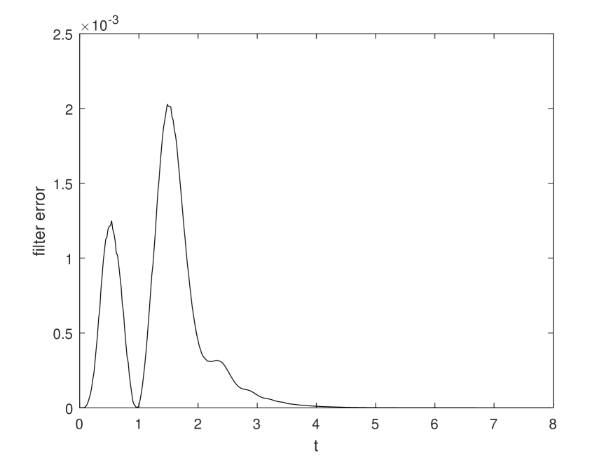
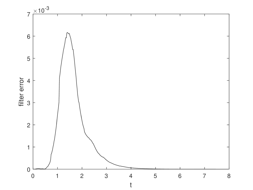
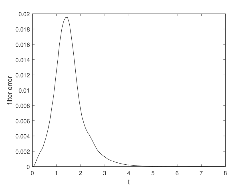
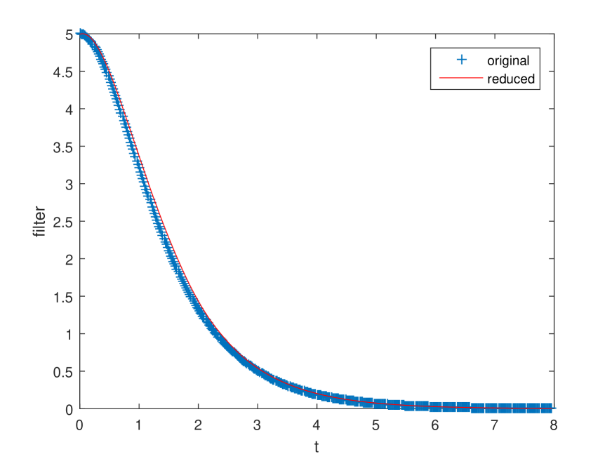
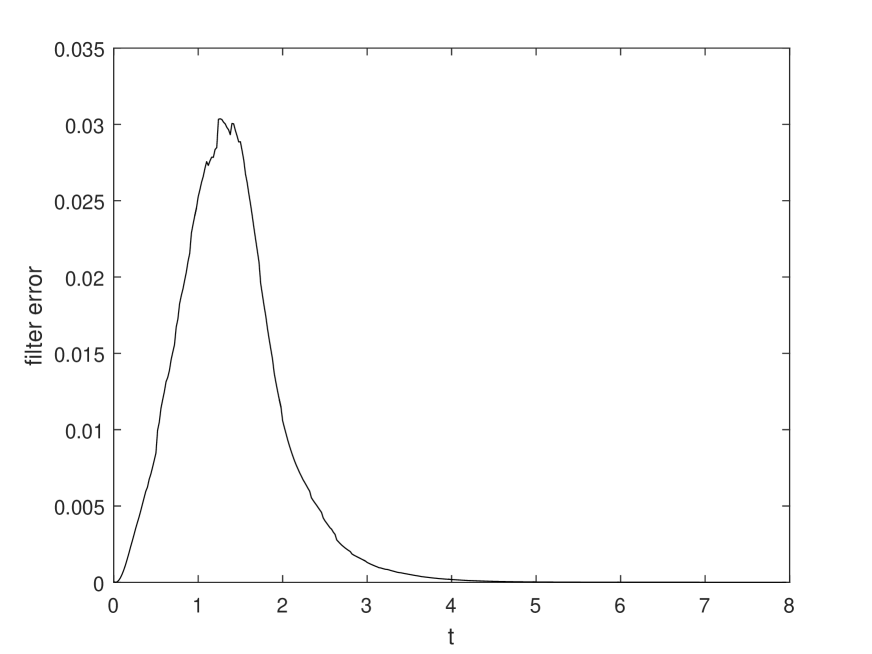
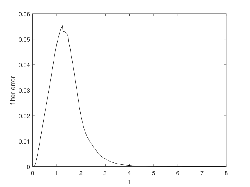
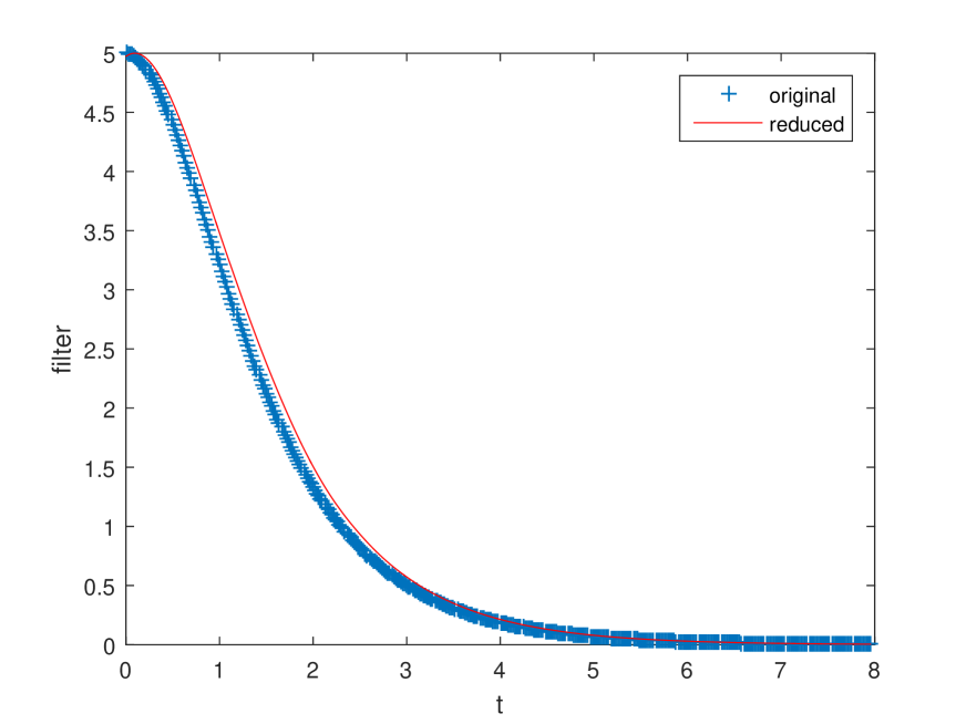
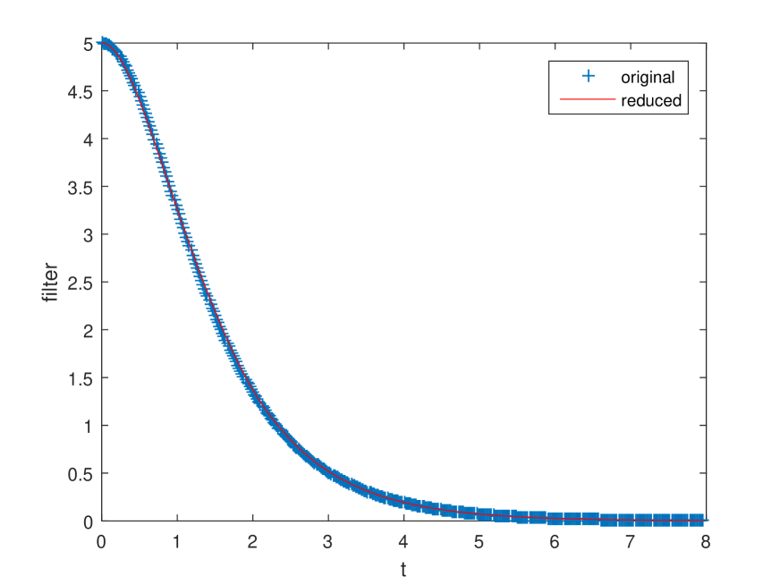
As seen in Figure 1 and Figure 2, it is clear that if the initial values of the original slow component and the reduced system are the same, the larger ε𝜀\varepsilon is, the larger the fluctuation of the filtering error is. From Figure 3 to Figure 6 it is found that if the difference for the initial values of the original slow component and the reduced system becomes larger, the fluctuation of the filtering error is larger.
Refer to caption

(a)

Refer to caption

(b)

Figure 1. (a) The original filter πtεsubscriptsuperscript𝜋𝜀𝑡\pi^{\varepsilon}_{t} (‘+’ curves) versus the reduced filter π~tεsuperscriptsubscript~𝜋𝑡𝜀\tilde{\pi}_{t}^{\varepsilon} (red curves): Initial value xε(0)=1superscript𝑥𝜀01x^{\varepsilon}(0)=1,  yε(0)=1superscript𝑦𝜀01y^{\varepsilon}(0)=1,   x~ε(0)=1superscript~𝑥𝜀01\tilde{x}^{\varepsilon}(0)=1ε=0.01𝜀0.01\varepsilon=0.01; (b) The mean-square error 𝔼|πtε(ϕ)π~tε(ϕ)|2𝔼superscriptsubscriptsuperscript𝜋𝜀𝑡italic-ϕsuperscriptsubscript~𝜋𝑡𝜀italic-ϕ2{\mathbb{E}}|\pi^{\varepsilon}_{t}(\phi)-\tilde{\pi}_{t}^{\varepsilon}(\phi)|^{2}.

Refer to caption

(c)

Refer to caption

(d)

Figure 2. (c) The original filter πtεsubscriptsuperscript𝜋𝜀𝑡\pi^{\varepsilon}_{t} (‘+’ curves) versus the reduced filter π~tεsuperscriptsubscript~𝜋𝑡𝜀\tilde{\pi}_{t}^{\varepsilon} (red curves): Initial value xε(0)=1superscript𝑥𝜀01x^{\varepsilon}(0)=1,  yε(0)=1superscript𝑦𝜀01y^{\varepsilon}(0)=1,   x~ε(0)=1superscript~𝑥𝜀01\tilde{x}^{\varepsilon}(0)=1ε=0.1𝜀0.1\varepsilon=0.1; (d) The mean-square error 𝔼|πtε(ϕ)π~tε(ϕ)|2𝔼superscriptsubscriptsuperscript𝜋𝜀𝑡italic-ϕsuperscriptsubscript~𝜋𝑡𝜀italic-ϕ2{\mathbb{E}}|\pi^{\varepsilon}_{t}(\phi)-\tilde{\pi}_{t}^{\varepsilon}(\phi)|^{2}.

Refer to caption

(e)

Refer to caption

(f)

Figure 3. (e) The original filter πtεsubscriptsuperscript𝜋𝜀𝑡\pi^{\varepsilon}_{t} (‘+’ curves) versus the reduced filter π~tεsuperscriptsubscript~𝜋𝑡𝜀\tilde{\pi}_{t}^{\varepsilon} (red curves): Initial value xε(0)=1superscript𝑥𝜀01x^{\varepsilon}(0)=1,  yε(0)=1superscript𝑦𝜀01y^{\varepsilon}(0)=1,   x~ε(0)=0.95superscript~𝑥𝜀00.95\tilde{x}^{\varepsilon}(0)=0.95ε=0.01𝜀0.01\varepsilon=0.01; (f) The mean-square error 𝔼|πtε(ϕ)π~tε(ϕ)|2𝔼superscriptsubscriptsuperscript𝜋𝜀𝑡italic-ϕsuperscriptsubscript~𝜋𝑡𝜀italic-ϕ2{\mathbb{E}}|\pi^{\varepsilon}_{t}(\phi)-\tilde{\pi}_{t}^{\varepsilon}(\phi)|^{2}.

Refer to caption

(g)

Refer to caption

(h)

Figure 4. (g) The original filter πtεsubscriptsuperscript𝜋𝜀𝑡\pi^{\varepsilon}_{t} (‘+’ curves) versus the reduced filter π~tεsuperscriptsubscript~𝜋𝑡𝜀\tilde{\pi}_{t}^{\varepsilon} (red curves): Initial value xε(0)=1superscript𝑥𝜀01x^{\varepsilon}(0)=1,  yε(0)=1superscript𝑦𝜀01y^{\varepsilon}(0)=1,   x~ε(0)=0.95superscript~𝑥𝜀00.95\tilde{x}^{\varepsilon}(0)=0.95ε=0.1𝜀0.1\varepsilon=0.1; (h) The mean-square error 𝔼|πtε(ϕ)π~tε(ϕ)|2𝔼superscriptsubscriptsuperscript𝜋𝜀𝑡italic-ϕsuperscriptsubscript~𝜋𝑡𝜀italic-ϕ2{\mathbb{E}}|\pi^{\varepsilon}_{t}(\phi)-\tilde{\pi}_{t}^{\varepsilon}(\phi)|^{2}.

Refer to caption

(i)

Refer to caption

(j)

Figure 5. (i) The original filter πtεsubscriptsuperscript𝜋𝜀𝑡\pi^{\varepsilon}_{t} (‘+’ curves) versus the reduced filter π~tεsuperscriptsubscript~𝜋𝑡𝜀\tilde{\pi}_{t}^{\varepsilon} (red curves): Initial value xε(0)=1superscript𝑥𝜀01x^{\varepsilon}(0)=1,  yε(0)=1superscript𝑦𝜀01y^{\varepsilon}(0)=1,   x~ε(0)=0.9superscript~𝑥𝜀00.9\tilde{x}^{\varepsilon}(0)=0.9ε=0.01𝜀0.01\varepsilon=0.01; (j) The mean-square error 𝔼|πtε(ϕ)π~tε(ϕ)|2𝔼superscriptsubscriptsuperscript𝜋𝜀𝑡italic-ϕsuperscriptsubscript~𝜋𝑡𝜀italic-ϕ2{\mathbb{E}}|\pi^{\varepsilon}_{t}(\phi)-\tilde{\pi}_{t}^{\varepsilon}(\phi)|^{2}.

Refer to caption

(k)

Refer to caption

(l)

Figure 6. (k) The original filter πtεsubscriptsuperscript𝜋𝜀𝑡\pi^{\varepsilon}_{t} (‘+’ curves) versus the reduced filter π~tεsuperscriptsubscript~𝜋𝑡𝜀\tilde{\pi}_{t}^{\varepsilon} (red curves): Initial value xε(0)=1superscript𝑥𝜀01x^{\varepsilon}(0)=1,  yε(0)=1superscript𝑦𝜀01y^{\varepsilon}(0)=1,   x~ε(0)=0.9superscript~𝑥𝜀00.9\tilde{x}^{\varepsilon}(0)=0.9ε=0.1𝜀0.1\varepsilon=0.1; (l) The mean-square error 𝔼|πtε(ϕ)π~tε(ϕ)|2𝔼superscriptsubscriptsuperscript𝜋𝜀𝑡italic-ϕsuperscriptsubscript~𝜋𝑡𝜀italic-ϕ2{\mathbb{E}}|\pi^{\varepsilon}_{t}(\phi)-\tilde{\pi}_{t}^{\varepsilon}(\phi)|^{2}.

6. Conclusion

In this paper, we first obtain the low dimensional reduction of a slow-fast data assimilation system via an invariant slow manifold. Then we show that the low dimensional filter on the slow manifold approximates the original filter. Moreover, by an example we illustrate this approximate filter numerically.


Acknowledgements. We would like to thank Dr. Xinyong Zhang (Tsinghua University, China) and Dr. Jian Ren (Zhengzhou University of Light Industry, China) for helpful discussions and comments.

References

  • [1] L. Arnold, Random Dynamical Systems, Springer, Berlin, 1998.
  • [2] A. Bain and D. Crisan, Fundamentals of Stochastic Filtering, Springer, Berlin, 2009.
  • [3] J. Duan, An Introduction to Stochastic Dynamics. Cambridge University Press, New York, 2015.
  • [4] S. N. Ethier and T. G. Kurtz, Markov processes: Characterization and convergence. John Wiley & Sons, 1986.
  • [5] H. Fu, X. Liu and J. Duan, Slow manifolds for multi-time-scale stochastic evolutionary systems, Comm. Math. Sci., 11(2013), 141-162.
  • [6] T. Higuchi, On the resampling scheme in the filtering procedure of the Kitagawa Monte Carlo Filter, Japan, 1995.
  • [7] P. Imkeller, N. S. Namachchivaya, N. Perkowski and H. C. Yeong, Dimensional reduction in nonlinear filtering: a homogenization approach, The Annals of Applied Probability, 23(2013), 2290-2326.
  • [8] J. H. Park, N. S. Namachchivaya and H. C. Yeong, Particle filters in a multiscale environment: Homogenized hybrid particle filter, J. Appl. Mech., 78(2011), 1-10.
  • [9] J. H. Park, R. B. Sowers and N. S. Namachchivaya, Dimensional reductionin nonlinear filtering, Nonlinearity, 23(2010), 305-324.
  • [10] J. H. Park, B. Rozovskii and R. B. Sowers, Efficient nonlinear filtering of a singularly perturbed stochastic hybrid system, LMS Journal of Computation and Mathematics, 14(2011), 254-270.
  • [11] M. Turcotte, J. Garcia-Ojalvo, and G. M. Süel, A Genetic Timer through Noise-Induced Stabilization of an Unstable State, Proceedings of the National Academy of Sciences of the United States of America, 41(2008), 15732-7.
  • [12] R. Z. Khasminskii and G.Yin, On transition densities of singularly perturbed diffusions with fast and slow components, SIAM J. APPL. MATH., 56(1996), 1794-1819.
  • [13] F. Wu, T. Tian, J. B. Rawling and George Yin, Approximate method for stochastic chemical kinetics with two-time scales by chemical Langevin equations, Journal of Chemical Physics, 144(2016), 174112.
  • [14] W. Wang and A. J. Roberts, Slow manifold and averaging for slow-fast stochastic differential system, J. Math. Anal. Appl, 398(2013), 822-839.
  • [15] Y. Kabanov and S. Pergamenshchikov, Two-scale stochastic systems: asymptotic analysis and control, Springer-Verlag, Berlin, 2003.
  • [16] G. Evensen, Data Assimilation:The Ensemble Kalman Filter, Springer-Verlag, Berlin, 2009.
  • [17] B. L. Rozovskii, Stochastic Evolution System: Linear Theory and Application to nonlinear Filtering, Springer, New York, 1990.
  • [18] Z. Schuss, Nonlinear Filtering and Optimal Phase Tracking, Springer, New York, 2012.
  • [19] E. Pardoux, Stochastics-An International Journal of Probability and Stochastic Processes, Stochastics-An International Journal of Probability and Stochastic Processes, 3(1979), 127-167.
  • [20] B. Schmalfuß and R. Schneider, Invariant manifolds for random dynamical systems with slow and fast variables, J. Dyna. Diff. Equa., 20(2008), 133-164.
  • [21] G. A. Pavliotis and A. M. Stuart, Multiscale methods: averaging and homogenization, Springer Science+Business Media, New York, 2008.
  • [22] S. Albeverio, B. Rüdiger and J. Wu, Invariant measures and symmetry property of Lévy type operators, Potential Analysis, 13(2000), 147-168.
  • [23] S. Albeverio, Z. Brzeźniak and J. Wu, Existence of global solutions and invariant measures for stochastic differential equations driven by Poisson type noise with non-Lipschitz coefficients, Journal of Mathematical Analysis and Applications, 371(2010), 309-322.