Geometric integrators and the Hamiltonian Monte Carlo method–References

Geometric integrators and the Hamiltonian Monte Carlo method

1 Introduction

This paper surveys the relations between numerical integration and the Hamiltonian (or Hybrid) Monte Carlo Method (HMC), an important and widely used Markov Chain Monte Carlo algorithm (?) for sampling from probability distributions. It is written for a general audience and requires no background on numerical algorithms for solving differential equations. We hope that it will be useful to mathematicians, statisticians and scientists, especially because the efficiency of HMC is largely dependent on the performance of the numerical integrator used in the algorithm.

Named one of the top ten algorithms of the twentieth century (?), MCMC originated in statistical mechanics (?, ?, ?, ?, ?, ?) and is now a cornerstone in statistics (?, ?, ?, ?); in fact Bayesian approaches only became widespread once MCMC made it possible to sample from completely arbitrary distributions. In conjunction with Bayesian methodologies, MCMC has enabled applications of statistical inference to biostatistics (?), population modelling (?), reliability/risk assessment/uncertainty quantification (?), machine learning (?), inverse problems (?), data assimilation (?, ?), pattern recognition (?, ?), artificial intelligence (?), and probabilistic robots (?). In these applications, MCMC is used to evaluate the expected values necessary for Bayesian statistical inference, in situations where other methods like numerical quadrature, Laplace approximation, and Monte Carlo importance sampling are impractical or inaccurate. Additionally, MCMC is used as a tool to set the invariant distribution of numerical methods for first and second-order Langevin stochastic differential equations (?, ?, ?, ?, ?, ?, ?, ?, ?, ?) and stochastic partial differential equations (?, ?). Even though MCMC algorithms are often straightforward to program, there are numerous user-friendly, general-purpose software packages available to carry out statistical analysis including BUGS (?, ?, ?), STAN (?), MCMCPack (?), MCMCglmm (?) and PyMC (?).

HMC itself was invented in 1987 (?) to study lattice models of quantum field theory, and about a decade later popularized in data science (?, ?). A simple introduction to this algorithm may be found in (?). A key feature of HMC is that it offers the possibility of generating proposal moves that, while being far away from the current state of the Markov chain, may be accepted with high probability, thus avoiding random walk behaviour and reducing the correlation between samples. Such a possibility exists because proposals are generated by numerically integrating a system of Hamiltonian differential equations. The distance between the proposal and the current state may in principle be large if the differential equations are integrated over a suitably long time interval; the acceptance probability of the proposals may be made arbitrarily close to $100\%$ by carrying out the integration with sufficient accuracy. Of particular significance for us is the fact that HMC requires that the numerical integration be performed with a volume-preserving, reversible method.

Since the computational cost of HMC mainly lies in the numerical integrations, it is of much interest to perform these as efficiently as possible. At present, the well-known velocity Verlet algorithm is the method of choice, but, as it will be apparent, Verlet may not be the most efficient integrator one could use. What does it take to design a good integrator for HMC? A key point of this paper is that, due to the specificities of the situation, a number of concepts traditionally used to analyze numerical integrators (including the notions of order of consistency/converengence, error constants, and others) are of limited value in our context. On the one hand and as we have already mentioned, HMC requires methods that have the geometric properties of being volume-preserving and reversible and this limits the number of integrators that may be applied. It is fortunate that, in the last twenty-five years, the literature on the numerical solution of differential equations has given much attention to the construction of integrators with relevant geometric properties, to the point that geometric integration (a term introduced in (?)) is by now a well-established subfield of numerical analysis (?). On the other hand, the properties of preservation of volume and reversibility have important quantitative implications on the integration error (Theorem 6.3), which in turn have an impact on the acceptance rate of proposals. As a consequence, it turns out that, for HMC purposes, the order of the integrator is effectively twice its nominal order; for instance the Verlet algorithm behaves, within HMC, as a fourth order integrator. In addition, in HMC, integrators are likely to be operated with large values of the step size, with the implication that analyses that are only valid in the limit of vanishing step size may not be very informative. One has rather to turn to studying the performance of the integrator in well-chosen model problems.

Sections 2–5 provide the necessary background on differential equations, numerical methods, geometric integration and Monte Carlo methods respectively. The heart of the paper is in Section 6. Among the topics considered there, we mention the investigation of the impact on the energy error of the properties of preservation of volume and reversibility (Theorem 6.3) and a detailed study of the behaviour of the integrators in the Gaussian model. Also presented in Section 6 is the construction of integrators more efficient than the Verlet algorithm. Sections 7 and 8 consider, in two different scenarios, the behaviour of HMC as the dimensionality of the target distribution increases. Section 7, based on (?) studies the model problem where the target is a product of many independent, identical copies. The case where the target arises from discretization of an infinite-dimensional distribution is addressed in Section 8; our treatment, while related to the material in (?), has some novel features because we have avoided the functional analytic language employed in that reference. The final Section 9 contains supplementary material.

2 Differential equations and their flows

In this section we introduce some notation and review background material on differential equations, with special emphasis on the Hamiltonian and reversible systems at the basis of HMC algorithms. The section ends with a description of the Lie bracket which appears in the analysis of the integrators to be used later.

2.1 Preliminaries

We are concerned with autonomous systems of differential equations in ${\mathbb{R}}^{D}$

$$\frac{d}{dt}x=f(x);$$ (1)

the function (vector field) $f$ is assumed throughout to be defined in the whole of ${\mathbb{R}}^{D}$ and to be sufficiently smooth. An important role is played by the particular case

$$\frac{d}{dt}q=M^{-1}p,\qquad\frac{d}{dt}p=F(q),$$ (2)

where $x=(q,p)\in{\mathbb{R}}^{D}$, $D=2d$, $q\in{\mathbb{R}}^{d}$, $p\in{\mathbb{R}}^{d}$ and $M$ is a constant, invertible matrix, so that $f=(M^{-1}p,F(q))$. By eliminating $p$, (2) is seen to be equivalent to

$$M\frac{d^{2}}{dt^{2}}q=F(q);$$

this is not the most general autonomous system of second order differential equations in ${\mathbb{R}}^{d}$ because the derivative $(d/dt)q$ does not appear in the right-hand side. When the forces depend only on the positions, Newton’s second law for a mechanical system gives rise to differential equations of the form (2); then $q$, $(d/dt)q$, $p$, $F$ are respectively the vectors of coordinates, velocities, momenta, and forces, and $M$ is the matrix of masses.

We denote by $\varphi_{t}$ the $t$-flow of the system (1) under consideration. By definition, for fixed real $t$, $\varphi_{t}:{\mathbb{R}}^{D}\to{\mathbb{R}}^{D}$ is the map that associates with each $\alpha\in{\mathbb{R}}^{D}$ the value at time $t$ of the solution of (1) that at the initial time 0 takes the initial value $\alpha$.

Example 2.1

As a very simple but important example, we consider the standard harmonic oscillator, the system in ${\mathbb{R}}^{2}$ of the special form (2) given by

$$\frac{dq}{dt}=p,\qquad\frac{dp}{dt}=-q.$$ (3)

For future reference, we note that, with matrix notation, the solutions satisfy

$$\left[\begin{matrix}q(t)\\ p(t)\end{matrix}\right]=M_{t}\left[\begin{matrix}q(0)\\ p(0)\end{matrix}\right],\qquad M_{t}=\left[\begin{matrix}\phantom{-}\cos t&\sin t\\ -\sin t&\cos t\end{matrix}\right].$$ (4)

Thus the flow has the expression

$$\varphi_{t}(\xi,\>\eta)=(\xi\cos t+\eta\sin t,\>-\xi\sin t+\eta\cos t).$$ (5)

When $\alpha=(\xi,\eta)\in{\mathbb{R}}^{2}$ is fixed and $t$ varies, the right-hand side of (5) yields the solution that at $t=0$ takes the initial value $(\xi,\eta)$. The notation $\varphi_{t}(\xi,\>\eta)$ emphasizes that, in the flow, it is the parameter $t$ that is seen as fixed, while $(\xi,\eta)\in{\mathbb{R}}^{2}$ is regarded as a variable. Geometrically, $\varphi_{t}$ is the clockwise rotation of angle $t$ around the origin of the $(q,p)$-plane.

For a given system (1), it is well possible that for some choices of $\alpha$ and $t$, the vector $\varphi_{t}(\alpha)\in{\mathbb{R}}^{D}$ is not defined; this will happen if $t$ is outside the interval in which the solution of (1) with initial value $\alpha$ exists. For simplicity in the statements, we shall assume hereafter that $\varphi_{t}(\alpha)$ is always defined.

Flows possess the group property: $\varphi_{0}$ is the indentity map in ${\mathbb{R}}^{D}$ and, for arbitrary real $s$ and $t$,

$$\varphi_{t}\circ\varphi_{s}=\varphi_{s+t}.$$ (6)

In particular, for each $t$,

$$(\varphi_{t})^{-1}=\varphi_{-t},$$ (7)

i.e.  $\varphi_{-t}$ is the inverse of the map $\varphi_{t}$. For the harmonic oscillator example, the group property simply states that a rotation of angle $s$ followed by a rotation of angle $t$ has the same effect as a rotation of angle $s+t$.

2.2 Hamiltonian systems

The Hamiltonian formalism (?, ?) is essential to understand HMC algorithms.

2.2.1 Hamiltonian vector fields

Assume that the dimension $D$ of (1) is even, $D=2d$, and write $x=(q,p)$ with $q,p\in{\mathbb{R}}^{d}$. Then the system (1) is said to be Hamiltonian if there is a function $H:{\mathbb{R}}^{2d}\rightarrow{\mathbb{R}}$ such that, for $i=1,\dots,d$, the scalar components $f^{i}$ of $f$ are given by

$$f^{i}(q,p)=+\frac{\partial H}{\partial q^{i}}(q,p),\qquad f^{d+i}(q,p)=-\frac{\partial H}{\partial p^{i}}(q,p).$$

Thus, the system is

$$\frac{dq^{i}}{dt}=+\frac{\partial H}{\partial q^{i}}(q,p),\qquad\frac{dp^{i}}{dt}=-\frac{\partial H}{\partial p^{i}}(q,p),$$

or, in vector notation (?),

$$\frac{d}{dt}\left[\begin{matrix}q\\ p\end{matrix}\right]=J^{-1}\nabla H(q,p),$$ (8)

where

$$\nabla H=\left[\frac{\partial H}{\partial q^{1}},\dots,\frac{\partial H}{\partial q^{d}},\frac{\partial H}{\partial p^{1}},\dots,\frac{\partial H}{\partial p^{d}}\right]^{T}$$

and

$$J=\left[\begin{matrix}0_{d\times d}&-I_{d\times d}\\ I_{d\times d}&\phantom{-}0_{d\times d}\end{matrix}\right].$$

The function $H$ is called the Hamiltonian, ${\mathbb{R}}^{2d}$ is the phase space, and $d$ is the number of degrees of freedom.

A system of the special form (2) is Hamiltonian if and only if $F=-\nabla\mathcal{U}(q)$ for a suitable real-valued function $\mathcal{U}$, i.e.

$$\frac{d}{dt}q=M^{-1}p,\qquad\frac{d}{dt}p=-\nabla\mathcal{U}(q);$$ (9)

when that is the case,

$$H(q,p)=\mathcal{T}(p)+\mathcal{U}(q),\qquad{\rm with}\qquad\mathcal{T}(p)=\frac{1}{2}p^{T}M^{-1}p.$$ (10)

In applications to mechanics, $\mathcal{T}$ and $\mathcal{U}$ are respectively the potential and kinetic energy and $H$ represents the total energy in the system. The harmonic oscillator (3) provides the simplest example; there $\mathcal{T}=(1/2)p^{2}$, $\mathcal{U}=(1/2)q^{2}$.

2.2.2 Symplecticness and preservation of oriented volume

A mapping $\Phi:{\mathbb{R}}^{2d}\rightarrow{\mathbb{R}}^{2d}$ is said to be symplectic or canonical if, at each point $(q,p)\in{\mathbb{R}}^{2d}$,

$$\Phi^{\prime}(q,p)^{T}J\Phi^{\prime}(q,p)=J$$ (11)

($\Phi^{\prime}(q,p)$ denotes the $2d\times 2d$ Jacobian matrix of $\Phi$). The (analytic) condition (11) has a geometric interpretation in terms of preservation of two-dimensional areas (?); such interpretation is not required to understand the rest of the paper.

When $d=1$, if we set $\Phi(q,p)=(q^{*},p^{*})$, the condition (11), after multiplying the matrices in the left-hand side, is seen to be equivalent to

$$\frac{\partial q^{*}}{\partial q}\frac{\partial p^{*}}{\partial p}-\frac{\partial q^{*}}{\partial p}\frac{\partial p^{*}}{\partial q}=1.$$

The left-hand side is the Jacobian determinant of $\Phi$ and therefore the transformation $\Phi$ is symplectic if and only if the mapping $(q,p)\mapsto(q^{*},p^{*})$ preserves oriented area in the $(q,p)$ plane, i.e. for any domain $D$ the oriented area of the image $\Phi(D)\subset{\mathbb{R}}^{2}$ coincides with the oriented area of $D$. For instance, for each $t$, the rotation in (5) is a symplectic transformation in ${\mathbb{R}}^{2}$.

For general $d$ the following result holds (?, Section 38):

Proposition 2.1

For a symplectic transformation the determinant of $\Phi^{\prime}$ equals 1. Therefore symplectic transformations preserve the oriented volume in ${\mathbb{R}}^{2d}$, i.e. $\Phi(D)$ and $D$ have the same oriented volume for each domain $D\subset{\mathbb{R}}^{2d}$.

For $d>1$ preservation of oriented volume is a strictly weaker property than symplecticness.

The proof of the following two results is easy using (11).

Proposition 2.2

The composition $\Phi_{1}\circ\Phi_{2}$ of two symplectic mappings is itself symplectic.

Proposition 2.3

The change of variables $(q,p)=\Phi(\bar{q},\bar{p})$ with $\Phi$ symplectic transforms the Hamiltonian system of differential equations (8) into a system for $(\bar{q},\bar{p})$ that is also Hamiltonian. Moreover, the Hamiltonian function $\bar{H}$ of the transformed system is the result of changing variables in $H$, i.e. $\bar{H}=H\circ\Phi$.

In view of the following important general result (?, Proposition 2.6.2) the symplecticness of the rotation (5) noted above is a manifestation of the Hamiltonian character of the harmonic oscillator.

Theorem 2.1

Let $D=2d$. The system (1) with flow $\varphi_{t}$ is Hamiltonian if and only if, for each real $t$, $\varphi_{t}$ is a symplectic mapping.

Thus symplecticness is a characteristic property that allows us to decide whether a differential system is Hamiltonian or otherwise in terms of its flow, without knowing the vector field (right-hand side) $f$ of the equation.

We recall that a flow preserves oriented volume if and only if the corresponding vector field $f$ is divergence-free ($\nabla\cdot f=\sum_{i}(\partial/\partial x^{i})f^{i}=0$). If $d>1$, there are divergence-free differential systems in ${\mathbb{R}}^{2d}$ that are not Hamiltonian; their flows preserve oriented volume but are not symplectic.

The behavior of the solutions of Hamiltonian problems is very different from that encountered in ‘general’ systems; some features that are ‘the rule’ in Hamiltonian systems are exceptional in non-Hamiltonian systems. Such special behaviour of Hamiltonian solutions may always be traced back to the symplecticness of the flow. As a very simple example, we consider once more the harmonic oscillator (3). The origin is a center: a neutrally stable equilibrium surrounded by periodic trajectories. Small perturbations of the right-hand side of (3) generically destroy the center; after perturbation the trajectories become spirals and the origin becomes either an asymptotically stable node (trajectories spiral in) or an unstable node (trajectories spiral out). However, if the perturbation is such that the perturbed system is also Hamiltonian, then the center will not disappear under small perturbations.

2.2.3 Preservation of energy

If $(q(t),p(t))$ is a solution of (8), then

$$\frac{d}{dt}H(q(t),p(t))=\nabla H(q(t),p(t))^{T}J^{-1}\nabla H(q(t),p(t))=0,$$

because $J^{-1}$ is skew-symmetric. Therefore we may state:

Theorem 2.2

The value of the Hamiltonian function is preserved by the flow of the corresponding Hamiltonian system, i.e. $H\circ\varphi_{t}=H$ for each real $t$.

In applications to the physical sciences, this result is usually the mathematical expression of the principle of conservation of energy. Unlike symplecticness, which is a characteristic property, conservation of energy on its own does not ensure that the underlying system is Hamiltonian. There are many examples of non-Hamiltonian systems whose solutions preserve the value of a suitable energy function.

2.2.4 Preservation of the canonical probability measure

Let $\beta$ denote a positive constant and assume that $H$ is such that

$$Z=\int_{{\mathbb{R}}^{2d}}\exp(-\beta H(q,p))\,dqdp<\infty.$$

Then we have the following result, which is a direct consequence of the fact that $\varphi_{t}$ preserves both the volume element $dqdp$ (Proposition 2.1) and the value of $\exp(-\beta H)$ (because, according to Theorem 2.2, it preserves the value of $H$).

Theorem 2.3

The probability measure $\mu$ in ${\mathbb{R}}^{2d}$ with density (with respect to the ordinary Lebesgue measure) $Z^{-1}\exp(-\beta H(q,p))$ is preserved by the flow of the Hamiltonian system (8), i.e. $\mu(\varphi_{t}(D))=\mu(D)$ for each domain $D\subset{\mathbb{R}}^{2d}$ and each real $t$.

In statistical mechanics (?, ?, ?), if (8) describes the dynamics of a physical system and $\beta$ is the inverse of the absolute temperature, then $\mu$ is the canonical measure that governs the distribution of $(q,p)$ over an ensemble of many copies of the given system when the system is in contact with a heat bath at constant temperature, i.e. $Z^{-1}\exp(-\beta H(q,p))dqdp$ represents the fraction of copies with momenta between $p$ and $p+dp$, and configuration between $q$ and $q+dq$. Note that under the canonical distribution, (local) minima of the energy $H$ correspond to (local) maxima of the probability density function, i.e. to modes of the distribution. Also, if the temperature decreases ($\beta$ increases), it is less likely to find the system at a location $(q,p)$ with high energy.

For Hamiltonian functions of the particular form in (10), we may factorize

$$\exp(-\beta H(q,p))=\exp(-\frac{1}{2}\beta\,p^{T}M^{-1}p)\times\exp(-\beta\,\mathcal{U}(q))$$

and therefore, under the canonical distribution, $q$ and $p$ are stochastically independent. The (marginal) distribution of the configuration variables $q$ has probability density function proportional to $\exp(-\beta\,\mathcal{U}(q))$. The momenta $p$ possess a Gaussian distribution with zero mean and covariance matrix equal to $M$. These distributions are associated with the names of Boltzmann, Gibbs and Maxwell. Hereafter we refer to the canonical measure as the Boltzmann-Gibbs distribution.

2.3 Reversible systems

Assume now that $S$ is a linear involution in ${\mathbb{R}}^{D}$, i.e. a linear map such that $S(S(x))=x$ for each $x$. A mapping $\Phi:{\mathbb{R}}^{D}\rightarrow{\mathbb{R}}^{D}$ is said to be reversible (with respect to $S$) if, for each $x$, $S(\Phi(x))=\Phi^{-1}(S(x))$ or, more compactly,

$$S\circ\Phi=\Phi^{-1}\circ S.$$ (12)

The following results have easy proofs.

Proposition 2.4

If $\Phi$ is $S$ reversible, then

$$\left|\det\Phi^{\prime}\big{(}S(\Phi(x))\big{)}\right|=\left|\det\Phi^{\prime}(x)\right|^{-1},$$

for each $x$.

Proposition 2.5

If $\Phi_{1}$ is $S$-reversible, then $\Phi_{1}\circ\Phi_{1}$ is $S$-reversible. If $\Phi_{1}$ and $\Phi_{2}$ are $S$-reversible, then the symmetric composition $\Phi_{1}\circ\Phi_{2}\circ\Phi_{1}$ is $S$-reversible.

Theorem 2.4

Consider the system (1) with flow $\varphi_{t}$. The following statements are equivalent:

• For each $t$, $\varphi_{t}$ is an $S$-reversible mapping.

• For each $x\in{\mathbb{R}}^{D}$, $S(f(x))=-f(S(x))$, i.e. $S\circ f=-f\circ S$.

Systems of differential equations that satisfy the conditions in the theorem are said to be reversible (with respect to $S$). Systems of the particular form (2) are reversible with respect to the momentum flip involution

$$S(q,p)=(q,-p).$$ (13)

If (2) describes a mechanical system, then (12) expresses the well-known time-reversibility of mechanics: if $(q_{in},p_{in})$ is the initial state of a system and $(q_{f},p_{f})$ the final state after $t$ units of time have elapsed, then the state $(q_{f},-p_{f})$ evolves in $t$ units of time to the state $(q_{in},-p_{in})$.

Proposition 2.6

The Hamiltonian system (8) is reversible with respect to the momentum flip involution (13) if and only if $H$ is an even function of $p$, i.e. $H(q,-p)=H(q,p)$ for all $q$ and $p$.

Figure 6.1 illustrates the reversibility of the Hamiltonian flow corresponding to a one-degree-of freedom double-well potential.

As it is the case for Hamiltonian systems, reversible reversible systems have flows with special geometric properties, not shared by ‘general’ systems (?).

2.4 The Lie bracket

If $\varphi_{t}^{(f)}$ and $\varphi_{t}^{(g)}$ denote respectively the flows of the $D$-dimensional systems

$$\frac{d}{dt}x=f(x),\qquad\frac{d}{dt}x=g(x),$$

in general $\varphi_{s}^{(g)}\circ\varphi_{t}^{(f)}\neq\varphi_{t}^{(f)}\circ\varphi_{s}^{(g)}$; in fact, a Taylor expansion shows that, as $t$, $s$ approach $0$,

$$\varphi_{s}^{(g)}\big{(}\varphi_{t}^{(f)}(x)\big{)}-\varphi_{t}^{(f)}\big{(}\varphi_{s}^{(g)}(x)\big{)}=st\,[f,g](x)+\mathcal{O}(t^{3}+s^{3}),$$

where the Lie bracket (or Lie-Jacobi bracket or commutator) $[f,g]$ of $f$ and $g$ (?, Section 39) is the mapping ${\mathbb{R}}^{D}\rightarrow{\mathbb{R}}^{D}$ that at $x\in{\mathbb{R}}^{D}$ takes the value

$$[f,g](x)=g^{\prime}(x)f(x)-f^{\prime}(x)g(x)$$ (14)

Thus the magnitude of $[f,g]$ measures the lack of commutativity of the corresponding flows. The following result holds:

Theorem 2.5

With the preceding notation, $\varphi_{s}^{(g)}\circ\varphi_{t}^{(f)}=\varphi_{t}^{(f)}\circ\varphi_{s}^{(g)}$ for arbitrary $t$ and $s$ if and only if the Lie bracket $[f,g](x)$ vanishes at each $x\in{\mathbb{R}}^{D}$. When these conditions hold, we say that $f$ and $g$ commute.

For commuting $f$ and $g$, $\varphi_{t}^{(g)}\circ\varphi_{t}^{(f)}=\varphi_{t}^{(f)}\circ\varphi_{s}^{(g)}$ provides the $t$ flow of the system

$$\frac{d}{dt}x=f(x)+g(x).$$

The Lie bracket is skew symmetric: $[f,g]=-[g,f]$ for arbitrary $f$ and $g$. In addition it satisfies the Jacobi identity,

$$[f_{1},[f_{2},f_{3}]]+[f_{2},[f_{3},f_{1}]]+[f_{3},[f_{1},f_{2}]]=0,$$

for any $f_{1}$, $f_{2}$, $f_{3}$. In this way the vector space of all vector fields together with the operation $[\cdot,\cdot]$ is a Lie algebra.

For Hamiltonian systems it is possible to work in terms of the so-called Poisson bracket of the Hamiltonian functions (?, Section 40), rather than in terms of the Lie bracket of the fields:

Theorem 2.6

If the fields $f$ and $g$ are Hamiltonian with Hamiltonian functions $H$ and $K$ respectively, i.e. $f=J^{-1}\nabla H$, $g=J^{-1}\nabla K$, then $[f,g]$ is also a Hamiltonian vector field. Moreover the Hamiltonian function of $[f,g]$ is given by $-\{H,K\}$, where $\{H,K\}$ is the Poisson bracket of the functions $H$ and $K$, defined as

$$\{H,K\}=(\nabla H)^{T}J^{-1}\nabla K.$$

For real-valued functions in ${\mathbb{R}}^{2d}$, the Poisson bracket operation is skew symmetric $\{H,K\}=-\{K,H\}$ and satisfies the Jacobi identity:

$$\{H_{1},\{H_{2},H_{3}\}\}+\{H_{2},\{H_{3},H_{1}\}\}+\{H_{3},\{H_{1},H_{2}\}\}=0.$$

Let $f$ and $g$ be reversible vector fields. Differentiation in $g(S(x))=-S(g(x))$ implies for the Jacobian that $g^{\prime}(S(x))S=-S(g^{\prime}(x))$ and it follows that $g^{\prime}(S(x))f(S(x)))=S(g^{\prime}(x)f(x))$ (no minus sign!). Then the Lie-bracket of two reversible fields is not reversible, but rather satisfies the following property.

Proposition 2.7

If two vector fields $f$ and $g$ are $S$-reversible then

$$[f,g](S(x))=S\big{(}[f,g](x)\big{)}.$$

For three $S$-reversible vector fields, the iterated commutator $[f_{1},[f_{2},f_{3}]]$ is $S$-reversible.

3 Integrators

In the sampling algorithms studied later, differential systems like (1) or (2) have to be numerically integrated. In this section we review the required material. The works (?, ?, ?) provide extensive, authoritative treatises on the subject. A more concise introduction is given by (?). We begin by recalling some basic definitions and later focus on splitting integrators and fixed $h$ stability, as both play important roles in the implementation of HMC algorithms.

3.1 Preliminaries

Each one-step numerical method or one-step integrator for (1) is described by a map $\psi_{h}:{\mathbb{R}}^{D}\to{\mathbb{R}}^{D}$ that depends on a real parameter $h$, the step size. Given the initial value $\alpha$, and a value of $h$ ($h\neq 0$), the integrator generates a numerical trajectory, $x_{0}$, $x_{1}$, $x_{2}$, …, defined by $x_{0}=\alpha$ and, iteratively,

$$x_{n+1}=\psi_{h}(x_{n}),\qquad n=0,1,2,\dots$$ (15)

To compute $x_{n+1}$ when $x_{n}$ has already been found is to perform a (time) step. For each $n$, the vector $x_{n}$ is an approximation to the value at time $t_{n}=nh$ of the solution $x(t)$ of (1) with initial condition $x(0)=\alpha$, i.e. to $\varphi_{t_{n}}(\alpha)$. Typically $h$ is positive and then the integration is forward in time $0=t_{0}<t_{1}<t_{2}<\dots$, but in some applications it may be of interest to use $h<0$ so as to get $0=t_{0}>t_{1}>t_{2}>\dots$

The simplest and best known integrator, Euler’s rule, with

$$x_{n+1}=x_{n}+hf(x_{n}),$$ (16)

corresponds to the mapping $\psi_{h}(x)=x+hf(x)$. It uses one evaluation of $f$ per step. Explicit $s$-stage Runge-Kutta formulas use $s$ evaluations of $f$ per step, $s=1,2,\dots$, and are therefore $s$ times more expensive per step than Euler’s rule; examples include Runge’s method

$$\psi_{h}(x)=x+hf\big{(}x+\frac{h}{2}f(x)\big{)}$$

(with two stages), several well-known formulas of Kutta with four stages and the formulas within the popular MATLAB function ode45. A method with $s$ stages will be competitive with Euler’s rule only if it gives more accurate approximations than Euler’s rule when this is operated with a step size $s$ times shorter, so as to equalize computational costs.

Implicit Runge-Kutta integrators are also used in practice; in them $\psi_{h}$ is defined by means of algebraic equations. For instance, the midpoint rule has

$$\psi_{h}(x)=x+hf\big{(}\frac{1}{2}(x+\psi_{h}(x))\big{)},$$

i.e.

$$x_{n+1}=x_{n}+hf\big{(}\frac{1}{2}(x_{n}+x_{n+1})\big{)}.$$ (17)

Here, computing $x_{n+1}$ when $x_{n}$ is already known requires to solve a system of algebraic equations in ${\mathbb{R}}^{D}$. There are many more useful examples of implicit Runge-Kutta methods, including the so-called Gauss methods.

Remark 3.1

Note that in the formulas displayed above $h$ and $f$ do not appear separately, but always in the combination $hf$. This clearly implies that, if, for a given method, $x_{n}$, $n=0,1,2\dots$ is a numerical trajectory with step size $h$ corresponding to the system (1), it is also a numerical trajectory with step size $\lambda h$ for the system $(d/dt)x=\lambda^{-1}f(x)$ ($\lambda\neq 0$ denotes a constant). We shall always assume that we deal with integrators having this property.

A one-step integrator is called symmetric or self-adjoint if

$$(\psi_{h})^{-1}=\psi_{-h},$$ (18)

so as to mimic the property (7) of the exact solution flow. The midpoint rule (17) provides an example. Explicit Runge-Kutta methods are never symmetric.

Multistep integrators, including the well-known Adams formulas, where the computation of $x_{n+1}$ requires the knowledge of $k\geq 2$ past values $x_{n}$, $x_{n-1}$, …, $x_{n-k+1}$, may be very efficient, but will not be considered in this paper; they have seldom been applied within sampling algorithms.

3.2 Order

Since for the exact solution, the sequence $x(0)=\alpha$, $x(t_{1})$, $x(t_{2})$,… satisfies $x(t_{n+1})=\varphi_{h}(x(t_{n}))$, $n=0,1,\dots$, rather than (15), for the numerical integrator to make sense it is necessary that $\psi_{h}$ be an approximation to $\varphi_{h}$. The integrator is said to be consistent if, at each fixed $x\in{\mathbb{R}}^{D}$, $\psi_{h}(x)-\varphi_{h}(x)=\mathcal{O}(h^{2})$ as $h\rightarrow 0$. If $\psi_{h}(x)-\varphi_{h}(x)=\mathcal{O}(h^{\nu+1})$, $\nu$ a positive integer, then the integrator is (consistent) of order $\geq\nu$. A method of order $\geq\nu$ that is not of order $\geq\nu+1$ is said to have order $\nu$. Euler’s rule (16) has order 1, the four-stage formulas of Kutta have order 4 and the midpoint rule (17) has order 2. We shall see later (Theorem 4.4) that the order of a symmetric integrator is an even integer. All integrators to be considered hereafter are assumed to be consistent.

The vector $\psi_{h}(x)-\varphi_{h}(x)$ is called the local error at $x$: it is the difference between the result of a single time-step of the numerical method starting from $x$ and the result of the application of the $h$-flow to the same point $x$. For future reference, we note that the expansion of the local error for Euler’s method is given by

$$\psi_{h}(x)-\varphi_{h}(x) = \Big{(}x+hf(x)\Big{)}-\Big{(}x+hf(x)+\frac{h^{2}}{2}f^{\prime}(x)f(x)+\mathcal{O}(h^{3})\Big{)}$$ (19)

$$= -\frac{h^{2}}{2}f^{\prime}(x)f(x)+\mathcal{O}(h^{3}).$$

In the expansion of the true solution flow we have used that $(d/dt)x=f(x)$ and $(d^{2}/dt^{2})x=f^{\prime}(x)(d/dt)x=f^{\prime}(x)f(x)$.

The local error does not give per se information on the global error at $t_{n}$, i.e. on the difference $x_{n}-x(t_{n})$. This is because $x_{n}=\psi_{h}(x_{n-1})$ while $x(t_{n})$ is the result of the application of the $h$-flow to $x(t_{n-1})$: $\psi_{h}$ and $\varphi_{h}$ are not applied to the same point. However the following result holds:

Theorem 3.1

If the (one-step) integrator is consistent of order $\nu$, then, for each fixed initial value $x_{0}=x(0)$ and $T>0$,

$$\max_{0\leq t_{n}\leq T}|x_{n}-x(t_{n})|=\mathcal{O}(h^{\nu}),\qquad h\rightarrow 0+.$$ (20)

This expresses the fact that the integrator is convergent of order $\nu$. Of course, the corresponding result holds if the integration is carried out backward in time over $-T\leq t\leq 0$.

Remark 3.2

The global errors $x_{n}-x(t_{n})$ in addition to possessing an $\mathcal{O}(h^{\nu})$ bound as above, have an asymptotic expansion in powers of $h$. For instance, if we restrict the attention to the leading $h^{\nu}$ term in the expansion, we have

$$x_{n}-x(t_{n})=h^{\nu}a(x(0),t_{n})+h^{\nu}r(x(0),t_{n};h),$$

where the function $a$ is independent of $h$ and, for each fixed initial value $x(0)$, $\max_{0\leq t\leq T}|r(x(0),t,h)|$ tends to $0$ as $h\rightarrow 0+$. Thus, for $h$ sufficiently small, the global error is approximately equal to $h^{\nu}a(x(0),t_{n})$: halving $h$ divides the error by a factor $2^{\nu}$.

Remark 3.3

In the description above, the step points $t_{n}$ are uniformly spaced. General purpose software uses variable time steps: $t_{n+1}=t_{n}+h_{n}$ where $h_{n}$ changes with $n$. For each $n$, the value of $h_{n}$ is chosen by the algorithm to ensure that the local error at $x_{n}$ is below a user-prescribed tolerance. Since, for reasons to be explained in Section 4, HMC integrations are carried out with constant step size, we shall not concern ourselves with variable step sizes.

3.3 Splitting methods

Euler’s method and the other integrators mentioned above may be applied to any given system (1). Other techniques only make sense for particular classes of systems and cannot therefore be incorporated into general purpose software; however they have gained much popularity in the last decades due, among other things, to their role in geometric integration (see Section 4). Of special importance to us is the class of splitting integrators that we consider next. The monograph (?) is a very good source of information.

3.3.1 The Lie-Trotter formula

Splitting methods are applicable to cases where the right hand-side of (1) may be split into two parts

$$\frac{d}{dt}x=f(x)=f^{(A)}(x)+f^{(B)}(x),$$ (21)

in such a way that the flows $\varphi_{t}^{(A)}$ and $\varphi_{t}^{(B)}$ of the split systems

$$\frac{d}{dt}x=f^{(A)}(x),\qquad\frac{d}{dt}x=f^{(B)}(x),$$ (22)

are available analytically. To avoid trivial cases, we shall hereafter assume that the Lie bracket $[f^{(A)},f^{(B)}]$ does not vanish identically, because otherwise Theorem 2.5 shows that (21) may also be solved analytically without resorting to numerical approximations.

Systems of the particular form (2) provide an important example. When they are split by taking

$$(A):\qquad\frac{d}{dt}q=M^{-1}p,\qquad\frac{d}{dt}p=0.$$ (23)

and

$$(B):\qquad\frac{d}{dt}q=0,\qquad\frac{d}{dt}p=F(q),$$ (24)

the flows are explicitly given by

$$\varphi_{t}^{(A)}(q,p)=(q+tM^{-1}p,p)$$

and

$$\varphi_{t}^{(B)}(q,p)=(q,p+tF(q)).$$

In molecular dynamics (?) these mappings are respectively called a drift ($q$ advances with constant speed and the momentum $p$ remains constant) and a kick (the system stays in its current configuration, and the momentum is incremented by the action of the force). A direct computation of the Lie bracket shows that, except in the trivial case where $F$ vanishes identically, the vector fields in (23)–(24) do not commute.

A simple Taylor expansion proves that the Lie-Trotter formula

$$\psi_{h}=\varphi_{h}^{(B)}\circ\varphi_{h}^{(A)}$$ (25)

defines a first-order integrator for (21):

$$\psi_{h}(x)-\varphi_{h}(x)=\frac{h^{2}}{2}[f^{(A)},f^{(B)}](x)+\mathcal{O}(h^{3}).$$ (26)

(Observe that, not unexpectedly, the coefficient of the leading power of $h$ is proportional to the Lie bracket.) While $f^{(A)}$ and $f^{(B)}$ contribute simultaneously to the change of $x$ in (21), they do so successively in the Lie-Trotter integrator. By swapping the roles of $A$ and $B$, we have the alternative integrator

$$\psi_{h}=\varphi_{h}^{(A)}\circ\varphi_{h}^{(B)}.$$

3.3.2 Strang’s formula

The most popular splitting integrator for (21) corresponds to Strang’s formula (?)

$$\psi_{h}=\varphi_{(1/2)h}^{(B)}\circ\varphi_{h}^{(A)}\circ\varphi_{(1/2)h}^{(B)}$$ (27)

and, as a Taylor expansion shows, has second order accuracy, $\psi_{h}(x)-\varphi_{h}(x)=\mathcal{O}(h^{2})$ as $h\rightarrow 0$. More precisely,

$$\psi_{h}(x)-\varphi_{h}(x) = \frac{h^{3}}{12}[f^{(A)},[f^{(A)},f^{(B)}]](x)$$ (28)

$$\qquad+\frac{h^{3}}{24}[f^{(B)},[f^{(A)},f^{(B)}]](x)+\mathcal{O}(h^{4}),$$

so that the leading term of the local error is a linear combination of two so-called iterated Lie brackets.

When applied to the particular case (2), the formula (27) yields the well-known velocity Verlet integrator, the method of choice in molecular dynamics; the step $n\rightarrow n+1$ comprises two kicks of duration $h/2$ separated by a drift of duration $h$:

$$p_{n+1/2} = p_{n}+\frac{h}{2}F(q_{n}),$$

$$q_{n+1} = q_{n}+hM^{-1}p_{n+1/2},$$

$$p_{n+1} = p_{n+1/2}+\frac{h}{2}F(q_{n+1}).$$

The evaluations of $F$ represent the bulk of the computational cost of the algorithm. The value $F(q_{n+1})$ to be used in the first kick of the next step, $n+1\rightarrow n+2$, is the same used in the second kick of the current step. In this way, while the very first step requires two evaluations of $F$, subsequent steps only need one.

When $N$ steps of the method (27) are taken, the map that advances the numerical solution from $x_{0}$ to $x_{N}$, i.e.

$$\psi_{h}^{N}=\overbrace{\Big{(}\varphi_{(1/2)h}^{(B)}\circ\varphi_{h}^{(A)}\circ\varphi_{(1/2)h}^{(B)}\Big{)}\circ\cdots\circ\Big{(}\varphi_{(1/2)h}^{(B)}\circ\varphi_{h}^{(A)}\circ\varphi_{(1/2)h}^{(B)}\Big{)}}^{N\>\rm times}$$

may be rewritten with the help of the group property (6) in the leapfrog form

$$\psi_{h}^{N}=\varphi_{(1/2)h}^{(B)}\circ\overbrace{\Big{(}\varphi_{h}^{(A)}\circ\varphi_{h}^{(B)}\Big{)}\circ\cdots\circ\Big{(}\varphi_{h}^{(A)}\circ\varphi_{h}^{(B)}\Big{)}}^{N-1\>\rm times}\circ\,\varphi_{h}^{(A)}\circ\varphi_{(1/2)h}^{(B)};$$

now the right hand-side only uses $N+1$ times the flow $\varphi_{t}^{(B)}$. In the particular case (23)–(24), the combination $\varphi_{h}^{(A)}\circ\varphi_{h}^{(B)}$ corresponds to the following formulas to advance the numerical solution, $n=1,\dots,N-1$,

$$p_{n+1/2} = p_{n-1/2}+hF(q_{n}),$$

$$q_{n+1} = q_{n}+hM^{-1}p_{n+1/2};$$

$p$ jumps over $q$ and then $q$ jumps over $p$ as children playing leapfrog. The leapfrog implementation makes apparent the truth of an earlier observation: $N$ steps of the velocity Verlet integrator may be implemented with $N+1$ evaluations of $F$.

Strang’s method is symmetric:

$$(\psi_{h})^{-1} =\big{(}\varphi_{(1/2)h}^{(B)}\big{)}^{-1}\!\circ\big{(}\varphi_{h}^{(A)}\big{)}^{-1}\!\circ\big{(}\varphi_{(1/2)h}^{(B)}\big{)}^{-1}$$

$$=\varphi_{-(1/2)h}^{(B)}\circ\varphi_{-h}^{(A)}\circ\varphi_{-(1/2)h}^{(B)}$$

$$=\psi_{-h}.$$

It is clear that the symmetry is a consequence of the palindromic structure of (27) i.e. the formula reads the same from left to right as from right to left.

The roles of $A$ and $B$ in (27), may be interchanged:

$$\psi_{h}=\varphi_{(1/2)h}^{(A)}\circ\varphi_{h}^{(B)}\circ\varphi_{(1/2)h}^{(A)}.$$ (29)

For (23)–(24) one then obtains the position Verlet integrator: one step comprises two drifts of duration $h/2$ and one kick of duration $h$.

3.3.3 Splitting formulas with more stages

It is of course possible to use splitting formulas more sophisticated than Strang’s. For instance, for any choice of the real parameter $b$, we may consider the integrator

$$\psi_{h}=\varphi_{bh}^{(B)}\circ\varphi_{(1/2)h}^{(A)}\circ\varphi_{(1-2b)h}^{(B)}\circ\varphi_{(1/2)h}^{(A)}\circ\varphi_{bh}^{(B)},$$ (30)

where we observe that, in one step, the $A$ and $B$ flows of the systems (22) act for a total duration of $h$ units of time each to ensure consistency. Due to its palindromic structure, this integrator is symmetric and from Theorem 4.4 its order is at least two. It turns out that the order is exactly two for all choices of $b$ (?). The order of splitting integrators is discussed later in relation with the concept of modified equations.

Even though three $B$ flows and two $A$ flows feature in (30), $N$ steps of the integrator only require the computation of $2N+1$ $B$ flows and $2N$ $A$ flows; this is seen by combining flows as we did above for the Strang case. We say that (30) is a palindromic two stage integrator. The method (30) may be denoted by

$$\big{(}b,1/2,(1-2b),1/2,b\big{)}.$$ (31)

Similarly, one may consider the two-parameter family of palindromic three-stage splittings

$$\big{(}b,a,1/2-b,1-2a,1/2-b,a,b\big{)}.$$ (32)

A full description of this family is given by (?); this reference suggests parameter choices for various applications. There is a unique choice of $a$ and $b$ resulting in a fourth-order method often associated with Yoshida’s name (?); for all other choices, the order is $\nu=2$.

The family of palindromic $s$-stage splitting formulas is given by

$$\big{(}b_{1},a_{1},b_{2},a_{2},\dots,a_{s^{\prime}},b_{s^{\prime}+1},a_{s^{\prime}},\dots,a_{2},b_{2},a_{1},b_{1}\big{)},$$ (33)

if $s=2s^{\prime}$ is even, and by

$$\big{(}b_{1},a_{1},b_{2},a_{2},\dots,b_{s^{\prime}},a_{s^{\prime}},b_{s^{\prime}},\dots,a_{2},b_{2},a_{1},b_{1}\big{)},$$ (34)

if $s=2s^{\prime}-1$. After imposing the consistency requirement that at each step the $A$ and $B$ flows act during $h$ units of time each, the family has $s-1$ parameters left. By taking $s$ sufficiently high it is possible to achieve any desired order (?, Section 13.1). Clearly, increasing the number of stages does not lead to integrators with a more complicated implementation; regardless of the value of $s$ numerical integrations just consist of a sequence of flows of the split systems.

It is not necessary to add that to each of the integrators just described there corresponds a second integrator found by swapping the roles of the systems $A$ and $B$, just as (29) corresponds to (27).

So far our attention has focused on palindromic formulas as these are important later in connection with the property of reversibility (Theorem 4.2). It is also possible to consider splittings of the form:

$$\psi_{h}=\varphi_{b_{r}h}^{(B)}\circ\varphi_{a_{r}h}^{(A)}\circ\cdots\circ\varphi_{b_{2}h}^{(B)}\circ\varphi_{a_{2}h}^{(A)}\circ\varphi_{b_{1}h}^{(B)}\circ\varphi_{a_{1}h}^{(A)},$$

that we denote as

$$\big{(}b_{r},a_{r},\dots,b_{2},a_{2},b_{1},a_{1}\big{)}.$$ (35)

($\sum_{i}a_{i}=\sum_{i}b_{i}=1$). The palindromic formulas in (33)–(34) are particular instances of this general format because it is always possible to set $a_{1}=0$ in (35).

Remark 3.4

When a splitting integrator of the general form (35) is applied to the splitting (23)–(24) of the system (2), the result coincides with the application of a so-called symplectic, explicit Runge-Kutta-Nyström (RKN) method. The properties (order, stability, etc.) of such an integrator may therefore be studied either by using techniques pertaining to splitting integrators (as done in this paper) or by employing an RKN approach. The second methodology was favoured in the early years of geometric integration (?, ?).

3.4 Fixed $h$ stability

If two numerical schemes are candidates to integrate an initial value problem for a given system (1), then the scheme that leads to smaller global errors for a given computational cost may seem more desirable (but, in the context of geometric integration, the geometric properties may play a role when choosing the integrator, see Section 4 below). Even though global errors may be bounded as in (20), in practice, it is almost always impossible, for the problem at hand, to estimate realistically the error constant implied in the $\mathcal{O}(h^{\nu})$ notation in the bound. For this reason, the literature on numerical integrators has traditionally resorted to well-chosen model problems where both the numerical and true solutions, $x_{n}$ and $x(t_{n})$, may be written down in closed form; the performance of the various integrators on the model problem may then be investigated analytically and is taken as an indication of their performance when applied to realistic problems. Note that the actual numerical solution of the model problem cannot be expected to be of real practical interest, since in that problem the true solution is available analytically.

3.4.1 One degree of freedom

For our purposes, the model problem of choice is the harmonic oscillator (3). For Runge-Kutta methods, for the splitting algorithms in Section 3.3 (and in fact for all one-step integrators of practical interest) a time-step $(q_{n+1},p_{n+1})=\psi_{h}(q_{n},p_{n})$ may be expressed as

$$\left[\begin{matrix}q_{n+1}\\ p_{n+1}\end{matrix}\right]=\tilde{M}_{h}\left[\begin{matrix}q_{n}\\ p_{n}\end{matrix}\right],\qquad\tilde{M}_{h}=\left[\begin{matrix}A_{h}&B_{h}\\ C_{h}&D_{h}\end{matrix}\right]$$ (36)

for suitable method-dependent coefficients $A_{h}$, $B_{h}$, $C_{h}$, $D_{h}$. The evolution over $n$ time-steps is then given by

$$\left[\begin{matrix}q_{n}\\ p_{n}\end{matrix}\right]=\tilde{M}_{h}^{n}\left[\begin{matrix}q_{0}\\ p_{0}\end{matrix}\right],$$ (37)

an expression to be compared with (4).

If a given $h>0$ is such that $|\tilde{M}_{h}^{n}|\rightarrow\infty$ as $n\rightarrow\infty$, the magnitude of numerical solution $(q_{n},p_{n})$ will grow unboundedly, while the true solution of course remains bounded as $t\rightarrow\infty$. Necessarily, global errors will be large for large $n$. Then the integrator is said to be unstable for that particular choice of $h$.

Example 3.1

For Euler’s rule (16) we find

$$A_{h}=D_{h}=1,\quad B_{h}=-C_{h}=h.$$

The eigenvalues of $\tilde{M}_{h}$ are $1\pm ih$ with modulus $(1+h^{2})^{1/2}$ and, therefore, for any fixed $h>0$, the powers $\tilde{M}_{h}^{n}$ grow exponentially as $n$ increases. Due to this numerical instability, Euler’s rule is completely unsuitable to integrate the harmonic oscillator, and this rules it out as a method to integrate more complicated oscillatory problems.

More precisely, in the step $n\rightarrow n+1$, the radius $r=(q^{2}+p^{2})^{1/2}$, which remains constant for the true solution, grows like

$$r_{n+1}=(1+h^{2})^{1/2}r_{n}=\left(1+\frac{h^{2}}{2}+\mathcal{O}(h^{4})\right)r_{n}$$ (38)

for the Euler solution, so that $r_{n}=(1+h^{2})^{n/2}r_{0}$. Note that, taking limits as $n\rightarrow\infty$, $h\rightarrow 0$, with fixed $nh$, we find $r_{n}\rightarrow r_{0}=r(0)=r(nh)$, as it corresponds to a convergent method.

Example 3.2

The midpoint rule (17) has

$$A_{h}=D_{h}=\frac{1-\frac{h^{2}}{4}}{1+\frac{h^{2}}{4}},\quad B_{h}=-C_{h}=\frac{h}{1+\frac{h^{2}}{4}}.$$

The characteristic equation of $\tilde{M}_{h}$ is

$$\lambda^{2}-2A_{h}\lambda+1$$ (39)

and therefore the product of the eigenvalues is 1. For $h\neq 0$, $|A_{h}|<1$ and the matrix has a pair of complex conjugate eigenvalues of unit modulus. Then the powers $\tilde{M}_{h}^{n}$ remain bounded as $n$ increases and the method is stable for any $h$.

Example 3.3

Let us next consider Strang’s splitting (27), applied with the splitting (23)–(24), which yields the velocity Verlet algorithm. This has

$$A_{h}=D_{h}=1-h^{2}/2,\quad B_{h}=h,\quad C_{h}=-h+h^{3}/4;$$

the characteristic equation is again of the form (39). For $h>2$, $A_{h}<-1$ and the eigenvalues are real and distinct, so that one of them has modulus $>1$, and therefore the powers $\tilde{M}_{h}^{n}$ grow exponentially. For $h<2$ the eigenvalues are complex of unit modulus and the powers $\tilde{M}_{h}^{n}$ remain bounded. For $h=2$, $\tilde{M}_{h}$ is a nontrivial Jordan block whose powers grow linearly (weak instability). To summarize, the integrator is unstable for $h\geq 2$ and has the stability interval $0<h<2$. Integrations with $h>2$ lead to extremely large global errors as we shall see below.

Example 3.4

For the alternative Strang formula (29), which yields the position Verlet algorithm, the coefficients are

$$A_{h}=D_{h}=1-h^{2}/2,\quad B_{h}=h-h^{3}/4,\quad C_{h}=-h.$$

The discussion is almost identical to the one in the preceding example. The stability interval is also $0<h<2$, as one may have guessed from the equal role that $q$ and $-p$ play in the harmonic oscillator (3).

$h$	$t=T_{per}$	$t=10\,T_{per}$
$T_{per}/4$	6.49e-1	2.00e0
$T_{per}/8$	1.60e-1	1.48e0
$T_{per}/16$	4.03e-2	4.00e-1
$T_{per}/32$	1.01e-2	1.01e-1

Table 3.1: Velocity Verlet integration of the harmonic oscillator. Relative errors after one or ten oscillation periods

Example 3.5

In the situation of Example 3.3, are values of $h$ below the upper limit 2 satisfactory? The answer of course depends on the accuracy required. Table 3.1 gives, for the initial condition $q=1$, $p=0$, and different stable values of $h$, the relative error in the Euclidean norm

$$\frac{|(q_{n}-q(t_{n}),p_{n}-p(t_{n}))|}{|(q(t_{n}),p(t_{n}))|}$$

at the final integration time, when the integration is carried out over an interval of length either one oscillation period (second column) or ten oscillation periods (third column). Columns are consistent with the order of convergence as in (20). The last rows reveal that the error increases linearly with $t$ (this will not be true when integrating other differential systems). In the first row the error grows more slowly than $t$: the numerical solution $(q_{n},p_{n})$ remains close to the unit circle for all values of $n$ and therefore errors cannot be substantially larger than the diameter of the circle. From the table we see that if we are interested in errors below $10\%$ over an interval of length equal to ten oscillation periods, then $h$ has to be taken below $2\pi/32\approx 0.20$, i.e. well below the upper end, $h=2$, of the stability interval. To provide an indication of the effect of using unstable values of $h$, we mention that with $h=\pi$ the error after one period is $\approx 46.4$ and after ten periods $\approx 4.68\times 10^{17}$.

Before we move to more complicated models, let us make two observations, valid for Runge-Kutta, splitting integrators and any other method of practical interest.

Remark 3.5

Because the problem is linear and rotationally invariant, the magnitude of the relative errors is independent of the initial condition $(q_{0},p_{0})\neq(0,0)$.

Remark 3.6

Replacing the model (3) with the apparently more general system

$$\frac{dq}{dt}=\omega p,\qquad\frac{dp}{dt}=-\omega q,\qquad\omega>0,$$ (40)

with oscillation period $2\pi/\omega$, does not really change things: in view of Remark 3.1 integrating (40) with step size $h$ is equivalent to integrating (3) with step size $h/\omega$. Because the length of the integration interval and the step size in Table 3.1 are given in terms of the oscillation period, the results displayed are valid for (40) for any choice of the value of $\omega$. Regardless of the initial condition, if we are interested in relative errors below $10\%$ over an interval of length $20\pi/\omega$ (equal to ten oscillation periods), then $h$ has to be taken below $2\pi/(32\omega)$. Of course, for (40), stability requires that $h<2/\omega$.

3.4.2 Several degrees of freedom. Stability restrictions on $h$

Let us now move to the model with $d$ degrees of freedom

$$\frac{d}{dt}q=M^{-1}p,\qquad\frac{d}{dt}p=-Kq,$$

where $M$ and $K$ are $d\times d$, symmetric, positive-definite matrices. This is the Hamiltonian system with

$$H=\frac{1}{2}p^{T}M^{-1}p+\frac{1}{2}q^{T}Kq.$$ (41)

In mechanics, $M$ and $K$ are the mass and stiffness matrices respectively.

This model may transformed into $d$ uncoupled one-degree-of-freedom oscillators. In fact, factor $M=LL^{T}$ (which may be done in infinitely many ways) and diagonalize the symmetric, positive-definite matrix $L^{-1}KL^{-T}$ as $U^{T}L^{-1}KL^{-T}U=\Omega^{2}$, with $U$ orthogonal and $\Omega$ diagonal with diagonal entries $\omega_{i}$, $i=1,\dots,d$. A simple computation yields the next result.

Proposition 3.1

With the notation as above, the (non-canonical) change of dependent variables, $q=L^{-T}U\bar{q}$, $p=LU\Omega\bar{p}$, decouples the system into a collection of $d$ harmonic oscillators (superscripts denote components):

$$\frac{d\bar{q}^{i}}{dt}=\omega_{i}\bar{p}^{i},\qquad\frac{d\bar{p}^{i}}{dt}=-\omega_{i}\bar{q}^{i},\qquad i=1,\dots,d.$$

Now, for all integrators of practical interest, decoupling and numerical integration commute: carrying out the integration in the old variables $(q,p)$ yields the same result as successively (i) changing variables in the system, (ii) integrating each of the uncoupled oscillators, (iii) translating the result to the old variables. Therefore stability may be analyzed under the assumption that the integration is performed in the uncoupled version.

Example 3.6

Consider a particular case with $d=2$, $M=L=I$, $\omega_{1}=1$ and $\omega_{2}=100$ and the initial condition

$$\bar{q}^{1}(0)=1,\quad\bar{p}^{1}(0)=0,\quad\bar{q}^{2}(0)=0.01,\quad\bar{p}^{2}(0)=0.$$

We wish to integrate with the velocity Verlet algorithm over $0\leq t\leq 20\pi$ (ten periods of the slower oscillation) and aim at absolute errors of magnitude $\approx 0.1$ in the Euclidean norm in the ${\mathbb{R}}^{4}$ space of the variables $(q^{1},q^{2},p^{1},p^{2})$ or, equivalently, because here $q=U\bar{q}$ with $U$ orthogonal, in the Euclidean norm of the variables $(\bar{q}^{1},\bar{q}^{2},\bar{p}^{1},\bar{p}^{2})$. On accuracy grounds it would be sufficient to take $h\approx 0.2$: from Example 3.5 we know this is enough to integrate the first uncoupled oscillator with the desired accuracy, and the second oscillator should not contribute significantly to the error, due to the smallness of $\bar{q}^{2}(t)$ and $\bar{p}^{2}(t)$ for all $t$. However, unless we take $h\omega_{2}<2$, i.e. $h<0.02$, the errors in $\bar{q}^{2}(t)$ and $\bar{p}^{2}(t)$ will grow exponentially due to instability. In this example, and in many situations arising in practice, to avoid instabilities, the value of $h$ has to be chosen much smaller than accuracy would require. As a result the computational effort to span the time interval of interest would be much higher than it may be expected on accuracy grounds. These situations are called stiff. To deal with stiffness one may resort to suitable implicit integrators such as the midpoint rule or to explicit integrators with large stability intervals.

Remark 3.7

It may seem that the initial condition in the preceding example is somehow contrived as the sizes of two components of $\bar{q}$ are so unbalanced. This is not so: it is easily checked that, in terms of the original energy in (41), the contributions to $H$ of the $\omega_{1}$ and $\omega_{2}$ oscillations are both equal to $1/2$. Those oscillations are called normal modes in mechanics.

The present discussion is continued in Section 4.4.

We emphasize that, while the preceding material refers to the quadratic Hamiltonian (41), one may expect that it has some relevance for Hamiltonians close to that model. However there are cases where the behaviour of a numerical integrators departs considerably from its behaviour when applied to (41). This point is discussed in Section 9.2.

4 Geometric integration

Classically, the development of numerical integrators for ordinary differential equations focused on general-purpose methods (such as linear multistep or Runge-Kutta formulas) that were selected after analyzing their local error and fixed $h$ stability properties. Geometric integration (?) is a newer paradigm of numerical integration, where the interest lies in methods tailored to the problem at hand with a view to preserving some of its geometric features. The development of geometric integration started in the 1980’s with the study of symplectic integrators for Hamiltonian systems by Feng Kang and others (?, ?). Useful monographs are (?, ?, ?, ?). We review the geometric integration of Hamiltonian and reversible systems and study the use of modified equations, a key tool for our purposes. We also examine the behaviour of geometric integrators in the harmonic model problem. The section concludes showing the optimality of the stability interval of the Strang/Verlet integrator.

4.1 Hamiltonian problems

Splitting integrators are symplectic in the following sense. Assume that the system (21) is Hamiltonian and that is split in such a way that both split systems (22) are also Hamiltonian. Then the splitting integrator mapping $\psi_{h}$ is symplectic, as a composition (Proposition 2.2) of flows that are individually symplectic (Theorem 2.1). This ensures that the numerical solution shares the specific properties of Hamiltonian flows that derive from symplecticness. Note that to have a symplectic $\psi_{h}$ it is not enough that the system being integrated be Hamiltonian; if the split vector fields $f^{(A)}$ and $f^{(B)}$ are not Hamiltonian themselves, then $\psi_{h}$ cannot be expected to be symplectic. Of course, all possible splittings of a Hamiltonian vector field as a sum of Hamiltonian vector fields, $f=f^{(A)}+f^{(B)}$, may be obtained by splitting the Hamiltonian $H=H^{(A)}+H^{(B)}$ in an arbitrary way and then setting $f^{(A)}=J^{-1}\nabla H^{(A)}$, $f^{(B)}=J^{-1}\nabla H^{(B)}$. To sum up:

Theorem 4.1

Assume that the Hamiltonian of the system (8) is written as $H=H^{(A)}+H^{(B)}$ and split correspondingly $f=J^{-1}\nabla H$ into $f^{(A)}=J^{-1}\nabla H^{(A)}$, $f^{(B)}=J^{-1}\nabla H^{(B)}$. For any splitting integrator (35) and any $h$, the mapping $\psi_{h}$ is symplectic. In particular, $\psi_{h}$ conserves oriented volume.

Note that the $n$-fold composition $\psi_{h}^{n}$ that advances the numerical solution over $n$ time-steps is then also symplectic (Proposition 2.2).

Some implicit Runge-Kutta methods, including the midpoint rule and Gauss methods, are also symplectic: $\psi_{h}$ is a symplectic map whenever the system (1) being integrated is Hamiltonian as in (8). No explicit Runge-Kutta method is symplectic. In particular, Euler’s rule is not symplectic; according to Example 3.1 the Euler discretization of the harmonic oscillator increases area, as $\tilde{M}_{h}$ has determinant $1+h^{2}$. This increase in area is related to the estimate (38) that shows that the Euler solution spirals outward, a non-Hamiltonian behaviour.

In the particular case of the Hamiltonian in (10), taking $\mathcal{T}$ and $\mathcal{U}$ to play the roles of $H^{(A)}$ and $H^{(B)}$ respectively leads to the splitting of the differential system given in (23)–(24) with $F=-\nabla\mathcal{U}$.

It would also be desirable to have integrators that preserved energy when applied to the Hamiltonian system (8), i.e. $H\circ\psi_{h}=H$. Unfortunately, for realistic problems such a requirement is incompatible with $\psi_{h}$ being symplectic (?, Section 10.3). It is then standard practice to insist on symplecticness and sacrifice conservation of energy. There are several reasons for this. Symplecticness plays a key role in the Hamiltonian formalism (cf. Theorem 2.1). In addition, while, as we have seen, it is not difficult to find symplectic formulas, standard classes of integrators do not include energy-preserving schemes except if the energy is assumed to have particular forms. Finally, as we shall discuss below, symplectic schemes have small energy errors even when the integration interval is very long.

4.2 Reversible problems

For reversible systems we have, from Proposition 2.5 and Theorem 2.4:

Theorem 4.2

Assume that (21), and the split systems (22) are reversible with respect to the same involution $S$. If the system is integrated by means of a palindromic splitting integrator (33) or (34), then, for any $h$, the mapping $\psi_{h}$ will also be reversible.

The midpoint rule and Gauss Runge-Kutta formulas also generate reversible mappings $\psi_{h}$ whenever they are applied to a reversible system. No explicit Runge-Kutta method is reversible.

The $n$-fold composition $\psi_{h}^{n}$ that advances the numerical solution over $n$ time-steps is then also reversible (Proposition 2.5). However note that, if variable time steps were taken, then the mapping $\psi_{h_{n}}\circ\cdots\circ\psi_{h_{1}}$, that advances the solution from $t_{0}$ to $t_{n+1}$, would not be reversible. This is one of the reasons for not considering here variable time steps; see Remark 3.3.

The use of reversible integrators (with constant step sizes) ensures that the numerical solution inherits relevant geometric properties of the true solution of the differential system (?, ?).

4.3 Modified equations

Modified equations are rather old (see references in (?)); however their use as a means to analyse numerical integrators has only become popular in the last twenty years, after the emergence of geometric integration (?).

4.3.1 Motivation

Let us first look at some examples:

Example 4.1

Suppose that the system (1) is solved with Euler’s rule (16) and denote by $\psi_{h}$ the corresponding map $x+hf(x)$. Consider the new system, parameterized by $h$,

$$\frac{d}{dt}x=\tilde{f}_{h}(x),\qquad\tilde{f}_{h}(x)=f(x)-\frac{h}{2}f^{\prime}(x)f(x),$$ (42)

with flow $\tilde{\varphi}_{t}$ (for simplicity, the dependence of this flow on the parameter $h$ is not incorporated in the notation). By proceeding as in the derivation of (19), we find that the Taylor expansion of $\tilde{\varphi}_{h}$ in powers of $h$ is

$$\tilde{\varphi}_{h}(x) = x+h\tilde{f}_{h}(x)+\frac{h^{2}}{2}\tilde{f}^{\prime}_{h}(x)\tilde{f}_{h}(x)+\mathcal{O}(h^{3})$$

$$= x+h\left(f(x)-\frac{h}{2}f^{\prime}(x)f(x)\right)+\frac{h^{2}}{2}{f}^{\prime}_{h}(x){f}_{h}(x)+\mathcal{O}(h^{3})$$

$$= x+hf(x)+\mathcal{O}(h^{3}).$$

Thus, the Euler mapping $\psi_{h}(x)$, which differs from the flow of the system (1) being solved in $\mathcal{O}(h^{2})$ terms (first-order consistency), differs from the flow $\tilde{\varphi}_{h}$ of the so-called modified or shadow system (42) in $\mathcal{O}(h^{3})$ terms (second-order consistency). According to Theorem 3.1 (see (?) for details), over bounded time intervals, the Euler solution differs from the corresponding solution of the modified system in $\mathcal{O}(h^{2})$ terms. Therefore we may expect that the properties of the Euler solutions for (1) will resemble the properties of the solutions of (42) more than they resemble the properties of solutions of (1) itself. When studying the properties of Euler’s rule, working with (42) rather than with $\psi_{h}$ should be advantageous, because differential equations are simpler to analyze than maps. An illustration is provided next.

Example 4.2

Let us particularize the preceding example to the case of the harmonic oscillator (3). The modified system (42) is found to be

$$\frac{dq}{dt}=p+\frac{h}{2}q,\qquad\frac{dp}{dt}=-q+\frac{h}{2}p,$$

and from here a simple computation yields for the radius $r=(q^{2}+p^{2})^{1/2}$

$$\frac{dr}{dt}=\frac{h}{2}r,$$

so that, over a time interval of length $h$, $r$ is multiplied by the factor $\exp(h^{2}/2)=1+h^{2}/2+\mathcal{O}(h^{3})$. This is precisely what we found in (38) for the Euler solution of the harmonic oscillator (but the $\mathcal{O}(h^{3})$ remainder here will not coincide with the one in (38), because there is an $\mathcal{O}(h^{3})$ difference between $\psi_{h}$ and $\tilde{\varphi}_{h}$).

Example 4.3

In (42), $\tilde{f}_{h}(x)$ is a first-degree polynomial in $h$. If $\tilde{f}_{h}(x)$ is chosen to be quadratic in $h$, i.e. $\tilde{f}_{h}=f-(h/2)f^{\prime}f+h^{2}f_{2}$, it is possible to determine $f_{2}$ so as to achieve $\psi_{h}-\tilde{\varphi}_{h}=\mathcal{O}(h^{4})$ for the Euler map $\psi_{h}(x)=x+hf(x)$. Similarly, taking $\tilde{f}_{h}(x)$ as a suitable chosen polynomial in $h$ with degree $\mu=3,4\dots$ it is possible to achieve $\psi_{h}-\tilde{\varphi}_{h}=\mathcal{O}(h^{\mu+2})$.

4.3.2 Definition

Given a (consistent) integrator $\psi_{h}$ for the system (1), there exists a (unique) formal series in powers of $h$

$$\tilde{f}_{h}^{\infty}(x)=f(x)+hg^{[1]}(x)+h^{2}g^{[2]}(x)+\cdots$$ (43)

(the $g^{[\mu]}$ map the space ${\mathbb{R}}^{D}$ into itself) with the property that, for each $\mu=0,1,\dots$, the flow $\tilde{\varphi}_{h}^{[\mu]}$ of the modified system

$$\frac{d}{dt}x=\tilde{f}_{h}^{[\mu]}(x),\quad\tilde{f}_{h}^{[\mu]}(x)=f(x)+hg^{[1]}(x)+\cdots+h^{\mu}g^{[\mu]}(x),$$ (44)

satisfies

$$\psi_{h}(x)-\tilde{\varphi}_{h}^{[\mu]}(x)=\mathcal{O}(h^{\mu+2}).$$ (45)

Furthermore, for a symmetric method, the odd-numbered $g^{[\mu]}(x)$ are identically zero:

$$g^{[1]}(x)=g^{[3]}(x)=g^{[5]}(x)=\cdots=0.$$ (46)

As $\mu$ increases, the solutions of the modified system (44) provide better and better approximations to $\psi_{h}$. For some vector fields $f$ and some integrators (see an example in Proposition 4.1 below), it may happen that the formal series (43) converges for each $x$ (so that $\tilde{f}_{h}^{\infty}$ is a well-defined mapping ${\mathbb{R}}^{D}:\rightarrow{\mathbb{R}}^{D}$) and that furthermore the flow $\tilde{\varphi}_{h}^{[\infty]}$ of

$$\frac{d}{dt}x=\tilde{f}_{h}^{\infty}(x)$$ (47)

coincides with $\psi_{h}$. In those cases, (47) provides an exact modified system to study $\psi_{h}$. However such situations are exceptional, because, in general, discrete dynamical systems (such as the one generated by $\psi_{h}$) possess features that cannot appear in flows of autonomous differential systems. It is the lack of convergence of (43) that makes it necessary to consider the truncations in (44) which do not exactly reproduce $\psi_{h}$ but approximate it with an error as in (45). It is possible, by increasing $\mu$ as $h$ becomes smaller and smaller, to render the discrepancy $\psi_{h}(x)-\tilde{\varphi}_{h}^{[\mu(h)]}(x)$ exponentially small with respect to $h$, as first proved by Neishtadt (?, Section 10.1).

4.3.3 Finding explicitly the modified equations

For splitting integrators, the terms of the series (43) may be found explicitly by using the Baker-Hausdorff-Campbell formula. The next theorem provides a summary of some key points; a more detailed description is given in Section 9.1.

Theorem 4.3

Assume that system (21) is integrated by means of a (consistent) splitting algorithm of the general format (35). The series (43) is of the form

$$\big{(}f^{(A)}+f^{(B)}\big{)}+hC_{1,1}[f^{(A)},f^{(B)}]$$

$$\qquad{}+h^{2}\Big{(}C_{2,1}[f^{(A)},[f^{(A)},f^{(B)}]]+C_{2,2}[f^{(B)},[f^{(A)},f^{(B)}]]\Big{)}+\cdots$$

where, for each $\mu=1,2\dots$, the coefficient of $h^{\mu}$ is a linear combination of linearly independent iterated commutators involving $\mu+1$ fields $f^{(A)}$, $f^{(B)}$. The coefficients $C_{i,j}$ that appear in the linear combinations are known polynomials on the coefficients $a_{k}$ and $b_{\ell}$ that appear in the formula (35).

If the splitting is palindromic then all the coefficients $C_{2i+1,j}$ corresponding to odd powers of $h$ vanish.

For Runge-Kutta methods it is also possible to give expression for the terms in the series (43), see (?, ?).

4.3.4 Modified equations and order

If in (43), the functions $g^{[1]}$, …, $g^{[\mu-1]}$, $\mu\geq 2$, vanish so that

$$\tilde{f}_{h}^{[\mu]}(x)-f(x)=h^{\mu}g^{[\mu]}(x)+\mathcal{O}(h^{\mu+1})$$

then, the flow $\tilde{\varphi}_{h}^{[\mu]}$ of (44) and the flow $\varphi_{h}$ of (1) will satisfy

$$\tilde{\varphi}_{h}^{[\mu]}(x)-\varphi_{h}(x)=h^{\mu+1}g^{[\mu]}(x)+\mathcal{O}(h^{\mu+2})$$

which, in view of (45) implies that

$$\psi_{h}(x)-\varphi_{h}(x)=h^{\mu+1}g^{[\mu]}(x)+\mathcal{O}(h^{\mu+2})$$

i.e. that the integrator $\psi_{h}(x)$ has order $\mu$ (or higher). The converse is also true, because the argument may be reversed: order $\geq\mu$ implies that $g^{[1]}$, …, $g^{[\mu-1]}$ must vanish. From (46), the order of a symmetric methods must be an even integer. To sum up, we have the following result, which makes it possible to use the series (43) rather than the mapping $\psi_{h}$ to study the order of a given integrator.

Theorem 4.4

A (consistent) integrator has order $\geq\nu$, $\nu\geq 2$, if and only if the functions $g^{[1]}$, …, $g^{[\nu-1]}$ appearing in (43) are identically zero.

When the order is exactly $\nu$, $\nu=1,2,\dots$, the leading term of the truncation error is $h^{\nu+1}g^{[\nu]}(x)$.

A (consistent) symmetric integrator has even order.

This theorem, in tandem with Theorem 4.3, provides the standard way to write down the order conditions for splitting methods, i.e. the relations on the coefficients $a_{k}$, $b_{\ell}$ that are necessary and sufficient for an integrator to have order $\nu$. Specifically, order $\geq\nu$ is equivalent to $C_{i,j}=0$ whenever $i<\nu$. Here are the simplest illustrations:

• The Lie-Trotter formula (25) has $\nu=1$, and, according to Theorems 4.3 and 4.4, the leading term of the local error is a constant multiple of $h^{2}[f^{(A)},f^{(B)}]$, which matches our earlier finding in (26).

• The condition $C_{1,1}=0$ is necessary and sufficient for an integrator to have order $\nu\geq 2$. It is automatically satisfied for palindromic formulas.

• Strang’s formula (27) has order exactly 2. The coefficient of $h^{3}$ in the expansion of the local error is a combination of iterated commutators with three fields. This was already found in (28).

• To have order $\nu\geq 3$ we have to impose the order conditions $C_{1,1}=0$, $C_{2,1}=0$, $C_{2,2}=0$.

4.3.5 Modified equations and geometric integrators

The geometric properties of integrators have a clear impact on their modified systems.

Let us begin with the Hamiltonian case. If the split fields in (22) are Hamiltonian with Hamiltonian functions $H^{(A)}$ and $H^{(B)}$, then, by invoking Theorem 2.6, it is feasible to work with iterated Poisson brackets of $H^{(A)}$ and $H^{(B)}$ rather than with the iterated Lie brackets of $f^{(A)}$ and $f^{(B)}$. Then the expansion in Theorem 4.3 is replaced by

$$\big{(}H^{(A)}+H^{(B)}\big{)}-hC_{1,1}\{H^{(A)},H^{(B)}\}$$

$$\quad{}+h^{2}\Big{(}C_{2,1}\{H^{(A)},\{H^{(A)},H^{(B)}\}\}+C_{2,2}\{H^{(B)},\{H^{(A)},H^{(B)}\}\}\Big{)}+\cdots$$

For each $\mu$, the modified system (44) is a Hamiltonian system. This is a reflection of the fact that, according to Theorem 4.1, splitting integrators give rise to mappings $\psi_{h}$ that are symplectic. In the class of Runge-Kutta methods it is also true that symplectic integrators have modified systems that are Hamiltonian.

Speaking informally, we may say that all integrators change the system being integrated into a modified system; in nonsymplectic methods the (perhaps small) change is such that the modified system is no longer Hamiltonian. Symplectic methods are those that change Hamiltonian systems into Hamiltonian systems. This heuristic description cannot be made entirely rigorous because, as pointed out above, the exact modified system (47) only exists in a formal sense due to the lack of convergence of the series in (43). The existence of Hamiltonian modified system is at the basis of many favourable properties of symplectic integrators.

Remark 4.1

The considerations above only make sense if the step size $h$ is held constant along the integration interval. Since the modified system changes with $h$, variable step size implementations of symplectic integrators do not have well-defined modified systems and in fact their behaviour is closer to that of non-symplectic integrators than to that of symplectic integrators used with constant step sizes (?).

For the reversible case, consider the situation of Theorem 4.2. From Proposition 2.7 all iterated commutators involving an odd number of fields are themselves $S$-reversible. Since, according to Theorem 4.3, for palindromic splitting integrators the iterated commutators with an even number of fields enter the expansion (43) with null coefficients, then the modified systems (44) are reversible.

4.3.6 Conservation of energy by symplectic integrators

As noted above, Neishtadt proved that, under suitable regularity assumptions, the modified system may be chosen so as to ensure that its $h$-flow is exponentially close to the mapping $\psi_{h}$. For symplectic integrators, the modified system is Hamiltonian and therefore exactly preserves its own Hamiltonian function that we denote by $\tilde{H}_{h}$. It follows that, except for exponentially small errors, $\psi_{h}$ preserves $\tilde{H}_{h}$. On the other hand for a symplectic integrator of order $\nu$, the difference between $\tilde{H}_{h}$ and $H$ is $\mathcal{O}(h^{\nu})$ (Theorem 4.4). These considerations make it possible to prove that symplectic integrators preserve the value of the Hamiltonian $H$ of the system being integrated with error $\mathcal{O}(h^{\nu})$ over time intervals $0\leq t\leq T_{h}$ whose length $T_{h}$ increases exponentially as $h\rightarrow 0$ (?).

For linear problems, an exact modified system exists and using the same argument, we may conclude that the error in energy of a symplectic integrator has an $\mathcal{O}(h^{\nu})$ bound over the infinite interval $0\leq t<\infty$, or in other words the energy error may be bounded independently of the number of step taken. For the case of the harmonic oscillator, this will be illustrated presently.

4.4 Geometric integrators and the harmonic model problem

We take again the integration of the harmonic oscillator as a model problem (see (36)–(37)); now our interest is in studying in detail the behaviour of geometric integrators.

We focus on (consistent) integrators that are both symplectic and reversible. In terms of the matrix $\tilde{M}_{h}$, the first of these properties corresponds to $A_{h}D_{h}-B_{h}C_{h}=1$ and, when this condition holds, reversibility is equivalent to $A_{h}=D_{h}$. Our treatment follows (?).

The characteristic polynomial of $\tilde{M}_{h}$ is of the form (39) and there are four possibilities, the first two correspond to unstable simulations and the other two to stable simulations:

• $h$ is such that $|A_{h}|>1$. In that case $\tilde{M}_{h}$ has spectral radius $>1$ and therefore the powers $\tilde{M}_{h}^{n}$ grow exponentially with $n$.

• $A_{h}=\pm 1$ and $|B_{h}|+|C_{h}|>0$. The powers $\tilde{M}_{h}^{n}$ grow linearly with $n$.

• $A_{h}=\pm 1$, $B_{h}=C_{h}=0$, i.e. $\tilde{M}_{h}=\pm I$, $\tilde{M}_{h}^{n}=(\pm I)^{n}$.

• $h$ is such that $|A_{h}|<1$. In that case, $\tilde{M}_{h}$ has complex conjugate eigenvalues of unit modulus and the powers $\tilde{M}_{h}^{n}$, $n=0,1,\dots$ remain bounded.

Comparing (36) with the result of setting $t=h$ in (4), we see that, by consistency, $B_{h}=h+\mathcal{O}(h^{2})$ and $C_{h}=-h+\mathcal{O}(h^{2})$, and therefore $A_{h}=(1+B_{h}C_{h})^{1/2}=1-h^{2}/2+\mathcal{O}(h^{3})$. Thus, for $h>0$ sufficiently small, $A_{h}<1$ and the integration will be stable. The stability interval of the integrator is the longest interval $(0,h_{max})$ such that integrations with $h\in(0,h_{max})$ are stable. For reasons discussed in Example 3.6 methods with long stability intervals are often to be favoured. From Example 3.2, the midpoint rule has stability interval $(0,\infty)$. Explicit integrators have stability intervals of finite length.

For each $h$ such that $|A_{h}|\leq 1$, it is expedient to introduce $\theta_{h}\in\mathbb{R}$ such that $A_{h}=D_{h}=\cos\theta_{h}$. For $|A_{h}|<1$, we have $\sin\theta_{h}\neq 0$ and we may define

$$\chi_{h}=B_{h}/\sin\theta_{h}.$$ (48)

In terms of $\theta_{h}$ and $\chi_{h}$, the matrices in (36) and (37) are then

$$\tilde{M}_{h}=\left[\begin{matrix}\cos\theta_{h}&\chi_{h}\sin\theta_{h}\\ -\chi_{h}^{-1}\sin\theta_{h}&\cos\theta_{h}\end{matrix}\right]$$ (49)

and

$$\tilde{M}_{h}^{n}=\left[\begin{matrix}\cos(n\theta_{h})&\chi_{h}\sin(n\theta_{h})\\ -\chi_{h}^{-1}\sin(n\theta_{h})&\cos(n\theta_{h})\end{matrix}\right].$$ (50)

For a value of $h$ in the (stable) case $A_{h}=\pm 1$, $B_{h}=C_{h}=0$, one has $\sin\theta_{h}=0$, so that (48) does not make sense. However the matrix $\tilde{M}_{h}$ is of the form (49) for any choice of $\chi_{h}$. (Typically, for such a value of $h$, one may avoid the indeterminacy in the value of $\chi_{h}$ by taking limits as $\epsilon\rightarrow 0$ in $\chi_{h+\epsilon}=B_{h+\epsilon}/\sin\theta_{h+\epsilon}$.)

For a method of order $\nu$, $\chi_{h}=1+\mathcal{O}(h^{\nu})$, $\theta_{h}=h+\mathcal{O}(h^{\nu+1})$ as $h\rightarrow 0$. By comparing the numerical $\tilde{M}_{h}^{n}$ in (50) with the true $M_{nh}$ in (4), one sees that a method with $\theta_{h}=h$ would have no phase error: the angular frequency of the rotation of the numerical solution would coincide with the true angular frequency of the harmonic oscillator. More generally, the difference $\theta_{h}-h$ governs the phase error. According to (50), this phase error grows linearly with $n$ (recall Table 3.1). On the other hand, a method with $\chi_{h}=1$ would have no energy error: the numerical solution would remain on the correct level curve of the Hamiltonian i.e. on the circle $p^{2}+q^{2}=p_{0}^{2}+q_{0}^{2}$. The discrepancy between $\chi_{h}$ and $1$ governs the energy errors. In (50) we see that these are bounded as $n$ grows.

The preceding considerations may alternatively be understood by considering the modified Hamiltonian given in the next result.

Proposition 4.1

Consider the application to the harmonic oscillator (3) of a (consistent) reversible, volume-preserving integrator (36) and assume that the step size $h$ is stable, so that $\tilde{M}_{h}$ may be written in the form (49). Then $\psi_{h}$ exactly coincides with the $h$ flow of the modified Hamiltonian

$$\tilde{H}_{h}=\frac{\theta_{h}}{2h}\left(\chi_{h}p^{2}+\frac{1}{\chi_{h}}q^{2}\right).$$

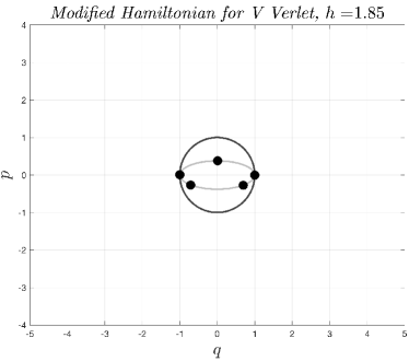
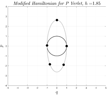
Figure 4.1: Modified Hamiltonian for velocity (left panel) and position (right panel) Verlet. The dots are the first five points along a discrete orbit of the velocity/position Verlet integrator initiated at $(q,p)=(1,0)$ and the gray line provides the associated level set of the modified Hamiltonian. For comparison, the black contour line shows the corresponding level set of the true Hamiltonian.

In particular numerical trajectories are contained in ellipses

$$\chi_{h}p^{2}+\frac{1}{\chi_{h}}q^{2}=\chi_{h}p_{0}^{2}+\frac{1}{\chi_{h}}q_{0}^{2}$$ (51)

rather than in circles (Figure 4.1).

Remark 4.2

A comparison of a given integrator (36) with (4) shows that

$$\left[\begin{matrix}q_{n+1}\\ p_{n+1}\end{matrix}\right]=\tilde{M}_{h}\left[\begin{matrix}q_{n}\\ p_{n}\end{matrix}\right],\qquad\tilde{M}_{h}=\left[\begin{matrix}A_{h}&-C_{h}\\ -B_{h}&D_{h}\end{matrix}\right]$$ (52)

is a second integrator of the same order of accuracy. We may think that (52) arises from (36) by changing the roles of the variables $q$ and $p$. In the particular case of splitting integrators, (52) arises from (36) after swapping the roles of the split systems $A$ and $B$. The integrators (36) and (52) share the same interval of stability and the same $\theta_{h}$. The function $\chi_{h}$ of (52) is obtained by changing the sign of the reciprocal of the function $\chi_{h}$ of (36). The important function $\rho(h)$ to be introduced in Proposition 6.7 is also the same for (36) and (52). The velocity Verlet algorithm and the position Verlet algorithm provide an example of this kind of pair of integrators (see Examples 3.3 and 3.4).

The results we have just presented may be extended to quadratic Hamiltonians with $d$ degrees of freedom (41): it is sufficient to use diagonalization as in Proposition 3.1. In particular, for stability we require that the stability interval of the integrator contains all products $h\omega_{i}$, where the frequencies $\omega_{i}$ are the square roots of the eigenvalues of $L^{-1}KL^{-T}$, with $LL^{T}=M$.

4.5 Optimal stability of Strang’s method

Let us fix an integer $N$ and consider consistent palindromic splitting integrators (33)–(34) with $s=N$; these use $N$ evaluations of $F$ per step when applied to problems of the form (23)–(24). The corresponding coefficient $A_{h}$ in (36) is a polynomial of degree $N$ in the variable $z=h^{2}$ (for obvious reasons $A_{h}$ is often called the stability polynomial of the integrator). We pointed out above that consistency imposes the relation $A_{h}=1-z/2+\mathcal{O}(h^{2})$. Our aim is to identify, among the class just described, the polynomial $A_{h}(z)$ that satisfies $|A_{h}(z)|<1$ for $0<h<h_{\rm max}$ with $h_{\rm max}$ as large as possible. As we shall show presently, the $A_{h}(z)$ sought corresponds to the integrator

$$\psi_{h}=\overbrace{\psi^{V}_{h/N}\circ\cdots\circ\psi^{V}_{h/N}}^{N{\rm times}},$$ (53)

where $\psi_{h}^{V}$ is the mapping associated with the Strang/Verlet formula (27). Note that to carry out a step of length $h$ with the method in (53) one just has to take $N$ consecutive steps of length $h/N$ of standard velocity Verlet. In other words, subject to stability, if one wishes to take as long a step as possible with a budget of $N$ evaluations of the force per step, the best choice is to concatenate $N$ steps of Strang/Verlet.

To see the optimality of $\psi_{h}$ in (53), we first note that, after expressing $\psi_{h/N}^{V}$ in terms of the $A$ and $B$ flows and merging consecutive $B$ flows, the mapping (53) corresponds indeed to a palindromic splitting with $N$ stages. Then, from Example 3.3 we know that Verlet is stable for $0<h<2$ and this implies that (53) is stable for $0<h/N<2$ (for (53) the powers of $\tilde{M}_{h}$ are powers of the Verlet matrix $\tilde{M}^{V}_{h/N}$). In this way (53) has stability interval $(0,2N)$ and we shall prove next that this is the longest possible. From Example (3.3), Verlet with step size $h/N$ has $A_{h/N}^{V}=1-h^{2}/(2N^{2})$, which, in view of (49)–(50), implies that for (53) the coefficient $A_{h}$ has the expression

$$\cos\theta_{h}=\cos(N\theta_{h/N}^{V}).$$

Recalling the definition $T_{N}(\cos\alpha)=\cos(N\alpha)$ of the Chebyshev polynomial $T_{N}$, we observe that for (53)

$$A_{h}(z)=T_{N}\big{(}1-\frac{z}{2N^{2}}\big{)}.$$

Well-known properties of $T_{N}$, imply that no other polynomial $A_{h}(z)$ of degree $\leq N$ with $A_{h}=1-z/2+\mathcal{O}(h^{2})$ has modulus $\leq 1$ in the interval $-1<1-z/(2N^{2})<1$, i.e. when $0<h<2N$.

5 Monte Carlo methods

In this section we review some basic concepts and principles of Monte Carlo methods aimed at computing integrals with respect to a given probability distribution (?, ?, ?, ?). We also describe the Hamiltonian or Hybrid Monte Carlo (HMC) method and some of its variants.

5.1 Simple Monte Carlo Methods

Given a probability distribution $\mu$ in $\mathbb{R}^{D}$ (the target distribution) and a function $F:\mathbb{R}^{D}\to\mathbb{R}$, the problem addressed by the algorithms considered here is to numerically estimate the following $D$-dimensional integral with respect to $\mu$,

$$\mu(F)=\int_{\mathbb{R}^{D}}F(x)\mu(dx)\;.$$ (54)

In general, $\mu(F)$ cannot be determined analytically. Moreover, since the dimension $D$ might not be small, conventional numerical quadrature is likely not to be practical or even feasible.

The simple Monte Carlo method approximately computes $\mu(F)$ in (54) by generating $N$ independent and identically distributed (i.i.d.) samples $X_{1},\dots,X_{N}$ from $\mu$, evaluating the function $F$ at these samples and using the estimator

$$\bar{F}_{N}=\frac{1}{N}\sum_{i=1}^{N}F(X_{i})\;.$$ (55)

Assuming that $\mu(F)<\infty$, the law of large numbers states that

$$\lim_{N\to\infty}\bar{F}_{N}=\mu(F)\quad\text{as $N\to\infty$},$$

almost surely. If, in addition, the standard deviation $\sigma_{0}(F)$ of the random variable $F(X)$, $X\sim\mu$, defined by

$$\sigma_{0}(F)^{2}=\int_{\mathbb{R}^{D}}(F(x)-\mu(F))^{2}\mu(dx)\;$$ (56)

is finite, the central limit theorem ensures the following distributional limit

$$N^{1/2}(\bar{F}_{N}-\mu(F))\overset{d}{\to}\mathcal{N}(0,\sigma_{0}(F)^{2})\quad\text{as}\quad N\to\infty.$$

Loosely speaking, this may be interpreted as stating that the distribution of $\bar{F}_{N}$ is approximately $\mathcal{N}(0,\sigma_{0}(F)^{2}/N)$. Hence, the standard deviation of the error $\bar{F}_{N}-\mu(F)$ decreases like the inverse square root of the number of samples. Often this standard deviation is referred to as Monte Carlo error. Thus, to halve the Monte Carlo error the number of i.i.d. samples needs to be quadrupled.

In most cases of practical interest, one cannot directly generate i.i.d. samples $X_{i}$ from $\mu$ and resorts to Markov Chain Monte Carlo methods.

5.2 Markov Chain Monte Carlo Methods

Recall that a Markov chain with state space $\mathbb{R}^{D}$ is a sequence of random $D$-vectors $\{X_{i}\}_{i\in\mathbb{N}}$ that satisfies the Markov property

$$\mathbb{P}(X_{i+1}\in A\mid X_{1},\dots,X_{i})=\mathbb{P}(X_{i+1}\in A\mid X_{i})$$

for all measurable sets $A$. In other words, given the past history of the chain $X_{1},\dots,X_{i}$, the only information required to update the state of the chain is the current state $X_{i}$. Here our interest is restricted to (time–)homogenuous chains, i.e. to cases where $\mathbb{P}(X_{i+1}\in A\mid X_{i})$ is independent of $i$.

Typically one constructs a homogeneous Markov chain in terms of its transition probabilities $\Pi_{x}$, $x\in\mathbb{R}^{D}$. These are the probabilities

$$\Pi_{x}(A)=\mathbb{P}(X_{i+1}\in A\mid X_{i}=x)\;,$$

with $i\in\mathbb{N}$ and $A$ measurable. Often $\Pi_{x}$ may be computed as

$$\Pi_{x}(A)=\int_{A}\Pi_{x}(dx^{\prime}),$$

for a suitable kernel $\Pi_{x}(dx^{\prime})$. Clearly the chain is determined once the transition probabilities and the distribution of $X_{1}$ are known. In practice, the term chain is used in a wide sense to refer to the transition probabilities without specifying the distribution of $X_{1}$.

A probability distribution $\nu$ is an invariant or stationary distribution of a Markov chain with transition probabilities $\Pi_{x}$ if

$$\int_{\mathbb{R}^{D}}\Pi_{x}(A)\nu(dx)=\int_{A}\nu(dx)$$

holds for all measurable sets $A$. We also say that $\Pi_{x}$ preserves $\nu$. In the situations we are interested in, a Markov chain will have a unique invariant distribution. If $\nu$ is the invariant distribution of the chain and in addition $X_{1}\sim\nu$, one says that the chain is at stationarity.

Markov Chain Monte Carlo (MCMC) methods generate a Markov chain $\{X_{i}\}_{i\in\mathbb{N}}$ that has the target $\mu$ as an invariant distribution and estimate $\mu(F)$ by the average (55). By analogy to the simple i.i.d. situation described above, one would like to have MCMC methods that meet two basic requirements.

• For each $F:\mathbb{R}^{D}\to\mathbb{R}$ such that $\mu(F)<\infty$,

  $$\bar{F}_{N}\overset{a.s.}{\to}\mu(F)\quad\text{as $N\to\infty$}\;.$$ (57)

  This is the MCMC analog of the law of large numbers.

• For each $F:\mathbb{R}^{D}\to\mathbb{R}$ such that $\mu(F)<\infty$ and $\sigma_{0}(F)<\infty$,

  $$N^{1/2}(\bar{F}_{N}-\mu(F))\overset{d}{\to}\mathcal{N}(0,\sigma(F)^{2})\quad\text{as $N\to\infty$},$$ (58)

  for some $\sigma(F)$. This is the MCMC analog of the central limit theorem.

For each fixed function $F$ and Markov chain $\{X_{i}\}_{i\in\mathbb{N}}$, the constant $\sigma(F)^{2}$ appearing in (58) is called the asymptotic variance of the MCMC estimator $\bar{F}_{N}$. A straightforward calculation shows that this asymptotic variance satisfies

$$\sigma(F)^{2}=\sigma_{0}(F)^{2}+2\sum_{i>1}\operatorname{cov}_{\mu}(F(X_{1}),F(X_{i}))$$

where $\sigma_{0}(F)$ is defined in (56) and the covariances are computed assuming that the chain is at stationarity. If the $X_{i}$ were independent, all the covariances $\operatorname{cov}_{\mu}(F(X_{1}),F(X_{i}))$ would vanish and we would recover the standard central limit theorem. Since in most interesting cases the $X_{i}$’s in the Markov chain are not mutually independent, often $\sigma(F)$ is larger than $\sigma_{0}(F)$. Generally speaking it is desirable to have low values of $\operatorname{cov}_{\mu}(X_{1},X_{i})$ so that $\sigma(F)$ is not far away from $\sigma_{0}(F)$ for each $F$.

In practice, the inputs that the user has to supply to an MCMC algorithm include, at least:

• A sample of the initial state $X_{1}$. Ideally, this sample should be taken in a domain of state space of high probability. Otherwise the chain may need many steps to start generating useful samples. A discussion of this issue is out of the scope of this paper.

• A, not necessarily normalized, density function $\rho$ of the target $\mu$ (i.e. the probability density function is $Z^{-1}\rho(x)$, where $Z=\int_{{\mathbb{R}}^{D}}\rho(x)dx$ is not assumed to be $1$; the value of $Z$ is not required to run the algorithms).

5.3 Metropolis Method for Reversible Maps

The replacement of the i.i.d. variables that simple Monte Carlo uses in the estimator (55) with variables of a Markov chain is of interest because it is not difficult to construct a chain that has a given target $\mu$ as an invariant distribution. The key of this construction is the Metropolis-Hastings accept/reject mechanism, that turns a given proposal chain (for which $\mu$ is not invariant) into a Metropolized chain, which leaves $\mu$ invariant. The simplest Metropolis rule was introduced in 1953 in a landmark paper (?); later Hastings provided an important generalization (?).

A review of the Metropolis-Hastings rule is not required for our purposes here. However we shall present a trimmed down variant of Metropolis-Hastings that we will use to define HMC. This variant works in the special case where the target $\mu$ is invariant with respect to a linear involution, takes as an input a reversible deterministic map and manufactures a Markov chain that preserves $\mu$. While the chain that we construct is not expected to satisfy a law of large numbers and therefore has no practical merit, Proposition 5.1 will be used later to analyse HMC methods.

The technique, patterned after (?), requires a non-normalized density function $\rho:\mathbb{R}^{D}\to\mathbb{R}$ of the target, and, as pointed out above, a map $\Phi:\mathbb{R}^{D}\to\mathbb{R}^{D}$ that is reversible with respect to a linear involution $S$ that preserves probability, i.e. $\rho\circ S=\rho$. The accept/reject mechanism is based on the acceptance probability $\alpha:\mathbb{R}^{D}\to[0,1]$ defined as

$$\alpha(x)=\min\left\{1,\frac{\rho(\Phi(x))}{\rho(x)}\left|\det\Phi^{\prime}(x)\right|\right\}.$$ (59)

($\Phi^{\prime}$ is the Jacobian matrix of $\Phi$.)

We consider the following algorithm:

Algorithm 5.1 (Metropolized Reversible Map)

Given $X_{0}\in\mathbb{R}^{D}$ (the input state), the method outputs a state $X_{1}$ as follows.

Step 1

Generate a proposal move $\tilde{X}_{1}=\Phi(X_{0})$.

Step 2

Output $X_{1}=\gamma\tilde{X}_{1}+(1-\gamma)S(X_{0})$ where $\gamma$ is a Bernoulli random variable with parameter $\alpha(X_{0})$ (i.e. $\gamma$ is $1$ with probabilty $\alpha(X_{0})$ and $0$ with probability $1-\alpha(X_{0})$).

Step 2 contains the accept/reject mechanism. In case of acceptance the updated state coincides with the state proposed $\tilde{X}_{1}$ from Step 1; in case of rejection the updated state is $S(X_{0})$. Note that, in case of rejection, conventional Metropolis mechanisms set the updated state of the chain to be $X_{0}$.

Proposition 5.1

In the situation described above, let $\{X_{i}\}_{i\in\mathbb{N}}$ be the Markov chain defined by iterating Algorithm 5.1. Then the target distribution is an invariant distribution of this chain.

Proof 5.1.

The transition kernel of $\{X_{i}\}_{i\in\mathbb{N}}$ is given by

$$\Pi_{x}(dx^{\prime})=\alpha(x)\delta(x^{\prime}-\Phi(x))dx^{\prime}+(1-\alpha(x))\delta(x^{\prime}-S(x))dx^{\prime}$$

where $\delta(\cdot)$ is the Dirac-delta function. Hence, for any measurable set $A$, if $1_{A}(x)$ denotes the corresponding indicator function,

$$\int_{\mathbb{R}^{D}} \Pi_{x}(A)\rho(x)dx=\int_{A}\rho(x)dx$$

$$+\int_{\mathbb{R}^{D}}\alpha(x)\rho(x)1_{A}(\Phi(x))dx-\int_{\mathbb{R}^{D}}\alpha(x)\rho(x)1_{A}(S(x))dx\;.$$

By change of variables in the third integral,

$$\int_{\mathbb{R}^{D}} \Pi_{x}(A)\rho(x)dx=\int_{A}\rho(x)dx$$

$$+\int_{\mathbb{R}^{D}}\alpha(x)\rho(x)1_{A}(\Phi(x))dx$$

$$-\int_{\mathbb{R}^{D}}\alpha\big{(}S(\Phi(x))\big{)}\left|\det\Phi^{\prime}(x)\right|\rho(\Phi(x))1_{A}(\Phi(x))dx,$$

where we used the hypothesis that $\rho\circ S=\rho$. The last two terms on the right-hand side of this equation cancel because

$$\alpha\big{(}S(\Phi(x))\big{)} =\min\left\{1,\frac{\rho(x)}{\rho(\Phi(x))}\left|\det\Phi^{\prime}(x)\right|^{-1}\right\}$$

$$=\alpha(x)\rho(x)\frac{1}{\rho(\Phi(x))}\left|\det\Phi^{\prime}(x)\right|^{-1},$$

which follows from the reversibility of $\Phi$, the hypothesis $\rho\circ S=\rho$ and Proposition 2.4.

5.4 The HMC method: basic idea

We consider a target distribution $\Pi$ in ${\mathbb{R}}^{d}$. If $\mathcal{U}:\mathbb{R}^{d}\to\mathbb{R}$ denotes the negative logarithm of the (not necessarily normalized) probability density function of the target, then

$$\Pi(dq)=Z_{q}^{-1}\exp(-\mathcal{U}(q))dq\;,\quad\text{where}\quad Z_{q}=\int_{\mathbb{R}^{d}}\exp(-\mathcal{U}(q))\,dq\;.$$

The Monte Carlo algorithms studied here use $\mathcal{U}$ but do not require the knowledge of the normalization factor $Z_{q}$. In HMC, regardless of the application in mind, $\mathcal{U}$ is seen as the potential energy of a mechanical system with coordinates $q$. Then auxiliary momenta $p\in{\mathbb{R}}^{d}$ and a quadratic kinetic energy function $\mathcal{T}(p)=(1/2)p^{T}M^{-1}p$ are introduced as in (10) ($M$ is a positive-definite, symmetric matrix chosen by the user). The total energy of this fictitious mechanical system is $H=\mathcal{T}+\mathcal{U}$ and the equations of motion are given in (9).

Example 5.2.

In the particular case where the target $\mu$ is Gaussian with un-normalized density $\exp(-(1/2)q^{T}Kq)$, $q\in{\mathbb{R}}^{d}$, we have $\mathcal{U}(q)=(1/2)q^{T}Kq$, which leads to the Hamiltonian (41) we discussed before. For a univariate standard normal target, $H=(1/2)(p^{2}+q^{2})$ and Hamilton’s equations reduce to those of harmonic oscillator (3).

The Boltzmann-Gibbs distribution in ${\mathbb{R}}^{2d}$ corresponding to $H$ was discussed earlier in connection with Theorem 2.3. This distribution is defined as (for simplicity the inverse temperature is taken here to be $\beta=1$):

$$\Pi_{BG}(dq,dp) =(2\pi)^{-\frac{1}{2}d}\left|\det{M}\right|^{-\frac{1}{2}}\exp\left(-\frac{1}{2}p^{T}M^{-1}p\right)$$

$$\qquad\qquad\qquad\qquad\qquad\times Z_{q}^{-1}\exp(-\mathcal{U}(q))dq\,dp.$$ (60)

Clearly the target $\Pi$ is the $q$–marginal of $\Pi_{BG}$. The $p$–marginal is Gaussian with zero mean and covariance matrix $M$; therefore samples from this marginal are easily available (and will be put to use in the algorithms below). A key fact for our purposes: Hamilton’s equations of motion (9) preserve $\Pi_{BG}$ (Theorem 2.3).

HMC generates (correlated) samples $(q_{i},p_{i})\in{\mathbb{R}}^{2d}$ by means of a Markov chain that leaves $\Pi_{BG}$ invariant; the corresponding marginal $q_{i}\in{\mathbb{R}}^{d}$ chain then leaves invariant the target distribution $\Pi$. The basic idea of HMC is encapsulated in the following algorithm (the duration $\lambda>0$ is a —deterministic— parameter, whose value is specified by the user).

Algorithm 5.2 (Exact HMC)

Let $\lambda>0$ denote the duration parameter.

Given the current state of the chain $(q_{0},p_{0})\in\mathbb{R}^{2d}$, the method outputs a state $(q_{1},p_{1})\in\mathbb{R}^{2d}$ as follows.

Step 1

Generate a $d$-dimensional random vector $\xi_{0}\sim\mathcal{N}(0,M)$.

Step 2

Evolve over the time interval $[0,\lambda]$ Hamilton’s equations (9) with initial condition $(q(0),p(0))=(q_{0},\xi_{0})$.

Step 3

Output $(q_{1},p_{1})=(q(\lambda),p(\lambda))$.

Note that $p_{0}$ plays no role, since the initial condition starts from $\xi_{0}$. Step 1 is referred to as momentum refreshment or momentum randomization.

It is easy to see that this algorithm succeeds in preserving the distribution $\Pi_{BG}$:

Theorem 5.3.

Consider the Markov chain $\{(q_{i},p_{i})\}_{i\in\mathbb{N}}$ defined by iterating Algorithm 5.2. The probability distribution $\Pi_{\operatorname{BG}}$ in (5.4) is an invariant distribution of this chain.

Proof 5.4.

The transformation $(q_{0},p_{0})\mapsto(q_{0},\xi_{0})$ obviously preserves the Boltzmann-Gibbs distribution. The same is true for the transformation $(q_{0},\xi_{0})\mapsto(q_{1},p_{1})$ as we saw in Theorem 2.3.

The transition kernel of this chain is given by

$$\Pi_{(q,p)}(dq^{\prime},dp^{\prime})=\mathbb{E}\left\{\delta((q^{\prime},p^{\prime})-\varphi_{\lambda}(q,\xi))\right\}dq^{\prime}dp^{\prime},$$

where the expected value is over $\xi\sim\mathcal{N}(0,M)$.

The most appealing feature of the algorithm is that, if $\lambda$ is sufficiently large, we may hope that the Markov transitions $i\rightarrow i+1$ produce values $q_{i+1}$ far away from $q_{i}$, thus reducing the correlations in the chain and facilitating the exploration of the target distribution.

5.5 Numerical HMC

Algorithm 5.2 cannot be used in practice because in the cases of interest the exact solution flow $\varphi_{\lambda}$ of Hamilton’s equations is not available. It is then necessary to resort to numerical approximations to $\varphi_{\lambda}$, but, as pointed out in Section 4, numerical methods cannot preserve volume in phase space and energy and therefore do not preserve exactly the Boltzman-Gibbs distribution. To correct the bias introduced by the time discretization error, the numerical solution is Metropolized using Algorithm 5.1. However, this requires that the numerical integrator be reversible.

Let $\Psi_{\lambda}$ denote a numerical approximation of $\varphi_{\lambda}$ (more precisely, if the step size is $h$ and $n=\lfloor\lambda/h\rfloor$ is the number of steps required to integrate up to $t=\lambda$, then $\Psi_{\lambda}=\psi_{h}^{n}$). In order to use Algorithm 5.1 with $\Psi_{\lambda}$ playing the role of $\Phi$ and the momentum flip involution (13) playing the role of $S$, we first note (Proposition 2.6) that the momentum flip involution preserves $H$ in (10) and, as a consequence, it preserves the Boltzmann-Gibbs distribution. In addition Theorem 2.4 ensures that the Hamiltonian flow is reversible with respect to this involution; it then makes sense (Theorem 4.2) to assume that the integrator chosen is such that $\Psi_{\lambda}$ is also reversible. The acceptance probability in (59) now reads

$$\alpha(q,p)=\min\left\{1,e^{-\Delta H(q,p)}\left|\det\Psi_{\lambda}^{\prime}(q,p)\right|\right\}\;,$$ (61)

where

$$\Delta H(q,p)=H(\Psi_{\lambda}(q,p))-H(q,p)$$

is the energy error (recall that if the integrator were exact $H(\Psi_{\lambda}(q,p))$ would coincide with $H(q,p)$ by conservation of energy, Theorem 2.2).

Algorithm 5.3 (Numerical HMC)

Denote by $\lambda>0$ the duration parameter and let $\Psi_{\lambda}$ be a reversible numerical approximation to the Hamiltonian flow $\varphi_{\lambda}$.

Given the current state of the chain $(q_{0},p_{0})\in\mathbb{R}^{2d}$; the method outputs a state $(q_{1},p_{1})\in\mathbb{R}^{2d}$ as follows.

Step 1

Generate a $d$-dimensional random vector $\xi_{0}\sim\mathcal{N}(0,M)$.

Step 2

Find $\Psi_{\lambda}(q_{0},\xi_{0})$ by evolving Hamilton’s equations (9) with a reversible integrator over the time interval $[0,\lambda]$ with initial condition $(q_{0},\xi_{0})$.

Step 3

Output $(q_{1},p_{1})=\gamma\Psi_{\lambda}(q_{0},\xi_{0})+(1-\gamma)(q_{0},-\xi_{0})$ where $\gamma$ is a Bernoulli random variable with parameter $\alpha(q_{0},\xi_{0})$ with $\alpha$ as in (61).

Theorem 5.5.

Consider the Markov chain $\{(q_{i},p_{i})\}_{i\in\mathbb{N}}$ defined by iterating Algorithm 5.3. The probability distribution $\Pi_{\operatorname{BG}}$ in (5.4) is an invariant distribution of this chain.

Proof 5.6.

As in the preceding theorem, the transformation $(q_{0},p_{0})\mapsto(q_{0},\xi_{0})$ preserves the Boltzmann-Gibbs distribution. The same is true for the transformation $(q_{0},\xi_{0})\mapsto(q_{1},p_{1})$ according to Proposition 5.1.

The transition kernel of the chain is given by

$$\Pi_{(q,p)}(dq^{\prime},dp^{\prime}) =\mathbb{E}\left\{\alpha(q,\xi)\delta((q^{\prime},p^{\prime})-\Psi_{\lambda}(q,\xi))\right\}dq^{\prime}dp^{\prime}$$

$$\qquad\qquad+\mathbb{E}\left\{(1-\alpha(q,\xi))\delta((q^{\prime},p^{\prime})-S(q,\xi))\right\}dq^{\prime}dp^{\prime}.$$

In practice, the acceptance probability (61) may not be readily available due to the need to compute $\det\Psi_{\lambda}^{\prime}(q,p)$. If the numerical approximation $\Psi_{\lambda}$ in addition to being assumed reversible is also volume preserving (as it would be for splitting integrators according to Theorem 4.1), then the determinant drops from the formula, and then the acceptance probability

$$\alpha(q,p)=\min\left\{1,e^{-\Delta H(q,p)}\right\}\;,$$ (62)

becomes easily computable. Variants where preservation of volume does not take place are studied by (?).

Remark 5.7.

The states of the Markov chain $\{(q_{i},p_{i})\}_{i\in\mathbb{N}}$ are not to be confused with the intermediate values of $q$ and $p$ that the numerical integrator generates while transitioning the chain from one state of the chain to the next. Those intermediate values were denoted by $(q_{n},p_{n})$ in the preceding sections and we have preferred not to introduce additional notation to describe the Markov chain.

Remark 5.8.

Theorems 5.3 and 5.5 show that $\Pi_{\rm BG}$ is an invariant distribution for the chains generated by Algorithms 5.2 and 5.3 respectively. However they do not guarantee that those chains meet the two basic requirements in (57) and (58) and indeed a simple example will be presented below where the sequence of values of $q$ generated by those algorithms is $q_{0}$, $-q_{0}$, $q_{0}$, $-q_{0}$, …so that the requirements are not met. A detailed study of the convergence properties of HMC is outside the scope of this paper and we limit ourselves to some remarks in Section 9.5.

5.6 Exact Randomized HMC

The Hamiltonian flow in Step 2 of Algorithm 5.2 is what, in principle, enables HMC to make large moves in state space that reduce correlations in the Markov chain $\{q_{i}\}_{i\in\mathbb{N}}$. Roughly speaking, one may hope that, by increasing the duration $\lambda$, $q_{1}$ moves away from $q_{0}$, thus reducing correlation. However, simple examples show that this outcome is far from assured.

Indeed, for the univariate standard normal target distribution in Example 5.2, the Hamiltonian flow is a rotation in the $(q,p)$-plane with period $2\pi$. It is easy to see that, if $q_{0}$ is taken from the target distribution, as $\lambda$ increases from $0$ to $\pi/2$, the correlation between $q_{1}$ and $q_{0}$ decreases and for $\lambda=\pi/2$, $q_{1}$ and $q_{0}$ are independent. However increasing $\lambda$ beyond $\pi/2$ will cause an increase in the correlation and for $\lambda=\pi$, $q_{1}=-q_{0}$ and the chain is not ergodic. For general distributions, it is likely that a small $\lambda$ will lead to a highly correlated chain, while choosing $\lambda$ too large may cause the Hamiltonian trajectory to make a U-turn and fold back on itself, thus increasing correlation (?). Generally speaking the performance of HMC may be very sensitive to changes in $\lambda$ as first noted by (?). In order to increase the robustness of the algorithm, Mackenzie suggested to vary randomly $\lambda$ from one Markov transition to the next and for that purpose he used a uniform distribution in an interval $[\lambda_{\rm min},\lambda_{\rm max}]$.

Recently (?) have studied an algorithm where the lengths of the time intervals of integration of the Hamiltonian dynamics at the different transitions of the Markov chain are independent and identically distributed exponential random variables with mean $\lambda$; these durations are of course taken to be independent of the state of the chain. The algorithm is then as follows:

Algorithm 5.4 (Exact RHMC)

Given the current state of the chain $(q_{0},p_{0})\in\mathbb{R}^{2d}$, the algorithm outputs the state $(q_{1},p_{1})\in\mathbb{R}^{2d}$ as follows.

Step 1

Generate a $d$-dimensional random vector $\xi_{0}\sim\mathcal{N}(0,M)$.

Step 2

Generate a random duration $t\sim\operatorname{Exp}(1/\lambda)$.

Step 3

Evolve over the time interval $[0,t]$ Hamilton’s equations (2) with initial condition $(q(0),p(0))=(q_{0},\xi_{0})$.

Step 4

Output $(q_{1},p_{1})=(q(t),p(t))$.

Analogous to Theorem 5.1, the probability distribution $\Pi_{\operatorname{BG}}$ in (5.4) is an invariant distribution of the Markov chain $\{(q_{i},p_{i})\}_{i\in\mathbb{N}}$ defined by iterating Algorithm 5.4. Analytical results and numerical experiments (?, §4-5) show that the dependence of the performance of the RHMC Algorithm 5.4 on the mean duration parameter $\lambda$ is simpler than the dependence of the performance of Algorithm 5.2 on its constant duration parameter.

5.7 Numerical Randomized HMC

Unfortunately, the complex dependence of correlation on the duration parameter $\lambda$ of Algorithm 5.2 is not removed by time discretization and is therefore inherited by Algorithm 5.3. For instance, for the univariate standard normal target, it is easy to check that if $\lambda$ is close to an integer multiple of $\pi$ and $h>0$ is suitably chosen, then a Verlet numerical integration will result, for each $q_{0}$, in $q_{1}=-q_{0}$ (a move that will be accepted by the Metropolis-Hasting step).

To improve its performance, Algorithm 5.3 is typically operated with values of $h$ that are randomized (?). Since, due to stability restrictions, explicit integrators cannot be used with arbitrarily large values of the time step, $h$ is typically chosen from a uniform distribution in an (often narrow) interval $(\Delta t_{\rm min},\Delta t_{\rm max})$. The number of time steps $N$ in each integration leg is kept constant and therefore the length of the integration intervals is random with a uniform distribution in $(N\Delta t_{\rm min},N\Delta t_{\rm max})$. Even after such a randomization, the fact remains that increasing the duration parameter will increase the computational cost of each integration leg and may impair the quality of the sampling.

Several modifications of Algorithm 5.4 that use numerical integration are suggested in (?). The most obvious of them approximates the Hamiltonian flow in Step 3 by a volume-preserving, reversible integrator (such as Verlet) operated with a fixed step size $h$ and with the number of integration steps $m$ at the different transitions of the Markov chain being independent and identically distributed geometric random variables with mean $\lambda/h$. These random numbers are of course taken to be independent of the state of the chain. As in Algorithm 5.3, one needs an accept-reject mechanism to remove the bias due to the energy errors introduced by this integrator.

Algorithm 5.5 (Numerical RHMC)

Denote by $\lambda>0$ the duration parameter and let $\psi_{h}$ be a reversible numerical approximation of the Hamiltonian flow $\varphi_{h}$.

Given the current state of the chain $(q_{0},p_{0})\in\mathbb{R}^{2d}$, the algorithm outputs the state $(q_{1},p_{1})\in\mathbb{R}^{2d}$ as follows.

Step 1

Generate a $d$-dimensional random vector $\xi_{0}\sim\mathcal{N}(0,M)$.

Step 2

Generate a geometric random variable $m$ supported on the set $\{1,2,3,...\}$ and with mean $\lambda/h$.

Step 3

Output $(q_{1},p_{1})=\gamma\psi_{h}^{m}(q_{0},\xi_{0})+(1-\gamma)(q_{0},-\xi_{0})$ where $\gamma$ is a Bernoulli random variable with parameter $\alpha$ defined as in (62).

Analogous to Theorem 5.2, the probability distribution $\Pi_{\operatorname{BG}}$ in (5.4) is an invariant distribution of the Markov chain $\{(q_{i},p_{i})\}_{i\in\mathbb{N}}$ defined by iterating Algorithm 5.5.

In the remainder of this paper the attention is focused on Algorithm 5.3. Experiments based on Algorithm 5.5 are reported in Section 8.2 and an example that illustrates the effects of randomization of $h$ and $\lambda$ is presented in Section 9.3.

6 Numerical integration and HMC

The computational work in HMC mainly stems from the cost of the evaluations of the force $-\nabla\mathcal{U}$ that are required in the numerical integration to be carried out at each transition of the Markov chain (Step 2 of Algorithm 5.3). If the dimension $d$ of $q$ is high, those evaluations are likely to be expensive; for instance, in a molecular dynamics study of a macromolecule with $N\gg 1$ atoms, $d=3N$ and each atom typically interacts with all others, so that the complexity of evaluating $-\nabla\mathcal{U}$ grows like $N^{2}$. As in any other numerical integration, the aim is to reach a target accuracy with the minimum possible complexity. Specific to the HMC scenario is the fact that, in the event of rejection in Step 3, the algorithm wastes all of the force evaluations used to compute $\Psi_{\lambda}(q,\xi)$. In addition, when a rejection occurs at a transition $i\rightarrow i+1$ of the Markov chain, the new value $q_{i+1}$ coincides with the old $q_{i}$, and this contributes to an increase in the correlations along the chain, which degrades the quality of sampling as pointed out when discussing the central limit theorem in (58). Since low acceptance rates are unwelcome and the acceptance probability (62) is a function of the energy error $\Delta H(q,p)=H(\Psi_{\lambda}(q,p))-H(q,p)$, it is important to perform the integration so as to have small energy errors. In this connection we recall from Section 4 that symplectic integrators conserve energy with errors that are $\mathcal{O}(h^{\nu})$ over exponentially long time intervals. In this way, the symplecticness of the integrator plays a dual role in HMC. On the one hand, it ensures conservation of volume, thereby making it possible to have the simple expression (62) for the acceptance probability. On the other hand, it ensures favourable energy errors even if the integration legs are very long.

An additional point: the sign of the error matters. Formula (62) shows that, if the integration starts from a point $(q,p)$ for which $\Delta<0$, then $\alpha=1$ leading to acceptance.

This section begins with a key result, Theorem 6.3, that shows that for reversible, volume preserving integrators the energy error is on average much smaller than one may have anticipated. After that we study in detail the model case of Gaussian targets and discuss the construction of integrators more efficient than Verlet.

6.1 Mean energy error

Step 2 in Algorithm 5.3 requires a volume-preserving, reversible integrator if (62) is to be used. As we shall discuss now, those geometric properties have a direct impact on the mean energy error. We begin with an auxiliary result (?, Lemma 3.3) that holds for any volume-preserving, reversible map.

Proposition 6.1.

Let $\Psi:\mathbb{R}^{2d}\to\mathbb{R}^{2d}$ be a bijection that is volume-preserving and reversible with respect to the momentum flip involution (13) and set $\Delta(q,p)=H(\Psi(q,p))-H(q,p)$. If $g$ is an odd real function of a real variable, then

$$\int_{\mathbb{R}^{2d}}g(\Delta(q,p))\,e^{-H(q,p)}dqdp=-\int_{\mathbb{R}^{2d}}g(\Delta(q,p))\,e^{-H(\Psi(q,p))}dqdp,$$

provided that one of the integrals exists. If $g$ is even, then

$$\int_{\mathbb{R}^{2d}}g(\Delta(q,p))\,e^{-H(q,p)}dqdp=\int_{\mathbb{R}^{2d}}g(\Delta(q,p))\,e^{-H(\Psi(q,p))}dqdp,$$

provided that one of the integrals exists.

Proof 6.2.

By a change of variables under the map $(q,p)\mapsto S(\Psi(q,p))$,

$$\int_{\mathbb{R}^{2d}}g(\Delta(q,p))e^{-H(q,p)}dqdp = \int_{\mathbb{R}^{2d}}g(\Delta(S(\Psi(q,p))))\,e^{-H(S(\Psi(q,p)))}dqdp$$

$$= \int_{\mathbb{R}^{2d}}g(-\Delta(q,p))\,e^{-H(\Psi(q,p))}dqdp,$$

where in the first step we used that both $S$ and $\Psi$ preserve volume and in the second we took into account that $S$ leaves $H$ invariant and that the reversibility of $\Psi$ implies

$$\Delta(q,p)=-\Delta(S(\Psi(q,p))).$$ (63)

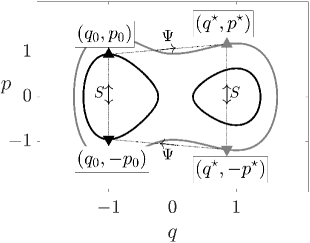
Figure 6.1: A univariate target with probability modes at $q=\pm 1$, leading to a double-well potential $\mathcal{U}$. The continuous lines are contours of constant $H$. The symmetry of the contours with respect to the axis $p=0$ is a consequence of the reversibility of the Hamiltonian flow. The solutions of Hamilton’s equations move from left to right when $p>0$ and from right to left when $p<0$, so when contours are reflected over the horizontal axis the arrow of time is reversed. If a reversible $\Psi$ maps $(q_{0},p_{0})$ into $(q^{*},p^{*})$, it has to map $(q^{*},-p^{*})$ into $(q_{0},p_{0})$, so as to preserve the symmetry of the figure. The transition $(q_{0},p_{0})\mapsto(q^{*},p^{*})$ has an increase in energy and $(q^{*},-p^{*})\mapsto(q_{0},p_{0})$ decreases energy in exactly the same amount; this is the content of formula (63).

We now use the proposition to bound the average of $\Delta$.

Theorem 6.3.

Let $\Psi:\mathbb{R}^{2d}\to\mathbb{R}^{2d}$ be a bijection that is volume-preserving and reversible with respect to the momentum flip involution (13). If the integral

$$m_{\Delta}=\int_{\mathbb{R}^{2d}}\Delta(q,p)e^{-H(q,p)}dqdp,$$ (64)

with $\Delta(q,p)=H(\Psi(q,p))-H(q,p)$, exists, then

$$0\leq m_{\Delta}\leq\int_{\mathbb{R}^{2d}}\Delta(q,p)^{2}e^{-H(q,p)}dqdp.$$ (65)

Furthermore the first inequality is strict except in the trivial case where $\Delta(q,p)$ vanishes for each $(q,p)$.

Proof 6.4.

By using the preceding proposition with $g(x)=x$, we get

$$m_{\Delta}=\frac{1}{2}\int_{\mathbb{R}^{2d}}\Delta(q,p)\left(1-e^{-\Delta(q,p)}\right)e^{-H(q,p)}dqdp\;.$$ (66)

The inequality $x(1-e^{-x})>0$, valid for all real $x\neq 0$, yields the lower bound in (65).

For the upper bound, we apply the inequality $|e^{x}-1|\leq|x|(e^{x}+1)$, valid for all $x\in\mathbb{R}$, to obtain

$$m_{\Delta} \leq\frac{1}{2}\int_{\mathbb{R}^{2d}}\left|\Delta(q,p)\right|\left|1-e^{-\Delta(q,p)}\right|e^{-H(q,p)}dqdp$$

$$\leq\frac{1}{2}\int_{\mathbb{R}^{2d}}\Delta(q,p)^{2}\left(1+e^{-\Delta(q,p)}\right)e^{-H(q,p)}dqdp$$

$$\leq\int_{\mathbb{R}^{2d}}\Delta(q,p)^{2}e^{-H(q,p)}\,dqdp.$$

In the last step we used the Proposition 6.1 with $g(x)=x^{2}$.

Figure 6.1 illustrates the geometry behind formula (63). The figure makes clear that to each initial condition $(q_{0},p_{0})$ with an energy increase $\Delta\geq 0$ there corresponds an initial condition $(q^{*},-p^{*})$ with an energy decrease of the same magnitude. In the integrand in (64) the energy increase at $(q_{0},p_{0})$ is weighed by $\exp(-H(q_{0},p_{0}))$, a larger factor than the weight $\exp(-H(q^{*},-p^{*}))$ of the corresponding energy decrease. In addition, by conservation of volume, if $(q_{0},p_{0})$ ranges in a small domain, then the corresponding points $(q^{*},-p^{*})$ range in a small domain of the same measure. This explains why the integral (64) is positive.

We are of course interested in applying Theorem 6.3 to the case where $\Psi$ is the map $\Psi_{\lambda}$ in Step 2 of the HMC Algorithm 5.3. Assume for simplicity that $\lambda/h$ is an integer, so that $t=\lambda$ coincides with one of the step points of the numerical integration. Then the energy error satisfies pointwise, i.e.  at each fixed $(q,p)$,

$$\Delta(p,q)=H(\Psi_{\lambda}(q,p))-H(q,p)=\big{[}H(\varphi_{\lambda}(q,p))+\mathcal{O}(h^{\nu})\big{]}-H(q,p)=\mathcal{O}(h^{\nu}),$$

where $\nu$ is the order of the integrator and we have successively used the convergence result in Theorem 3.1 and conservation of energy (Theorem 2.2). The bounds in Theorem 6.3 have important implications.

• The upper bound. Even though pointwise, the energy error $\Delta$ is of size $\mathcal{O}(h^{\nu})$, on average (with respect to the Boltzmann-Gibbs distribution) $m_{\Delta}$ is, at least formally, of size $\mathcal{O}(\Delta^{2})=\mathcal{O}(h^{2\nu})$. The order of the average energy error is automatically twice what we would have expected. This is clearly a pro of using a volume-reserving, reversible integrator.

• The lower bound. This is a con. Imagine a case where two uncoupled systems with Hamiltonian functions $H_{1}$ and $H_{2}$ are juxtaposed. The aggregate is a new Hamiltonian system with Hamiltonian $H_{1}+H_{2}$. The mean energy error for the aggregate is $\mathbb{E}(\Delta_{1}+\Delta_{2})=\mathbb{E}(\Delta_{1})+\mathbb{E}(\Delta_{2})$ and because both terms being added are $\geq 0$ there is no room for cancelation. In general, the value of the energy and therefore the value of the energy error may be expected to increase as the number of degrees of freedom increases, in agreement with the fact that in Physics energy is an extensive quantity.

This discussion will be continued in Section 7.

6.2 Energy error in the standard Gaussian target

Sections 3.4 and 4.4 were devoted to investigating the behaviour of different integrators when applied to the harmonic oscillator. We take up this theme once more, this time in the HMC context. The aim is then to study what happens when HMC is used to sample from the univariate standard normal, hoping that any findings will be relevant to more complex distributions. (Of course in practice there is no interest in using a MCMC algorithm to sample from a normal distribution. See the discussion on model problems at the beginning of Section 3.4.)

6.2.1 Pointwise energy error bounds

We return to the situation in Proposition 4.1 and now study the energy error after $n$ time-steps $\Delta(q_{0},p_{0})=H(p_{n},q_{n})-H(q_{0},p_{0})$, with $H=(1/2)(p^{2}+q^{2})$. The following result (?, Proposition 4.2) provides an upper bound for $\Delta(q_{0},p_{0})$ uniform in $n$.

Proposition 6.5.

The energy error, $\Delta(q_{0},p_{0})$, may be bounded as

$$\Delta(q_{0},p_{0})\leq\frac{1}{2}(\chi_{h}^{2}-1)p_{0}^{2},$$

if $\chi_{h}^{2}\geq 1$ or as

$$\Delta(q_{0},p_{0})\leq\frac{1}{2}\left(\frac{1}{\chi_{h}^{2}}-1\right)q_{0}^{2},$$

if $\chi_{h}^{2}\leq 1$.

Proof 6.6.

We only prove with the first item; the other is similar. The ellipse (51) has its major axis along the co-ordinate axis $p=0$ of the $(q,p)$ plane, as in the left panel of Figure 4.1. Hence $2H(q,p)=p^{2}+q^{2}$ attains its maximum on that ellipse if $p=0$ which implies $q^{2}=q_{0}^{2}+\chi_{h}^{2}p_{0}^{2}$. If the final point $(q_{n},p_{n})$ of the numerical trajectory happens to be at that maximum, $2\Delta(q_{0},p_{0})=(q_{0}^{2}+\chi_{h}^{2}p_{0}^{2})-(q_{0}^{2}+p_{0}^{2})$.

6.2.2 Average energy error bounds

We estimate next the average energy error (?, Proposition 4.3). Note that the bound provided is once more uniform in $n$.

Proposition 6.7.

In the situation described above, assume that $(q_{0},p_{0})$ is a Gaussian random vector with non-normalized probability density function $\exp(-H(q,p))$, with $H=(1/2)(p^{2}+q^{2})$. Then the expectation of the random variable $\Delta(q_{0},p_{0})\in{\mathbb{R}}^{2}$ is given by

$$\mathbb{E}(\Delta)=\sin^{2}(n\theta_{h})\>\rho(h),$$

where

$$\rho(h)=\frac{1}{2}\left(\chi_{h}^{2}+\frac{1}{\chi_{h}^{2}}-2\right)=\frac{1}{2}\left(\chi_{h}-\frac{1}{\chi_{h}}\right)^{2}\geq 0,$$

and accordingly

$$0\leq\mathbb{E}(\Delta)\leq\rho(h).$$

.

Proof 6.8.

With the shorthand $c=\cos(n\theta_{h})$, $s=\sin(n\theta_{h})$, we may write

$$2\Delta(q_{0},p_{0})=\left(-\frac{1}{\chi_{h}}sq_{0}+cp_{0}\right)^{2}+\big{(}cq_{0}+\chi_{h}sp_{0}\big{)}^{2}-\big{(}p_{0}^{2}+q_{0}^{2}\big{)}$$

or

$$2\Delta(q_{0},p_{0})=s^{2}\left(\frac{1}{\chi_{h}^{2}}-1\right)q_{0}^{2}+2cs\left(\chi_{h}-\frac{1}{\chi_{h}}\right)q_{0}p_{0}+s^{2}\big{(}\chi_{h}^{2}-1\big{)}p_{0}^{2}.$$

Since $\mathbb{E}(q_{0}^{2})=\mathbb{E}(p_{0}^{2})=1$ and $\mathbb{E}(q_{0}p_{0})=0$, the proof is ready.

6.2.3 Energy error bounds for Verlet

Let us illustrate the preceding results in the case of the Verlet integrator. For the velocity version, we find from Example 3.3 and (48), for $0<h<2$,

$$\chi_{h}^{2}=\frac{h^{2}}{1-\left(1-\frac{h^{2}}{2}\right)^{2}}=\frac{1}{1-\frac{h^{2}}{4}}>1.$$

The bound in Proposition 6.5 reads

$$\Delta(q_{0},p_{0})\leq\frac{h^{2}}{8(1-\frac{h^{2}}{4})}\>p_{0}^{2}.$$ (67)

For $h=1$, $\Delta(q_{0},p_{0})\leq p_{0}^{2}/6$; therefore, if $-2<p_{0}<2$ (an event that for a standard normal distribution has probability $>95\%$), then $\Delta(q_{0},p_{0})<2/3$ which results in a probability of acceptance $\geq 51\%$, regardless of the number $n$ of time-steps.

The position Verlet integrator (Example 3.4 and Remark 4.2) has $\chi_{h}^{2}=1-h^{2}/4<1$ provided that $0<h<2$. Proposition  6.5 yields

$$\Delta(q_{0},p_{0})\leq\frac{h^{2}}{8(1-\frac{h^{2}}{4})}\>q_{0}^{2}$$

(as one may have guessed from (67) by symmetry).

From Proposition 6.7, for both the velocity and the position versions,

$$0\leq\mathbb{E}(\Delta)\leq\rho(h)=\frac{h^{4}}{32(1-\frac{h^{2}}{4})}.$$ (68)

We draw the attention to the exponent of $h$ in the numerator: even though, pointwise, for the harmonic oscillator, energy errors for the Verlet integrator are $\mathcal{O}(h^{2})$, they are $\mathcal{O}(h^{4})$ on average, which of course matches our earlier finding in Theorem 6.3. For $h=1$ the expected energy error is $\leq 1/24$. Halving $h$ to $h=1/2$, leads to an expected energy error $\leq 1/480$. The conclusion of the examples above is that acceptance rates for Verlet are likely to be high even if the step size $h$ is not small.

6.3 Velocity Verlet or position Verlet?

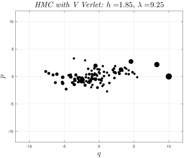
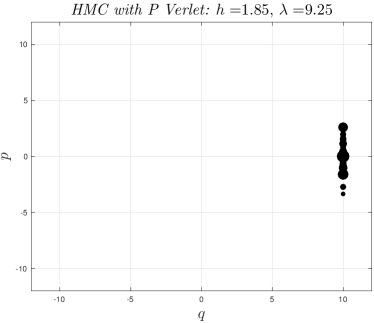
Figure 6.2: Discrete trajectories of the Markov chain when HMC for the standard Gaussian target is operated with velocity (left panel) and position (right panel) Verlet. Each marker is a state of the Markov chain (intermediate values of $(q,p)$ along the numerical trajectories are not depicted). The size of the markers is related to the index $i$ in the chain: states corresponding to larger values of $i$ have smaller markers. The chains start at $q=10$. On the right, all chain transitions result in rejection, so that $q_{i}=10$ for all values of $i$; position Verlet gets stuck. On the left, the velocity chain quickly identifies the interval around $q=0$ where the target distribution is concentrated.

The symmetry between the velocity and position Verlet integrators may lead to the conclusion that their performances in the HMC scenario are equivalent. This is not the case, because in Algorithm 5.3 (for a general target distribution) the $q$ and $p$ variables do not play a symmetric role at all. In particular, samples of $p$ from the correct marginal distribution (Step 1) are used as initial conditions for the integration legs in Step 2. On the contrary, when the Markov chain is initialized, the user has to guess a suitable starting value for $q$ (see the end of Section 5.2). In some applications, the chosen starting value may actually correspond to a location of low probability, and we now study the difficulties that may arise in that case.

Figure 6.2 corresponds to the standard Gaussian/harmonic oscillator target and compares the performance of the velocity and position algorithms when the chain is initialized with $q$ at a location of very low probability, $q_{0}=10$, ten standard deviations away from the mean (the initialization of $p$ is of no consequence since momenta are discarded in the momentum–refreshment Step 1 of Algorithm 5.3). The position integrator gets stuck where its velocity counterpart succeeds without problems.

Insight into the different behaviors of velocity and position Verlet may be gained from Figure 6.3, that corresponds to integrations with the large value $h=1.85$ carried out in the interval $0\leq t\leq\lambda=9.25$ (five time-steps). Regardless of the choice of $|q_{0}|$, velocity Verlet will result in an energy decrease (and therefore in acceptance) if the initial sample $\xi_{0}$ of the momentum is such that $(q_{0},\xi_{0})$ lands in the grey area of the left panel, which will happen with large probability because small values of $|\xi_{0}|$ are likely to occur. On the contrary, in the position algorithm energy decreases only occur if very large values of $\xi_{0}$ are drawn. Certainly, there is symmetry between the gray areas of both panels; however, in HMC, having energy decreases near the $q$ axis is helpful and having them near the $p$ axis is not. It may help to go back to the bound (67) that shows that, for velociy Verlet, $p_{0}=0$ ensures an energy decrease; compare both panels in Figure 4.1 as well.

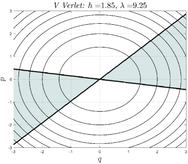
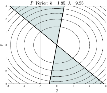
Figure 6.3: Regions where the energy error $\Delta(q,p)$ is positive/negative for velocity (left panel) and position (right panel) Verlet. In the gray-shaded regions $\Delta(q,p)$ is negative, ensuring acceptance of the Markov transition. The contour lines in the background shows level sets of $H(q,p)$.

To conclude this discussion we emphasize that if the chains were initialized by drawing samples from the marginal distribution of $q$ (i.e. started at stationarity), then the behaviour of velocity and position Verlet would be the same due to the $q/p$ symmetry.

6.4 Multivariate Gaussian model

We study once more the quadratic Hamiltonian (41) and note that the covariance matrix $\Sigma$ of the target is the inverse of the stiffness matrix $K$. As discussed in Proposition 3.1, in the particular case where $M=I$, the square roots of the eigenvalues of $K$ are the angular frequencies of the dynamics; the eigenvalues of $\Sigma$ are of course the variances of the target along the directions of the eigenvectors. Thus small variance implies high frequency.

6.4.1 Average energy error in the multivariate case

Proposition 6.7 may be extended to the multivariate Gaussian case. We begin by providing a variant of Proposition 3.1.

Proposition 6.9.

The change of dependent variables, $q=L^{-T}U\Omega^{-1}Q$, $p=LUP$, decouples the system into a collection of $d$ harmonic oscillators (superscripts denote components):

$$\frac{dQ^{i}}{dt}=\omega_{i}P^{i},\qquad\frac{dP^{i}}{dt}=-\omega_{i}Q^{i},\qquad i=1,\dots,d.$$

In terms of the new variables, the function in (41) is given by

$$\frac{1}{2}P^{T}P+\frac{1}{2}Q^{T}Q=\frac{1}{2}\sum_{i}\big{(}(P^{i})^{2}+(Q^{i})^{2}\big{)}.$$

Therefore the $2d$ variables $Q^{i}$ and $P^{i}$ are independent standard Gaussian.

As discussed in connection with Proposition 3.1, we may assume that the numerical method is applied to each of the uncoupled oscillators. After recalling Remark 3.6, the following result is easily proved.

Theorem 6.10.

Consider a stable integration of (41) with a (consistent), reversible, volume preserving integrator applied with a stable value of $h$. If $(q_{0},p_{0})$ are random variables with probability density function (proportional to) $\exp(-H)$, then for each $n$ the expectation of the energy error $\Delta(q_{0},p_{0})=H(q_{n},p_{n})-H(q_{0},p_{0})$ may be bounded as

$$0\leq\mathbb{E}(\Delta)\leq\sum_{j=1}^{d}\rho(\omega_{j}h),$$ (69)

where $\rho$ is the function defined in Proposition 6.7.

6.4.2 An illustration

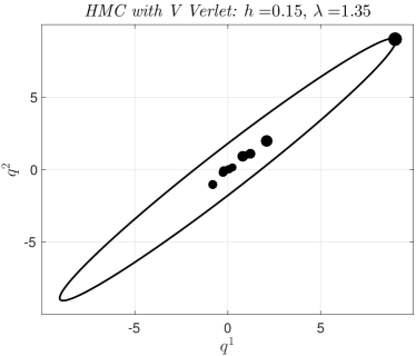
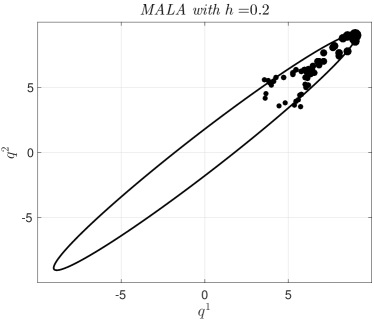
Figure 6.4: Bivariate Gaussian distribution, $(q^{1},q^{2})$ plane; the ellipse is a contour of constant probability density. HMC operated with velocity Verlet (left panel) and MALA (right panel). The size of the markers is related to $i$: points along the Markov trajectory corresponding to larger values of $i$ have smaller markers. The computational budget for both algorithms is fixed at 100 force evaluations. Along these trajectories, the average acceptance probability for HMC and MALA is 93% and 82%, respectively. The stability requirement for Verlet is $h<0.2$, which is set by the component of the target distribution with the smallest variance. In relation to MALA, note that HMC relaxes faster to a region of high probability.

As an example, we consider a two-dimensional target where

$$K=\Sigma^{-1}=\frac{1}{2}\begin{bmatrix}101&-99\\ -99&101\end{bmatrix}$$

This matrix has eigenvalues $\omega_{1}^{2}=1$ (with eigenspace $q^{1}=q^{2}$) and $\omega_{2}^{2}=100$ (with eigenspace $q^{1}=-q^{2}$). The mass matrix is chosen to be $M=I$. We use HMC with velocity Verlet; stability requires $h\omega_{2}<2$ or $h<0.2$ and we set $h=0.15$. The chain is started at $(q^{1},q^{2})=(9,9)$ where $\mathcal{U}(9,9)=81$, i.e. about 9 standard deviations in the direction of largest variance. The duration parameter $\lambda$ is set to be equal to 1.35 (i.e. there are $9$ time-steps in each numerical integration leg) and the number of transitions in the chain was the maximum attainable with a computational budget of 100 force evaluations. The left panel in Figure 6.4 shows that HMC rapidly relaxes to a region of high probability.

Remark 6.11.

It may be of interest to relate this experiment to the discussion of stiffness in Example 3.6. Here it is the oscillation with frequency $\omega_{1}$ (i.e. the evolution along the diagonal $q^{1}=q^{2}$) that matters most; however $h$ has to be chosen in terms of the oscillation with frequency $\omega^{2}$. Nevertheless HMC succeeds because, at each Markov transition, several time-steps are taken.

As a comparison we have also implemented the well-known algorithm MALA, with the same initial state and same computational budget. MALA may be described as the algorithm that results when, in HMC operated with velocity Verlet, the duration parameter $\lambda$ is chosen to coincide with $h$, i.e. each integration leg only takes one time-step. In this way the accept/reject mechanism operates after each individual time-step in MALA (but only after $\lambda/h$ successive time-steps in HMC). The right panel shows MALA zigzags in a region of low probability.

Remark 6.12.

In connection with the preceding remark, we note that for MALA the progress of the Markov chain along the $q^{1}=q^{2}$ diagonal is slow. Each time-step moves the state by a small amount, because $h$ was chosen by taking into account the behaviour of the problem along the $q^{1}=-q^{2}$ diagonal. The momentum refreshments, which in MALA take place after every individual time-step, change the direction of motion in the $(q^{1},q^{2})$ plane, thus inducing a random-walk behaviour. HMC avoids this random walk behaviour by taking sufficiently many time-steps between consecutive accept/reject steps so that integration legs make substantial strides in the solution components with high variance.

6.5 May Verlet be beaten?

Currently, velocity Verlet is the integrator of choice within HMC algorithms. Is this the best possibility? In this subsection we will discuss whether it is possible to construct a palindromic splitting formula with $s>1$ stages (33)–(34) that improves on the velocity Verlet algorithm in the sense that, when operated with a step size $h$, leads to smaller energy errors —higher acceptance probabilities— than velocity Verlet with step size $h/s$. Because, as illustrated above, Verlet is often very successful for large values of the step size, such a construction has to be based on investigating the behaviour of the integrators for finite $h$ and therefore cannot be guided by information (such as the expansion in Theorem 4.3) that corresponds to the behaviour as $h\to 0$. We therefore resort to Gaussian models with Hamiltonian of the form (41). In the remainder of this subsection we shall use the symbol $\tau$ to refer to the actual value of the step size implemented in the algorithm and keep the letter $h$ for the (nondimensional) product $\omega\tau$, where $\omega$ represents one of the frequencies present in the problem. With this notation, Verlet is stable for $0<h<2$ or $0<\tau<2/\omega_{\rm max}$.

When the number $d$ of degrees of freedom equals 1, velocity Verlet is indeed the best choice. We know, from Section 6.2, that Verlet will deliver high acceptance rates for $h$ just below its stability limit and, from Section 4.5, that Verlet has the longest stability interval. So Verlet peforms well for HMC for values of $\tau$ where other integrators are not even stable. Essentially the same is true for $d$ small, as one sees by decoupling the problem into $d$ one-degree-of-freedom oscillators as we did in Section 6.4. However, as $d$ increases, Verlet is not likely to keep high acceptance rates if $\tau$ is just below $2/\omega_{\rm max}$: in fact the additive character of the energy, noted in the discussion of Theorem 6.3, implies that, even if the energy error in each of the one-dimensional oscillators in the problem is small, the energy error for the overall system will likely be large. In that scenario, where, on accuracy grounds, Verlet has to be operated with $\tau$ significantly smaller than the stability limit $2/\omega_{\rm max}$, there is room for improvements in efficiency by resorting to more sophisticated integrators, as we discuss next.

6.5.1 Two stages

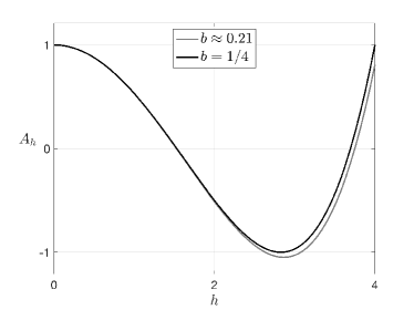
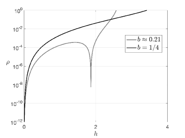
Figure 6.5: Two-stage palindromic integrators (31) corresponding to $b=1/4$ or $b$ given by (70). Left panel: stability polynomial $A_{h}$. For $b=1/4$ (which provides two steps of velocity Verlet of step length $\tau/2$) stabilty is lost at $h=4$ and there is a double root of the equation $A_{h}=-1$. The method (70) has a significantly shorter stability interval because under perturbation the double root of $A_{h}=-1$ splits into two real roots. Right panel: the quantity $\rho=\rho(h)$ that governs the expected energy error for Gaussian problems (see (69)). When the methods are operated with $0<h<2$, i.e. $0<\tau<2/\omega_{\rm max}$, the choice (70) yields values of $\rho$ much smaller than those corresponding to $b=1/4$.

We begin by studying the one-parameter family (31) of methods with two stages (i.e. essentially two force evaluations per step). For the choice $b=1/4$, one step of length $\tau$ of the two-stage method is equivalent to two steps of length $\tau/2$ of velocity Verlet (see equation (53) with $N=2$). The stability polynomial $A_{h}$ was described in terms of the Chebyshev polynomial $T_{2}$ in Section 4.5 and its graph may be seen in the left panel of Figure 6.5. Stability is lost at $h=4$ when $A_{h}=1$; at $h=2\sqrt{2}\approx 2.82$, there is a double root of the equation $A_{h}=-1$ (corresponding to the double root at $\zeta=0$ of the equation $T_{2}(\zeta)=2\zeta^{2}-1=-1$). Small perturbations of $b=1/4$ turn the double root of the equation $A_{h}=-1$ into two real roots in the neigbourhood of $h=2\sqrt{2}$; after such perturbation the length of the stability interval drops from 4 to $\approx 2\sqrt{2}$. Accordingly, in problems where $d$ is small enough for standard velocity Verlet to work well with $\tau\omega_{\rm max}$ in the interval $(\sqrt{2},2)$, no two-stage formula with $b\neq 1/4$ can improve upon Verlet. However if, when applying Verlet, $\tau\omega_{\rm max}$ has to be chosen below $\sqrt{2}$ on accuracy grounds, then, as we will see now, efficiency may be improved by choosing $b$ in (31) different from $1/4$.

The paper (?) suggests the following procedure to find the value of $b$. Numerical experiments in that reference show that, for Gaussian problems with $d\leq 1000$, (one-stage) velocity Verlet achieves acceptance rates $\geq 20\>\%$ when $\tau\omega_{\rm max}\leq 1$ (i.e. when $\tau$ is less than a half of the maximum allowed by stability). It is then assumed that two-stage integrators should be demanded to perform well when $\tau\omega_{\rm max}\leq 2$. On the other hand, in view of (69), for Gaussian models performance is governed by the quantity $\rho$ defined in Proposition 6.7, which for the one-parameter family (31) is found to be

$$\rho(h;b)=\frac{h^{4}\big{(}2b^{2}(1/2-b)h^{2}+4b^{2}-6b+1\big{)}^{2}}{8\big{(}2-bh^{2}\big{)}\big{(}2-(1/2-b)h^{2}\big{)}\big{(}1-b(1/2-b)h^{2}\big{)}}.$$

Then $b$ is chosen by minimizing

$$\|\rho\|_{(2)}=\max_{0\leq h\leq 2}\rho(h;b);$$

which yields $b=0.21178\dots$ To avoid cumbersome decimal expressions, (?) instead uses the approximate value

$$b=\frac{3-\sqrt{3}}{6}\approx 0.21132,$$ (70)

which gives $\|\rho\|_{(2)}\approx 5\times 10^{-4}$. For comparison $b=1/4$ has a substantially larger $\|\rho\|_{(2)}\approx 4\times 10^{-2}$. Numerical experiments reported in (?) confirm that, when $d$ is not small the method (70) is a clear improvement on Verlet in an example where the target is not Gaussian. See also (?).

6.5.2 Three stages

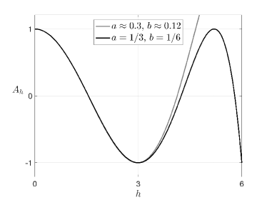
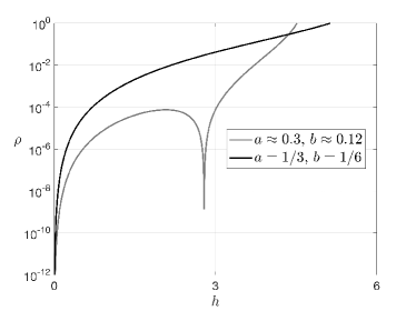
Figure 6.6: Three-stage palindromic integrators (32) for $a=1/3$, $b=1/6$ or $a$, $b$ given by (71). Left panel: stability polynomial $A_{h}$. Right panel: the quantity $\rho=\rho(h)$ that governs the expected energy error for Gaussian problems (see (69)). When the methods are operated with $0<h<3$, the choice (71) yields values of $\rho$ much smaller than those corresponding to $a=1/3$, $b=1/6$.

A similar study may be undertaken for the three-stage family (32) with two parameters $a$ and $b$. The choice $a=1/3$, $b=1/6$ yields a method consisting of the concatenation of three successive steps of length $\tau/3$ of velocity Verlet (see equation (53) with $N=3$). The graphs of the stability polynomial $A_{h}$ may be seen in the left panel of Figure 6.6. Stability is lost at $h=6$ when $A_{h}=-1$. The double root of $T_{3}(\zeta)=4\zeta^{3}-4\zeta=1$ at $\zeta=-1/2$ gives rise to a double root of $A_{h}=1$ at $h=3\sqrt{3}\approx 5.19$. The double root of $T_{3}(\zeta)=-1$ gives rise to a double root of $A_{h}=-1$ at $h=3$. Perturbing the values $a=1/3$, $b=1/6$ leads in general to methods with (short) stability intervals of length $\approx 3$, because typically the double root of $A_{h}=-1$ splits into two single roots. However it is possible to perturb $a$ and $b$ in such a way that, after perturbation, $A_{h}=-1$ has a double root close to $h=3$ as analyzed in (?). For such particular perturbations, stability is lost by crossing the line $A_{h}=1$. This is what happens for the choice

$$a=0.29619504261126,\quad b=0.11888010966548,$$ (71)

found in (?) by minimizing

$$\|\rho\|_{(3)}=\max_{0\leq h\leq 3}\rho(h;b).$$

Note that the range of the maximum is now ${0\leq h\leq 3}$ to account for the fact that, when using three force evaluations per step, we aim at integrations with $\tau\omega_{\rm max}\leq 3$ to be competitive with Verlet. The choice (71) results in $\|\rho\|_{(3)}\approx 7\times 10^{-5}$ and a stability interval of length $\approx 4.67\dots$ The paper (?) reports experiments that show the superiority of (71) over standard velocity Verlet and also describes the construction of optimized four-stage integrators.

6.5.3 The AIA approach

Let us go back to the one-parameter family (31) of methods with two stages. The choice (70) is based on the assumption that with $b=1/4$ the integrator (equivalent to velocity Verlet) would be used with $\tau\omega_{max}$ in the interval $(0,2)$. There is of course a degree of arbitrariness in the choice of this interval. When an interval $(0,c)$ with $c$ slightly above $2$ is considered, then minimization of

$$\max_{0\leq h\leq c}\rho(h;b)$$ (72)

results in a value of $b$ slightly above that corresponding to $(0,2)$. This improves the length of the stability interval, but, with the notation in Theorem 4.3, increases the quantity $C_{2,1}^{2}+C_{2,2}^{2}$, so that the integrator becomes less accurate in the limit $h\to 0$ (note that $C_{1,1}=0$ because we are dealing with methods of order 2). As $c$ is increased further, the value of $b$ that minimizes (72) increases towards $b=1/4$; the stability interval improves and accuracy worsens. For $c\geq 2\sqrt{2}$ the optimization procedure leads to $b=1/4$ because, as pointed out earlier, then $b=1/4$ is the only value for which the maximum in (72) is finite. On the other hand, as $c$ decreases from $2$, the optimal value of $b$ decreases, accuracy in the limit $h\to 0$ improves and the stability interval becomes shorter. In the limit $c\downarrow 0$, $b$ approaches $b\approx 0.1932$, the value that minimizes $C_{2,1}^{2}+C_{2,2}^{2}$ (?).

In the Adaptive Integration Approach (AIA) suggested by (?, ?) for molecular dynamics problems, the value of $b$ in (31) is chosen by minimizing (72) with the parameter $c$ adapted to the problem being solved, rather than being kept at the somehow arbitrary value $c=2$. The procedure is the following. In molecular dynamics packages such as GROMACS (?), the user is prompted to specify her choice of the value of $\tau$; of course smaller values of $\tau$ lead to more expensive simulations. The package estimates the values of the frequencies of all harmonic forces present in the problem and will not run if $\tau\tilde{\omega}_{\rm max}$ is close to the Verlet stability limit ($\tilde{\omega}_{\rm max}$ is the maximum of the estimated frequencies). AIA sets $c=\sqrt{2}\tilde{\omega}_{max}\tau$ ($\sqrt{2}$ is a safety factor) so that in (72) $h$ ranges in the shortest interval that contains all products $\sqrt{2}\tau\tilde{\omega}_{i}$, where $\tilde{\omega}_{i}$ are the estimated frequencies. (If $c\geq 4$, the user is demanded to reduce $\tau$.) In this way whenever the user is prepared to operate with a value of $\tau$ that is “small” for the problem being tackled, AIA chooses a more accurate integrator; as $\tau$ increases, AIA will pick up a value of $b$ leading to a more stable, less accurate integrator. This strategy has been successfully implemented in an in-house version of GROMACS. The computational overheads are negligible as they only stem from finding the value of $b$ for the problem at hand and the value of $\tau$ chosen by the user. Numerical experiments show that AIA is a clear improvement on Verlet.

7 HMC in high dimension. Tuning the step size

We now follow (?) and study the behaviour of HMC as the dimensionality increases. As a byproduct we obtain a general rule for tuning the value of $h$ when running HMC with a chosen value of the duration $\lambda$ of the integration legs. The analysis uses a model situation similar to that employed in (?, ?) to analyze other sampling techniques. High dimensionality in a different setting is the object of the next section.

7.1 The set up

We consider a high-dimensional Hamiltonian system in $(\mathbb{R}^{2d})^{m}$, $m\gg 1$, obtained by juxtaposing without coupling $m$ copies of a fixed Hamiltonian system in $\mathbb{R}^{2d}$. If we write a point $(q,p)\in(\mathbb{R}^{2d})^{m}$ in components as

$$q=(q_{1},\dots,q_{m})\in(\mathbb{R}^{d})^{m}\quad\text{and}\quad p=(p_{1},\dots,p_{m})\in(\mathbb{R}^{d})^{m},$$

then the Hamiltonian of the system in $(\mathbb{R}^{2d})^{m}$ is

$$H_{m}(q,p)=\sum_{j=1}^{m}H(q_{j},p_{j}),$$

with

$$H(q_{j},p_{j})=\frac{1}{2}p_{j}^{T}M^{-1}p_{j}+\mathcal{U}(q_{j})-\log(Z).$$

Here $\mathcal{U}:\mathbb{R}^{d}\to\mathbb{R}$ is the potential energy function for each component and $Z$ is the normalizing factor for the one-component Boltzmann-Gibbs distribution, so that $\exp(-H(q_{j},p_{j}))$ is a (normalized) probability density function in $\mathbb{R}^{2d}$. In this way $\exp(-H_{m}(q,p))$ is the (normalized) probability density function of the Boltzmann-Gibbs distribution in $(\mathbb{R}^{2d})^{m}$; clearly the $2m$ random vectors $q_{j}$, $p_{j}$ are stochastically independent for this distribution.

From a sampling viewpoint, the target $\Pi$ is the distribution in $(\mathbb{R}^{d})^{m}$ with non-normalized density $\exp(-\sum_{j=1}^{m}\mathcal{U}(q_{j}))$; under this target the $q_{j}$ are independent and identically distributed. We sample from $\Pi$ by using the HMC Algorithm 5.3 evolving $(q,p)$ by integrating numerically the dynamics associated with $H_{m}$. Since there is no coupling between components, in Step 2 of the algorithm each pair $(q_{j},p_{j})$ moves independently of all others. In particular, the step size stability restriction for the whole system will coincide with the restriction for the one-component Hamiltonian and therefore will be independent of $m$. Similarly, in Step 1 randomizing the momentum $p$ in $(\mathbb{R}^{d})^{m}$ is equivalent to randomizing each $p_{j}$. However, in Step 3, the different components come together: acceptance depends on the error in $H_{m}$ and this is obtained by adding the errors in the energies of the individual components. As a consequence of Theorem 6.3, for a fixed value of $h$ and a fixed integration interval $0\leq t\leq\lambda$, the mean energy error in one component is positive and therefore the mean energy error for $H_{m}$ will grow linearly with $m$; as a result, the acceptance rate will decrease as the dimensionality increases. Therefore, for $m$ large with $\lambda$ fixed, the value of $h$ will have to be decreased to ensure a satisfactory acceptance rate; note that this restriction on $h$ is due to accuracy considerations and has no relation with the stability limit of the integrator being used, which, as we just pointed out, is independent of $m$ in our setting.

7.2 Decreasing $h$ as the dimensionality increases

In what follows we fix the duration $\lambda$ of the integration leg, assume that $\lambda/h$ is an integer and study the way in which $h$ has to be decreased if we wish to ensure that the acceptance rate remains bounded away from $0$ as $m\uparrow\infty$. We denote by $\Delta(q_{j},p_{j};h)$ the one component energy error at $t=\lambda$ for an integration started from the initial state $(q_{j},p_{j})$; this initial state is regarded as a random variable distributed according to the Boltzmann-Gibbs associated with $H$. Thus $(q,p)$ will be distributed according to the Boltzmann-Gibbs distribution with density $\exp(-H_{m})$; in other words the chain is assumed to be at stationarity.

7.2.1 The mean energy error for one component

We shall be concerned with the first and second moments

$$\mu(h) = \int_{\mathbb{R}^{2d}}\Delta(q_{j},p_{j};h)e^{-H(q_{j},p_{j})}dq_{j}dp_{j},$$

$$s^{2}(h) = \int_{\mathbb{R}^{2d}}\Delta(q_{j},p_{j};h)^{2}e^{-H(q_{j},p_{j})}dq_{j}dp_{j},$$

and the corresponding variance $\sigma^{2}(h)=s^{2}(h)-\mu(h)^{2}$.

The following important result rounds out Theorem 6.3. We now assume that $\Delta(q_{j},p_{j};h)$ behaves asymptotically as $h^{\nu}a(p_{j},q_{j})$ for a suitable function $a$ (cf. Remark 3.2 where global errors rather than energy errors were considered). In this way, smaller values of $|a|$ correspond to more accurate integrators and/or “easier”  Hamiltonians. The theorem below ensures that the expectation $\mu(h)$ of $\Delta$ is $\approx(\Sigma/2)h^{2\nu}$, where we emphasize that the exponent of $h$ is twice the order of the method and that the proportionality constant $\Sigma$ is the average of $a^{2}$. The hypotheses in the theorem will hold in practice under reasonable hypotheses on the integrator and the target distribution; the reader is referred to (?) for a complete study in the case of the velocity Verlet scheme.

Theorem 7.1.

Assume that:

• There exist functions $a(p_{j},q_{j})$ and $r(q_{j},p_{j};h)$ such that

  $$\Delta(q_{j},p_{j};h)=h^{\nu}a(p_{j},q_{j})+h^{\nu}r(q_{j},p_{j};h),$$

  with $\lim_{h\rightarrow 0}r(q_{j},p_{j};h)=0$ for each $(q_{j},p_{j})$.

• There exists a real-valued function $D(q_{j},p_{j})$, integrable with respect to the Boltzmann-Gibbs distribution, such that, for a suitable $h_{0}>0$,

  $$\sup_{0<h<h_{0}}\frac{\Delta(q_{j},p_{j};h)^{2}}{h^{2\nu}}\leq D(q_{j},p_{j}).$$

Then

$$\lim_{h\rightarrow 0}\frac{\mu(h)}{h^{2\nu}}=\frac{\Sigma}{2},\qquad\lim_{h\rightarrow 0}\frac{\sigma^{2}(h)}{h^{2\nu}}=\Sigma,$$

with

$$\Sigma=\int_{\mathbb{R}^{2d}}a(q_{j},p_{j})^{2}e^{-H(q_{j},p_{j})}dq_{j}dp_{j}.$$

Proof 7.2.

We first establish the second limit. For fixed $(q_{j},p_{j})$, the first hypothesis implies that $\Delta(q_{j},p_{j};h)/h^{2\nu}\rightarrow a(q_{j},p_{j})$ and then, by dominated convergence,

$$\lim_{h\rightarrow 0}\frac{s^{2}(h)}{h^{2\nu}}=\int_{\mathbb{R}^{2d}}a(q_{j},p_{j})^{2}e^{-H(q_{j},p_{j})}dq_{j}dp_{j}=\Sigma.$$

In addition, the bound (65) shows that

$$\lim_{h\rightarrow 0}\frac{\mu(h)^{2}}{h^{2\nu}}=0$$

and the limit for $\sigma^{2}(h)/h^{2\nu}$ follows.

From (66), with the shorthand $\Delta=\Delta(q_{j},p_{j};h)$,

$$\frac{2\mu(h)-\sigma^{2}(h)}{h^{2\nu}}-\frac{\mu(h)^{2}}{h^{2\nu}}$$

$$\qquad\qquad=-\int_{\mathbb{R}^{2d}}\frac{\Delta}{h^{\nu}}\,\frac{\exp(-\Delta)-1+\Delta}{h^{\nu}}\,e^{-H(q_{j},p_{j})}dq_{j}dp_{j}.$$

We note that the second fraction in the integral approaches $0$ as $h\rightarrow 0$ for fixed $(q_{j},p_{j})$, because the numerator is $\mathcal{O}(\Delta^{2})$. A dominated convergence argument (see (?) for details) shows that the integral also approaches 0 and the proof is complete.

7.2.2 The mean energy error for $m$ components

For the Hamiltonian $H_{m}$ the energy error $\Delta_{m}(q,p;h)$ is given by the sum $\sum_{j=1}^{m}\Delta(q_{j},p_{j};h)$. Under our hypotheses, the random variables being added are independent and identically distributed and therefore $\Delta_{m}(q,p;h)$ has expectation $m\mu(h)\approx m\Sigma h^{2\nu}/2$ and variance $m\sigma^{2}(h)\approx m\Sigma h^{2\nu}$; thus to ensure that $\Delta_{m}(q,p;h)$ has a distributional limit as $m\uparrow\infty$, it is reasonable to impose a relation

$$h=\ell m^{-1/(2\nu)},$$ (73)

with $\ell>0$ a constant. Under this relation, a central limit theorem (see (?) for details) ensures that, as $m\uparrow\infty$, the distribution of the random variable $\Delta_{m}(q,p;h)$ converges to the distribution of a random variable $\Delta_{\infty}\sim N(\ell^{2\nu}\Sigma/2,\ell^{2\nu}\Sigma)$. It then follows that, the expectation of the acceptance probability $\min\{1,\exp(-\Delta_{m})\}$ converges to

$$\mathbb{E}\Big{(}\min\left\{1,e^{-\Delta_{\infty}}\right\}\Big{)}.$$

The last expectation may be found analytically and turns out to be:

$$A(\ell)=2\Phi(-\ell^{\nu}\sqrt{\Sigma}/2),$$ (74)

where $\Phi$ is the standard normal cumulative distribution function

$$\Phi(x)=\frac{1}{\sqrt{2\pi}}\int_{-\infty}^{x}\exp(-\frac{\xi^{2}}{2})\,d\xi.$$

We then conclude:

Theorem 7.3.

Assume that the hypotheses of Theorem 7.1 are fulfilled. If in the scenario above the number of copies $m$ and the stepsize $h$ are related as in (73), then, at stationarity, the expectation of the acceptance probability of the HMC algorithm converges to (74) as $m\uparrow\infty$.

For Verlet, with $\nu=2$, the scaling (73) entails that halving $h$ compensates for a multiplication of $m$ by a factor of $16$. This scaling in high dimension is very favourable when compared with the situation for other sampling techniques (?, ?).

7.3 Optimal tuning

In Theorem 7.1, a lower value of $\Sigma$, i.e. a lower mean value of the function $a^{2}$, indicates a more accurate integrator and/or an “easier” Hamiltonian. Correspondingly, formula (74) is such that lowering the value of $\Sigma$ increases the expected acceptance probability $A$ ($\Phi(x)$ is an increasing function of $x$). In practice the function $a$ and the constant $\Sigma$ are unknown and this would seem to imply that (74) is of no practical value. We shall show now that, on the contrary, that relation provides a basis for tuning the parameter $h$ in the HMC algorithm.

Increasing the value of $\ell$ in (73) leads to a larger step size and therefore lowers the computational cost of each integration leg over the fixed interval $[0,\lambda]$ but typically increases the energy error. Note in this connection that in (74), $A$ decreases as $\ell$ increases. What is the best choice of $\ell$? It is argued in (?) that the function $E(\ell)=\ell A(\ell)$ is a sensible indicator of the efficiency of the algorithm, as its reciprocal measures the amount of work necessary to generate an accepted proposal. With this metric, $\ell$ should be determined to maximize $\ell A(\ell)$: a direct maximization is not feasible because, as we just noted, we cannot compute $A(\ell)$. This difficulty may be circumvented by treating $A$ as an independent variable and expressing $\ell$ as a function of $A$: then

$$E(A)=\frac{2^{1/\nu}}{\Sigma^{1/(2\nu)}}A\left(\Phi^{-1}(1-A/2)\right)^{1/\nu}.$$

Clearly the value of $A$ that maximizes $E$ is independent of $\Sigma$ and is therefore independent of the target. In addition the optimal $A$ is the same for all integrators of sharing the same value of $\nu$. For the case $\nu=2$, it is found numerically that

$$A\left(\Phi^{-1}(1-A/2)\right)^{1/2}$$

is maximized when

$$A\approx 0.651$$

This analysis suggests that, for an integrator of order $\nu=2$ and once the integration interval has been chosen, if $m$ is large, $h$ should be selected in such a way that, in the simulations, the acceptance rate is observed to be close to $65\%$. If the observed acceptance rate is larger, one would do better with a larger value of $h$. That would imply more rejections, but the waste caused by the rejections would be offset by the larger number of proposals that may be generated with a fixed budget of force evaluations. Conversely, acceptance rates significantly below $65\%$ indicate that one would do better by working more to generate each single proposal. While our analysis has been performed in the case where the target is a product of $m$ independent identical distributions, practical experience shows that this rule works more generally (?).

8 HMC for path sampling. Sampling from a perturbed Gaussian distribution

So far the samples generated by the HMC algorithm have been vectors $q\in\mathbb{R}^{d}$. In some applications the samples needed are paths. In this section we discuss the use of HMC in those situations. As it will be clear, the material is directly relevant for the problem of sampling from targets that are perturbations of Gaussian distributions.

8.1 A model problem

In order to keep the presentation as simple as possible, we shall initially limit our attention to a model situation; the general case is discussed at the end of the section.

We consider paths $u(s)$, where $u$ is a real-valued function of the variable $s\in[0,S]$. The paths are constrained by the homogeneous Dirichlet conditions $u(0)=u(S)=0$ and, formally, their distribution is governed by the “potential energy” functional

$$\mathcal{U}(u)=\int_{0}^{S}\left[\frac{1}{2}(\partial_{s}u(s))^{2}+g(s,u(s))\right]ds.$$ (75)

If the function $u(s)$ is smooth, then after integration by parts,

$$\mathcal{U}(u)=\int_{0}^{S}\left[-\frac{1}{2}u(s)\partial_{ss}u(s)+g(s,u(s))\right]ds.$$ (76)

Distributions of this form arise when studying diffusion bridge problems (?, ?, ?).

Example 8.1.

Fix a time horizon $S>0$ and consider the process $\mathsf{X}:[0,S]\to\mathbb{R}$ that solves the Ornstein-Uhlenbeck equation

$$d\mathsf{X}(s)=-\mathsf{X}(s)ds+d\mathsf{B}(s),$$

conditioned on both initial and final conditions $\mathsf{X}(0)=0$, $\mathsf{X}(S)=0$. Here $\mathsf{B}$ is a standard Brownian motion. The law of this diffusion bridge is a probability measure $\Pi$ on paths $u$ satisfying the boundary conditions that is associated to the functional:

$$\frac{1}{2}\int_{0}^{S}\left[(\partial_{s}u(s))^{2}+u(s)^{2}\right]ds.$$ (77)

Remark 8.2.

The case where the process is conditioned on $\mathsf{X}(0)=x^{-}$, $\mathsf{X}(S)=x^{+}$ may be reduced to the case with homogeneous boundary conditions, by writing $u(s)=\bar{u}(s)+\ell(s)$, where $\ell(s)$ is a smooth function of $s$ with $\ell(0)=x^{-}$, $\ell(S)=x^{+}$. After this transformation, the new paths $\bar{u}(s)$ satisfy homogeneous boundary conditions and their distribution corresponds to a functional of the form (75).

A precise mathematical description of the meaning of (75) and of the associated probability distribution on paths $\Pi$ will be given later. For the time being, we note that to study the infinite-dimensional problem on a computer it is necessary to introduce a finite-dimensional discretized version, and we turn to presenting a way of performing the discretization.

We use a uniform grid consisting of $d+2$ grid points

$$\{s_{j}=j\Delta s~{}\mid~{}j=0,...,d+1\},\qquad\Delta s=S/(d+1).$$

The space of paths is then replaced by the finite-dimensional state space $\mathbb{R}^{d}$; the $j$-th component $\boldsymbol{u}_{j}$ of an element $\boldsymbol{u}\in\mathbb{R}^{d}$ is seen as an approximation to $u(s_{j})$, $j=1,...,d$. The functional (75) is discretized as (cf. (76))

$$\mathcal{U}_{d}(\boldsymbol{u})=\Delta s\left(-\frac{1}{2}\boldsymbol{u}^{T}\boldsymbol{L}\boldsymbol{u}+G_{d}(\boldsymbol{u})\right)\;,\quad G_{d}(\boldsymbol{u})=\sum_{j=1}^{d}g(u_{j})\;,$$ (78)

where the matrix $\boldsymbol{L}$ corresponds the standard central difference approximation to $\partial_{ss}$ with homogeneous Dirichlet boundary conditions:

$$\boldsymbol{L}=\frac{1}{\Delta s^{2}}\begin{bmatrix}-2&1&&\\ 1&\ddots&\ddots&\\ &\ddots&\ddots&1\\ &&1&-2\end{bmatrix}.$$ (79)

Note that, if the vector $\boldsymbol{u}$ contains the grid values of a smooth path $u$, then $\mathcal{U}_{d}(\boldsymbol{u})\rightarrow\mathcal{U}(u)$ as $\Delta s\rightarrow 0$.

Our task is then to sample from the target $\Pi_{d}$ in $\mathbb{R}^{d}$ with non-normalized density $\exp(-\mathcal{U}_{d}(\boldsymbol{u}))$. Special attention has to be paid to the increase in dimension $d$ as the discretization becomes more accurate.

8.2 Preconditioned HMC for path sampling

We now set up an HMC algorithm, to be called Preconditioned HMC (PHMC), to sample from our target $\Pi_{d}$.

8.2.1 Algorithm description

As expected, we introduce an auxiliary variable $\boldsymbol{p}\in\mathbb{R}^{d}$ and a Boltzmann-Gibbs distribution $\Pi_{BGd}$ in $\mathbb{R}^{d}\times\mathbb{R}^{d}$ with non-normalized density $\exp(-\mathcal{H}_{d}(\boldsymbol{u},\boldsymbol{p}))$. The Hamiltonian $\mathcal{H}_{d}$ is given by $\Delta sH_{d}(\boldsymbol{u},\boldsymbol{p})$, with ($\boldsymbol{M}$ is a mass matrix)

$$H_{d}(\boldsymbol{u},\boldsymbol{p})=\frac{1}{2}\boldsymbol{p}^{T}\boldsymbol{M}^{-1}\boldsymbol{p}-\frac{1}{2}\boldsymbol{u}^{T}\boldsymbol{L}\boldsymbol{u}+G_{d}(\boldsymbol{u}).$$

Of course, the target $\Pi_{d}$ is the $\boldsymbol{u}$-marginal of $\Pi_{BGd}$, while the $\boldsymbol{p}$-marginal is Gaussian $N(\boldsymbol{0},(\Delta s)^{-1}\boldsymbol{M})$.

The pair $(\boldsymbol{u},\boldsymbol{p})$ is evolved by means of the Hamiltonian dynamics associated to $H_{d}$:

$$\begin{bmatrix}\boldsymbol{\dot{u}}(t)\\ \boldsymbol{\dot{p}}(t)\end{bmatrix}=\begin{bmatrix}\boldsymbol{M}^{-1}\boldsymbol{p}(t)\\ \boldsymbol{L}\boldsymbol{u}(t)-\nabla G_{d}(\boldsymbol{u}(t))\end{bmatrix}.$$ (80)

Clearly, this dynamics preserves the value of $\mathcal{H}_{d}$ and therefore the distribution $\Pi_{BGd}$.

Remark 8.3.

Instead of (80), one could use the dynamics corresponding to the Hamiltonian $\mathcal{H}_{d}$ that features in the non-normalized density $\exp(-\mathcal{H}_{d}(\boldsymbol{u},\boldsymbol{p}))$ of $\Pi_{BGd}$; that alternative dynamics differs from that of (80) by a change in the scale of $t$. However (80) is more natural in our context, where there is an infinite-dimensional problem in the background. We illustrate this as follows. Assume that $\boldsymbol{M}$ is taken to be the identity and $g=0$. Then (80), after eliminating $\boldsymbol{p}$, implies $\boldsymbol{\ddot{u}}=\boldsymbol{L}\boldsymbol{u}$, so that $\boldsymbol{u}(t)$ satisfies the standard semidiscrete wave equation. This matches the fact that as $\Delta s\rightarrow 0$, $\mathcal{H}_{d}$ approaches

$$\int_{0}^{S}\frac{1}{2}\Big{(}p(s)^{2}+(\partial_{s}u(s))^{2}\Big{)}ds,$$

which provides the Hamiltonian functional (total energy) for the Hamiltonian partial differential equations $\partial_{t}u=p$, $\partial_{t}p=\partial_{ss}u$, that, after elimination of $p$, yield the wave equation $\partial_{tt}u=\partial_{ss}u$.

A challenge with numerically solving (80) using an explicit symplectic integrator (like Verlet) is that the spectral radius of $\boldsymbol{L}$ grows with $d$. Consequently, as the number of grid points increases, the dynamics may become highly oscillatory due to the presence of fast frequencies, and stably approximating this type of dynamics may be difficult (?). For example, numerical stability of a Verlet integrator applied to (80) with $G_{d}=0$ and $\boldsymbol{M}=\boldsymbol{I}$ requires that its time step size $h$ be inversely proportional to $d$.

To avoid this type of restrictive dependence, we precondition the dynamics by choosing the mass matrix $\boldsymbol{M}=-\boldsymbol{L}$:

$$\begin{bmatrix}\boldsymbol{\dot{u}}(t)\\ \boldsymbol{\dot{p}}(t)\end{bmatrix}=\begin{bmatrix}-\boldsymbol{L}^{-1}\boldsymbol{p}(t)\\ \boldsymbol{L}\boldsymbol{u}(t)-\nabla G_{d}(\boldsymbol{u}(t))\end{bmatrix}.$$ (81)

In the particular case where $g$ vanishes, we have $\boldsymbol{\ddot{u}}=-\boldsymbol{u}$; all the $d$ frequencies of the preconditioned problem are $1$ and Verlet has a stepsize restriction $h<2$, independently of $d$.

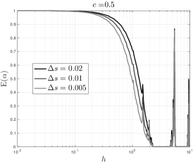
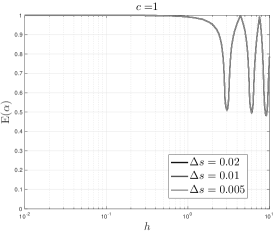
Figure 8.1: Ornstein-Uhlenbeck Bridge Example: Mean acceptance probability as a function of $h$ for the PRHMC algorithm for three choices of the splitting parameter $c$ and the three values of $\Delta s$. The number of time-steps $n$ at each integration leg is random with a geometric distribution chosen in such a way that the average length $\lambda=nh$ of the integration interval is 20. The number of samples is $10^{4}$. For $c=1$ the acceptance probability does not decrease as the grid is refined.

Remark 8.4.

Consider for a moment, a dynamics of the form (80) where $\boldsymbol{L}$ is an arbitrary negative-definite matrix and $\nabla G_{d}(\boldsymbol{u})$ is small with respect to $\boldsymbol{L}\boldsymbol{u}$. From a sampling viewpoint, this situation would arise if standard HMC is applied to sampling from a perturbation of the centered Gaussian distribution with covariance matrix $-\boldsymbol{L}^{-1}$. The preconditioning $\boldsymbol{M}=-\boldsymbol{L}$ makes sense in that setting. Large eigenvalues of $-\boldsymbol{L}$ correspond to directions in state space with small variances/large forces; the mass in those direction is then chosen to be large so as to ensure small displacements and avoid fast frequencies. This idea may be extended: general targets may be locally approximated by a state-dependent Gaussian model and one may then choose a state-dependent $M$ as the inverse of the covariance matrix of the Gaussian approximation (?). Unfortunately the state dependence of the mass matrix introduces additional terms in Hamilton’s equations, which are not any longer of the form (9), with the unwelcome consequence that explicit volume-preserving reversible integrators do not exist.

In the PHMC algorithm, the system (81) is integrated by means of a symplectic, reversible scheme with second order of accuracy. We use the Strang splitting (27) with

$$\begin{bmatrix}\boldsymbol{\dot{u}}(t)\\ \boldsymbol{\dot{p}}(t)\end{bmatrix}=\begin{bmatrix}-\boldsymbol{L}^{-1}\boldsymbol{p}(t)\\ c^{2}\boldsymbol{L}\boldsymbol{u}(t)\end{bmatrix}$$ (A)

and

$$\begin{bmatrix}\boldsymbol{\dot{u}}(t)\\ \boldsymbol{\dot{p}}(t)\end{bmatrix}=\begin{bmatrix}\boldsymbol{0}\\ (1-c^{2})\boldsymbol{L}\boldsymbol{u}(t)-\nabla G_{d}(\boldsymbol{u}(t))\end{bmatrix}$$ (B)

where $c\in[0,1]$ is a parameter. The choice $c=0$ leads to the velocity Verlet method.

Thus, in PHMC, a transition of the HMC Markov chain starts by drawing a fresh momentum from the marginal distribution $N(\boldsymbol{0},(\Delta s)^{-1}\boldsymbol{M})=N(\boldsymbol{0},-(\Delta s)^{-1}\boldsymbol{L})$, takes $m=\lfloor\lambda/h\rfloor$ steps of the splitting integrator and accepts/rejects with acceptance probability $\min\{1,e^{-\Delta\mathcal{H}_{d}}\}$ (see Algorithm 5.3). A variant, that we call PRMHC, with randomized duration as in Algorithm 5.5 is clearly possible; in that variant the number of steps is chosen to be geometrically distributed with mean $\lambda/h$.

Remark 8.5.

For implementation purposes, it is advisable to use the variable $\boldsymbol{v}=-\boldsymbol{L}^{-1}\boldsymbol{p}$ rather than $\boldsymbol{p}$. In the variables $(\boldsymbol{u},\boldsymbol{v})$, the split system (A) takes the trivial form $\boldsymbol{\dot{u}}(t)=\boldsymbol{v}(t)$, $\boldsymbol{\dot{v}}(t)=-c^{2}\boldsymbol{u}(t)$. Before beginning an integration leg, the fresh value of $\boldsymbol{v}$ is drawn from the corresponding distribution $N(\boldsymbol{0},(\Delta s)^{-1}\boldsymbol{L}^{-1})$. When computing the acceptance probability, the Hamiltonian $\mathcal{H}_{d}$ is correspondingly expressed in terms of $(\boldsymbol{u},\boldsymbol{v})$.

8.2.2 Numerical illustration

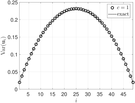
Figure 8.2: Ornstein-Uhlenbeck Bridge Example. This figure assesses the sampling accuracy of the PRHMC algorithm. The plot graphs, for the distribution $\Pi_{d}$, the exact and empirical values of the variance of $\boldsymbol{u}_{i}$ when $\Delta s=0.02$ corresponding to $d=49$ interior grid points (the horizontal axis labels the components). The time step size is $h=2.0$. The number of time-steps $n$ at each integration leg is random with a geometric distribution chosen in such a way that the average length $\lambda=nh$ of the integration interval is 20. The number of samples is $10^{6}$. The acceptance rate was $95\%$. When measured in the $L^{2}$ norm of $\mathbb{R}^{49}$, the relative error of the vector of empirical variances is $0.36\%$. The values $c=0$, $c=0.5$ were also tested but the acceptance rates were virtually zero.

We have implemented the randomized duration PRHMC algorithm in the particular case of the Orstein-Uhlenbeck bridge in Example 8.1, with $S=1$ and homogeneous Dirichlet boundary conditions (see Section 9.3 for the case of constant-duration PHMC). Note that due to the linearity of the Orstein-Uhlenbeck process, the target $\Pi_{d}$ is Gaussian and there is no need to use MCMC techniques to sample from it; however using this target provides a convenient test problem. Figure 8.1 plots the mean acceptance probability of PRHMC as a function of $h$ for three values of the parameter $c$ in the integrator and three choices of $\Delta s$. Clearly $c=1$ provides the best performance. Note in particular that for $c=1$ the acceptance probability is independent of $\Delta s$; for the other values of $c$ and fixed $h$ the acceptance probability decreases with $\Delta s$. Figure 8.2 shows that the use of $c=1$ leads to accurate sampling even with $h$ is large. The theory in what follows clarifies these numerical results.

8.2.3 Analysis

The results that follow are concerned with the application of PHMC and PRHMC to target associated with (75) in the particular case of the Orstein-Uhlenbeck bridge (77). The proofs are given in Section 9.4.

In the following stability theorem we require the lowest eigenvalue

$$\omega_{1}^{2}=\frac{4}{\Delta s^{2}}\sin^{2}\left(\frac{\pi}{2(d+1)}\right)$$ (82)

of $-\boldsymbol{L}$. It is trivial to show that $2/S\leq\omega_{1}$; therefore the stability requirements does not become more stringent as $\Delta s\rightarrow 0$. This is a consequence of the preconditioning of the dynamics.

Theorem 8.6.

If $h>0$ satisfies

$$\begin{cases}ch+2\arctan\left(\dfrac{h(1+(1-c^{2})\omega_{1}^{2})}{2c\omega_{1}^{2}}\right)<\pi&\text{if $c\in(0,1]$},\\ h<\dfrac{2\omega_{1}}{\sqrt{1+\omega_{1}^{2}}}&\text{if $c=0$},\end{cases}$$ (83)

then the splitting integrator used in the PHMC and PRMHC algorithms is stable.

We now turn to the mean energy error after an integration leg.

Theorem 8.7.

Choose $\eta\in(0,\pi)$ and restrict the attention to step sizes such that $ch\leq\eta$ and the stability requirement (83) is satisfied.

• For $c\in[0,1)$, there exist positive constants $h_{0}=h_{0}(c,\eta)$ and $C=C(c,\eta)$, such that for $h<h_{0}$, the mean energy error after $n$ time-steps has the bounds

  $$0\leq\mathbb{E}(\Delta\mathcal{H}_{d})\leq Cdh^{4}.$$

• In the case $c=1$, there exist positive constants $h_{0}=h_{0}(\eta)$ and $C^{\prime}=C^{\prime}(\eta)$, such that for $h<h_{0}$,

  $$0\leq\mathbb{E}(\Delta\mathcal{H}_{d})\leq C^{\prime}h^{4}.$$

Here, the expected value is over random initial conditions with non-normalized density $e^{-\mathcal{H}_{d}(\boldsymbol{u},\boldsymbol{p})}$.

The exponent of $h$ in the bounds should not be surprising by now. We emphasize that the bounds are independent of the number of steps in the integration leg. They therefore apply to the PHMC case where the duration of the integration leg is fixed and to cases where that duration is randomized as in the PRHMC algorithm in the experiments above. For $c\neq 1$ the energy error grows linearly with the number of degrees of freedom. This is the behaviour we found in the scenario studied in Section 7, but we note that here the different components $\boldsymbol{u}_{j}$ are not independent nor are they identically distributed (this point is discussed further in Section 9.4). On the other hand, for $c=1$ the energy error bound is uniform in $\Delta s$.

Even though full details will not be given, we mention that the bounds in Theorem 8.7 may be used to derive results on the acceptance rate, in analogy to what we did in Section 7. If $c=1$, the mean acceptance rate for fixed $h$ is independent of $\Delta s$. However for $c\neq 1$, $h$ has to be scaled as $(\Delta s)^{1/4}$ to ensure that the mean acceptance rate is bounded away from 0 as $\Delta s\rightarrow 0$. This agrees with the experiments in Figure 8.1. Note that the scaling $h\sim(\Delta s)^{1/4}$ arises from accuracy considerations rather than from stability restrictions.

8.3 Hilbert space HMC

The non-normalized density $\propto\exp(-\mathcal{U}_{d}(\boldsymbol{u}))$ of the target $\Pi_{d}$ associated with $\mathcal{U}_{d}(\boldsymbol{u})$ in (78) may be factored as

$$\exp(-\Delta sG_{d}(\boldsymbol{u}))\times\exp\Big{(}-\frac{\Delta s}{2}\boldsymbol{u}^{T}\boldsymbol{L}\boldsymbol{u}\Big{)}.$$ (84)

Thus $\Pi_{d}$ has non-normalized density

$$\exp(-\Delta sG_{d}(\boldsymbol{u}))$$ (85)

with respect to the Gaussian distribution $\Pi_{d}^{0}$ in $\mathbb{R}^{d}$ with mean $\boldsymbol{0}$ and covariance matrix $(\Delta s)^{-1}\boldsymbol{L}^{-1}$. This observation is useful because as $d\uparrow\infty$, $\Pi_{d}^{0}$ approaches the centered Gaussian distribution $\Pi^{0}$ in the Hilbert space $L^{2}(0,S)$ with covariance operator $(-\partial_{ss})^{-1}$, where the differential operator $-\partial_{ss}$ has homogeneous boundary conditions (?). It is well known that $\Pi^{0}$ is the distribution of the Brownian bridge in $[0,S]$ with homogeneous boundary conditions. On the other hand the first factor in (84) is a discretization of

$$\exp\left(-\int_{0}^{S}g(s,u(s))ds\right).$$

In this way the path distribution $\Pi$ may be described as the measure whose density with respect to the Gaussian $\Pi^{0}$ is given by the last display. There is an important difference between the finite and infinite dimensional cases. The finite dimensional $\Pi_{d}$ may described in two equivalent ways: (i) as having non-normalized density $\exp(-\mathcal{U}_{d}(\boldsymbol{u}))$ with respect to the standard Lebesgue measure $dq$ or (ii) as having non-normalized density (85) with respect to the Gaussian $\Pi_{d}^{0}$. The infinite-dimensional $\Pi$ cannot be defined by a density with respect to the standard Lebesgue measure in $L^{2}$, simply because that measure does not exist. Thus, necessarily $\Pi$ has to be defined by its density with respect to $\Pi^{0}$.

These considerations lead to studying the general problem of sampling from a target $\Pi$ defined by a density $\exp(-\Phi(u))$ with respect to a given centered Gaussian reference measure $\Pi_{0}$ in a Hilbert space. The PHMC and PRHMC algorithms described above in the restricted scenario of (75) may be extended without difficulty to that general problem. In the extension, the matrix $\boldsymbol{L}$ in (79) is replaced by a discretization of the inverse of the covariance operator of $\Pi_{0}$ and the function $G_{d}$ arises from discretizing $\Phi$. Again the key point in the preconditioned algorithms is to choose the mass matrix $\boldsymbol{M}$ to coincide with $-\boldsymbol{L}$; this ensures that if $\Phi=0$ the dynamics is given by $\boldsymbol{\ddot{u}}=-\boldsymbol{u}$ where all frequencies are $1$.

The general problem just described has been addressed by (?) who introduced an HMC algorithm that is formulated in the Hilbert space itself. Of course in practice that algorithm can only be implemented after a suitable discretization and, once the discretization has been performed, it coincides with PHMC with $c=1$ implemented as in Remark 8.5. We emphasize that in PHMC we first discretized the target and then formulated the sampling method. In contrast, (?) proceed in the reverse order: discretization comes after formulating the sampling method. The route in (?), which requires nontrivial use of functional analytic techniques, is mathematically more sophisticated than the approach we have followed here. What is then the advantage of formulating the algorithm in the infinite-dimensional scenario? A sampling method that works in the Hilbert space itself may be expected to work uniformly well as the dimension $d$ of the discretization tends to $\infty$. This is what happens to the algorithm in (?) in view of Theorem 8.7. On the other hand, for $c\neq 1$, PHMC cannot arise from discretizing a Hilbert space algorithm, because we know that its performance becomes worse and worse as $d\uparrow\infty$ with $h$ fixed.

To finish this section, we remark that for MALA preconditioned and non-preconditioned versions are available (?), and analogous to the latter, there is a non-preconditioned version of HMC (?).

9 Supplementary material

The paper concludes with material that complements a number of points considered in the preceding sections.

9.1 Finding the modified equation of a splitting integrator

We now show how to obtain the expansion in Theorem 4.3. Full details will be given for the particular case of the Lie-Trotter splitting algorithm (25); but the method is the same for more involved integrators. There are two steps. In the first, flows are represented as exponentials. In the second, exponentials are combined by means of the Baker-Campbell-Hausdorff (BCH) formula.

9.1.1 Lie derivatives

Associated with the vector field $f(x)$ in the differential system (1) with flow $\varphi_{t}$, there is a Lie derivative $D_{f}$. This is the first-order differential operator that maps each smooth function $\chi:\mathbb{R}^{D}\to\mathbb{R}$ into a new function $D_{f}\chi:\mathbb{R}^{D}\to\mathbb{R}$ defined as follows:

$$(D_{f}\chi)(x)=\sum_{i=1}^{D}f^{i}(x)\frac{\partial}{\partial x^{i}}\chi(x)$$

(superscripts denote components of vectors). The chain rule leads to the formula

$$\left.\frac{d}{dt}\chi\big{(}\varphi_{t}(x)\big{)}\right|_{t=0}=(D_{f}\chi)(x),$$

which shows the meaning of $(D_{f}\chi)(x)$ as a rate of change of $\chi$ along the solution $t\mapsto\varphi_{t}(x)$ of (1). By successively applying this formula to the functions $D_{f}\chi$, $D_{f}(D_{f}\chi)$, …, we find

$$\left.\frac{d^{k}}{dt^{k}}\chi\big{(}\varphi_{t}(x)\big{)}\right|_{t=0}=(D_{f}^{k}\chi)(x),\qquad k=2,3,\dots,$$

where $D^{k}_{f}$ is the $k$-th order differential operator defined inductively as

$$(D^{k}_{f}\chi)(x)=(D_{f}(D_{f}^{k-1}\chi))(x),\qquad k=2,3,\dots$$

Therefore the Taylor expansion of $\chi(\varphi_{t}(x))$ at $t=0$ reads

$$\chi\big{(}\varphi_{t}(x)\big{)}=\sum_{k=0}^{\infty}\frac{t^{k}}{k!}(D^{k}_{f}\chi)(x),$$

or

$$\chi\big{(}\varphi_{t}(x)\big{)}=\big{(}\exp(tD_{f})\chi\big{)}(x)$$

a formula that may be used to retrieve, at least formally, $\varphi_{t}$: its application with $\chi$ equal to the coordinate function $\chi(x)=x^{i}$, $i=1,\dots,D$, yields the $i$-th component of the vector $\varphi_{t}(x)$. In conclusion, the equality

$$\chi\circ\varphi_{t}=\exp(tD_{f})\chi$$ (86)

may be understood as a representation of the flow of a differential system as the exponential of the Lie operator of its vector field.

If $f^{(A)}$ and $f^{(B)}$ are vector fields, then the compositions $D_{f^{(A)}}D_{f^{(B)}}$ and $D_{f^{(B)}}D_{f^{(A)}}$ are second-order differential operators. However, it is easily checked that $D_{f^{(A)}}D_{f^{(B)}}-D_{f^{(B)}}D_{f^{{(A)}}}$ is a first-order differential operator. In fact the following result holds (?, Section 39).

Proposition 9.1.

$D_{f^{(A)}}D_{f^{(B)}}-D_{f^{(B)}}D_{f^{{(A)}}}$ is the Lie operator corresponding to the vector field $[f^{(A)},f^{(B)}]$ i.e. to the Lie bracket of $f^{(A)}$ and $f^{(B)}$ defined in (14).

If now $\varphi_{t}^{(A)}$, $\varphi_{s}^{(B)}$ are the flows corresponding to the vector fields $f^{(A)}$ and $f^{(B)}$ respectively, two applications of (86) give

$$\chi\circ\Big{(}\varphi_{s}^{{(B)}}\circ\varphi_{t}^{(A)}\Big{)} =\Big{(}\chi\circ\varphi_{s}^{{(B)}}\Big{)}\circ\varphi_{t}^{(A)}=\exp(tD_{f^{(A)}})\Big{(}\chi\circ\varphi_{s}^{{(B)}}\Big{)}$$ (87)

$$=\exp(tD_{f^{(A)}})\Big{(}\exp(sD_{f^{(B)}})\chi\Big{)}$$

$$=\Big{(}\exp(tD_{f^{(A)}})\exp(sD_{f^{(B)}})\Big{)}\chi.$$

Thus the operator $\exp(tD_{f^{(A)}})\exp(sD_{f^{(B)}})$ represents the composition $\varphi_{s}^{{(B)}}\circ\varphi_{t}^{(A)}$ in analogy with (86). Note that the $A$-flow acts first in the composition $\varphi_{s}^{{(B)}}\circ\varphi_{t}^{(A)}$ while $\exp(tD_{f^{(A)}})$ acts second in the product of operators $\exp(tD_{f^{(A)}})\exp(sD_{f^{(B)}})$. Our task now is to write $\exp(tD_{f^{(A)}})\exp(sD_{f^{(B)}})$ as a single exponential.

9.1.2 The Baker-Campbell-Hausdorff formula

Assume for the time being that $X$ and $Y$ are square matrices of the same dimension. It is well known that the product $\exp(X)\exp(Y)$ of their exponentials only coincides with $\exp(X+Y)$ if $X$ and $Y$ commute. In fact, by multiplying out

$$\exp(X)=I+X+\frac{1}{2}X^{2}+\frac{1}{6}X^{3}+\cdots$$

and

$$\exp(Y)=I+Y+\frac{1}{2}Y^{2}+\frac{1}{6}Y^{3}+\cdots$$

we find

$$\exp(X)\exp(Y) = I+X+Y+\frac{1}{2}X^{2}+XY+\frac{1}{2}Y^{2}$$

$$\frac{1}{6}X^{3}+\frac{1}{2}X^{2}Y+\frac{1}{2}XY^{2}+\frac{1}{6}X^{3}+\cdots$$

The products in the right-hand side are all of the form $X^{k}Y^{\ell}$, while the expansion of $\exp(X+Y)$ gives rise to products like $YX$, $Y^{2}X$, $YX^{2}$, $XYX$, $YXY$, etc. The BCH formula (?, ?) writes $\exp(X)\exp(Y)$ as the exponential $\exp(Z)$ of a matrix

$$Z = X+Y+\frac{1}{2}[X,Y]+\frac{1}{12}[X,[X,Y]]+\frac{1}{12}[Y,[Y,X]]$$

$$+\frac{1}{24}[X,[Y,[Y,X]]]-\frac{1}{720}[Y,[Y,[Y,[Y,X]]]]+\cdots$$

where $[\cdot,\cdot]$ denotes the commutator, e.g. $[X,Y]=XY-YX$, etc. The recipe to write down the terms in the right-hand side is of no consequence for our purposes; what is remarkable is that this right-hand side is a combination of $X$, $Y$ and iterated commutators.

Now the BCH is valid, at least formally (i.e. disregarding the convergence of the series involved), if $X$ and $Y$, instead of matrices, are elements of any associative, non-commutative algebra. In particular it may be applied to the case where $X$ and $Y$ are first-order differential operators as those considered above. Going back to (87) and recalling that the commutator of the Lie derivatives corresponds to the Lie bracket of the vector fields (Proposition 9.1), the BCH formula with $s=t=h$ then yields

$$\varphi_{h}^{{(B)}}\circ\varphi_{h}^{(A)}=\exp(hD_{\tilde{f}_{h}^{\infty}}),$$

where $f_{h}^{\infty}$ is the vector field

$$f_{h}^{\infty}=f^{(A)}+f^{(B)}+\frac{h}{2}[f^{(A)},f^{(B)}]+\frac{h^{2}}{12}[f^{(A)},[f^{(A)},f^{(B)}]]+\cdots$$

Now a comparison with (86) shows that $\varphi_{h}^{{(B)}}\circ\varphi_{h}^{(A)}$ is formally the $h$-flow of $f_{h}^{\infty}$, or, in other words, that $f_{h}^{\infty}$ is the modified vector-field for the Lie-Trotter splitting algorithm (25).

For Strang’s method and for more involved splitting integrators the methodology is the same: each of the individual flows whose composition yields $\psi_{h}$ is written as an exponential and then the exponentials are combined via the BCH formula. For an integrator where $\psi_{h}$ is the composition of $m$ flows, $m-1$ applications of the BCH are required. The task may be demanding due to the combinatorial intricacies of the BCH formula.

Remark 9.2.

As noted in Section 4, finding the modified vector field as above and then resorting to Theorem 4.4 is the most common way of investigating the consistency of splitting algorithms. An alternative direct technique, not based on modified equations, was suggested by (?). More recently, word series (?, ?) have been introduced as a simpler means to deal with this kind of question. A survey of the combinatorial techniques used to analyze integrators is provided by (?).

9.2 Distributions with light tails

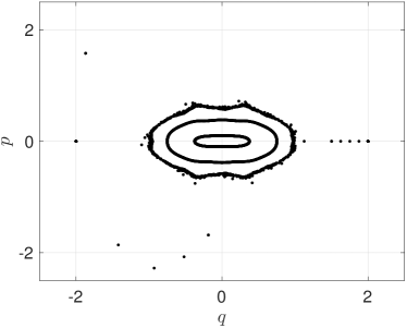
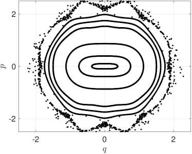
Figure 9.1: Verlet scheme for time step $h=1$ (left panel) and $h=1/2$ (right panel) applied to $H(q,p)=(1/2)p^{2}+(1/4)q^{4}$. The numerical solutions mimic the behaviour of the exact solution only for initial conditions close to the origin. Decreasing $h$ enlarges the region where the integrator performs satisfactorily, but does not eliminate the problem.

The numerical integration of Hamiltonian systems with a quadratic Hamiltonian (41) (which corresponds to HMC sampling of Gaussian distributions) was discussed in Section 3. For distributions whose tails are lighter than those of a Gaussian, the potential energy $\mathcal{U}(q)$ grows faster than quadratially as $|q|\rightarrow\infty$ and this causes difficulties when integrating numerically the Hamiltonian dynamics.

We illustrate this for the univariate distribution with non-normalized density $\exp(-q^{3})$. Figure 9.1 shows, for two values of $h$, nine velocity Verlet trajectories corresponding to initial conditions with $p=0$ and $q\in(0,2]$. While, for smaller values of the initial $q$ the numerical trajectory mimics the behaviour of the true solution, large initial values of $q$ lead to trajectories that quickly escape to infinity. Reducing the value of $h$ enlarges the size of the domain where Verlet performs satisfactorily. However no matter how small $h$ is chosen, there will be an outer region where the performance is bad. This is easily understood. The kicks of the Verlet algorithm update $p$ by using the formula $p\mapsto p-(h/2)q^{3}$. For this update to be a reasonable approximation to the true dynamics, it is obvious that the magnitude of $(h/2)q^{3}$ should be small when compared with the magnitude of $p$; a requirement that does not hold for any fixed $h$ and $p$ if $|q|$ is sufficiently large. The problem is the same for other explicit integrators. For implicit integrators, such as the midpoint rule, the solution of the algebraic equations to be solved at each step also demands smaller values of $h$ for larger values of $q$ as discussed in (?, Section 3.3.3).

The conclusion is that, when using an integrator with fixed $h$, one’s attention has to be restricted to a bounded subset $D$ of the phase space $\mathbb{R}^{2d}$ chosen to guarantee that the complement $\mathbb{R}^{2d}\backslash D$ has negligible probability with respect to $\Pi_{\operatorname{BG}}$. After fixing $D$, a suitably small value of $h$ has to be chosen. While the situation is well understood for the sampling algorithm MALA (?), the corresponding analysis for HMC has not yet been carried out.

9.3 Randomizing the time step and the duration

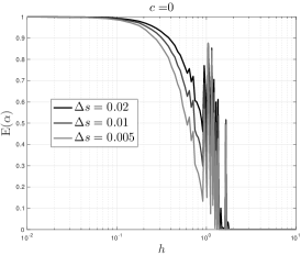
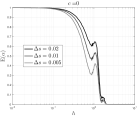
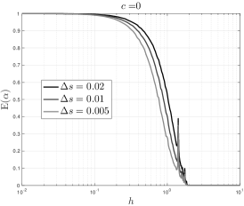
Figure 9.2: Time-Step or Duration Randomization. Ornstein-Uhlenbeck Bridge Example. Mean acceptance probability as a function of $h$ for PHMC operated with constant step sizes (first panel), PHMC operated with randomized step sizes of average $h$ (second panel), and PRHMC (third panel) for $c=0$ and three values of $\Delta s$. In all three cases the duration parameter is $\lambda=20$. The number of samples is $10^{4}$. The PRHMC algorithm is the least susceptible to periodicities in the underlying Hamiltonian dynamics.

The Exact RHMC algorithm, where the length of the integration leg is a random variable with exponential distribution was discussed at the end of Section 5, along with its numerical counterpart. We also discussed there an alternative procedure, based on randomizing the step length. We now illustrate the performance of these randomized algorithms in the case of the Ornstein-Uhlenbeck bridge example considered in Section 8. With the notation employed there, we set $c=0$, which leads to the standard Verlet integrator. We have implemented three algorithms: (i) PHMC operated with (constant) step sizes of length $h$, (ii) PHMC operated with step sizes of length $\Delta t$ uniformly distributed in the interval $[0.9h,1.1h]$ and (iii) PRHMC. The results are given in Figure 9.2. (The third panel here is the same as the first panel in Figure 8.1.) As $h$ varies, the behaviour of the un-randomized algorithm (i) is very irregular due to resonances between the step size and the periods of the dynamics (see Section 5.2). Randomizing $h$ regularizes the behaviour, but not as successfully as PRMHC does. This is consistent with the study carried out in §4 and §5 of (?).

The results of experiments with $c=0.5$ and $c=1$, not reported here, show the same patterns.

9.4 PHMC for the Orstein-Uhlenbeck bridge: proofs

We now prove Theorems  8.6 and 8.7.

9.4.1 One degree of freedom

We begin by studying the application of the integrator used in PHMC to a one-degree-of-freedom, linear analog of the dynamics in (81) given by the Hamiltonian function

$$H(q,p)=\frac{1}{2}\omega^{-2}p^{2}+\frac{1}{2}(\omega^{2}+1)q^{2}.$$

If $\omega\gg 1$ this corresponds to the motion of a particle with large mass $\omega^{2}$ attached to a stiff spring of constant $1+\omega^{2}$. The solutions are periodic with a frequency $1+1/\omega^{2}$ that decreases as $\omega$ increases.

The one-step propagation matrix (cf. (36)) is given explicitly by

$$\tilde{M}_{h,c}=\begin{bmatrix}\cos(ch)-\dfrac{h\tilde{\omega}^{2}}{2c\omega^{2}}\sin(ch)&\dfrac{\sin(ch)}{c\omega^{2}}\\[6.0pt] -h\tilde{\omega}^{2}\cos(ch)-\dfrac{4c^{2}\omega^{4}-h^{2}\tilde{\omega}^{4}}{4c\omega^{2}}\sin(ch)&\cos(ch)-\dfrac{h\tilde{\omega}^{2}}{2c\omega^{2}}\sin(ch)\end{bmatrix},$$

with $\tilde{\omega}^{2}=1+(1-c^{2})\omega^{2}$, if $c\in(0,1]$, or

$$\tilde{M}_{h,c}=\begin{bmatrix}1-\dfrac{h^{2}}{2\omega^{2}}(1+\omega^{2})&\dfrac{h}{\omega^{2}}\\[6.0pt] \dfrac{h(1+\omega^{2})(h^{2}-(4-h^{2})\omega^{2})}{4\omega^{2}}&1-\dfrac{h^{2}}{2\omega^{2}}(1+\omega^{2}),\end{bmatrix}$$

if $c=0$.

The following result is concerned with the stability of the integrator. Note that the stability restriction on $h$ weakens as $\omega$ gets larger.

Proposition 9.3.

If $\omega>0$, $c\in[0,1]$, and $h>0$ satisfies

$$\begin{cases}ch+2\arctan\left(\dfrac{h(1+(1-c^{2})\omega^{2})}{2c\omega^{2}}\right)<\pi&\text{if $c\in(0,1]$}\;,\\ h<\dfrac{2\omega}{\sqrt{1+\omega^{2}}}&\text{if $c=0$}\;,\end{cases}$$ (88)

then the splitting integrator is stable.

Proof 9.4.

Since the integrator is symplectic $\det(\tilde{M}_{h,c})=1$ and stability is ensured if the magnitude of the trace is $<2$. The case $c=0$ is trivial. For the case $c\in(0,1]$, by means of elementary trigonometric formulas we find

$$\frac{1}{2}\operatorname{trace}(\tilde{M}_{h,c})=\dfrac{\cos(ch+\arctan(\dfrac{h\tilde{\omega}^{2}}{2c\omega^{2}}))}{\cos(\arctan(\dfrac{h\tilde{\omega}^{2}}{2c\omega^{2}}))}.$$

As $h$ increases from 0, stability is lost when $h$ is such that the sum of the arguments in the cosine functions reaches $\pi$, so that the numerator and the denominator are opposite.

As in Section 4.4, for stable integrations, $\tilde{M}_{h,c}$ may be written in the form (49), with $\cos(\theta_{h})=\operatorname{trace}(\tilde{M}_{h,c})/2$ and

$$\chi_{h}=\begin{cases}\dfrac{\sin(ch)}{c\omega^{2}\sin(\theta_{h})}&\text{if $c\in(0,1]$}.\\ \dfrac{h}{\omega^{2}\sin(\theta_{h})}&\text{if $c=0$}.\end{cases}$$

For the error $\Delta$ in $H$ after an integration leg, by proceeding as in the proof of Proposition 6.7, we may show:

Proposition 9.5.

For any positive integer $n$, $\omega>0$, $c\in[0,1]$, $\beta>0$ and $h>0$ satisfying the stability requirement (88), the energy error after $n$ steps satisfies

$$\mathbb{E}(\Delta)=\beta^{-1}\sin^{2}(n\theta_{h})\rho(c,\omega,h),$$

where the expected value is over random initial conditions with non-normalized density $e^{-\beta H(q,p)}$ and

$$\rho(c,\omega,h)=\frac{1}{2}\left(\widehat{\chi}_{h}^{2}+\frac{1}{\widehat{\chi}_{h}^{2}}-2\right)=\frac{1}{2}\left(\widehat{\chi}_{h}-\frac{1}{\widehat{\chi}_{h}}\right)^{2}\geq 0$$

with

$$\widehat{\chi}_{h}^{2}=(\omega^{2}+\omega^{4})\chi_{h}^{2}.$$

Accordingly

$$0\leq\mathbb{E}(\Delta)\leq\rho(c,\omega,h).$$

Our next result gives a representation for $\rho$. The proof is a tedious exercise in algebra and will not be given.

Proposition 9.6.

For $\omega>0$, $c\in[0,1]$, and $h>0$ satisfying the stability requirement (88), we have

$$\rho(c,\omega,h)=\frac{1}{2}\frac{h^{4}r^{2}}{(1+\omega^{-2})(1+\omega^{-2}-h^{2}r)},$$ (89)

where $r$ is the function

$$r(c,\omega,h)=\frac{1}{4}(1-c^{2}+\omega^{-2})^{2}+c^{2}(1-c^{2}+\omega^{-2})R(ch),$$

with

$$R(ch)=\frac{1-ch\cot(ch)}{(ch)^{2}}.$$

The function $R(\zeta)$ has the finite limit $1/3$ as $\zeta\rightarrow 0$. If $c>0$, $R(ch)$ is positive and increases monotonically in the interval $0<ch<\pi$, with $R(ch)\uparrow\infty$ as $ch\uparrow\pi$. As a consequence, $r$ is an increasing function of $h\in(0,\pi)$; the term $1+\omega^{-2}-h^{2}r$ in (89) approaches $0$ as $h$ approaches the upper limit of the stability interval. The preceding propositions imply that the mean energy error has an $\mathcal{O}(h^{4})$ bound. By now this result is hardly a surprise, because we are dealing with an integrator of order $\nu=2$.

9.4.2 $d$ degrees of freedom

We now address the application of PHMC to the target associated with (75) when $g(u)=(1/2)u^{2}$. Theorems 8.6 and 8.7 are proved by using in $\mathbb{R}^{d}$ an orthonormal basis of eigenvectors of $-\boldsymbol{L}$ (cf. the proof of (69)). In the basis of eigenvectors the different components are stochastically independent but not identically distributed.

For Theorem 8.6 it is enough to recall that in Proposition 9.3 larger values of $\omega$ lead to less stringent stability requirements. Therefore stability is limited by the smallest eigenvalue of $-\boldsymbol{L}$ given in (82).

Turning to the proof of Theorem 8.7, by using the spectral decomposition and Proposition 9.5 with $\beta=\Delta s$, we may write

$$0\leq\mathbb{E}(\Delta\mathcal{H}_{d})\leq\sum_{j=1}^{d}\rho(c,\omega_{j},h),$$

with $\omega_{j}^{2}$ equal to the $j$-th eigenvalue of $-\boldsymbol{L}$

$$\omega_{j}^{2}=\frac{4}{\Delta s^{2}}\sin^{2}\left(\frac{j\pi}{2(d+1)}\right)\geq\frac{4j^{2}}{S^{2}}.$$

We now use (89) to obtain the bound

$$0\leq\mathbb{E}(\Delta\mathcal{H}_{d})\leq\frac{h^{4}}{2}\sum_{j=1}^{d}\frac{r(c,\omega_{j},h)^{2}}{1-h^{2}r(c,\omega_{j},h)},$$

and, since $r$ is a decreasing function of $\omega$,

$$0\leq\mathbb{E}(\Delta\mathcal{H}_{d})\leq d\frac{h^{4}}{2}\frac{r(c,\omega_{1},h)^{2}}{1-h^{2}r(c,\omega_{1},h)}.$$

The first bound in the theorem now follows easily: for $h$ bounded away from $\pi$, $r$ is bounded, and then $h$ may be reduced further to ensure that $1-h^{2}r(c,\omega_{1},h)$ is bounded away from 0.

When $c=1$,

$$r(1,\omega_{j},h)=\frac{1}{4}\omega_{j}^{-4}+\omega_{j}^{-2}R(h)\leq\frac{S^{4}}{64j^{4}}+\frac{S^{2}}{4j^{2}}R(h),$$

and therefore for $h$ bounded away from $\pi$, $r(1,\omega_{j},h)=\mathcal{O}(j^{-2})$. Thus, if we write,

$$0\leq\mathbb{E}(\Delta\mathcal{H}_{d})\leq\frac{h^{4}}{2}\sum_{j=1}^{d}\frac{r(1,\omega_{j},h)^{2}}{1-h^{2}r(1,\omega_{1},h)},$$

the sum in the right-hand side may be bounded independently of $d$.

9.5 Convergence

Here is a brief discussion of the sampling properties of HMC.

Intuitively speaking, the point of using HMC is that its Hamiltonian dynamics breaks the random walk behaviour that impairs the convergence of simple MCMC methods like the random walk Metropolis or the MALA algorithm (?, ?). This slow convergence can be understood by using a diffusion approximation of these simple MCMC methods. In particular, the processes associated to simple MCMC methods are often well approximated (in a weak sense) by overdamped Langevin dynamics (?, see Theorem 5.1 for a precise mathematical statement), also called Brownian dynamics. This may be seen as a consequence of the detailed balance property of the algorithms. As a result, the corresponding paths meander around state space and explore the target distribution mainly by diffusion. Qualitatively speaking, this is random walk behavior. The basic idea in HMC is to replace the first-order Langevin dynamics in order to avoid this random walk behaviour.

Unfortunately, beyond this intuition, the improvement in convergence afforded by HMC is not well understood. Under certain conditions on the time-step and target distribution, it has been known for a while that numerical HMC converges to the right distribution asymptotically (?, ?, ?). More recently, the piecewise deterministic process associated with the exact RHMC Algorithm 5.4 was shown to be geometrically ergodic; i.e., its transition probabilities converge to the target distribution in the total variation metric at an exponential rate (?, see Theorem 3.9). The proof of geometric ergodicity of RHMC relies on Harris theorem, which requires a (local) version of Doeblin’s condition: a minorization condition for the transition probabilities at a finite time and in a compact set. Unfortunately, given the complicated form of these transition probabilities, the minorization condition involves non-explicit constants, and in particular, the dependence of the resulting convergence rate on the mean duration parameter is not clear.

Using a coupling approach, a contraction rate for exact RHMC in a Wasserstein distance has been derived (?). The dependence of the contraction rate on the mean duration parameter is explicit. It follows from this rate that, if the mean duration parameter is proportional to the standard deviation of the target distribution, then the algorithm converges at a kinetic speed (as opposed to a diffusive speed). The main tools used in the proof are a Markovian coupling and a coupling distance that are both tailored to the structure of exact RHMC. The coupling is based on the framework introduced in (?), and is related to a recently developed coupling for second-order Langevin dynamics (?, ?).

9.6 Related Algorithms

We finally discuss generalizations and variants of the basic HMC Algorithm 5.3. The corresponding literature is extensive and rapidly growing; we limit ourselves to a few of the many available techniques.

9.6.1 Generalized HMC

Generalized HMC (GHMC) allows the possibility of partial randomization of momentum at every step of the HMC algorithm (?, ?). Specifically, in GHMC, one introduces a so-called Horowitz angle $\phi\in(0,\pi/2]$ and replaces the randomized momentum $\xi_{0}$ in Step 1 of Algorithm 5.3 with $\cos(\phi)p_{0}+\sin(\phi)\xi_{0}$. This partial momentum randomization preserves the $p$-marginal of $\Pi_{\operatorname{BG}}$, and hence, GHMC leaves $\Pi_{\operatorname{BG}}$ invariant. When $\phi=\pi/2$, the initial momentum $p_{0}$ is fully randomized and we recover HMC. If $\phi\in(0,\pi/2)$, then $p_{0}$ is only partially randomized; this may be of interest in molecular dynamics applications because then the samples may give more information on the Hamiltonian dynamics than when each integration leg starts with a completely new momentum. The case $\phi=0$ is excluded, since then there is no momentum randomization, and consequently, the GHMC chain is confined to a single level set of $H$, and in general, is not ergodic with respect to $\Pi_{\operatorname{BG}}$. Since the momentum randomizations are the source of dissipation in HMC (?), partial momentum randomization makes the algorithm less dissipative and less diffusive, as discussed in §5.5.3 of (?). One can similarly introduce a partial momentum randomization to the randomized HMC Algorithm 5.5.

9.6.2 Extra Chance HMC

As we pointed out before, rejections increase correlations along the HMC chain and waste computational effort. Extra chance HMC (XHMC) (?) provides a simple way for HMC to get extra chances to obtain acceptance, and hence, delay or even avert rejection as in (?, ?). To describe the XHMC algorithm, it suffices to describe its accept/reject mechanism, which we state in terms of a symplectic and reversible integrator $\psi_{h}$, and its $n$-step map, $\Psi_{\lambda}=\psi_{h}^{n}$ where $n=\lfloor\lambda/h\rfloor$. Given a user-prescribed number of extra chances $K$ and $(q,p)\in\mathbb{R}^{2d}$, define $\Gamma^{0}(q,p)=0$, $\Gamma^{K+1}(q,p)=1$, and

$$\Gamma^{j}(q,p)=\alpha(q,p)\vee\cdots\vee\alpha^{j}(q,p)\;,\qquad 1\leq j\leq K\;,$$

where $\alpha^{j}(q,p)=\min\left\{1,e^{-\left(H(\Psi_{\lambda}^{j}(q,p))-H(q,p)\right)}\right\}$. Note that $\Gamma^{j}$ is monotonically increasing with $j$. Instead of flipping a coin at every step as in Algorithm 5.3, XHMC rolls a $(K+1)$-sided die with probabilities $\{\Gamma^{j}-\Gamma^{j-1}\}_{j=1}^{K+1}$. Given the current state of the chain $(q_{0},p_{0})\in\mathbb{R}^{2d}$, the transition in Step 3 of Algorithm 5.3 is accordingly replaced by

$$(q_{1},p_{1})=\begin{cases}\Psi_{\lambda}^{j}(q_{0},\xi_{0})&\text{if $j$-th side of die comes up}\\ (q_{0},-\xi_{0})&\text{if $(K+1)$-th side of die comes up}\end{cases}$$

where $\xi_{0}\sim\mathcal{N}(0,M)$. It is straightforward to show that XHMC leaves $\Pi_{\operatorname{BG}}$ invariant (?, Appendix A). Moreover, thanks to the possibility of extra chances, the probability of rejection at every step drops from $\alpha(q_{0},p_{0})$ to $1-\Gamma^{K}(q_{0},p_{0})$. As its name suggests, the accept/reject mechanism in XHMC can be implemented recursively, so that the proposal move $\Psi_{\lambda}^{j}(q_{0},p_{0})$ and its associated transition probability $\Gamma^{j}-\Gamma^{j-1}$ are only computed if $\Psi_{\lambda}^{j-1}(q_{0},p_{0})$ is not accepted. One can also easily incorporate a partial momentum randomization into XHMC.

9.6.3 Tempering techniques

Probability distributions with multiple modes arise frequently in practice. Different modes may represent metastable conformations of a large molecular system (?, ?, ?, ?, ?) or important features of posterior distributions in Bayesian inference problems (?, ?, ?, ?, ?). Unfortunately, HMC may not converge well in situations where the potential energy has multiple minima separated by large barriers. This is a well-known limitation of HMC. It may be due to the low probability of the momentum randomizations in HMC to produce an initial condition whose kinetic energy is high enough so that the corresponding solution to Hamilton’s equations crosses the potential energy barriers. Also the momentum randomization may have difficulties to produce an initial momentum $\xi_{0}$ with the right direction for the solution to Hamilton’s equation to exit the current potential well. For such multi-modal target distributions, it is advantageous to use HMC in conjunction with a tempering technique such as parallel tempering, simulated tempering, and tempered transition methods (?, ?, ?, ?). Tempering methods typically introduce an artificial inverse temperature parameter $\beta$ and apply HMC to the Boltzmann-Gibbs distribution at multiple values of this parameter. The basic idea is that at sufficiently high temperature, the tempered Boltzmann-Gibbs distribution becomes flat enough that barrier crossings in the Hamiltonian integration legs become more likely. Of course, the states of the tempered chains cannot be directly used to compute sample averages with respect to $\Pi_{\operatorname{BG}}$, which emphasizes that the computational cost of these tempering techniques is by no means negligible.

9.6.4 No-U-Turns

A practical difficulty with HMC is tuning the durations of the Hamiltonian integration legs. The No-U-Turn Sampler (NUTS) adaptively chooses this parameter by increasing the length of the numerical orbit until the distance between the endpoints of the orbit stops increasing. Unfortunately, this procedure breaks reversibility, since, roughly speaking, if this criterion is applied in the reverse direction starting from the end of a trajectory, one does not expect to land at the start of the trajectory. Since reversibility is a key ingredient to the accept/reject mechanism in Algorithm 5.1, and the proof of the associated Theorem 5.5, NUTS uses a different approach: it applies the criterion to the discrete trajectory obtained by integrating the Hamiltonian dynamics in the forward and backward directions. Starting with a single step, the number of forward and backward integration steps is doubled until a U-turn first occurs. NUTS then ends the simulation and samples from all of these points in a way that ensures that the algorithm leaves $\Pi_{\operatorname{BG}}$ invariant. The procedure does not use the Metropolis-Hastings method, but a variant of the slice sampling method (?). Since this sampling step involves all of the states produced by this procedure, the algorithm is thought to have some of the appealing properties of the windowed HMC method, which employs an accept/reject mechanism based on windows of states (?, ?).

9.6.5 Shadow HMC

Given a symplectic and reversible integrator $\psi_{h}$ for the Hamiltonian dynamics, shadow HMC is an importance sampling technique that replaces the Boltzmann-Gibbs density $\exp(-H)$ with a shadow density $\exp(-\tilde{H}_{h}^{[\mu]})$ where $\tilde{H}_{h}^{[\mu]}$ is the modified (or shadow) Hamiltonian of $\psi_{h}$ up to order $\mu$ (?, ?, ?). In so doing, shadow HMC samples from a different target density and the samples have to be reweighed in order to compute averages with respect to the target distribution. This method is not to be confused with the so-called surrogate transition method (?), since in shadow HMC the target density is altered. The rationale for shadow HMC is that $\exp(-\tilde{H}_{h})$ is easy to sample from, in the sense that $\psi_{h}$ preserves $\tilde{H}_{h}$ much more accurately than $H$, and hence, for a given duration parameter, shadow HMC increases the acceptance probability without having to reduce the time step $h$. There is also a shadow generalized HMC method, which similarly replaces the target density in GHMC with $\exp(-\tilde{H}_{h})$. Several aspects of shadow HMC have not been sufficiently analyzed from a mathematical viewpoint. For instance the integrability of $\exp(-\tilde{H}_{h}^{[\mu]})$ has not been studied in depth. Moreover, shadow HMC requires estimating the modified Hamiltonian to order $\mu$, which is nontrivial since it requires computing (or estimating) higher derivatives of $\mathcal{U}$ (?). The momentum randomization step in Algorithm 5.3 must be modified, since the $p$-marginal of $\exp(-\tilde{H}_{h}^{[\mu]})$ is no longer a Gaussian distribution.

References

- [1]
- [2] [] E. Akhmatskaya and S. Reich (2008), ‘GSHMC: An efficient method for molecular simulation’, J. Comput. Phys. 227, 4937–4954.
- [3]
- [4] [] E. Akhmatskaya, M. Fernández-Pendás, T. Radivojević and J. M. Sanz-Serna (2017), Adaptive splitting integrators for enhancing sampling efficiency of modified Hamiltonian Mnte Carlo methods in molecular simulation, to appear in Langmuir.
- [5]
- [6] [] A. Alamo and J. M. Sanz-Serna (2016), ‘A technique for studying strong and weak local errors of splitting stochastic integrators’, SIAM J. Numer. Anal. 54(6), 3239–3257.
- [7]
- [8] [] M. P. Allen and D. J. Tildesley (1987), Computer Simulation of Liquids, Clarendon Press.
- [9]
- [10] [] C. Andrieu, N. De Freitas, A. Doucet and M. I. Jordan (2003), ‘An introduction to MCMC for machine learning’, Machine learning 50(1-2), 5–43.
- [11]
- [12] [] V. I. Arnol’d (1989), Mathematical methods of classical mechanics, Vol. 60 of Graduate Texts in Mathematics, Springer-Verlag, New York. Translated from the 1974 Russian original by K. Vogtmann and A. Weinstein, Corrected reprint of the second (1989) edition.
- [13]
- [14] [] S. Asmussen and P. W. Glynn (2007), Stochastic simulation: Algorithms and analysis, Vol. 57, Springer Science & Business Media.
- [15]
- [16] [] A. Beskos, N. S. Pillai, G. O. Roberts, J. M. Sanz-Serna and A. M. Stuart (2013), ‘Optimal tuning of hybrid Monte-Carlo algorithm’, Bernoulli 19, 1501–1534.
- [17]
- [18] [] A. Beskos, F. J. Pinski, J. M. Sanz-Serna and A. M. Stuart (2011), ‘Hybrid Monte-Carlo on Hilbert spaces’, Stochastic Processes and their Applications 121(10), 2201–2230.
- [19]
- [20] [] A. Beskos, G. Roberts, A. Stuart and J. Voss (2008), ‘MCMC methods for diffusion bridges’, Stochastics and Dynamics 8(03), 319–350.
- [21]
- [22] [] C. M. Bishop (2006), Pattern recognition and machine learning, springer.
- [23]
- [24] [] S. Blanes and F. Casas (2016), A concise introduction to geometric numerical integration, Monographs and Research Notes in Mathematics, CRC Press, Boca Raton.
- [25]
- [26] [] S. Blanes, F. Casas and J. M. Sanz-Serna (2014), ‘Numerical integrators for the hybrid Monte Carlo method’, SIAM Journal on Scientific Computing 36(4), A1556–A1580.
- [27]
- [28] [] N. Bou-Rabee (2014), ‘Time integrators for molecular dynamics’, Entropy 16, 138–162.
- [29]
- [30] [] N. Bou-Rabee (2017), ‘Cayley splitting for second-order langevin stochastic partial differential equations’, arXiv preprint arXiv:1707.05603.
- [31]
- [32] [] N. Bou-Rabee and A. Eberle (2017), Coupling and convergence for exact randomized Hamiltonian Monte-Carlo.
- [33]
- [34] [] N. Bou-Rabee and M. Hairer (2013), ‘Non-asymptotic mixing of the MALA algorithm’, IMA J. Numer. Anal. 33, 80–110.
- [35]
- [36] [] N. Bou-Rabee and J. M. Sanz-Serna (2017), ‘Randomized Hamiltonian Monte Carlo’, Ann Appl Probab 27(4), 2159 – 2194.
- [37]
- [38] [] N. Bou-Rabee and E. Vanden-Eijnden (2010), ‘Pathwise accuracy and ergodicity of Metropolized integrators for SDEs’, Comm. Pure and Appl. Math. 63, 655–696.
- [39]
- [40] [] N. Bou-Rabee and E. Vanden-Eijnden (2012), ‘A patch that imparts unconditional stability to explicit integrators for Langevin-like equations’, J Comput Phys 231, 2565–2580.
- [41]
- [42] [] N. Bou-Rabee, A. Donev and E. Vanden-Eijnden (2014), ‘Metropolis integration schemes for self-adjoint diffusions’, Multiscale Modeling & Simulation 12, 781–831.
- [43]
- [44] [] J. C. Butcher (2016), Numerical methods for ordinary differential equations, third edn, John Wiley & Sons, Ltd., Chichester. With a foreword by J. M. Sanz-Serna.
- [45]
- [46] [] M. P. Calvo and J. M. Sanz-Serna (1993), ‘The development of variable-step symplectic integrators, with application to the two-body problem’, SIAM J. Sci. Comput. 14(4), 936–952.
- [47]
- [48] [] M. P. Calvo and J. M. Sanz-Serna (2009), ‘Instabilities and inaccuracies in the integration of highly oscillatory problems’, SIAM J. Sci. Comput. 31(3), 1653–1677.
- [49]
- [50] [] M. P. Calvo, A. Murua and J. M. Sanz-Serna (1994), Modified equations for ODEs, in Chaotic numerics (Geelong, 1993), Vol. 172 of Contemp. Math., Amer. Math. Soc., Providence, RI, pp. 63–74.
- [51]
- [52] [] C. M. Campos and J. M. Sanz-Serna (2015), ‘Extra chance generalized hybrid Monte Carlo’, J. Comput. Phys. 281, 365–374.
- [53]
- [54] [] C. M. Campos and J. M. Sanz-Serna (2017), ‘Palindromic 3-stage splitting integrators, a roadmap’, J. Comput. Phys. 346, 340–355.
- [55]
- [56] [] E. Cancés, F. Legoll and G. Stoltz (2007), ‘Theoretical and numerical comparison of some sampling methods for molecular dynamics’, Mathematical Modelling and Numerical Analysis 41, 351–389.
- [57]
- [58] [] B. Cano and J. M. Sanz-Serna (1997), ‘Error growth in the numerical integration of periodic orbits, with application to Hamiltonian and reversible systems’, SIAM J. Numer. Anal. 34(4), 1391–1417.
- [59]
- [60] [] B. Cano and J. M. Sanz-Serna (1998), ‘Error growth in the numerical integration of periodic orbits by multistep methods, with application to reversible systems’, IMA J. Numer. Anal. 18(1), 57–75.
- [61]
- [62] [] B. Carpenter, A. Gelman, M. Hoffman, D. Lee, B. Goodrich, M. Betancourt, M. A. Brubaker, J. Guo, P. Li and A. Riddell (2016), ‘Stan: A probabilistic programming language’, Journal of Statistical Software 20, 1–37.
- [63]
- [64] [] Z. Chen (2003), ‘Bayesian filtering: From Kalman filters to particle filters, and beyond’, Statistics 182(1), 1–69.
- [65]
- [66] [] B. A. Cipra (2000), ‘The best of the 20th century: Editors name top 10 algorithms’, SIAM News.
- [67]
- [68] [] G. Da Prato and J. Zabczyk (2014), Stochastic equations in infinite dimensions, Cambridge university press.
- [69]
- [70] [] P. Diaconis (2009), ‘The Markov Chain Monte Carlo revolution’, Bulletin of the American Mathematical Society 46(2), 179–205.
- [71]
- [72] [] P. Diaconis, S. Holmes and R. M. Neal (2000), ‘Analysis of a nonreversible markov chain sampler’, Annals of Applied Probability pp. 726–752.
- [73]
- [74] [] S. Duane, A. D. Kennedy, B. J. Pendleton and D. Roweth (1987), ‘Hybrid Monte-Carlo’, Phys Lett B 195, 216–222.
- [75]
- [76] [] A. Eberle (2016a), A coupling approach to the kinetic Langevin equation on the torus.
- [77]
- [78] [] A. Eberle (2016b), ‘Reflection couplings and contraction rates for diffusions’, Probability theory and related fields 166(3-4), 851–886.
- [79]
- [80] [] A. Eberle, A. Guillin and R. Zimmer (2016), Couplings and quantitative contraction rates for Langevin dynamics.
- [81]
- [82] [] G. Evensen (2009), Data assimilation: the ensemble Kalman filter, Springer Science & Business Media.
- [83]
- [84] [] Y. Fang, J. M. Sanz-Serna and R. D. Skeel (2014), ‘Compressible generalized hybrid Monte Carlo’, The Journal of chemical physics 140(17), 174108.
- [85]
- [86] [] M. Fathi (2014), Theoretical and numerical study of a few stochastic models of statistical physics, PhD thesis, Université Pierre et Marie Curie-Paris VI.
- [87]
- [88] [] M. Fathi, A.-A. Homman and G. Stoltz (2015), ‘Error analysis of the transport properties of Metropolized schemes’, ESAIM: Proceedings and Surveys 48, 341–363.
- [89]
- [90] [] K. Feng and M. Qin (2010), Symplectic geometric algorithms for Hamiltonian systems, Zhejiang Science and Technology Publishing House, Hangzhou; Springer, Heidelberg. Translated and revised from the Chinese original, With a foreword by Feng Duan.
- [91]
- [92] [] M. Fernández-Pendás, E. Akhmatskaya and J. M. Sanz-Serna (2016), ‘Adaptive multi-stage integrators for optimal energy conservation in molecular simulations’, J. Comput. Phys. 327, 434–449.
- [93]
- [94] [] D. D. Frantz, D. L. Freeman and J. D. Doll (1990), ‘Reducing quasi-ergodic behavior in monte carlo simulations by j-walking: Applications to atomic clusters’, Journal of Chemical Physics 93(4), 2769–2784.
- [95]
- [96] [] D. Frenkel and B. Smit (2002), Understanding Molecular Simulation: From algorithms to Applications, Second Edition, Academic Press.
- [97]
- [98] [] A. E. Gelfand and A. F. M. Smith (1990), ‘Sampling-based approaches to calculating marginal densities’, Journal of the American statistical association 85(410), 398–409.
- [99]
- [100] [] S. Geman and D. Geman (1984), ‘Stochastic relaxation, Gibbs distributions, and the Bayesian restoration of images’, IEEE Transactions on pattern analysis and machine intelligence (6), 721–741.
- [101]
- [102] [] C. J. Geyer (1991), ‘Markov Chain Monte Carlo maximum likelihood’.
- [103]
- [104] [] C. J. Geyer (1992), ‘Practical Markov Chain Monte Carlo’, Statistical science pp. 473–483.
- [105]
- [106] [] C. J. Geyer and E. A. Thompson (1995), ‘Annealing markov chain monte carlo with applications to ancestral inference’, Journal of the American Statistical Association 90(431), 909–920.
- [107]
- [108] [] Z. Ghahramani (2015), ‘Probabilistic machine learning and artificial intelligence’, Nature 521(7553), 452.
- [109]
- [110] [] M. Girolami and B. Calderhead (2011), ‘Riemann manifold Langevin and Hamiltonian Monte Carlo methods’, J R Statist Soc B 73, 123–214.
- [111]
- [112] [] P. J. Green and A. Mira (2001), ‘Delayed rejection in reversible jump Metropolis–Hastings’, Biometrika 88(4), 1035–1053.
- [113]
- [114] [] D. F. Griffiths and D. J. Higham (2010), Numerical methods for ordinary differential equations, Springer Undergraduate Mathematics Series, Springer-Verlag London, Ltd., London. Initial value problems.
- [115]
- [116] [] D. F. Griffiths and J. M. Sanz-Serna (1986), ‘On the scope of the method of modified equations’, SIAM J. Sci. Statist. Comput. 7(3), 994–1008.
- [117]
- [118] [] P. Gustafson (1998), ‘A guided walk Metropolis algorithm’, Statistics and Computing 8(4), 357–364.
- [119]
- [120] [] J. D. Hadfield (2010), ‘MCMC methods for multi-response generalized linear mixed models: the MCMCglmm R package’, Journal of Statistical Software 33(2), 1–22.
- [121]
- [122] [] E. Hairer and G. Wanner (2010), Solving ordinary differential equations. II, Vol. 14 of Springer Series in Computational Mathematics, Springer-Verlag, Berlin. Stiff and differential-algebraic problems, Second revised edition, paperback.
- [123]
- [124] [] E. Hairer, C. Lubich and G. Wanner (2010), Geometric Numerical Integration, Springer.
- [125]
- [126] [] E. Hairer, S. P. Nørsett and G. Wanner (1993), Solving Ordinary Differential Equations I, Springer-Verlag.
- [127]
- [128] [] M. Hairer, A. M. Stuart and J. Voss (2009), ‘Sampling conditioned diffusions’, Trends in stochastic analysis 353, 159–186.
- [129]
- [130] [] U. H. E. Hansmann (1997), ‘Parallel tempering algorithm for conformational studies of biological molecules’, Chemical Physics Letters 281(1), 140–150.
- [131]
- [132] [] U. H. E. Hansmann and Y. Okamoto (1993), ‘Prediction of peptide conformation by multicanonical algorithm: New approach to the multiple-minima problem’, J Comput Chem 14(11), 1333–1338.
- [133]
- [134] [] W. K. Hastings (1970), ‘Monte-Carlo methods using Markov chains and their applications’, Biometrika 57, 97–109.
- [135]
- [136] [] B. Hess, C. Kutzner, D. van der Spoel and D. Lindahl (2008), ‘Gromacs 4: Algorithms for highly efficient, load-balanced, and scalable molecular simulation’, J. Chem. Theory Comp. 4, 435—447.
- [137]
- [138] [] M. D. Homan and A. Gelman (2014), ‘The no-u-turn sampler: Adaptively setting path lengths in hamiltonian monte carlo’, The Journal of Machine Learning Research 15(1), 1593–1623.
- [139]
- [140] [] A. M. Horowitz (1991), ‘A generalized guided Monte-Carlo algorithm’, Phys Lett B 268, 247–252.
- [141]
- [142] [] A. Iserles and G. R. W. Quispel (2017), Why geometric integration.
- [143]
- [144] [] J. A. Izaguirre and S. S. Hampton (2004), ‘Shadow hybrid Monte Carlo: an efficient propagator in phase space of macromolecules’, J Comp Phys 200(2), 581–604.
- [145]
- [146] [] S. T. Jensen, X. S. Liu, Q. Zhou and J. S. Liu (2004), ‘Computational discovery of gene regulatory binding motifs: a Bayesian perspective’, Statistical Science pp. 188–204.
- [147]
- [148] [] H. Ji and W. H. Wong (2006), ‘Computational biology: toward deciphering gene regulatory information in mammalian genomes’, Biometrics 62(3), 645–663.
- [149]
- [150] [] A. D. Kennedy and B. Pendleton (2001), ‘Cost of the generalized hybrid Monte Carlo algorithm for free field theory’, Nucl Phys B 607, 456–510.
- [151]
- [152] [] K. Kikuchi, M. Yoshida, T. Maekawa and H. Watanabe (1991), ‘Metropolis monte carlo method as a numerical technique to solve the fokker-planck equation’, Chem Phys Lett 185, 335–338.
- [153]
- [154] [] S. C. Kou, Q. Zhou and W. H. Wong (2006), ‘Discussion paper equi-energy sampler with applications in statistical inference and statistical mechanics’, Annals of Statistics pp. 1581–1619.
- [155]
- [156] [] W. Krauth (2006), Statistical mechanics: algorithms and computations, Vol. 13, OUP Oxford.
- [157]
- [158] [] J. S. W. Lamb and J. A. G. Roberts (1998), ‘Time-reversal symmetry in dynamical systems: a survey’, Physica D: Nonlinear Phenomena 112(1), 1–39.
- [159]
- [160] [] D. P. Landau and K. Binder (2014), A guide to Monte Carlo simulations in statistical physics, Cambridge university press.
- [161]
- [162] [] B. Leimkuhler and S. Reich (2004), Simulating Hamiltonian Dynamics, Cambridge Monographs on Applied and Computational Mathematics, Cambridge University Press.
- [163]
- [164] [] T. Lelievre, M. Rousset and G. Stoltz (2010), Free energy computations: A mathematical perspective, Imperial College Press.
- [165]
- [166] [] F. Liang and W. H. Wong (2001), ‘Real-parameter evolutionary monte carlo with applications to bayesian mixture models’, Journal of the American Statistical Association 96(454), 653–666.
- [167]
- [168] [] W. A. Link and R. J. Barker (2009), Bayesian inference: with ecological applications, Academic Press.
- [169]
- [170] [] J. S. Liu (2008), Monte Carlo Strategies in Scientific Computing, 2nd edn, Springer.
- [171]
- [172] [] D. J. Lunn, A. Thomas, N. Best and D. Spiegelhalter (2000), ‘WinBUGS-a Bayesian modelling framework: concepts, structure, and extensibility’, Statistics and computing 10(4), 325–337.
- [173]
- [174] [] D. Lunn, C. Jackson, N. Best, A. Thomas and D. Spiegelhalter (2012), The BUGS book: A practical introduction to Bayesian analysis, CRC press.
- [175]
- [176] [] D. Lunn, D. Spiegelhalter, A. Thomas and N. Best (2009), ‘The BUGS project: evolution, critique and future directions’, Statistics in medicine 28(25), 3049–3067.
- [177]
- [178] [] P. B. Mackenzie (1989), ‘An improved hybrid Monte Carlo method’, Physics Letters B 226(3), 369–371.
- [179]
- [180] [] J. Mannseth, T. S. Kleppe and H. J. Skaug (2017), On the application of improved symplectic integrators in hamiltonian monte carlo, Communications in Statistics - Simulation and Computation, to appear.
- [181]
- [182] [] E. Marinari and G. Parisi (1992), ‘Simulated tempering: a new monte carlo scheme’, EPL (Europhysics Letters) 19(6), 451.
- [183]
- [184] [] J. Marsden and T. Ratiu (1999), Introduction to Mechanics and Symmetry, Springer Texts in Applied Mathematics.
- [185]
- [186] [] A. D. Martin, K. M. Quinn and J. H. Park (2011), ‘MCMCpack: Markov chain Monte Carlo in r’.
- [187]
- [188] [] R. I. McLachlan (1995), ‘On the numerical integration of ordinary differential equations by symmetric composition methods’, SIAM J. Sci. Comput. 16(1), 151–168.
- [189]
- [190] [] N. Metropolis, A. W. Rosenbluth, M. N. Rosenbluth, A. H. Teller and E. Teller (1953), ‘Equations of state calculations by fast computing machines’, J Chem Phys 21, 1087–1092.
- [191]
- [192] [] A. Mira (2001), ‘On Metropolis-Hastings algorithms with delayed rejection’, Metron 59(3-4), 231–241.
- [193]
- [194] [] A. Murua and J. M. Sanz-Serna (1999), ‘Order conditions for numerical integrators obtained by composing simpler integrators’, R. Soc. Lond. Philos. Trans. Ser. A Math. Phys. Eng. Sci. 357(1754), 1079–1100.
- [195]
- [196] [] A. Murua and J. M. Sanz-Serna (2017), ‘Word series for dynamical systems and their numerical integrators’, Found. Comput. Math. 17(3), 675–712.
- [197]
- [198] [] R. M. Neal (1994), ‘An improved acceptance procedure for the hybrid Monte Carlo algorithm’, J Comput Phys 111(1), 194–203.
- [199]
- [200] [] R. M. Neal (1996), ‘Sampling from multimodal distributions using tempered transitions’, Statistics and computing 6(4), 353–366.
- [201]
- [202] [] R. M. Neal (2003), ‘Slice sampling’, Annals of statistics pp. 705–741.
- [203]
- [204] [] R. M. Neal (2011), ‘MCMC using Hamiltonian dynamics’, Handbook of Markov Chain Monte Carlo.
- [205]
- [206] [] A. Patil, D. Huard and C. J. Fonnesbeck (2010), ‘PyMC: Bayesian stochastic modelling in Python’, Journal of statistical software 35(4), 1.
- [207]
- [208] [] M. G. Reznikoff and E. Vanden-Eijnden (2005), ‘Invariant measures of stochastic partial differential equations and conditioned diffusions’, Comptes Rendus Mathematique 340(4), 305–308.
- [209]
- [210] [] G. O. Roberts and J. S. Rosenthal (1998), ‘Optimal scaling of discrete approximations to Langevin diffusions’, J. Roy. Statist. Soc. Ser. B 60, 255–268.
- [211]
- [212] [] G. O. Roberts and R. L. Tweedie (1996a), ‘Exponential convergence of Langevin distributions and their discrete approximations’, Bernoulli 2, 341–363.
- [213]
- [214] [] G. O. Roberts and R. L. Tweedie (1996b), ‘Geometric convergence and central limit theorems for multidimensional Hastings and Metropolis algorithms’, Biometrika 1, 95–110.
- [215]
- [216] [] G. O. Roberts, A. Gelman and W. R. Gilks (1997), ‘Weak convergence and optimal scaling of random walk Metropolis algorithms’, Ann. Appl. Probab. 7(1), 110–120.
- [217]
- [218] [] J. M. Sanz-Serna (1991), Two topics in nonlinear stability, in Advances in numerical analysis, Vol. I (Lancaster, 1990), Oxford Sci. Publ., Oxford Univ. Press, New York, pp. 147–174.
- [219]
- [220] [] J. M. Sanz-Serna (1992), Symplectic integrators for Hamiltonian problems: an overview, in Acta numerica, 1992, Acta Numer., Cambridge Univ. Press, Cambridge, pp. 243–286.
- [221]
- [222] [] J. M. Sanz-Serna (1996), Backward error analysis of symplectic integrators, in Integration algorithms and classical mechanics (Toronto, ON, 1993), Vol. 10 of Fields Inst. Commun., Amer. Math. Soc., Providence, RI, pp. 193–205.
- [223]
- [224] [] J. M. Sanz-Serna (1997), Geometric integration, in The state of the art in numerical analysis (York, 1996), Vol. 63 of Inst. Math. Appl. Conf. Ser. New Ser., Oxford Univ. Press, New York, pp. 121–143.
- [225]
- [226] [] J. M. Sanz-Serna (2014), Markov Chain Monte Carlo and numerical differential equations, in Current Challenges in Stability Issues for Numerical Differential Equations (L. Dieci and N. Guglielmi, eds), Vol. 2082, Springer, pp. 39 – 88.
- [227]
- [228] [] J. M. Sanz-Serna (2016), ‘Symplectic Runge-Kutta schemes for adjoint equations, automatic differentiation, optimal control, and more’, SIAM Rev. 58(1), 3–33.
- [229]
- [230] [] J. M. Sanz-Serna and M. P. Calvo (1994), Numerical Hamiltonian Problems, Chapman and Hall.
- [231]
- [232] [] J. M. Sanz-Serna and A. Murua (2015), Formal series and numerical integrators: some history and some new techniques, in Proceedings of the 8th International Congress on Industrial and Applied Mathematics, Higher Ed. Press, Beijing, pp. 311–331.
- [233]
- [234] [] T. Schlick (2002), Molecular modeling and simulation, Vol. 21 of Interdisciplinary Applied Mathematics, Springer-Verlag, New York. An interdisciplinary guide.
- [235]
- [236] [] C. Schütte (1999), Conformational dynamics: Modeling, Theory, Algorithm, and Application to Biomolecules, Habilitation, Free University Berlin.
- [237]
- [238] [] R. D. Skeel and D. J. Hardy (2001), ‘Practical construction of modified Hamiltonians’, SIAM Journal on Scientific Computing 23(4), 1172–1188.
- [239]
- [240] [] A. Sokal (1997), ‘Monte Carlo methods in statistical mechanics: Foundations and new algorithms’, Functional Integration pp. 131–192.
- [241]
- [242] [] G. Stoltz (2007), Some Mathematical Methods for Molecular and Multiscale Simulation, PhD thesis, Ecole Nationale des Ponts et Chaussées.
- [243]
- [244] [] G. Strang (1963), ‘Accurate partial difference methods. I. Linear Cauchy problems’, Arch. Rational Mech. Anal. 12, 392–402.
- [245]
- [246] [] A. M. Stuart (2010), ‘Inverse problems: a Bayesian perspective’, Acta Numerica 19, 451–559.
- [247]
- [248] [] Y. Sugita and Y. Okamoto (1999), ‘Replica-exchange molecular dynamics method for protein folding’, Chemical Physics Letters 314(1), 141–151.
- [249]
- [250] [] T. J. Sullivan (2015), Introduction to uncertainty quantification, Vol. 63, Springer.
- [251]
- [252] [] C. R. Sweet, S. S. Hampton, R. D. Skeel and J. A. Izaguirre (2009), ‘A separable shadow Hamiltonian hybrid Monte Carlo method’, J Chem Phys 131(17), 174106.
- [253]
- [254] [] S. Thrun, W. Burgard and D. Fox (2005), Probabilistic robotics, MIT press.
- [255]
- [256] [] L. Tierney (1994), ‘Markov chains for exploring posterior distributions’, Annals of Statistics pp. 1701–1728.
- [257]
- [258] [] M. Tuckerman (2010), Statistical mechanics: theory and molecular simulation, Oxford University Press.
- [259]
- [260] [] D. Wales (2003), Energy landscapes: Applications to clusters, biomolecules and glasses, Cambridge University Press.
- [261]
- [262] [] A. R. Webb (2003), Statistical pattern recognition, John Wiley & Sons.
- [263]
- [264] [] H. Yoshida (1990), ‘Construction of higher order symplectic integrators’, Phys. Lett. A 150(5-7), 262–268.
- [265]