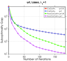
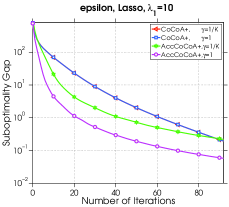
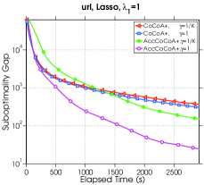
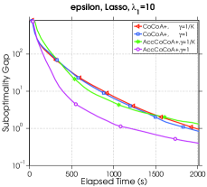
An Accelerated Communication-Efficient Primal-Dual Optimization Framework for Structured Machine Learning111This material is based upon work supported by the U.S. National Science Foundation, Division of Computing and Communications Foundations, under Award Number CCF-1618717.

Chenxin Ma222Department of Industrial and Systems Engineering, Lehigh University, Bethlehem, PA, USA; , ,    Martin Jaggi333School of Computer and Communication Sciences, École Polytechnique Fédérale de Lausanne, Lausanne, Switzerland;    Frank E. Curtis222Department of Industrial and Systems Engineering, Lehigh University, Bethlehem, PA, USA; , ,    Nathan Srebro444Toyota Technological Institute at Chicago, Chicago, IL;    Martin Takáč222Department of Industrial and Systems Engineering, Lehigh University, Bethlehem, PA, USA; , , chm514@lehigh.edu frank.e.curtis@gmail.com takac@lehigh.edu martin.jaggi@epfl.ch nati@ttic.edu
Abstract

Distributed optimization algorithms are essential for training machine learning models on very large-scale datasets. However, they often suffer from communication bottlenecks. Confronting this issue, a communication-efficient primal-dual coordinate ascent framework (CoCoA) and its improved variant CoCoA+ have been proposed, achieving a convergence rate of 𝒪(1/t)𝒪1𝑡\mathcal{O}(1/t) for solving empirical risk minimization problems with Lipschitz continuous losses. In this paper, an accelerated variant of CoCoA+ is proposed and shown to possess a convergence rate of 𝒪(1/t2)𝒪1superscript𝑡2\mathcal{O}(1/t^{2}) in terms of reducing suboptimality. The analysis of this rate is also notable in that the convergence rate bounds involve constants that, except in extreme cases, are significantly reduced compared to those previously provided for CoCoA+. The results of numerical experiments are provided to show that acceleration can lead to significant performance gains.

1 Introduction

The use of distributed optimization has become essential for training machine learning models on very large datasets. For example, distribution is a key ingredient when the dataset does not fit into the memory of a single machine, and rather must be stored in a distributed manner over many machines or computational agents, each having access only to their own (local) segment of the training data.

Efficiently training a machine learning model in such a network setting is challenging due to the cost of communicating information between machines, as compared to the relatively cheap cost of local computation on a single machine. Therefore, designing efficient distributed optimization algorithms, which are able to balance the amount of local computation with the amount of necessary communication between machines, is of crucial importance. This is especially the case since communication bottlenecks and the heterogeneity of large-scale computing systems have been increasing.

In this paper, we improve the existing CoCoA+ framework for communication-efficient distributed optimization [6, 10, 17] by equipping it with acceleration [12]. We do not simply apply a generic acceleration scheme, e.g., using the Universal Catalyst [7] (see §1.2 for more discussion), but rather develop a technique specific for our setting. We prove that our accelerated scheme possesses an improved convergence rate involving reduced constants compared to that of CoCoA+. Our theory holds for arbitrary local solvers used on the worker machines. We also provide the results of extensive numerical experiments, where we demonstrate that the new accelerated scheme leads to significantly improved performance in real application settings.

1.1 Preliminaries

We present our algorithmic framework in the context of solving the following pair of optimization problems, which are dual to each other:

(A) min𝜶nsubscript𝜶superscript𝑛\displaystyle\min_{{\boldsymbol{\alpha}}\in\mathbb{R}^{n}}\ [𝒪A(𝜶):=f(A𝜶)+igi(αi)]anddelimited-[]assignsubscript𝒪𝐴𝜶𝑓𝐴𝜶subscript𝑖subscript𝑔𝑖subscript𝛼𝑖and\displaystyle\Big{[}\ \mathcal{O}_{A}({\boldsymbol{\alpha}}):=f(A{\boldsymbol{\alpha}})\,+\,\textstyle\sum_{i\in\mathcal{I}}g_{i}(\alpha_{i})\Big{]}\quad\text{and}\,
(B) min𝐰dsubscript𝐰superscript𝑑\displaystyle\min_{{\bf w}\in\mathbb{R}^{d}}\ [𝒪B(𝐰):=f(𝐰)+igi(Ai𝐰)].delimited-[]assignsubscript𝒪𝐵𝐰superscript𝑓𝐰subscript𝑖superscriptsubscript𝑔𝑖superscriptsubscript𝐴𝑖top𝐰\displaystyle\Big{[}\ \mathcal{O}_{B}({\bf w}):=f^{*}({\bf w})\,+\,\textstyle\sum_{i\in\mathcal{I}}g_{i}^{*}(-A_{i}^{\top}{\bf w})\Big{]}.

Here, hsuperscripth^{*} denotes the convex conjugate of a function hh. The two problems are defined by the functions f:d:𝑓superscript𝑑f:\mathbb{R}^{d}\rightarrow\mathbb{R} and gi::subscript𝑔𝑖g_{i}:\mathbb{R}\rightarrow\mathbb{R} for all i𝑖i\in\mathcal{I} and a data matrix Ad×n𝐴superscript𝑑𝑛A\in\mathbb{R}^{d\times n}, about which we make the following assumption.

Assumption 1.

The functions f𝑓f and gisubscript𝑔𝑖g_{i} for all i𝑖i\in\mathcal{I} are closed and convex. In addition, the gradient function f𝑓\nabla f is Lipschitz continuous with constant λ𝜆\lambda and the function gisuperscriptsubscript𝑔𝑖g_{i}^{*} for each i𝑖i\in\mathcal{I} is Lipschitz continuous with constant L𝐿L. Finally, without loss of generality, the columns of the data matrix satisfy Ai1normsubscript𝐴𝑖1\|A_{i}\|\leq 1.

Observe that problem formulation (A) includes many important problems with nonsmooth regularizers, such as Lasso with 1subscript1\ell_{1}-norm regularization, i.e.,

(1) min𝜶nsubscript𝜶superscript𝑛\displaystyle\min_{{\boldsymbol{\alpha}}\in\mathbb{R}^{n}}\ 12A𝜶𝐛22+λ1𝜶1.12superscriptsubscriptnorm𝐴𝜶𝐛22subscript𝜆1subscriptnorm𝜶1\displaystyle\tfrac{1}{2}\left\|A{\boldsymbol{\alpha}}-{\bf b}\right\|_{2}^{2}+\lambda_{1}\|{\boldsymbol{\alpha}}\|_{1}.

More generally, many other smooth data-fitting functions can be used in place of f𝑓f in our context of problem (A). Problem formulation (B) includes many regularized empirical loss minimization problems with strongly convex regularizers of the form

(2) min𝐰dsubscript𝐰superscript𝑑\displaystyle\min_{{\bf w}\in\mathbb{R}^{d}}\ 1ni=1ni(Ai𝐰)+λ2𝐰2,1𝑛superscriptsubscript𝑖1𝑛subscript𝑖superscriptsubscript𝐴𝑖top𝐰𝜆2superscriptnorm𝐰2\displaystyle\tfrac{1}{n}\sum_{i=1}^{n}\ell_{i}(A_{i}^{\top}{\bf w})+\tfrac{\lambda}{2}\|{\bf w}\|^{2},

such as support vector machines (SVMs) or logistic regression. Here, the i𝑖i-th column Aidsubscript𝐴𝑖superscript𝑑A_{i}\in\mathbb{R}^{d} of A𝐴A represents the i𝑖i-th data example and λ>0𝜆0\lambda>0 is a regularization parameter.

1.2 Motivation and Literature Review

The increased size of optimization problems of interest in machine learning, as well as the availability of parallel and distributed architectures, has led to various directions of research on the design of parallel algorithms for either solving (1) directly (e.g., see [2, 13, 3]) or indirectly by solving its dual (2) (e.g., see [18, 8, 19]). For example, some previous work has focused on shared memory systems in which the amount of parallelism possible is dependent upon the number of processing units (CPUs) on a single node, which is usually in the range of 16–64 cores per node in a contemporary high performance cluster. To avoid locking and, hence, improve speed, some asynchronous algorithms have been proposed and analyzed [8, 13]. However, despite the fact that such methods are efficient with shared memory, naïve extensions of these ideas to distributed environments can be terribly inefficient. This is due to the fact that such naïve extensions require constant communication between nodes, causing them to suffer large overhead.

This type of observation has led many to conclude that, in a distributed computing environment, one must focus not only on the number of data accesses, but also on the number of communication steps, which is usually tied to the number of iterations of the overall optimization algorithm [9]. For this reason, researchers have proposed the use of batch (i.e., full gradient) methods, potentially using (partial or approximate) second-order information as in Newton’s method [16, 21] or a quasi-Newton method such as L-BFGS [22]. The benefit of such methods is that they typically require fewer iterations to achieve high accuracy of the solution. On the other hand, a Newton-type method requires that a linear system be solved (approximately) in every iteration. A popular approach for this procedure is the linear conjugate gradient (CG) algorithm, such as proposed in Disco [21]. Unfortunately, however, in many applications one might need a substantial number of CG steps in each Newton iteration. Since each CG step requires one pass over the data and one round of communication, this can also lead to substantial communication overhead.

To overcome these issues, the algorithms CoCoA [6], DisDCA [20] and CoCoA+ [10, 17] have been proposed to efficiently balance computation and communication in distributed optimization environments. The main idea of these methods, with the data partitioned across any number of nodes in a cluster, is to define meaningful auxiliary subproblems to be solved in each node using only locally stored data. These subproblems involve some inherited (partial) second-order information, which aids in yielding overall fast convergence for solving the original problems (A) and (B).

As is the case for many other optimization methods for machine learning, the existing CoCoA+ framework only yields a sublinear convergence rate of 𝒪(1/t)𝒪1𝑡\mathcal{O}(1/t) for the general convex case. That said, we are motivated by the fact that several single machine solvers can be improved by incorporating Nesterov acceleration [12, 1], leading to an improved rate of 𝒪(1/t2)𝒪1superscript𝑡2\mathcal{O}(1/t^{2}); e.g., this was recently successfully done in [14]. In this paper, we are able to provably accelerate the distributed CoCoA+ framework, achieving a 𝒪(1/t2)𝒪1superscript𝑡2\mathcal{O}(1/t^{2}) rate for reducing suboptimality.

It is worthwhile to mention that acceleration could be achieved using the Universal Catalyst proposed in [7]. However, for our purposes, this approach is less appealing since it does not allow the local solver to produce randomized solutions which might only have sufficient quality in expectation. Perhaps the accelerated algorithms most relevant to the present work are those in [11, 5]. The subproblems in these papers are assumed to be strongly convex. In our case, this is not general enough; instead, we manage to exploit the general structure of the objective 𝒪Asubscript𝒪𝐴\mathcal{O}_{A}.

1.3 Contributions

Overall, the contributions represented by the work in this paper can be summarized as follows. Here, for any 𝜶n𝜶superscript𝑛{\boldsymbol{\alpha}}\in\mathbb{R}^{n} in the context of (A), we define a corresponding dual solution 𝐰d𝐰superscript𝑑{\bf w}\in\mathbb{R}^{d} for problem (B) as

(3) 𝐰=𝐰(𝜶):=f(A𝜶).𝐰𝐰𝜶assign𝑓𝐴𝜶{\bf w}={\bf w}({\boldsymbol{\alpha}}):=\nabla f(A{\boldsymbol{\alpha}})\,.
  • We propose and analyze an accelerated communication-efficient block descent algorithm for solving problems (A) and (B). Our analysis shows that our framework possesses a convergence rate of 𝒪(1/t2)𝒪1superscript𝑡2\mathcal{O}(1/t^{2}) for suboptimality, i.e., with 𝜶tsubscript𝜶𝑡{\boldsymbol{\alpha}}_{t} representing the t𝑡t-th algorithm iterate, we prove the accelerated reduction of 𝒪A(𝜶t)𝒪A(𝜶)subscript𝒪𝐴subscript𝜶𝑡subscript𝒪𝐴subscript𝜶\mathcal{O}_{A}({\boldsymbol{\alpha}}_{t})-\mathcal{O}_{A}({\boldsymbol{\alpha}}_{\star}) over time t𝑡t, where 𝜶subscript𝜶{\boldsymbol{\alpha}}_{\star} represents an optimal solution of (A). Given the recent work in [4], our results for reducing suboptimality can then also be cast in terms of an accelerated rate of the duality gap G(𝜶):=𝒪A(𝜶)+𝒪B(𝐰(𝜶))assign𝐺𝜶subscript𝒪𝐴𝜶subscript𝒪𝐵𝐰𝜶G({\boldsymbol{\alpha}}):=\mathcal{O}_{A}({\boldsymbol{\alpha}})+\mathcal{O}_{B}({\bf w}({\boldsymbol{\alpha}})), as a practically important accuracy certificate.

  • The convergence analyses of CoCoA and CoCoA+ yielded bounds involving quantities which depend on the Lipschitz constants for the local subproblems. In this sense, the results might be no better than similar bounds for inexact block proximal gradient descent. By contrast, in this paper, we exploit the structure of the dual objective 𝒪Bsubscript𝒪𝐵\mathcal{O}_{B} to obtain complexity bounds that do not depend on Lipschitz constants of the auxiliary subproblems. Instead, our bounds merely depend on quantities related to local curvature corresponding to the subproblems.

  • We extend our accelerated framework to also cover general non-strongly convex regularizers. This is important, e.g., in the context of 1subscript1\ell_{1}-norm regularized Lasso, sparse logistic regression, and elastic net regularized problems.

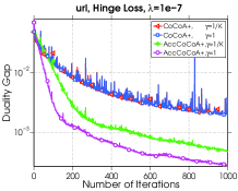
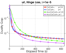
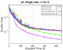
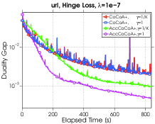
  • We have performed numerous numerical experiments to demonstrate that acceleration can lead to significant performance improvements. In particular, the gains are especially large for small values of the regularization parameter λ𝜆\lambda, which is important in very-large-scale settings where one often desires the regularization to be inversely proportional to n𝑛n. The C++ code for our implementation of our framework is available on github: https://github.com/schemmy/CoCoA-Experiments.

1.4 Organization

The remainder of the paper is organized as follows. We start by introducing our new accelerated CoCoA+ (AccCoCoA+) algorithm, including the design of its subproblems and strategies for solving them. We then describe our main complexity result for the algorithm, showing its improvement over that for CoCoA+. Finally, we comment on the results of our numerical experiments.

2 Accelerated CoCoA+

In this section, we introduce our proposed accelerated CoCoA+ (AccCoCoA+) algorithm. We begin by defining notation related to the manner in which data is distributed across various machines, then define quantities related to the local subproblems to be solved in each iteration of the algorithm. Of central importance for these subproblems are a carefully defined regularization scheme and a loose assumption on the accuracy to which each subproblem must be solved in each step of AccCoCoA+.

2.1 Data Partitioning

Suppose that the n𝑛n columns of the dataset are split across K𝐾K machines (nodes). Let the index set of columns stored on node k[K]:={1,,k}𝑘delimited-[]𝐾assign1𝑘k\in[K]:=\{1,\dots,k\} be denoted as 𝒫ksubscript𝒫𝑘\mathcal{P}_{k}. We assume that the dataset is partitioned in a disjoint manner such that 𝒫i𝒫j=subscript𝒫𝑖subscript𝒫𝑗\mathcal{P}_{i}\cap\mathcal{P}_{j}=\emptyset for any ij𝑖𝑗i\neq j while k=1K𝒫k=[n]superscriptsubscript𝑘1𝐾subscript𝒫𝑘delimited-[]𝑛\cup_{k=1}^{K}\mathcal{P}_{k}=[n]. For notational convenience, we split the variable vector 𝜶n𝜶superscript𝑛{\boldsymbol{\alpha}}\in\mathbb{R}^{n} into the set of K𝐾K vectors {𝜶[k]}k=1Ksuperscriptsubscriptsuperscript𝜶delimited-[]𝑘𝑘1𝐾\{{\boldsymbol{\alpha}}^{[k]}\}_{k=1}^{K} by employing, for each k[K]𝑘delimited-[]𝐾k\in[K], the masking operator

(4) (𝜶[k])i:={αiifi𝒫k,0otherwise.assignsubscriptsuperscript𝜶delimited-[]𝑘𝑖casessubscript𝛼𝑖if𝑖subscript𝒫𝑘0otherwise.{({\boldsymbol{\alpha}}^{[k]})}_{i}:=\begin{cases}\alpha_{i}&\mbox{if}\ i\in\mathcal{P}_{k},\\ 0&\mbox{otherwise.}\end{cases}

As a consequence of separability of g𝑔g in (A), we write

(5) ψk(𝜶[k]):=i𝒫kgi(αi),assignsubscript𝜓𝑘superscript𝜶delimited-[]𝑘subscript𝑖subscript𝒫𝑘subscript𝑔𝑖subscript𝛼𝑖\psi_{k}({\boldsymbol{\alpha}}^{[k]}):=\sum_{i\in\mathcal{P}_{k}}g_{i}(\alpha_{i}),

so that g(𝜶)=k=1Kψk(𝜶[k])𝑔𝜶superscriptsubscript𝑘1𝐾subscript𝜓𝑘superscript𝜶delimited-[]𝑘g({\boldsymbol{\alpha}})=\sum_{k=1}^{K}\psi_{k}({\boldsymbol{\alpha}}^{[k]}).

2.2 Subproblem

Iteration t𝑡t of AccCoCoA+ involves the auxiliary vectors (𝐲t,𝐳t)n×nsubscript𝐲𝑡subscript𝐳𝑡superscript𝑛superscript𝑛({\bf y}_{t},{\bf z}_{t})\in\mathbb{R}^{n}\times\mathbb{R}^{n}, which one may split into {𝐲t[k]}k=1Ksuperscriptsubscriptsuperscriptsubscript𝐲𝑡delimited-[]𝑘𝑘1𝐾\{{\bf y}_{t}^{[k]}\}_{k=1}^{K} and {𝐳t[k]}k=1Ksuperscriptsubscriptsuperscriptsubscript𝐳𝑡delimited-[]𝑘𝑘1𝐾\{{\bf z}_{t}^{[k]}\}_{k=1}^{K}, respectively, in the same manner as 𝜶n𝜶superscript𝑛{\boldsymbol{\alpha}}\in\mathbb{R}^{n} in (4). Fundamentally, the goal in iteration t𝑡t on each node k[K]𝑘delimited-[]𝐾k\in[K] is to (approximately) solve

(6) min𝐳t+1[k]n𝒢k(𝐳t+1[k];𝐲t,𝐳t),subscriptsuperscriptsubscript𝐳𝑡1delimited-[]𝑘superscript𝑛subscript𝒢𝑘superscriptsubscript𝐳𝑡1delimited-[]𝑘subscript𝐲𝑡subscript𝐳𝑡\displaystyle\min_{{\bf z}_{t+1}^{[k]}\in\mathbb{R}^{n}}\mathcal{G}_{k}({\bf z}_{t+1}^{[k]};{\bf y}_{t},{\bf z}_{t}),

where, for scalars σ0superscript𝜎0\sigma^{\prime}\geq 0 and θt0subscript𝜃𝑡0\theta_{t}\geq 0 (see below), the local objective function is

𝒢k(𝐳t+1[k];𝐲t,𝐳t):=assignsubscript𝒢𝑘superscriptsubscript𝐳𝑡1delimited-[]𝑘subscript𝐲𝑡subscript𝐳𝑡absent\displaystyle\mathcal{G}_{k}({\bf z}_{t+1}^{[k]};{\bf y}_{t},{\bf z}_{t}):= ψk(𝐳t+1[k])+1Kf(A𝐲t)subscript𝜓𝑘superscriptsubscript𝐳𝑡1delimited-[]𝑘1𝐾𝑓𝐴subscript𝐲𝑡\displaystyle\ \psi_{k}({\bf z}_{t+1}^{[k]})+\frac{1}{K}f(A{\bf y}_{t})
(7) +f(A𝐲t)A(𝐳t+1[k]𝐲t[k])+λθtσ2A(𝐳t+1[k]𝐳t[k])2.𝑓superscript𝐴subscript𝐲𝑡top𝐴superscriptsubscript𝐳𝑡1delimited-[]𝑘subscriptsuperscript𝐲delimited-[]𝑘𝑡𝜆subscript𝜃𝑡superscript𝜎2superscriptnorm𝐴superscriptsubscript𝐳𝑡1delimited-[]𝑘subscriptsuperscript𝐳delimited-[]𝑘𝑡2\displaystyle+\nabla f(A{\bf y}_{t})^{\top}A({\bf z}_{t+1}^{[k]}-{\bf y}^{[k]}_{t})+\frac{\lambda\theta_{t}\sigma^{\prime}}{2}\left\|A({\bf z}_{t+1}^{[k]}-{\bf z}^{[k]}_{t})\right\|^{2}.

At first glance, it is not obvious that this subproblem can be solved only using local data on node k𝑘k due to the presence of the term f(A𝐲t)A(𝐳t+1[k]𝐲t[k])𝑓superscript𝐴subscript𝐲𝑡top𝐴superscriptsubscript𝐳𝑡1delimited-[]𝑘subscriptsuperscript𝐲delimited-[]𝑘𝑡\nabla f(A{\bf y}_{t})^{\top}A({\bf z}_{t+1}^{[k]}-{\bf y}^{[k]}_{t}), which is dependent on the entire dataset. However, by simply making the single shared vector 𝐰t:=f(A𝐲t)assignsubscript𝐰𝑡𝑓𝐴subscript𝐲𝑡{\bf w}_{t}:=\nabla f(A{\bf y}_{t}) available on each node, the local subproblem (6) only requires knowledge of the pair (𝐲t[k],𝐳t[k])superscriptsubscript𝐲𝑡delimited-[]𝑘superscriptsubscript𝐳𝑡delimited-[]𝑘({\bf y}_{t}^{[k]},{\bf z}_{t}^{[k]}) and the local part of A𝐴A, and not the full vectors (𝐲t,𝐳t)subscript𝐲𝑡subscript𝐳𝑡({\bf y}_{t},{\bf z}_{t}). Therefore, the storage of the variable vectors 𝐲𝐲{\bf y} and 𝐳𝐳{\bf z} can also be distributed.

The last term in (2.2) represents a regularization term in which the parameter σ0superscript𝜎0\sigma^{\prime}\geq 0 plays a critical role. In short, it can be interpreted as a measure for the cross-dependency of the partitioning of the data. For our analysis, this term must be chosen, for some γ[1K,1]𝛾1𝐾1\gamma\in[\tfrac{1}{K},1], to satisfy

(8) σσmin:=γmax𝜶RnA𝜶2k=1KA𝜶[k]2.superscript𝜎subscriptsuperscript𝜎𝑚𝑖𝑛assign𝛾subscript𝜶superscript𝑅𝑛superscriptnorm𝐴𝜶2superscriptsubscript𝑘1𝐾superscriptnorm𝐴superscript𝜶delimited-[]𝑘2\sigma^{\prime}\geq\sigma^{\prime}_{min}:=\gamma\max_{{\boldsymbol{\alpha}}\in\\ R^{n}}\frac{\|A{\boldsymbol{\alpha}}\|^{2}}{\sum_{k=1}^{K}\|A{\boldsymbol{\alpha}}^{[k]}\|^{2}}.

It is easy to show that σmin/γ=max𝜶RnA𝜶2k=1KA𝜶[k]2[1,K]subscriptsuperscript𝜎𝑚𝑖𝑛𝛾subscript𝜶superscript𝑅𝑛superscriptnorm𝐴𝜶2superscriptsubscript𝑘1𝐾superscriptnorm𝐴superscript𝜶delimited-[]𝑘21𝐾\sigma^{\prime}_{min}/\gamma=\max_{{\boldsymbol{\alpha}}\in\\ R^{n}}\frac{\|A{\boldsymbol{\alpha}}\|^{2}}{\sum_{k=1}^{K}\|A{\boldsymbol{\alpha}}^{[k]}\|^{2}}\in[1,K]. If it is equal to 1, then any pair of samples from different elements of the partition must be orthogonal to each other. In such cases, the function 𝒪Asubscript𝒪𝐴\mathcal{O}_{A} is block-separable. On the other hand, if σmin/γsubscriptsuperscript𝜎𝑚𝑖𝑛𝛾\sigma^{\prime}_{min}/\gamma is close to K𝐾K, then the data across the partition are strongly correlated. Note that the choice σ=γKsuperscript𝜎𝛾𝐾\sigma^{\prime}=\gamma K is “safe” in the sense that (8) holds; see [10, Lemma 4].

2.3 Approximate Subproblem Solutions

A strength of our framework is that each subproblem (6) need not be solved exactly. This is critical since, in the extreme, solving the subproblems exactly can be as difficult as solving the original problem. In AccCoCoA+, we make the assumption that, in iteration t𝑡t, the solver employed to solve the subproblem on node k𝑘k yields an approximate solution with some additive error ϵt0subscriptitalic-ϵ𝑡0\epsilon_{t}\geq 0. To be precise, we make the following assumption.

Assumption 2 (ϵtsubscriptitalic-ϵ𝑡\epsilon_{t}-approximate solutions).

There exists a sequence {ϵt}t=00superscriptsubscriptsubscriptitalic-ϵ𝑡𝑡00\{\epsilon_{t}\}_{t=0}^{\infty}\geq 0 such that, for each t{0,1,2,}𝑡012t\in\{0,1,2,\dots\} and k[K]𝑘delimited-[]𝐾k\in[K], the local solver employed on node k𝑘k in iteration t𝑡t produces a (possibly random) 𝐳t+1[k]superscriptsubscript𝐳𝑡1delimited-[]𝑘{\bf z}_{t+1}^{[k]} satisfying

(9) 𝐄t+1[𝒢k(𝐳t+1[k];𝐲t,𝐳t)|t]𝒢k(𝐳t+1[k];𝐲t,𝐳t)+ϵt,subscript𝐄𝑡1conditionalsubscript𝒢𝑘superscriptsubscript𝐳𝑡1delimited-[]𝑘subscript𝐲𝑡subscript𝐳𝑡𝑡subscript𝒢𝑘superscriptsuperscriptsubscript𝐳𝑡1delimited-[]𝑘subscript𝐲𝑡subscript𝐳𝑡subscriptitalic-ϵ𝑡\operatorname{\mathbf{E}}_{t+1}[\mathcal{G}_{k}({\bf z}_{t+1}^{[k]};{\bf y}_{t},{\bf z}_{t})|t]\leq\mathcal{G}_{k}({{\bf z}_{t+1}^{\star}}^{[k]};{\bf y}_{t},{\bf z}_{t})+\epsilon_{t},

where 𝐳t+1[k]:=argmin𝐳t+1[k]n𝒢k(𝐳t+1[k];𝐲t,𝐳t)assignsuperscriptsuperscriptsubscript𝐳𝑡1delimited-[]𝑘subscriptsuperscriptsubscript𝐳𝑡1delimited-[]𝑘superscript𝑛subscript𝒢𝑘superscriptsubscript𝐳𝑡1delimited-[]𝑘subscript𝐲𝑡subscript𝐳𝑡{{\bf z}_{t+1}^{\star}}^{[k]}:=\arg\min_{{\bf z}_{t+1}^{[k]}\in\mathbb{R}^{n}}\mathcal{G}_{k}({\bf z}_{t+1}^{[k]};{\bf y}_{t},{\bf z}_{t}) and 𝐄t+1[|t]\operatorname{\mathbf{E}}_{t+1}[\cdot|t] indicates conditional expectation given the algorithm history up to time t𝑡t.

2.4 Algorithm

AccCoCoA+ is stated as Algorithm 1. Given an initial iterate vector 𝜶0subscript𝜶0{\boldsymbol{\alpha}}_{0} in the effective domain of g𝑔g and the scalar θ0=1subscript𝜃01\theta_{0}=1, each iteration involves a series of steps, only one of which involves communication between nodes. First, the auxiliary vectors {𝐲t[k]}k=1Ksuperscriptsubscriptsuperscriptsubscript𝐲𝑡delimited-[]𝑘𝑘1𝐾\{{\bf y}_{t}^{[k]}\}_{k=1}^{K} are set on each node, each representing a convex combination of the variables 𝜶t[k]superscriptsubscript𝜶𝑡delimited-[]𝑘{\boldsymbol{\alpha}}_{t}^{[k]} and 𝐳t[k]superscriptsubscript𝐳𝑡delimited-[]𝑘{\bf z}_{t}^{[k]}. Then, for setting up the local objective (2.2) for each subproblem (6), the combined vector 𝐲tsubscript𝐲𝑡{\bf y}_{t} is used to compute 𝐰tsubscript𝐰𝑡{\bf w}_{t}, which must be communicated to all nodes. After this point in iteration t𝑡t, all remaining steps involve local computation on each node: each subproblem is solved approximately to compute {𝐳t+1[k]}k=1Ksuperscriptsubscriptsuperscriptsubscript𝐳𝑡1delimited-[]𝑘𝑘1𝐾\{{\bf z}_{t+1}^{[k]}\}_{k=1}^{K}, after which the elements of {𝜶t+1[k]}k=1Ksuperscriptsubscriptsuperscriptsubscript𝜶𝑡1delimited-[]𝑘𝑘1𝐾\{{\boldsymbol{\alpha}}_{t+1}^{[k]}\}_{k=1}^{K} are set. Acceleration of the algorithm is due to the careful update for the sequence {θt}subscript𝜃𝑡\{\theta_{t}\}, which, since it only involves a prescribed formula for a scalar quantity, can be performed identically on each node. Observe that the update sequence ensures that θt𝒪(1/t)similar-tosubscript𝜃𝑡𝒪1𝑡\theta_{t}\sim\mathcal{O}(1/t).

Algorithm 1 Accelerated CoCoA+ (AccCoCoA+)
1:  choose 𝜶0dom(g)𝐑nsubscript𝜶0dom𝑔superscript𝐑𝑛{\boldsymbol{\alpha}}_{0}\in\operatorname{dom}(g)\subseteq\mathbf{R}^{n}; set 𝐳0:=𝜶0assignsubscript𝐳0subscript𝜶0{\bf z}_{0}:={\boldsymbol{\alpha}}_{0}, γ[1K,1]𝛾1𝐾1\gamma\in[\tfrac{1}{K},1] and θ0:=1assignsubscript𝜃01\theta_{0}:=1
2:  for t{0,1,2,}𝑡012t\in\{0,1,2,\dots\} do
3:     for k[K]𝑘delimited-[]𝐾k\in[K] in parallel, set
(10) 𝐲t[k]:=(1γθt)𝜶t[k]+γθt𝐳t[k]assignsubscriptsuperscript𝐲delimited-[]𝑘𝑡1𝛾subscript𝜃𝑡subscriptsuperscript𝜶delimited-[]𝑘𝑡𝛾subscript𝜃𝑡subscriptsuperscript𝐳delimited-[]𝑘𝑡{\bf y}^{[k]}_{t}:=(1-\gamma\theta_{t}){\boldsymbol{\alpha}}^{[k]}_{t}+\gamma\theta_{t}{\bf z}^{[k]}_{t}\vspace{-3mm}
4:     set 𝐰t:=f(A𝐲t)assignsubscript𝐰𝑡𝑓𝐴subscript𝐲𝑡{\bf w}_{t}:=\nabla f(A{\bf y}_{t}) and communicate to all nodes
5:     for k[K]𝑘delimited-[]𝐾k\in[K] in parallel, compute an ϵtsubscriptitalic-ϵ𝑡\epsilon_{t}-approximate solution 𝐳t+1[k]superscriptsubscript𝐳𝑡1delimited-[]𝑘{\bf z}_{t+1}^{[k]} of subproblem (6)
6:     for k[K]𝑘delimited-[]𝐾k\in[K] in parallel, set
(11) 𝜶t+1[k]:=𝐲t[k]+γθt(𝐳t+1[k]𝐳t[k])assignsubscriptsuperscript𝜶delimited-[]𝑘𝑡1subscriptsuperscript𝐲delimited-[]𝑘𝑡𝛾subscript𝜃𝑡subscriptsuperscript𝐳delimited-[]𝑘𝑡1subscriptsuperscript𝐳delimited-[]𝑘𝑡{\boldsymbol{\alpha}}^{[k]}_{t+1}:={\bf y}^{[k]}_{t}+\gamma\theta_{t}({\bf z}^{[k]}_{t+1}-{\bf z}^{[k]}_{t})\vspace{-3mm}
7:     set θt+1:=γ2θt4+4θt2γθt22assignsubscript𝜃𝑡1superscript𝛾2superscriptsubscript𝜃𝑡44superscriptsubscript𝜃𝑡2𝛾superscriptsubscript𝜃𝑡22\theta_{t+1}:=\frac{\sqrt{\gamma^{2}\theta_{t}^{4}+4\theta_{t}^{2}}-\gamma\theta_{t}^{2}}{2} (on each node)
8:  end for

3 Convergence Analysis

In this section, we study the convergence properties of the proposed AccCoCoA+ algorithm. First, we prove general complexity results, then, respectively in Sections 3.1 and 3.2, we provide interpretations of this main theorem for cases when the subproblems are solved exactly or inexactly.

First, we prove the following lemma related to the sequence {θt}t0subscriptsubscript𝜃𝑡𝑡0\{\theta_{t}\}_{t\geq 0}. The result is similar to that given as Lemma 1 in [5].

Lemma 3.1.

The sequence {θt}t0subscriptsubscript𝜃𝑡𝑡0\{\theta_{t}\}_{t\geq 0} is positive, monotonically decreasing, and has

(12) 1γθt+1θt+12=1θt21𝛾subscript𝜃𝑡1subscriptsuperscript𝜃2𝑡11subscriptsuperscript𝜃2𝑡\frac{1-\gamma\theta_{t+1}}{\theta^{2}_{t+1}}=\frac{1}{\theta^{2}_{t}}

and

(13) θt2tγ+21subscript𝜃𝑡2𝑡𝛾21\theta_{t}\leq\frac{2}{t\gamma+2}\leq 1

for all t0𝑡0t\geq 0.

Proof 3.2.

For each t0𝑡0t\geq 0, the value θt+1subscript𝜃𝑡1\theta_{t+1} can be seen from Step 7 of Algorithm 1 to be the positive root of the quadratic equation

(14) θ2+(γθt2)θθt2=0.superscript𝜃2𝛾superscriptsubscript𝜃𝑡2𝜃superscriptsubscript𝜃𝑡20\theta^{2}+(\gamma\theta_{t}^{2})\theta-\theta_{t}^{2}=0.

Since θ0=1subscript𝜃01\theta_{0}=1, it follows from (14), the fact that a strongly convex quadratic univariate function with a negative vertical intercept has a positive real root, and a simple inductive argument that θt>0subscript𝜃𝑡0\theta_{t}>0 for all t0𝑡0t\geq 0, as desired. Next, plugging in θt+1subscript𝜃𝑡1\theta_{t+1} for θ𝜃\theta in (14) and rearranging, we obtain (12). This can again be rearranged to yield

(15) 1θt+12=1θt2+γθt+1,1superscriptsubscript𝜃𝑡121superscriptsubscript𝜃𝑡2𝛾subscript𝜃𝑡1\frac{1}{\theta_{t+1}^{2}}=\frac{1}{\theta_{t}^{2}}+\frac{\gamma}{\theta_{t+1}},

from which it follows that

1θt2=1+i=1tγθifor all t0.1superscriptsubscript𝜃𝑡21superscriptsubscript𝑖1𝑡𝛾subscript𝜃𝑖for all t0\frac{1}{\theta_{t}^{2}}=1+\sum_{i=1}^{t}\frac{\gamma}{\theta_{i}}\ \ \text{for all $t\geq 0$}.

This shows that {θt}t0subscriptsubscript𝜃𝑡𝑡0\{\theta_{t}\}_{t\geq 0} is monotonically decreasing, as desired. We now use mathematical induction to show (13). First, (13) clearly holds for t=0𝑡0t=0, for which we have θ0=20+2=1subscript𝜃02021\theta_{0}=\frac{2}{0+2}=1. Assuming it holds up to t𝑡t, we have from (15) that

(16) 1θt+12γθt+1=1θt2(γt+2)24.1superscriptsubscript𝜃𝑡12𝛾subscript𝜃𝑡11superscriptsubscript𝜃𝑡2superscript𝛾𝑡224\frac{1}{\theta_{t+1}^{2}}-\frac{\gamma}{\theta_{t+1}}=\frac{1}{\theta_{t}^{2}}\geq\frac{(\gamma t+2)^{2}}{4}.

Now observe that the quadratic equation in the variable 1/θ1𝜃1/\theta given by

1θ2γθ(γt+2)24=0has roots1θ=γ±γ2+(γt+2)22.formulae-sequence1superscript𝜃2𝛾𝜃superscript𝛾𝑡2240has roots1𝜃plus-or-minus𝛾superscript𝛾2superscript𝛾𝑡222\displaystyle\frac{1}{\theta^{2}}-\frac{\gamma}{\theta}-\frac{(\gamma t+2)^{2}}{4}=0\ \ \text{has roots}\ \ \frac{1}{\theta}=\frac{\gamma\pm\sqrt{\gamma^{2}+(\gamma t+2)^{2}}}{2}.

This shows that, by (16) and since θt+1>0subscript𝜃𝑡10\theta_{t+1}>0, we have

1θt+1γ+γ2+(γt+2)22γ+(γt+2)22=γ(t+1)+22.1subscript𝜃𝑡1𝛾superscript𝛾2superscript𝛾𝑡222𝛾superscript𝛾𝑡222𝛾𝑡122\displaystyle\frac{1}{\theta_{t+1}}\geq\frac{\gamma+\sqrt{\gamma^{2}+(\gamma t+2)^{2}}}{2}\geq\frac{\gamma+\sqrt{(\gamma t+2)^{2}}}{2}=\frac{\gamma(t+1)+2}{2}.

Therefore, we conclude θt+12(t+1)γ+21subscript𝜃𝑡12𝑡1𝛾21\theta_{t+1}\leq\frac{2}{(t+1)\gamma+2}\leq 1, which concludes the proof.

Next, we prove the following lemma, which is a modification of Lemma 2 in [5].

Lemma 3.3.

Let {𝛂t,𝐳t}t0subscriptsubscript𝛂𝑡subscript𝐳𝑡𝑡0\{{\boldsymbol{\alpha}}_{t},{\bf z}_{t}\}_{t\geq 0} be generated by Algorithm 1. Then, for all t0𝑡0t\geq 0,

(17) 𝜶t=l=0tρtl𝐳l,subscript𝜶𝑡superscriptsubscript𝑙0𝑡subscriptsuperscript𝜌𝑙𝑡subscript𝐳𝑙{\boldsymbol{\alpha}}_{t}=\sum_{l=0}^{t}{\rho^{l}_{t}{\bf z}_{l}},

where the coefficients {ρt0,ρt1,,ρtt}subscriptsuperscript𝜌0𝑡subscriptsuperscript𝜌1𝑡subscriptsuperscript𝜌𝑡𝑡\{\rho^{0}_{t},\rho^{1}_{t},...,\rho^{t}_{t}\} are nonnegative and sum to 1; i.e., 𝛂tsubscript𝛂𝑡{\boldsymbol{\alpha}}_{t} is a convex combination of the vectors {𝐳0,𝐳1,,𝐳t}subscript𝐳0subscript𝐳1subscript𝐳𝑡\{{\bf z}_{0},{\bf z}_{1},...,{\bf z}_{t}\}. More precisely, the coefficients are defined recursively in t𝑡t as ρ00=1,ρ10=1γθ0,ρ11=γθ0formulae-sequencesuperscriptsubscript𝜌001formulae-sequencesuperscriptsubscript𝜌101𝛾subscript𝜃0superscriptsubscript𝜌11𝛾subscript𝜃0\rho_{0}^{0}=1,\rho_{1}^{0}=1-\gamma\theta_{0},\rho_{1}^{1}=\gamma\theta_{0} and, for all t1𝑡1t\geq 1,

(18) ρt+1l={(1γθt)ρtlforl{0,,t},γθtforl=t+1.subscriptsuperscript𝜌𝑙𝑡1cases1𝛾subscript𝜃𝑡superscriptsubscript𝜌𝑡𝑙for𝑙0𝑡𝛾subscript𝜃𝑡for𝑙𝑡1\displaystyle\rho^{l}_{t+1}=\begin{cases}(1-\gamma\theta_{t})\rho_{t}^{l}&\text{for}\ \ l\in\{0,...,t\},\\ \gamma\theta_{t}&\text{for}\ \ l=t+1.\end{cases}

Proof 3.4.

We proceed by induction. First, notice that 𝛂0=𝐳0=ρ00𝐳0subscript𝛂0subscript𝐳0superscriptsubscript𝜌00subscript𝐳0{\boldsymbol{\alpha}}_{0}={\bf z}_{0}=\rho_{0}^{0}{\bf z}_{0} where ρ00:=1assignsuperscriptsubscript𝜌001\rho_{0}^{0}:=1. By (10), this implies that 𝐲0=𝐳0subscript𝐲0subscript𝐳0{\bf y}_{0}={\bf z}_{0}, which together with θ0=1subscript𝜃01\theta_{0}=1 gives (see (11))

𝜶1=𝐲0+γθ0(𝐳1𝐳0)=𝐳0+γθ0(𝐳1𝐳0)=(1γθ0)𝐳0+γθ0𝐳1,subscript𝜶1subscript𝐲0𝛾subscript𝜃0subscript𝐳1subscript𝐳0subscript𝐳0𝛾subscript𝜃0subscript𝐳1subscript𝐳01𝛾subscript𝜃0subscript𝐳0𝛾subscript𝜃0subscript𝐳1{\boldsymbol{\alpha}}_{1}={\bf y}_{0}+\gamma\theta_{0}({\bf z}_{1}-{\bf z}_{0})={\bf z}_{0}+\gamma\theta_{0}({\bf z}_{1}-{\bf z}_{0})=(1-\gamma\theta_{0}){\bf z}_{0}+\gamma\theta_{0}{\bf z}_{1},

which proves (17) for t=1𝑡1t=1. Assuming now that (17)italic-(17italic-)\eqref{eq:35} holds for some t1𝑡1t\geq 1, we obtain

𝜶t+1subscript𝜶𝑡1\displaystyle{\boldsymbol{\alpha}}_{t+1} =(11)𝐲t+γθt(𝐳t+1𝐳t)italic-(11italic-)subscript𝐲𝑡𝛾subscript𝜃𝑡subscript𝐳𝑡1subscript𝐳𝑡\displaystyle\overset{\eqref{afasfasfdsafa}}{=}{\bf y}_{t}+\gamma\theta_{t}({\bf z}_{t+1}-{\bf z}_{t})
=(10)(1γθt)𝜶t+γθt𝐳t+γθt(𝐳t+1𝐳t)italic-(10italic-)1𝛾subscript𝜃𝑡subscript𝜶𝑡𝛾subscript𝜃𝑡subscript𝐳𝑡𝛾subscript𝜃𝑡subscript𝐳𝑡1subscript𝐳𝑡\displaystyle\overset{\eqref{afwgrvwfeagwefrw}}{=}(1-\gamma\theta_{t}){\boldsymbol{\alpha}}_{t}+\gamma\theta_{t}{\bf z}_{t}+\gamma\theta_{t}({\bf z}_{t+1}-{\bf z}_{t})
=(17)(1γθt)l=0tρtl𝐳l+γθt𝐳t+γθt(𝐳t+1𝐳t)italic-(17italic-)1𝛾subscript𝜃𝑡superscriptsubscript𝑙0𝑡subscriptsuperscript𝜌𝑙𝑡subscript𝐳𝑙𝛾subscript𝜃𝑡subscript𝐳𝑡𝛾subscript𝜃𝑡subscript𝐳𝑡1subscript𝐳𝑡\displaystyle\overset{\eqref{eq:35}}{=}(1-\gamma\theta_{t})\sum_{l=0}^{t}{\rho^{l}_{t}{\bf z}_{l}}+\gamma\theta_{t}{\bf z}_{t}+\gamma\theta_{t}({\bf z}_{t+1}-{\bf z}_{t})
(19) =(17)l=0t(1γθt)ρtlρt+1l𝐳l+γθtρt+1t+1𝐳t+1.italic-(17italic-)superscriptsubscript𝑙0𝑡subscript1𝛾subscript𝜃𝑡subscriptsuperscript𝜌𝑙𝑡superscriptsubscript𝜌𝑡1𝑙subscript𝐳𝑙subscript𝛾subscript𝜃𝑡subscriptsuperscript𝜌𝑡1𝑡1subscript𝐳𝑡1\displaystyle\overset{\eqref{eq:35}}{=}\sum_{l=0}^{t}\underbrace{(1-\gamma\theta_{t})\rho^{l}_{t}}_{\rho_{t+1}^{l}}{\bf z}_{l}+\underbrace{\gamma\theta_{t}}_{\rho^{t+1}_{t+1}}{\bf z}_{t+1}.

From (13) and since γ[1K,1]𝛾1𝐾1\gamma\in[\frac{1}{K},1], it follows that ρt+1l0subscriptsuperscript𝜌𝑙𝑡10\rho^{l}_{t+1}\geq 0 for all l{0,,t+1}𝑙0𝑡1l\in\{0,\dots,t+1\}. It remains to show that the constants sum to 1. This is true since, for all t1𝑡1t\geq 1, the weights in (19) (for 𝛂t+1subscript𝛂𝑡1{\boldsymbol{\alpha}}_{t+1}) are obtained by taking the corresponding weights for 𝛂tsubscript𝛂𝑡{\boldsymbol{\alpha}}_{t}, multiplying them by γθt(0,1]𝛾subscript𝜃𝑡01\gamma\theta_{t}\in(0,1], then including the weight for 𝐳t+1subscript𝐳𝑡1{\bf z}_{t+1} as γθt𝛾subscript𝜃𝑡\gamma\theta_{t}.

Our next result relates to the optimal solution of an instance of subproblem (6).

Lemma 3.5.

Let 𝐮[k]:=argmin𝐮[k]𝒢k(𝐮[k];𝐲,𝐳)assignsuperscriptsuperscript𝐮delimited-[]𝑘subscriptsuperscript𝐮delimited-[]𝑘subscript𝒢𝑘superscript𝐮delimited-[]𝑘𝐲𝐳{{\bf u}^{\star}}^{[k]}:=\arg\min_{{\bf u}^{[k]}}\mathcal{G}_{k}({{\bf u}}^{[k]};{\bf y},{\bf z}). Then, for all 𝐮[k]superscript𝐮delimited-[]𝑘{\bf u}^{[k]},

(20) 𝒢k(𝐮[k];𝐲,𝐳)𝒢k(𝐮[k];𝐲,𝐳)+λθtσ2A(𝐮[k]𝐮[k])2.subscript𝒢𝑘superscript𝐮delimited-[]𝑘𝐲𝐳subscript𝒢𝑘superscriptsuperscript𝐮delimited-[]𝑘𝐲𝐳𝜆subscript𝜃𝑡superscript𝜎2superscriptnorm𝐴superscript𝐮delimited-[]𝑘superscriptsuperscript𝐮delimited-[]𝑘2\mathcal{G}_{k}({{\bf u}}^{[k]};{\bf y},{\bf z})\geq\mathcal{G}_{k}({{\bf u}^{\star}}^{[k]};{\bf y},{\bf z})+\frac{\lambda\theta_{t}\sigma^{\prime}}{2}\|A({{\bf u}}^{[k]}-{{\bf u}^{\star}}^{[k]})\|^{2}.

Proof 3.6.

Using convexity of f𝑓f and gisubscript𝑔𝑖g_{i} for all i𝑖i\in\mathcal{I} (and, therefore, convexity of ψksubscript𝜓𝑘\psi_{k} defined in (5)), one finds that for 𝐯[k]ψk(𝐮[k])superscript𝐯delimited-[]𝑘subscript𝜓𝑘superscriptsuperscript𝐮delimited-[]𝑘{\bf v}^{[k]}\in\partial\psi_{k}({{{\bf u}^{\star}}}^{[k]}) one has

𝒢k(𝐮[k];𝐲,𝐳)subscript𝒢𝑘superscript𝐮delimited-[]𝑘𝐲𝐳\displaystyle\ \mathcal{G}_{k}({{\bf u}}^{[k]};{\bf y},{\bf z})
=(2.2)italic-(2.2italic-)\displaystyle\overset{\eqref{eq:subpdef4}}{=} ψk(𝐮[k])+1Kf(A𝐲)+f(A𝐲)A(𝐮[k]𝐲[k])+λθtσ2A(𝐮[k]𝐳[k])2subscript𝜓𝑘superscript𝐮delimited-[]𝑘1𝐾𝑓𝐴𝐲𝑓superscript𝐴𝐲top𝐴superscript𝐮delimited-[]𝑘superscript𝐲delimited-[]𝑘𝜆subscript𝜃𝑡superscript𝜎2superscriptnorm𝐴superscript𝐮delimited-[]𝑘superscript𝐳delimited-[]𝑘2\displaystyle\ \psi_{k}({{\bf u}}^{[k]})+\frac{1}{K}f(A{\bf y})+\nabla f(A{\bf y})^{\top}A({{\bf u}}^{[k]}-{\bf y}^{[k]})+\frac{\lambda\theta_{t}\sigma^{\prime}}{2}\left\|A({\bf u}^{[k]}-{\bf z}^{[k]})\right\|^{2}
\displaystyle\geq ψk(𝐮[k])+𝐯[k],𝐮[k]𝐮[k]subscript𝜓𝑘superscriptsuperscript𝐮delimited-[]𝑘superscript𝐯delimited-[]𝑘superscript𝐮delimited-[]𝑘superscriptsuperscript𝐮delimited-[]𝑘\displaystyle\ \psi_{k}({{{\bf u}^{\star}}}^{[k]})+\langle{\bf v}^{[k]},{\bf u}^{[k]}-{{{\bf u}^{\star}}}^{[k]}\rangle
+1Kf(A𝐲)+f(A𝐲)A(𝐮[k]𝐮[k]+𝐮[k]𝐲[k])1𝐾𝑓𝐴𝐲𝑓superscript𝐴𝐲top𝐴superscript𝐮delimited-[]𝑘superscriptsuperscript𝐮delimited-[]𝑘superscriptsuperscript𝐮delimited-[]𝑘superscript𝐲delimited-[]𝑘\displaystyle\qquad+\frac{1}{K}f(A{\bf y})+\nabla f(A{\bf y})^{\top}A({{\bf u}}^{[k]}-{{{\bf u}^{\star}}}^{[k]}+{{{\bf u}^{\star}}}^{[k]}-{\bf y}^{[k]})
+λθtσ2A(𝐮[k]𝐮[k]+𝐮[k]𝐳[k])2𝜆subscript𝜃𝑡superscript𝜎2superscriptnorm𝐴superscript𝐮delimited-[]𝑘superscriptsuperscript𝐮delimited-[]𝑘superscriptsuperscript𝐮delimited-[]𝑘superscript𝐳delimited-[]𝑘2\displaystyle\qquad+\frac{\lambda\theta_{t}\sigma^{\prime}}{2}\left\|A({\bf u}^{[k]}-{{{\bf u}^{\star}}}^{[k]}+{{{\bf u}^{\star}}}^{[k]}-{\bf z}^{[k]})\right\|^{2}
=\displaystyle= ψk(𝐮[k])+𝐯[k],𝐮[k]𝐮[k]subscript𝜓𝑘superscriptsuperscript𝐮delimited-[]𝑘superscript𝐯delimited-[]𝑘superscript𝐮delimited-[]𝑘superscriptsuperscript𝐮delimited-[]𝑘\displaystyle\ \psi_{k}({{{\bf u}^{\star}}}^{[k]})+\langle{\bf v}^{[k]},{\bf u}^{[k]}-{{{\bf u}^{\star}}}^{[k]}\rangle
+1Kf(A𝐲)+f(A𝐲)A(𝐮[k]𝐮[k])+f(A𝐲)A(𝐮[k]𝐲[k])1𝐾𝑓𝐴𝐲𝑓superscript𝐴𝐲top𝐴superscript𝐮delimited-[]𝑘superscriptsuperscript𝐮delimited-[]𝑘𝑓superscript𝐴𝐲top𝐴superscriptsuperscript𝐮delimited-[]𝑘superscript𝐲delimited-[]𝑘\displaystyle\qquad+\frac{1}{K}f(A{\bf y})+\nabla f(A{\bf y})^{\top}A({{\bf u}}^{[k]}-{{{\bf u}^{\star}}}^{[k]})+\nabla f(A{\bf y})^{\top}A({{{\bf u}^{\star}}}^{[k]}-{\bf y}^{[k]})
+λθtσ2A(𝐮[k]𝐮[k])2+λθtσ2A(𝐮[k]𝐳[k])2𝜆subscript𝜃𝑡superscript𝜎2superscriptnorm𝐴superscript𝐮delimited-[]𝑘superscriptsuperscript𝐮delimited-[]𝑘2𝜆subscript𝜃𝑡superscript𝜎2superscriptnorm𝐴superscriptsuperscript𝐮delimited-[]𝑘superscript𝐳delimited-[]𝑘2\displaystyle\qquad+\frac{\lambda\theta_{t}\sigma^{\prime}}{2}\left\|A({\bf u}^{[k]}-{{{\bf u}^{\star}}}^{[k]})\right\|^{2}+\frac{\lambda\theta_{t}\sigma^{\prime}}{2}\left\|A({{{\bf u}^{\star}}}^{[k]}-{\bf z}^{[k]})\right\|^{2}
+λθtσ(𝐮[k]𝐮[k])AA(𝐮[k]𝐳[k])𝜆subscript𝜃𝑡superscript𝜎superscriptsuperscript𝐮delimited-[]𝑘superscriptsuperscript𝐮delimited-[]𝑘topsuperscript𝐴top𝐴superscriptsuperscript𝐮delimited-[]𝑘superscript𝐳delimited-[]𝑘\displaystyle\qquad+\lambda\theta_{t}\sigma^{\prime}({{\bf u}}^{[k]}-{{{\bf u}^{\star}}}^{[k]})^{\top}A^{\top}A({{{\bf u}^{\star}}}^{[k]}-{\bf z}^{[k]})
=\displaystyle= ψk(𝐮[k])+1Kf(A𝐲)+f(A𝐲)A(𝐮[k]𝐲[k])+λθtσ2A(𝐮[k]𝐳[k])2=𝒢k(𝐮[k];𝐲,𝐳)subscriptsubscript𝜓𝑘superscriptsuperscript𝐮delimited-[]𝑘1𝐾𝑓𝐴𝐲𝑓superscript𝐴𝐲top𝐴superscriptsuperscript𝐮delimited-[]𝑘superscript𝐲delimited-[]𝑘𝜆subscript𝜃𝑡superscript𝜎2superscriptnorm𝐴superscriptsuperscript𝐮delimited-[]𝑘superscript𝐳delimited-[]𝑘2absentsubscript𝒢𝑘superscriptsuperscript𝐮delimited-[]𝑘𝐲𝐳\displaystyle\ \underbrace{\psi_{k}({{{\bf u}^{\star}}}^{[k]})+\frac{1}{K}f(A{\bf y})+\nabla f(A{\bf y})^{\top}A({{{\bf u}^{\star}}}^{[k]}-{\bf y}^{[k]})+\frac{\lambda\theta_{t}\sigma^{\prime}}{2}\left\|A({{{\bf u}^{\star}}}^{[k]}-{\bf z}^{[k]})\right\|^{2}}_{=\mathcal{G}_{k}({{\bf u}^{\star}}^{[k]};{\bf y},{\bf z})}
+𝐯[k]+Af(A𝐲)+λθtσAA(𝐮[k]𝐳[k]),𝐮[k]𝐮[k]superscript𝐯delimited-[]𝑘superscript𝐴top𝑓𝐴𝐲𝜆subscript𝜃𝑡superscript𝜎superscript𝐴top𝐴superscriptsuperscript𝐮delimited-[]𝑘superscript𝐳delimited-[]𝑘superscript𝐮delimited-[]𝑘superscriptsuperscript𝐮delimited-[]𝑘\displaystyle\qquad+\langle{\bf v}^{[k]}+A^{\top}\nabla f(A{\bf y})+{\lambda\theta_{t}\sigma^{\prime}}A^{\top}A({{{\bf u}^{\star}}}^{[k]}-{\bf z}^{[k]}),{\bf u}^{[k]}-{{{\bf u}^{\star}}}^{[k]}\rangle
+λθtσ2A(𝐮[k]𝐮[k])2𝜆subscript𝜃𝑡superscript𝜎2superscriptnorm𝐴superscript𝐮delimited-[]𝑘superscriptsuperscript𝐮delimited-[]𝑘2\displaystyle\qquad+\frac{\lambda\theta_{t}\sigma^{\prime}}{2}\left\|A({{\bf u}}^{[k]}-{{{\bf u}^{\star}}}^{[k]})\right\|^{2}
\displaystyle\geq 𝒢(𝐮[k];𝐲,𝐳)+λθtσ2A(𝐮[k]𝐮[k])2,𝒢superscriptsuperscript𝐮delimited-[]𝑘𝐲𝐳𝜆subscript𝜃𝑡superscript𝜎2superscriptnorm𝐴superscript𝐮delimited-[]𝑘superscriptsuperscript𝐮delimited-[]𝑘2\displaystyle\ \mathcal{G}({{\bf u}^{\star}}^{[k]};{\bf y},{\bf z})+\frac{\lambda\theta_{t}\sigma^{\prime}}{2}\left\|A({{\bf u}}^{[k]}-{{{\bf u}^{\star}}}^{[k]})\right\|^{2},

where the fact that

𝐯[k]+Af(A𝐲)+λθtσAA(𝐮[k]𝐳[k])𝒢k(𝐮[k];𝐲,𝐳)superscript𝐯delimited-[]𝑘superscript𝐴top𝑓𝐴𝐲𝜆subscript𝜃𝑡superscript𝜎superscript𝐴top𝐴superscriptsuperscript𝐮delimited-[]𝑘superscript𝐳delimited-[]𝑘subscript𝒢𝑘superscriptsuperscript𝐮delimited-[]𝑘𝐲𝐳{\bf v}^{[k]}+A^{\top}\nabla f(A{\bf y})+{\lambda\theta_{t}\sigma^{\prime}}A^{\top}A({{{\bf u}^{\star}}}^{[k]}-{\bf z}^{[k]})\in\partial\mathcal{G}_{k}({{\bf u}^{\star}}^{[k]};{\bf y},{\bf z})

yields the final inequality.

We now present our main convergence theorem. Our approach for proving the result is based on the use of randomized estimated sequences, as in [5]. However, we have included an important improvement to this approach that allows us to consider subproblems that are not strongly convex. This is only possible due to the special structure of our objective function 𝒪Asubscript𝒪𝐴\mathcal{O}_{A}.

Theorem 3.7.

For any optimal solution αsubscript𝛼\alpha_{\star} of problem (A) and all t1𝑡1t\geq 1,

(21) 𝐄[𝒪A(𝜶t)𝒪A(𝜶)]𝐄subscript𝒪𝐴subscript𝜶𝑡subscript𝒪𝐴subscript𝜶\displaystyle\ \operatorname{\mathbf{E}}[\mathcal{O}_{A}({\boldsymbol{\alpha}}_{t})-\mathcal{O}_{A}({\boldsymbol{\alpha}}_{\star})]
\displaystyle\leq 4(tγγ+2)2((1γ)(𝒪A(𝜶0)𝒪A(𝜶))+γλσ2C+Kϵ0γ+j=1t1Ej)4superscript𝑡𝛾𝛾221𝛾subscript𝒪𝐴subscript𝜶0subscript𝒪𝐴subscript𝜶𝛾𝜆superscript𝜎2𝐶𝐾subscriptitalic-ϵ0𝛾superscriptsubscript𝑗1𝑡1subscript𝐸𝑗\displaystyle\ \frac{4}{(t\gamma-\gamma+2)^{2}}\left((1-\gamma)(\mathcal{O}_{A}({\boldsymbol{\alpha}}_{0})-\mathcal{O}_{A}({\boldsymbol{\alpha}}_{\star}))+\frac{\gamma\lambda\sigma^{\prime}}{2}C+K\epsilon_{0}\gamma+\sum_{j=1}^{t-1}E_{j}\right)

holds where

(22a) C𝐶\displaystyle C :=k=1KA(𝜶[k]𝜶0[k])2,assignabsentsuperscriptsubscript𝑘1𝐾superscriptnorm𝐴superscriptsubscript𝜶delimited-[]𝑘subscriptsuperscript𝜶delimited-[]𝑘02\displaystyle:=\sum_{k=1}^{K}\|A({\boldsymbol{\alpha}}_{\star}^{[k]}-{\boldsymbol{\alpha}}^{[k]}_{0})\|^{2},
(22b) Ejsubscript𝐸𝑗\displaystyle E_{j} :=Kϵjγθj+γθj1ϵj1+γ2λσθj1ϵj1for allj{1,,t1},formulae-sequenceassignabsent𝐾subscriptitalic-ϵ𝑗𝛾subscript𝜃𝑗𝛾subscript𝜃𝑗1subscriptitalic-ϵ𝑗1𝛾2𝜆superscript𝜎subscript𝜃𝑗1subscriptitalic-ϵ𝑗1for all𝑗1𝑡1\displaystyle:=\frac{K\epsilon_{j}\gamma}{\theta_{j}}+\frac{\gamma}{\theta_{j-1}}\epsilon_{j-1}+\gamma\mathcal{R}\sqrt{\frac{2\lambda\sigma^{\prime}}{\theta_{j-1}}\epsilon_{j-1}}\ \ \text{for all}\ \ j\in\{1,\dots,t-1\},
(22c) andand\displaystyle\text{and}\ \ \mathcal{R} :=maxk,tA(𝜶[k]𝐳t[k]).assignabsentsubscript𝑘𝑡norm𝐴superscriptsubscript𝜶delimited-[]𝑘superscriptsuperscriptsubscript𝐳𝑡delimited-[]𝑘\displaystyle:=\max_{k,t}\|A({\boldsymbol{\alpha}}_{\star}^{[k]}-{{\bf z}_{t}^{\star}}^{[k]})\|.

Proof 3.8.

By convexity of g𝑔g, it follows that, for all t0𝑡0t\geq 0, one has

(23) g(𝜶t)=(17)g(l=0tρtl𝐳l)l=0tρtlg(𝐳l)=:g^t.g({\boldsymbol{\alpha}}_{t})\overset{\eqref{eq:35}}{=}g\left(\sum_{l=0}^{t}\rho_{t}^{l}{\bf z}_{l}\right)\leq\sum_{l=0}^{t}\rho_{t}^{l}g\left({\bf z}_{l}\right)=:\hat{g}^{t}.

Combining this definition and the result from Lemma 3.3, one gets that

(24) g^t+1superscript^𝑔𝑡1\displaystyle\hat{g}^{t+1} =(23),(18)l=0t+1ρt+1lg(𝐳l)=γθtg(𝐳t+1)+l=0tρt+1lg(𝐳l).italic-(23italic-)italic-(18italic-)superscriptsubscript𝑙0𝑡1superscriptsubscript𝜌𝑡1𝑙𝑔subscript𝐳𝑙𝛾subscript𝜃𝑡𝑔subscript𝐳𝑡1superscriptsubscript𝑙0𝑡superscriptsubscript𝜌𝑡1𝑙𝑔subscript𝐳𝑙\displaystyle\overset{\eqref{eq:44},\eqref{eq:36}}{=}\sum_{l=0}^{t+1}\rho_{t+1}^{l}g\left({\bf z}_{l}\right)=\gamma\theta_{t}g\left({\bf z}_{t+1}\right)+\sum_{l=0}^{t}\rho_{t+1}^{l}g\left({\bf z}_{l}\right).

On the other hand, under Assumption 1, one finds that

f(A𝜶t+1)𝑓𝐴subscript𝜶𝑡1\displaystyle\ f(A{\boldsymbol{\alpha}}_{t+1})
=(11)italic-(11italic-)\displaystyle\overset{\eqref{afasfasfdsafa}}{=} f(A𝐲t+γθtA(𝐳t+1𝐳t))𝑓𝐴subscript𝐲𝑡𝛾subscript𝜃𝑡𝐴subscript𝐳𝑡1subscript𝐳𝑡\displaystyle\ f(A{\bf y}_{t}+\gamma\theta_{t}A({\bf z}_{t+1}-{\bf z}_{t}))
\displaystyle\leq f(A𝐲t)+f(A𝐲t),γθtA(𝐳t+1𝐳t)+λγ2θt22A(𝐳t+1𝐳t)2𝑓𝐴subscript𝐲𝑡𝑓𝐴subscript𝐲𝑡𝛾subscript𝜃𝑡𝐴subscript𝐳𝑡1subscript𝐳𝑡𝜆superscript𝛾2superscriptsubscript𝜃𝑡22superscriptnorm𝐴subscript𝐳𝑡1subscript𝐳𝑡2\displaystyle\ f(A{\bf y}_{t})+\left\langle\nabla f(A{\bf y}_{t}),\gamma\theta_{t}A({\bf z}_{t+1}-{\bf z}_{t})\right\rangle+\frac{\lambda\gamma^{2}\theta_{t}^{2}}{2}\left\|A({\bf z}_{t+1}-{\bf z}_{t})\right\|^{2}
(8)italic-(8italic-)\displaystyle\overset{\eqref{eq:sigmaineq}}{\leq} f(A𝐲t)+γθtAf(A𝐲t),k=1K(𝐳t+1[k]𝐳t[k])+λγσθt22k=1KA(𝐳t+1[k]𝐳t[k])2𝑓𝐴subscript𝐲𝑡𝛾subscript𝜃𝑡superscript𝐴top𝑓𝐴subscript𝐲𝑡superscriptsubscript𝑘1𝐾subscriptsuperscript𝐳delimited-[]𝑘𝑡1subscriptsuperscript𝐳delimited-[]𝑘𝑡𝜆𝛾superscript𝜎superscriptsubscript𝜃𝑡22superscriptsubscript𝑘1𝐾superscriptnorm𝐴subscriptsuperscript𝐳delimited-[]𝑘𝑡1subscriptsuperscript𝐳delimited-[]𝑘𝑡2\displaystyle\ f(A{\bf y}_{t})+\gamma\theta_{t}\left\langle A^{\top}\nabla f(A{\bf y}_{t}),\sum_{k=1}^{K}({\bf z}^{[k]}_{t+1}-{\bf z}^{[k]}_{t})\right\rangle+\frac{\lambda\gamma\sigma^{\prime}\theta_{t}^{2}}{2}\sum_{k=1}^{K}\left\|A({\bf z}^{[k]}_{t+1}-{\bf z}^{[k]}_{t})\right\|^{2}
=\displaystyle= k=1K{1K(1γθt)f(A𝐲t)+γθtAf(A𝐲t),𝐲t[k]𝐳t[k]\displaystyle\ \sum_{k=1}^{K}\Bigg{\{}\frac{1}{K}(1-\gamma\theta_{t})f(A{\bf y}_{t})+\gamma\theta_{t}\left\langle A^{\top}\nabla f(A{\bf y}_{t}),{\bf y}^{[k]}_{t}-{\bf z}^{[k]}_{t}\right\rangle
+γθt(1Kf(A𝐲t)+Af(A𝐲t),𝐳t+1[k]𝐲t[k]+λσθt2A(𝐳t+1[k]𝐳t[k])2)}.\displaystyle\quad+\gamma\theta_{t}\Big{(}\frac{1}{K}f(A{\bf y}_{t})+\left\langle A^{\top}\nabla f(A{\bf y}_{t}),{\bf z}^{[k]}_{t+1}-{\bf y}^{[k]}_{t}\right\rangle+\frac{\lambda\sigma^{\prime}\theta_{t}}{2}\left\|A({\bf z}^{[k]}_{t+1}-{\bf z}^{[k]}_{t})\right\|^{2}\Big{)}\Bigg{\}}.

Next, note that from the definition of 𝐲tsubscript𝐲𝑡{\bf y}_{t} in the algorithm one finds

𝐲t[k]subscriptsuperscript𝐲delimited-[]𝑘𝑡\displaystyle{\bf y}^{[k]}_{t} =(10)(1γθt)𝜶t[k]+γθt𝐳t[k],italic-(10italic-)1𝛾subscript𝜃𝑡subscriptsuperscript𝜶delimited-[]𝑘𝑡𝛾subscript𝜃𝑡subscriptsuperscript𝐳delimited-[]𝑘𝑡\displaystyle\overset{\eqref{afwgrvwfeagwefrw}}{=}(1-\gamma\theta_{t}){\boldsymbol{\alpha}}^{[k]}_{t}+\gamma\theta_{t}{\bf z}^{[k]}_{t},
γθt𝐲t[k]γθt𝐳t[k]𝛾subscript𝜃𝑡subscriptsuperscript𝐲delimited-[]𝑘𝑡𝛾subscript𝜃𝑡subscriptsuperscript𝐳delimited-[]𝑘𝑡\displaystyle\gamma\theta_{t}{\bf y}^{[k]}_{t}-\gamma\theta_{t}{\bf z}^{[k]}_{t} =(1γθt)𝜶t[k](1γθt)𝐲t[k],absent1𝛾subscript𝜃𝑡subscriptsuperscript𝜶delimited-[]𝑘𝑡1𝛾subscript𝜃𝑡subscriptsuperscript𝐲delimited-[]𝑘𝑡\displaystyle=(1-\gamma\theta_{t}){\boldsymbol{\alpha}}^{[k]}_{t}-(1-\gamma\theta_{t}){\bf y}^{[k]}_{t},
(25) γθt(𝐲t[k]𝐳t[k])𝛾subscript𝜃𝑡subscriptsuperscript𝐲delimited-[]𝑘𝑡subscriptsuperscript𝐳delimited-[]𝑘𝑡\displaystyle\gamma\theta_{t}({\bf y}^{[k]}_{t}-{\bf z}^{[k]}_{t}) =(1γθt)(𝜶t[k]𝐲t[k]).absent1𝛾subscript𝜃𝑡subscriptsuperscript𝜶delimited-[]𝑘𝑡subscriptsuperscript𝐲delimited-[]𝑘𝑡\displaystyle=(1-\gamma\theta_{t})({\boldsymbol{\alpha}}^{[k]}_{t}-{\bf y}^{[k]}_{t}).

Defining, for all t0𝑡0t\geq 0, an upper-bound on 𝒪A(𝛂t)subscript𝒪𝐴subscript𝛂𝑡\mathcal{O}_{A}({\boldsymbol{\alpha}}_{t}) as

(26) 𝒪^At:=g^t+f(A𝜶t)(23)𝒪A(𝜶t),assignsuperscriptsubscript^𝒪𝐴𝑡superscript^𝑔𝑡𝑓𝐴subscript𝜶𝑡italic-(23italic-)subscript𝒪𝐴subscript𝜶𝑡\hat{\mathcal{O}}_{A}^{t}:=\hat{g}^{t}+f(A{\boldsymbol{\alpha}}_{t})\overset{\eqref{eq:44}}{\geq}\mathcal{O}_{A}({\boldsymbol{\alpha}}_{t}),

it follows from above and convexity of f𝑓f that one has

𝒪^At+1superscriptsubscript^𝒪𝐴𝑡1\displaystyle\ \hat{\mathcal{O}}_{A}^{t+1}
=(26)italic-(26italic-)\displaystyle\overset{\eqref{eq:48}}{=} g^t+1+f(A𝜶t+1)superscript^𝑔𝑡1𝑓𝐴subscript𝜶𝑡1\displaystyle\ \hat{g}^{t+1}+f(A{\boldsymbol{\alpha}}_{t+1})
=(24)italic-(24italic-)\displaystyle\overset{\eqref{eq:45}}{=} γθtg(𝐳t+1)+l=0tρt+1lg(𝐳l)+f(A𝜶t+1)𝛾subscript𝜃𝑡𝑔subscript𝐳𝑡1superscriptsubscript𝑙0𝑡superscriptsubscript𝜌𝑡1𝑙𝑔subscript𝐳𝑙𝑓𝐴subscript𝜶𝑡1\displaystyle\ \gamma\theta_{t}g\left({\bf z}_{t+1}\right)+\sum_{l=0}^{t}\rho_{t+1}^{l}g\left({\bf z}_{l}\right)+f(A{\boldsymbol{\alpha}}_{t+1})
\displaystyle\leq γθtg(𝐳t+1)+l=0tρt+1lg(𝐳l)𝛾subscript𝜃𝑡𝑔subscript𝐳𝑡1superscriptsubscript𝑙0𝑡superscriptsubscript𝜌𝑡1𝑙𝑔subscript𝐳𝑙\displaystyle\ \gamma\theta_{t}g\left({\bf z}_{t+1}\right)+\sum_{l=0}^{t}\rho_{t+1}^{l}g\left({\bf z}_{l}\right)
+k=1K{1K(1γθt)f(A𝐲t)\displaystyle\quad+\sum_{k=1}^{K}\Bigg{\{}\frac{1}{K}(1-\gamma\theta_{t})f(A{\bf y}_{t})
+γθtAf(A𝐲t),𝐲t[k]𝐳t[k]𝛾subscript𝜃𝑡superscript𝐴top𝑓𝐴subscript𝐲𝑡subscriptsuperscript𝐲delimited-[]𝑘𝑡subscriptsuperscript𝐳delimited-[]𝑘𝑡\displaystyle\qquad+\gamma\theta_{t}\left\langle A^{\top}\nabla f(A{\bf y}_{t}),{\bf y}^{[k]}_{t}-{\bf z}^{[k]}_{t}\right\rangle
+γθt(1Kf(A𝐲t)+Af(A𝐲t),𝐳t+1[k]𝐲t[k]\displaystyle\qquad+\gamma\theta_{t}\Bigg{(}\frac{1}{K}f(A{\bf y}_{t})+\left\langle A^{\top}\nabla f(A{\bf y}_{t}),{\bf z}^{[k]}_{t+1}-{\bf y}^{[k]}_{t}\right\rangle
+λσθt2A(𝐳t+1[k]𝐳t[k])2)}\displaystyle\qquad\qquad\qquad+\frac{\lambda\sigma^{\prime}\theta_{t}}{2}\left\|A({\bf z}^{[k]}_{t+1}-{\bf z}^{[k]}_{t})\right\|^{2}\Bigg{)}\Bigg{\}}
=(18),(25)italic-(18italic-)italic-(25italic-)\displaystyle\overset{\eqref{eq:36},\eqref{eq:47}}{=} γθtg(𝐳t+1)+(1γθt)l=0tρtlg(𝐳l)g^t𝛾subscript𝜃𝑡𝑔subscript𝐳𝑡11𝛾subscript𝜃𝑡subscriptsuperscriptsubscript𝑙0𝑡superscriptsubscript𝜌𝑡𝑙𝑔subscript𝐳𝑙superscript^𝑔𝑡\displaystyle\ \gamma\theta_{t}g\left({\bf z}_{t+1}\right)+(1-\gamma\theta_{t})\underbrace{\sum_{l=0}^{t}\rho_{t}^{l}g\left({\bf z}_{l}\right)}_{\hat{g}^{t}}
+k=1K{1K(1γθt)f(A𝐲t)\displaystyle\quad+\sum_{k=1}^{K}\Bigg{\{}\frac{1}{K}(1-\gamma\theta_{t})f(A{\bf y}_{t})
+(1γθt)Af(A𝐲t),𝜶t[k]𝐲t[k]1𝛾subscript𝜃𝑡superscript𝐴top𝑓𝐴subscript𝐲𝑡subscriptsuperscript𝜶delimited-[]𝑘𝑡subscriptsuperscript𝐲delimited-[]𝑘𝑡\displaystyle\qquad+(1-\gamma\theta_{t})\left\langle A^{\top}\nabla f(A{\bf y}_{t}),{\boldsymbol{\alpha}}^{[k]}_{t}-{\bf y}^{[k]}_{t}\right\rangle
+γθt(1Kf(A𝐲t)+Af(A𝐲t),𝐳t+1[k]𝐲t[k]\displaystyle\qquad+\gamma\theta_{t}\Bigg{(}\frac{1}{K}f(A{\bf y}_{t})+\left\langle A^{\top}\nabla f(A{\bf y}_{t}),{\bf z}^{[k]}_{t+1}-{\bf y}^{[k]}_{t}\right\rangle
+λσθt2A(𝐳t+1[k]𝐳t[k])2)}\displaystyle\qquad\qquad\qquad+\frac{\lambda\sigma^{\prime}\theta_{t}}{2}\left\|A({\bf z}^{[k]}_{t+1}-{\bf z}^{[k]}_{t})\right\|^{2}\Bigg{)}\Bigg{\}}
=(5)italic-(5italic-)\displaystyle\overset{\eqref{asfwfrwafwafas}}{=} (1γθt)g^t+(1γθt)(f(A𝐲t)+Af(A𝐲t),𝜶t𝐲t)1𝛾subscript𝜃𝑡superscript^𝑔𝑡1𝛾subscript𝜃𝑡𝑓𝐴subscript𝐲𝑡superscript𝐴top𝑓𝐴subscript𝐲𝑡subscript𝜶𝑡subscript𝐲𝑡\displaystyle\ (1-\gamma\theta_{t})\hat{g}^{t}+(1-\gamma\theta_{t})\left(f(A{\bf y}_{t})+\left\langle A^{\top}\nabla f(A{\bf y}_{t}),{\boldsymbol{\alpha}}_{t}-{\bf y}_{t}\right\rangle\right)
+γθtk=1K(ψk(𝐳t+1[k])+1Kf(A𝐲t)+Af(A𝐲t),𝐳t+1[k]𝐲t[k]\displaystyle\quad+\gamma\theta_{t}\sum_{k=1}^{K}\Bigg{(}\psi_{k}({\bf z}_{t+1}^{[k]})+\frac{1}{K}f(A{\bf y}_{t})+\left\langle A^{\top}\nabla f(A{\bf y}_{t}),{\bf z}^{[k]}_{t+1}-{\bf y}^{[k]}_{t}\right\rangle
+λσθt2A(𝐳t+1[k]𝐳t[k])2)\displaystyle\qquad\qquad\qquad+\frac{\lambda\sigma^{\prime}\theta_{t}}{2}\|A({\bf z}^{[k]}_{t+1}-{\bf z}^{[k]}_{t})\|^{2}\Bigg{)}
(2.2)italic-(2.2italic-)\displaystyle\overset{\eqref{eq:subpdef4}}{\leq} (1γθt)(g^t+f(A𝜶t))+γθtk=1K𝒢k(𝐳t+1[k];𝐲t,𝐳t)1𝛾subscript𝜃𝑡superscript^𝑔𝑡𝑓𝐴subscript𝜶𝑡𝛾subscript𝜃𝑡superscriptsubscript𝑘1𝐾subscript𝒢𝑘subscriptsuperscript𝐳delimited-[]𝑘𝑡1subscript𝐲𝑡subscript𝐳𝑡\displaystyle\ (1-\gamma\theta_{t})\left(\hat{g}^{t}+f(A{\boldsymbol{\alpha}}_{t})\right)+\gamma\theta_{t}\sum_{k=1}^{K}\mathcal{G}_{k}({\bf z}^{[k]}_{t+1};{\bf y}_{t},{\bf z}_{t})
=(26)italic-(26italic-)\displaystyle\overset{\eqref{eq:48}}{=} (1γθt)𝒪^At+γθtk=1K𝒢k(𝐳t+1[k];𝐲t,𝐳t).1𝛾subscript𝜃𝑡superscriptsubscript^𝒪𝐴𝑡𝛾subscript𝜃𝑡superscriptsubscript𝑘1𝐾subscript𝒢𝑘subscriptsuperscript𝐳delimited-[]𝑘𝑡1subscript𝐲𝑡subscript𝐳𝑡\displaystyle\ (1-\gamma\theta_{t})\hat{\mathcal{O}}_{A}^{t}+\gamma\theta_{t}\sum_{k=1}^{K}\mathcal{G}_{k}({\bf z}^{[k]}_{t+1};{\bf y}_{t},{\bf z}_{t}).

Conditioning on the history up to time t𝑡t, it follows from above that

𝐄t+1[𝒪^At+1|t]subscript𝐄𝑡1conditionalsuperscriptsubscript^𝒪𝐴𝑡1𝑡\displaystyle\operatorname{\mathbf{E}}_{t+1}[\hat{\mathcal{O}}_{A}^{t+1}|t] (1γθt)𝒪^At+γθtk=1K𝐄t+1[𝒢k(𝐳t+1[k];𝐲t,𝐳t)|t]absent1𝛾subscript𝜃𝑡superscriptsubscript^𝒪𝐴𝑡𝛾subscript𝜃𝑡superscriptsubscript𝑘1𝐾subscript𝐄𝑡1conditionalsubscript𝒢𝑘superscriptsubscript𝐳𝑡1delimited-[]𝑘subscript𝐲𝑡subscript𝐳𝑡𝑡\displaystyle\leq(1-\gamma\theta_{t})\hat{\mathcal{O}}_{A}^{t}+\gamma\theta_{t}\sum_{k=1}^{K}\operatorname{\mathbf{E}}_{t+1}[\mathcal{G}_{k}({\bf z}_{t+1}^{[k]};{\bf y}_{t},{\bf z}_{t})|t]
(9)(1γθt)𝒪^At+γθtk=1K(𝒢k(𝐳t+1[k];𝐲t,𝐳t)+ϵt),italic-(9italic-)1𝛾subscript𝜃𝑡superscriptsubscript^𝒪𝐴𝑡𝛾subscript𝜃𝑡superscriptsubscript𝑘1𝐾subscript𝒢𝑘superscriptsuperscriptsubscript𝐳𝑡1delimited-[]𝑘subscript𝐲𝑡subscript𝐳𝑡subscriptitalic-ϵ𝑡\displaystyle\overset{\eqref{eq:subprostate}}{\leq}(1-\gamma\theta_{t})\hat{\mathcal{O}}_{A}^{t}+\gamma\theta_{t}\sum_{k=1}^{K}\left(\mathcal{G}_{k}({{\bf z}_{t+1}^{\star}}^{[k]};{\bf y}_{t},{\bf z}_{t})+\epsilon_{t}\right),

meaning that, for any 𝐮𝐮{\bf u}, one has

𝐄t+1[𝒪^At+1|t]subscript𝐄𝑡1conditionalsuperscriptsubscript^𝒪𝐴𝑡1𝑡\displaystyle\ \operatorname{\mathbf{E}}_{t+1}[\hat{\mathcal{O}}_{A}^{t+1}|t]
(20)italic-(20italic-)\displaystyle\overset{\eqref{asdfsafdsafsfsa}}{\leq} (1γθt)𝒪^At+γθtk=1K(𝒢k(𝐮[k];𝐲t,𝐳t)λθtσ2A(𝐮[k]𝐳t+1[k])2+ϵt).1𝛾subscript𝜃𝑡superscriptsubscript^𝒪𝐴𝑡𝛾subscript𝜃𝑡superscriptsubscript𝑘1𝐾subscript𝒢𝑘superscript𝐮delimited-[]𝑘subscript𝐲𝑡subscript𝐳𝑡𝜆subscript𝜃𝑡superscript𝜎2superscriptnorm𝐴superscript𝐮delimited-[]𝑘superscriptsuperscriptsubscript𝐳𝑡1delimited-[]𝑘2subscriptitalic-ϵ𝑡\displaystyle\ (1-\gamma\theta_{t})\hat{\mathcal{O}}_{A}^{t}+\gamma\theta_{t}\sum_{k=1}^{K}\left(\mathcal{G}_{k}({{\bf u}}^{[k]};{\bf y}_{t},{\bf z}_{t})-\frac{\lambda\theta_{t}\sigma^{\prime}}{2}\left\|A({{\bf u}}^{[k]}-{{\bf z}_{t+1}^{\star}}^{[k]})\right\|^{2}+\epsilon_{t}\right).

In particular, choosing 𝐮=𝛂𝐮subscript𝛂{\bf u}={\boldsymbol{\alpha}}_{\star}, where 𝛂subscript𝛂{\boldsymbol{\alpha}}_{\star} is any optimal solution of problem (A), and taking the total expectation, one finds

𝐄[𝒪^At+1]𝐄superscriptsubscript^𝒪𝐴𝑡1\displaystyle\ \operatorname{\mathbf{E}}[\hat{\mathcal{O}}_{A}^{t+1}]
\displaystyle\leq (1γθt)𝐄[𝒪^At]+γθtk=1K𝐄[𝒢k(𝜶[k];𝐲t,𝐳t)λθtσ2A(𝜶[k]𝐳t+1[k])2+ϵt]1𝛾subscript𝜃𝑡𝐄superscriptsubscript^𝒪𝐴𝑡𝛾subscript𝜃𝑡superscriptsubscript𝑘1𝐾𝐄subscript𝒢𝑘superscriptsubscript𝜶delimited-[]𝑘subscript𝐲𝑡subscript𝐳𝑡𝜆subscript𝜃𝑡superscript𝜎2superscriptnorm𝐴superscriptsubscript𝜶delimited-[]𝑘superscriptsuperscriptsubscript𝐳𝑡1delimited-[]𝑘2subscriptitalic-ϵ𝑡\displaystyle\ (1-\gamma\theta_{t})\operatorname{\mathbf{E}}[\hat{\mathcal{O}}_{A}^{t}]+\gamma\theta_{t}\sum_{k=1}^{K}\operatorname{\mathbf{E}}\left[\mathcal{G}_{k}({\boldsymbol{\alpha}}_{\star}^{[k]};{\bf y}_{t},{\bf z}_{t})-\frac{\lambda\theta_{t}\sigma^{\prime}}{2}\left\|A({\boldsymbol{\alpha}}_{\star}^{[k]}-{{\bf z}_{t+1}^{\star}}^{[k]})\right\|^{2}+\epsilon_{t}\right]
=\displaystyle= (1γθt)𝐄[𝒪^At]1𝛾subscript𝜃𝑡𝐄superscriptsubscript^𝒪𝐴𝑡\displaystyle\ (1-\gamma\theta_{t})\operatorname{\mathbf{E}}[\hat{\mathcal{O}}_{A}^{t}]
+γθtk=1K𝐄[λθtσ2A(𝜶[k]𝐳t[k])2λθtσ2A(𝜶[k]𝐳t+1[k])2+ϵt]𝛾subscript𝜃𝑡superscriptsubscript𝑘1𝐾𝐄𝜆subscript𝜃𝑡superscript𝜎2superscriptnorm𝐴superscriptsubscript𝜶delimited-[]𝑘subscriptsuperscript𝐳delimited-[]𝑘𝑡2𝜆subscript𝜃𝑡superscript𝜎2superscriptnorm𝐴superscriptsubscript𝜶delimited-[]𝑘superscriptsuperscriptsubscript𝐳𝑡1delimited-[]𝑘2subscriptitalic-ϵ𝑡\displaystyle\qquad+\gamma\theta_{t}\sum_{k=1}^{K}\operatorname{\mathbf{E}}\left[\frac{\lambda\theta_{t}\sigma^{\prime}}{2}\|A({\boldsymbol{\alpha}}_{\star}^{[k]}-{\bf z}^{[k]}_{t})\|^{2}-\frac{\lambda\theta_{t}\sigma^{\prime}}{2}\left\|A({\boldsymbol{\alpha}}_{\star}^{[k]}-{{\bf z}_{t+1}^{\star}}^{[k]})\right\|^{2}+\epsilon_{t}\right]
+γθtk=1K𝐄[ψk(𝜶[k])+1Kf(Ayt)+Af(A𝐲t),𝜶[k]𝐲t[k]]𝛾subscript𝜃𝑡superscriptsubscript𝑘1𝐾𝐄subscript𝜓𝑘superscriptsubscript𝜶delimited-[]𝑘1𝐾𝑓𝐴subscript𝑦𝑡superscript𝐴top𝑓𝐴subscript𝐲𝑡superscriptsubscript𝜶delimited-[]𝑘subscriptsuperscript𝐲delimited-[]𝑘𝑡\displaystyle\qquad+\gamma\theta_{t}\sum_{k=1}^{K}\operatorname{\mathbf{E}}\left[\psi_{k}({\boldsymbol{\alpha}}_{\star}^{[k]})+\frac{1}{K}f(A{y}_{t})+\langle A^{\top}\nabla f(A{\bf y}_{t}),{\boldsymbol{\alpha}}_{\star}^{[k]}-{\bf y}^{[k]}_{t}\rangle\right]
\displaystyle\leq (1γθt)𝐄[𝒪^At]+γθt𝒪A(𝜶)1𝛾subscript𝜃𝑡𝐄superscriptsubscript^𝒪𝐴𝑡𝛾subscript𝜃𝑡subscript𝒪𝐴subscript𝜶\displaystyle\ (1-\gamma\theta_{t})\operatorname{\mathbf{E}}[\hat{\mathcal{O}}_{A}^{t}]+\gamma\theta_{t}\mathcal{O}_{A}({\boldsymbol{\alpha}}_{\star})
+γθtk=1K𝐄[λθtσ2A(𝜶[k]𝐳t[k])2λθtσ2A(𝜶[k]𝐳t+1[k])2+ϵt],𝛾subscript𝜃𝑡superscriptsubscript𝑘1𝐾𝐄𝜆subscript𝜃𝑡superscript𝜎2superscriptnorm𝐴superscriptsubscript𝜶delimited-[]𝑘subscriptsuperscript𝐳delimited-[]𝑘𝑡2𝜆subscript𝜃𝑡superscript𝜎2superscriptnorm𝐴superscriptsubscript𝜶delimited-[]𝑘superscriptsuperscriptsubscript𝐳𝑡1delimited-[]𝑘2subscriptitalic-ϵ𝑡\displaystyle\qquad+\gamma\theta_{t}\sum_{k=1}^{K}\operatorname{\mathbf{E}}\left[\frac{\lambda\theta_{t}\sigma^{\prime}}{2}\|A({\boldsymbol{\alpha}}_{\star}^{[k]}-{\bf z}^{[k]}_{t})\|^{2}-\frac{\lambda\theta_{t}\sigma^{\prime}}{2}\left\|A({\boldsymbol{\alpha}}_{\star}^{[k]}-{{\bf z}_{t+1}^{\star}}^{[k]})\right\|^{2}+\epsilon_{t}\right],

where the last inequality follows from convexity of f𝑓f. Defining the scalar quantity rt+12=k=1KA(𝛂[k]𝐳t+1[k])2subscriptsuperscript𝑟2𝑡1superscriptsubscript𝑘1𝐾superscriptnorm𝐴superscriptsubscript𝛂delimited-[]𝑘superscriptsuperscriptsubscript𝐳𝑡1delimited-[]𝑘2r^{2}_{t+1}=\sum_{k=1}^{K}\|A({\boldsymbol{\alpha}}_{\star}^{[k]}-{{\bf z}_{t+1}^{\star}}^{[k]})\|^{2}, we may conclude from above that

𝐄[𝒪^At+1𝒪A(𝜶)+γλθt2σ2rt+12]𝐄superscriptsubscript^𝒪𝐴𝑡1subscript𝒪𝐴subscript𝜶𝛾𝜆superscriptsubscript𝜃𝑡2superscript𝜎2subscriptsuperscript𝑟2𝑡1\displaystyle\ \operatorname{\mathbf{E}}\left[\hat{\mathcal{O}}_{A}^{t+1}-\mathcal{O}_{A}({\boldsymbol{\alpha}}_{\star})+\frac{\gamma\lambda\theta_{t}^{2}\sigma^{\prime}}{2}r^{2}_{t+1}\right]
(27) \displaystyle\leq (1γθt)𝐄[𝒪^At𝒪A(𝜶)]+Kϵtγθt+γλθt2σ2𝐄[k=1KA(𝜶[k]𝐳t[k])2].1𝛾subscript𝜃𝑡𝐄superscriptsubscript^𝒪𝐴𝑡subscript𝒪𝐴subscript𝜶𝐾subscriptitalic-ϵ𝑡𝛾subscript𝜃𝑡𝛾𝜆superscriptsubscript𝜃𝑡2superscript𝜎2𝐄superscriptsubscript𝑘1𝐾superscriptnorm𝐴superscriptsubscript𝜶delimited-[]𝑘subscriptsuperscript𝐳delimited-[]𝑘𝑡2\displaystyle\ (1-\gamma\theta_{t})\operatorname{\mathbf{E}}[\hat{\mathcal{O}}_{A}^{t}-\mathcal{O}_{A}({\boldsymbol{\alpha}}_{\star})]+K\epsilon_{t}\gamma\theta_{t}+\frac{\gamma\lambda\theta_{t}^{2}\sigma^{\prime}}{2}\operatorname{\mathbf{E}}\left[\sum_{k=1}^{K}\|A({\boldsymbol{\alpha}}_{\star}^{[k]}-{\bf z}^{[k]}_{t})\|^{2}\right].

To bound the last term on the right-hand side, observe that, for all k{1,,K}𝑘1𝐾k\in\{1,\dots,K\},

𝐄[A(𝜶[k]𝐳t[k])2]𝐄superscriptnorm𝐴superscriptsubscript𝜶delimited-[]𝑘subscriptsuperscript𝐳delimited-[]𝑘𝑡2\displaystyle\operatorname{\mathbf{E}}\left[\|A({\boldsymbol{\alpha}}_{\star}^{[k]}-{\bf z}^{[k]}_{t})\|^{2}\right] =𝐄[A(𝜶[k]𝐳t[k]+𝐳t[k]𝐳t[k])2]absent𝐄superscriptnorm𝐴superscriptsubscript𝜶delimited-[]𝑘superscriptsuperscriptsubscript𝐳𝑡delimited-[]𝑘superscriptsuperscriptsubscript𝐳𝑡delimited-[]𝑘subscriptsuperscript𝐳delimited-[]𝑘𝑡2\displaystyle=\operatorname{\mathbf{E}}\left[\|A({\boldsymbol{\alpha}}_{\star}^{[k]}-{{\bf z}_{t}^{\star}}^{[k]}+{{\bf z}_{t}^{\star}}^{[k]}-{\bf z}^{[k]}_{t})\|^{2}\right]
𝐄[A(𝜶[k]𝐳t[k])2]+𝐄[A(𝐳t[k]𝐳t[k])2]=:C1absent𝐄superscriptnorm𝐴superscriptsubscript𝜶delimited-[]𝑘superscriptsuperscriptsubscript𝐳𝑡delimited-[]𝑘2subscript𝐄superscriptnorm𝐴superscriptsuperscriptsubscript𝐳𝑡delimited-[]𝑘subscriptsuperscript𝐳delimited-[]𝑘𝑡2:absentsubscript𝐶1\displaystyle\leq\operatorname{\mathbf{E}}[\|A({\boldsymbol{\alpha}}_{\star}^{[k]}-{{\bf z}_{t}^{\star}}^{[k]})\|^{2}]+\underbrace{\operatorname{\mathbf{E}}\left[\|A({{\bf z}_{t}^{\star}}^{[k]}-{\bf z}^{[k]}_{t})\|^{2}\right]}_{=:C_{1}}
+2𝐄[A(𝜶[k]𝐳t[k])A(𝐳t[k]𝐳t[k])]=:C2subscript2𝐄norm𝐴superscriptsubscript𝜶delimited-[]𝑘superscriptsuperscriptsubscript𝐳𝑡delimited-[]𝑘norm𝐴superscriptsuperscriptsubscript𝐳𝑡delimited-[]𝑘subscriptsuperscript𝐳delimited-[]𝑘𝑡:absentsubscript𝐶2\displaystyle\qquad+\underbrace{2\operatorname{\mathbf{E}}\left[\|A({\boldsymbol{\alpha}}_{\star}^{[k]}-{{\bf z}_{t}^{\star}}^{[k]})\|\cdot\|A({{\bf z}_{t}^{\star}}^{[k]}-{\bf z}^{[k]}_{t})\|\right]}_{=:C_{2}}
𝐄[rt2]+C1+C2.absent𝐄superscriptsubscript𝑟𝑡2subscript𝐶1subscript𝐶2\displaystyle\leq\operatorname{\mathbf{E}}[r_{t}^{2}]+C_{1}+C_{2}.

It remains to bound C1subscript𝐶1C_{1} and C2subscript𝐶2C_{2}. From (20) and (9), one finds that

(28) 𝒢k(𝐳t+1[k];𝐲t,𝐳t)+λθtσ2𝐄t+1[A(𝐳t+1[k]𝐳t+1[k])2|t]subscript𝒢𝑘superscriptsuperscriptsubscript𝐳𝑡1delimited-[]𝑘subscript𝐲𝑡subscript𝐳𝑡𝜆subscript𝜃𝑡superscript𝜎2subscript𝐄𝑡1conditionalsuperscriptnorm𝐴superscriptsuperscriptsubscript𝐳𝑡1delimited-[]𝑘subscriptsuperscript𝐳delimited-[]𝑘𝑡12𝑡\displaystyle\ \mathcal{G}_{k}({{\bf z}_{t+1}^{\star}}^{[k]};{\bf y}_{t},{\bf z}_{t})+\frac{\lambda\theta_{t}\sigma^{\prime}}{2}\operatorname{\mathbf{E}}_{t+1}[\|A({{\bf z}_{t+1}^{\star}}^{[k]}-{\bf z}^{[k]}_{t+1})\|^{2}|t]
(20)italic-(20italic-)\displaystyle\overset{\eqref{asdfsafdsafsfsa}}{\leq} 𝐄t+1[𝒢k(𝐳t+1[k];𝐲t,𝐳t)|t]subscript𝐄𝑡1conditionalsubscript𝒢𝑘superscriptsubscript𝐳𝑡1delimited-[]𝑘subscript𝐲𝑡subscript𝐳𝑡𝑡\displaystyle\ \operatorname{\mathbf{E}}_{t+1}[\mathcal{G}_{k}({\bf z}_{t+1}^{[k]};{\bf y}_{t},{\bf z}_{t})|t]
(9)italic-(9italic-)\displaystyle\overset{\eqref{eq:subprostate}}{\leq} 𝒢k(𝐳t+1[k];𝐲t,𝐳t)+ϵt,subscript𝒢𝑘superscriptsuperscriptsubscript𝐳𝑡1delimited-[]𝑘subscript𝐲𝑡subscript𝐳𝑡subscriptitalic-ϵ𝑡\displaystyle\ \mathcal{G}_{k}({{\bf z}_{t+1}^{\star}}^{[k]};{\bf y}_{t},{\bf z}_{t})+\epsilon_{t},

and hence we can conclude that

(29) λθtσ2𝐄t+1[A(𝐳t+1[k]𝐳t+1[k])2|t]ϵt.𝜆subscript𝜃𝑡superscript𝜎2subscript𝐄𝑡1conditionalsuperscriptnorm𝐴superscriptsuperscriptsubscript𝐳𝑡1delimited-[]𝑘subscriptsuperscript𝐳delimited-[]𝑘𝑡12𝑡subscriptitalic-ϵ𝑡\frac{\lambda\theta_{t}\sigma^{\prime}}{2}\operatorname{\mathbf{E}}_{t+1}[\|A({{\bf z}_{t+1}^{\star}}^{[k]}-{\bf z}^{[k]}_{t+1})\|^{2}|t]\leq\epsilon_{t}.

Therefore,

γλθt2σ2C1𝛾𝜆superscriptsubscript𝜃𝑡2superscript𝜎2subscript𝐶1\displaystyle\frac{\gamma\lambda\theta_{t}^{2}\sigma^{\prime}}{2}C_{1} =γλθt2σ2𝐄[A(𝐳t[k]𝐳t[k])2]absent𝛾𝜆superscriptsubscript𝜃𝑡2superscript𝜎2𝐄superscriptnorm𝐴superscriptsuperscriptsubscript𝐳𝑡delimited-[]𝑘subscriptsuperscript𝐳delimited-[]𝑘𝑡2\displaystyle=\frac{\gamma\lambda\theta_{t}^{2}\sigma^{\prime}}{2}\operatorname{\mathbf{E}}\left[\|A({{\bf z}_{t}^{\star}}^{[k]}-{\bf z}^{[k]}_{t})\|^{2}\right]
(30) =γθt2θt1λθt1σ2𝐄t1[𝐄t[A(𝐳t[k]𝐳t[k])2|t1]](29)γθt2θt1ϵt1.absent𝛾superscriptsubscript𝜃𝑡2subscript𝜃𝑡1𝜆subscript𝜃𝑡1superscript𝜎2subscript𝐄𝑡1subscript𝐄𝑡conditionalsuperscriptnorm𝐴superscriptsuperscriptsubscript𝐳𝑡delimited-[]𝑘subscriptsuperscript𝐳delimited-[]𝑘𝑡2𝑡1italic-(29italic-)𝛾superscriptsubscript𝜃𝑡2subscript𝜃𝑡1subscriptitalic-ϵ𝑡1\displaystyle=\frac{\gamma\theta_{t}^{2}}{\theta_{t-1}}\frac{\lambda\theta_{t-1}\sigma^{\prime}}{2}\operatorname{\mathbf{E}}_{t-1}\left[\operatorname{\mathbf{E}}_{t}\left[\|A({{\bf z}_{t}^{\star}}^{[k]}-{\bf z}^{[k]}_{t})\|^{2}|t-1\right]\right]\overset{\eqref{asffasfdsafasfda}}{\leq}\frac{\gamma\theta_{t}^{2}}{\theta_{t-1}}\epsilon_{t-1}.

Now, let us bound C2subscript𝐶2C_{2}. By defining \mathcal{R} as in (22c), Jensen’s inequality gives

γλθt2σ2C2𝛾𝜆superscriptsubscript𝜃𝑡2superscript𝜎2subscript𝐶2\displaystyle\frac{\gamma\lambda\theta_{t}^{2}\sigma^{\prime}}{2}C_{2} =γλθt2σ2(2𝐄[A(𝜶[k]𝐳t[k])A(𝐳t[k]𝐳t[k])])absent𝛾𝜆superscriptsubscript𝜃𝑡2superscript𝜎22𝐄norm𝐴superscriptsubscript𝜶delimited-[]𝑘superscriptsuperscriptsubscript𝐳𝑡delimited-[]𝑘norm𝐴superscriptsuperscriptsubscript𝐳𝑡delimited-[]𝑘subscriptsuperscript𝐳delimited-[]𝑘𝑡\displaystyle=\frac{\gamma\lambda\theta_{t}^{2}\sigma^{\prime}}{2}\left(2\operatorname{\mathbf{E}}\left[\|A({\boldsymbol{\alpha}}_{\star}^{[k]}-{{\bf z}_{t}^{\star}}^{[k]})\|\cdot\|A({{\bf z}_{t}^{\star}}^{[k]}-{\bf z}^{[k]}_{t})\|\right]\right)
(22c)γλθt2σ𝐄[A(𝐳t[k]𝐳t[k])]italic-(22citalic-)𝛾𝜆superscriptsubscript𝜃𝑡2superscript𝜎𝐄norm𝐴superscriptsuperscriptsubscript𝐳𝑡delimited-[]𝑘subscriptsuperscript𝐳delimited-[]𝑘𝑡\displaystyle\overset{\eqref{eq:defRR}}{\leq}\mathcal{R}\gamma\lambda\theta_{t}^{2}\sigma^{\prime}\operatorname{\mathbf{E}}\left[\|A({{\bf z}_{t}^{\star}}^{[k]}-{\bf z}^{[k]}_{t})\|\right]
γλθt2σ2γλθt2σγλθt2σ2𝐄[A(𝐳t[k]𝐳t[k])2]absent𝛾𝜆superscriptsubscript𝜃𝑡2superscript𝜎2𝛾𝜆superscriptsubscript𝜃𝑡2superscript𝜎𝛾𝜆superscriptsubscript𝜃𝑡2superscript𝜎2𝐄superscriptnorm𝐴superscriptsuperscriptsubscript𝐳𝑡delimited-[]𝑘subscriptsuperscript𝐳delimited-[]𝑘𝑡2\displaystyle\leq\mathcal{R}\gamma\lambda\theta_{t}^{2}\sigma^{\prime}\sqrt{\frac{2}{\gamma\lambda\theta_{t}^{2}\sigma^{\prime}}}\sqrt{\frac{\gamma\lambda\theta_{t}^{2}\sigma^{\prime}}{2}\operatorname{\mathbf{E}}\left[\|A({{\bf z}_{t}^{\star}}^{[k]}-{\bf z}^{[k]}_{t})\|^{2}\right]}
(30)γλθt2σ2γλθt2σγθt2θt1ϵt1=γθt22λσθt1ϵt1.italic-(30italic-)𝛾𝜆superscriptsubscript𝜃𝑡2superscript𝜎2𝛾𝜆superscriptsubscript𝜃𝑡2superscript𝜎𝛾superscriptsubscript𝜃𝑡2subscript𝜃𝑡1subscriptitalic-ϵ𝑡1𝛾subscriptsuperscript𝜃2𝑡2𝜆superscript𝜎subscript𝜃𝑡1subscriptitalic-ϵ𝑡1\displaystyle\overset{\eqref{asfsafsafa}}{\leq}\mathcal{R}\gamma\lambda\theta_{t}^{2}\sigma^{\prime}\sqrt{\frac{2}{\gamma\lambda\theta_{t}^{2}\sigma^{\prime}}}\sqrt{\frac{\gamma\theta_{t}^{2}}{\theta_{t-1}}\epsilon_{t-1}}=\gamma\theta^{2}_{t}\mathcal{R}\sqrt{\frac{2\lambda\sigma^{\prime}}{\theta_{t-1}}\epsilon_{t-1}}.

Putting everything together leads to

𝐄[𝒪^At+1𝒪A(𝜶)+γλθt2σ2rt+12]𝐄superscriptsubscript^𝒪𝐴𝑡1subscript𝒪𝐴subscript𝜶𝛾𝜆superscriptsubscript𝜃𝑡2superscript𝜎2subscriptsuperscript𝑟2𝑡1\displaystyle\operatorname{\mathbf{E}}\left[\hat{\mathcal{O}}_{A}^{t+1}-\mathcal{O}_{A}({\boldsymbol{\alpha}}_{\star})+\frac{\gamma\lambda\theta_{t}^{2}\sigma^{\prime}}{2}r^{2}_{t+1}\right] (27)𝐄[(1γθt)(𝒪^At𝒪A(𝜶))+γλθt2σ2rt2]italic-(27italic-)𝐄1𝛾subscript𝜃𝑡superscriptsubscript^𝒪𝐴𝑡subscript𝒪𝐴subscript𝜶𝛾𝜆superscriptsubscript𝜃𝑡2superscript𝜎2superscriptsubscript𝑟𝑡2\displaystyle\overset{\eqref{asdfsafsafa}}{\leq}\operatorname{\mathbf{E}}\left[(1-\gamma\theta_{t})(\hat{\mathcal{O}}_{A}^{t}-\mathcal{O}_{A}({\boldsymbol{\alpha}}_{\star}))+\frac{\gamma\lambda\theta_{t}^{2}\sigma^{\prime}}{2}r_{t}^{2}\right]
+Kϵtγθt+γθt2θt1ϵt1+γθt22λσθt1ϵt1.𝐾subscriptitalic-ϵ𝑡𝛾subscript𝜃𝑡𝛾superscriptsubscript𝜃𝑡2subscript𝜃𝑡1subscriptitalic-ϵ𝑡1𝛾subscriptsuperscript𝜃2𝑡2𝜆superscript𝜎subscript𝜃𝑡1subscriptitalic-ϵ𝑡1\displaystyle\qquad+K\epsilon_{t}\gamma\theta_{t}+\frac{\gamma\theta_{t}^{2}}{\theta_{t-1}}\epsilon_{t-1}+\gamma\theta^{2}_{t}\mathcal{R}\sqrt{\frac{2\lambda\sigma^{\prime}}{\theta_{t-1}}\epsilon_{t-1}}.

Dividing both sides by θt2superscriptsubscript𝜃𝑡2\theta_{t}^{2} and denoting ϕt:=𝐄[𝒪^At𝒪A(𝛂)]assignsubscriptitalic-ϕ𝑡𝐄superscriptsubscript^𝒪𝐴𝑡subscript𝒪𝐴subscript𝛂\phi_{t}:=\operatorname{\mathbf{E}}[\hat{\mathcal{O}}_{A}^{t}-\mathcal{O}_{A}({\boldsymbol{\alpha}}_{\star})] and r~t2:=𝐄[rt2]assignsuperscriptsubscript~𝑟𝑡2𝐄superscriptsubscript𝑟𝑡2\tilde{r}_{t}^{2}:=\operatorname{\mathbf{E}}[r_{t}^{2}] gives

1θt2ϕt+1+γλσ2r~t+121superscriptsubscript𝜃𝑡2subscriptitalic-ϕ𝑡1𝛾𝜆superscript𝜎2subscriptsuperscript~𝑟2𝑡1\displaystyle\frac{1}{\theta_{t}^{2}}\phi_{t+1}+\frac{\gamma\lambda\sigma^{\prime}}{2}\tilde{r}^{2}_{t+1} (27)1γθtθt2ϕt+γλσ2r~t2italic-(27italic-)1𝛾subscript𝜃𝑡superscriptsubscript𝜃𝑡2subscriptitalic-ϕ𝑡𝛾𝜆superscript𝜎2superscriptsubscript~𝑟𝑡2\displaystyle\overset{\eqref{asdfsafsafa}}{\leq}\frac{1-\gamma\theta_{t}}{\theta_{t}^{2}}\phi_{t}+\frac{\gamma\lambda\sigma^{\prime}}{2}\tilde{r}_{t}^{2}
(31) +Kϵtγθt+γθt1ϵt1+γ2λσθt1ϵt1=:Et.subscript𝐾subscriptitalic-ϵ𝑡𝛾subscript𝜃𝑡𝛾subscript𝜃𝑡1subscriptitalic-ϵ𝑡1𝛾2𝜆superscript𝜎subscript𝜃𝑡1subscriptitalic-ϵ𝑡1:absentsubscript𝐸𝑡\displaystyle\qquad+\underbrace{\frac{K\epsilon_{t}\gamma}{\theta_{t}}+\frac{\gamma}{\theta_{t-1}}\epsilon_{t-1}+\gamma\mathcal{R}\sqrt{\frac{2\lambda\sigma^{\prime}}{\theta_{t-1}}\epsilon_{t-1}}}_{=:E_{t}}.

Now, by the property of θtsubscript𝜃𝑡\theta_{t} in (12), one finds

(32) 1γθt+1θt+12ϕt+1+γλσ2r~t+121γθtθt2ϕt+γλσ2r~t2+Et.1𝛾subscript𝜃𝑡1subscriptsuperscript𝜃2𝑡1subscriptitalic-ϕ𝑡1𝛾𝜆superscript𝜎2subscriptsuperscript~𝑟2𝑡11𝛾subscript𝜃𝑡superscriptsubscript𝜃𝑡2subscriptitalic-ϕ𝑡𝛾𝜆superscript𝜎2superscriptsubscript~𝑟𝑡2subscript𝐸𝑡\displaystyle\frac{1-\gamma\theta_{t+1}}{\theta^{2}_{t+1}}\phi_{t+1}+\frac{\gamma\lambda\sigma^{\prime}}{2}\tilde{r}^{2}_{t+1}\leq\frac{1-\gamma\theta_{t}}{\theta_{t}^{2}}\phi_{t}+\frac{\gamma\lambda\sigma^{\prime}}{2}\tilde{r}_{t}^{2}+E_{t}.

Unrolling the recurrence, one obtains for t1𝑡1t\geq 1 that

(33) 1γθtθt2ϕt+γλσ2r~t21𝛾subscript𝜃𝑡subscriptsuperscript𝜃2𝑡subscriptitalic-ϕ𝑡𝛾𝜆superscript𝜎2subscriptsuperscript~𝑟2𝑡\displaystyle\frac{1-\gamma\theta_{t}}{\theta^{2}_{t}}\phi_{t}+\frac{\gamma\lambda\sigma^{\prime}}{2}\tilde{r}^{2}_{t} (32)1γθ0θ02ϕ0+γλσ2r~02+i=0t1Ei.italic-(32italic-)1𝛾subscript𝜃0superscriptsubscript𝜃02subscriptitalic-ϕ0𝛾𝜆superscript𝜎2superscriptsubscript~𝑟02superscriptsubscript𝑖0𝑡1subscript𝐸𝑖\displaystyle\overset{\eqref{asdfasfsafagvdsa}}{\leq}\frac{1-\gamma\theta_{0}}{\theta_{0}^{2}}\phi_{0}+\frac{\gamma\lambda\sigma^{\prime}}{2}\tilde{r}_{0}^{2}+\sum_{i=0}^{t-1}E_{i}.

Hence, along with (12), one has for t1𝑡1t\geq 1 that

ϕtsubscriptitalic-ϕ𝑡\displaystyle\phi_{t} θt12(1γθ0θ02ϕ0+γλσ2r~02+i=0t1Ei.)\displaystyle\leq\theta^{2}_{t-1}\left(\frac{1-\gamma\theta_{0}}{\theta_{0}^{2}}\phi_{0}+\frac{\gamma\lambda\sigma^{\prime}}{2}\tilde{r}_{0}^{2}+\sum_{i=0}^{t-1}E_{i}.\right)
(13)(2tγγ+2)2(1γθ0θ02ϕ0+γλσ2k=1KA(𝜶[k]𝐳0[k])2+Kϵ0γ+i=1t1Ei)italic-(13italic-)superscript2𝑡𝛾𝛾221𝛾subscript𝜃0superscriptsubscript𝜃02subscriptitalic-ϕ0𝛾𝜆superscript𝜎2superscriptsubscript𝑘1𝐾superscriptnorm𝐴superscriptsubscript𝜶delimited-[]𝑘subscriptsuperscript𝐳delimited-[]𝑘02𝐾subscriptitalic-ϵ0𝛾superscriptsubscript𝑖1𝑡1subscript𝐸𝑖\displaystyle\overset{\eqref{afsdfasfadsfdsa}}{\leq}\left(\frac{2}{t\gamma-\gamma+2}\right)^{2}\left(\frac{1-\gamma\theta_{0}}{\theta_{0}^{2}}\phi_{0}+\frac{\gamma\lambda\sigma^{\prime}}{2}\sum_{k=1}^{K}\|A({\boldsymbol{\alpha}}_{\star}^{[k]}-{\bf z}^{[k]}_{0})\|^{2}+K\epsilon_{0}\gamma+\sum_{i=1}^{t-1}E_{i}\right)

and (21) follows.

Theorem 3.7 describes the behavior of suboptimality only. We can, however, use the following theorem from [4], which relates suboptimality with the duality gap.

Theorem 3.9 ([4, Theorem 4]).

Suppose problem (A) is solved by a (possibly randomized) algorithm producing a sequence of iterates {𝛂t}t=0superscriptsubscriptsubscript𝛂𝑡𝑡0\{{\boldsymbol{\alpha}}_{t}\}_{t=0}^{\infty} such that, for all t1𝑡1t\geq 1,

𝐄[𝒪A(𝜶t)𝒪A(𝜶)]Fd(t)𝐄subscript𝒪𝐴subscript𝜶𝑡subscript𝒪𝐴subscript𝜶𝐹𝑑𝑡\operatorname{\mathbf{E}}[\mathcal{O}_{A}({\boldsymbol{\alpha}}_{t})-\mathcal{O}_{A}({\boldsymbol{\alpha}}_{\star})]\leq\frac{F}{d(t)}

for some scalar F0𝐹0F\geq 0 and function d𝑑d. If, for t1𝑡1t\geq 1, it holds that

(34) d(t)max{2Fλnσ~2L2,2Fσ~2L2λnϵ2},𝑑𝑡2𝐹𝜆𝑛superscript~𝜎2superscript𝐿22𝐹superscript~𝜎2superscript𝐿2𝜆𝑛superscriptitalic-ϵ2d(t)\geq\max\left\{\frac{2F\lambda n}{\tilde{\sigma}^{2}L^{2}},\frac{2F\tilde{\sigma}^{2}L^{2}}{\lambda n\epsilon^{2}}\right\},

where σ~2superscript~𝜎2\tilde{\sigma}^{2} is the maximum eigenvalue of AAsuperscript𝐴top𝐴A^{\top}A, then the expected duality gap satisfies

𝐄[𝒪A(𝜶t)+𝒪B(𝐰(𝜶t))]ϵ.𝐄subscript𝒪𝐴subscript𝜶𝑡subscript𝒪𝐵𝐰subscript𝜶𝑡italic-ϵ\operatorname{\mathbf{E}}[\mathcal{O}_{A}({\boldsymbol{\alpha}}_{t})+\mathcal{O}_{B}({\bf w}({\boldsymbol{\alpha}}_{t}))]\leq\epsilon.

Related to (34), henceforth, we assume that ϵitalic-ϵ\epsilon is such that 2Fλnσ~2L2<2Fσ~2L2λnϵ22𝐹𝜆𝑛superscript~𝜎2superscript𝐿22𝐹superscript~𝜎2superscript𝐿2𝜆𝑛superscriptitalic-ϵ2\frac{2F\lambda n}{\tilde{\sigma}^{2}L^{2}}<\frac{2F\tilde{\sigma}^{2}L^{2}}{\lambda n\epsilon^{2}}.

Before stating our key corollaries of Theorem 3.7 and comparisons with results for other methods in the literature, let us define a few important quantities on which these results depend (see Table 1). The first quantity is σ~2superscript~𝜎2\tilde{\sigma}^{2}, already defined in Theorem 3.9. Due to the fact that for each data column Aisubscript𝐴𝑖A_{i} we have Ai1normsubscript𝐴𝑖1\|A_{i}\|\leq 1, it follows that this quantity is bounded by n𝑛n. The second quantity is σk2superscriptsubscript𝜎𝑘2\sigma_{k}^{2}, the maximum eigenvalue of a Gram matrix for the local data on node k𝑘k. This value will be large if the samples stored on node k𝑘k are correlated. The next important quantity is σ2superscript𝜎2\sigma^{2}, which depends on each σk2superscriptsubscript𝜎𝑘2\sigma_{k}^{2} and the size of each partition nksubscript𝑛𝑘n_{k}. Let us now, for simplicity, assume that the data are split equally, i.e., nk=nKsubscript𝑛𝑘𝑛𝐾n_{k}=\frac{n}{K} for all k[K]𝑘delimited-[]𝐾k\in[K]. The last quantity is \mathcal{R}, which measures the maximum possible distance between the optimal solution and each iterate, i.e.,

:=(22c)maxk,tA(𝜶[k]𝐳t[k])italic-(22citalic-)assignsubscript𝑘𝑡norm𝐴superscriptsubscript𝜶delimited-[]𝑘superscriptsuperscriptsubscript𝐳𝑡delimited-[]𝑘\displaystyle\mathcal{R}\overset{\eqref{eq:defRR}}{:=}\max_{k,t}\|A({\boldsymbol{\alpha}}_{\star}^{[k]}-{{\bf z}_{t}^{\star}}^{[k]})\| maxk,tσk(𝜶[k]𝐳t[k])absentsubscript𝑘𝑡subscript𝜎𝑘normsuperscriptsubscript𝜶delimited-[]𝑘superscriptsuperscriptsubscript𝐳𝑡delimited-[]𝑘\displaystyle\leq\max_{k,t}\sigma_{k}\|({\boldsymbol{\alpha}}_{\star}^{[k]}-{{\bf z}_{t}^{\star}}^{[k]})\|
maxk(σk2Lnk)maxk(2Lnk).absentsubscript𝑘subscript𝜎𝑘2𝐿subscript𝑛𝑘subscript𝑘2𝐿subscript𝑛𝑘\displaystyle\leq\max_{k}\left(\sigma_{k}2L\sqrt{n_{k}}\right)\leq\max_{k}\left({2Ln_{k}}\right).

Here, we have used the fact that since gisuperscriptsubscript𝑔𝑖g_{i}^{*} is L𝐿L-Lipschitz, it follows that gisubscript𝑔𝑖g_{i} has an effective domain bounded within a ball of radius L𝐿L about the origin, which in turn means that for all (a,b)dom(gi)×dom(gi)𝑎𝑏domsubscript𝑔𝑖domsubscript𝑔𝑖(a,b)\in\operatorname{dom}(g_{i})\times\operatorname{dom}(g_{i}) one has ab2Lnorm𝑎𝑏2𝐿\|a-b\|\leq 2L.

Table 1: Important quantities for our comparisons with related convergence results.
worst-case worst-case
symbol expression upper bound limKnsubscript𝐾𝑛\lim_{K\to n}
σ~2superscript~𝜎2\tilde{\sigma}^{2} max𝜶A𝜶2𝜶2subscript𝜶superscriptnorm𝐴𝜶2superscriptnorm𝜶2\max_{{\boldsymbol{\alpha}}}\frac{\|A{\boldsymbol{\alpha}}\|^{2}}{\|{\boldsymbol{\alpha}}\|^{2}} n𝑛n n𝑛n
σk2superscriptsubscript𝜎𝑘2\sigma_{k}^{2} max𝜶[k]A𝜶[k]2𝜶[k]2subscriptsuperscript𝜶delimited-[]𝑘superscriptnorm𝐴superscript𝜶delimited-[]𝑘2superscriptnormsuperscript𝜶delimited-[]𝑘2\max_{{\boldsymbol{\alpha}}^{[k]}}\frac{\|A{\boldsymbol{\alpha}}^{[k]}\|^{2}}{\|{\boldsymbol{\alpha}}^{[k]}\|^{2}} nk=nKsubscript𝑛𝑘𝑛𝐾n_{k}=\frac{n}{K} 111
σ2superscript𝜎2\sigma^{2} k=1K|𝒫k|σk2superscriptsubscript𝑘1𝐾subscript𝒫𝑘superscriptsubscript𝜎𝑘2\sum_{k=1}^{K}|\mathcal{P}_{k}|\sigma_{k}^{2} knk2=Kn2K2=n2Ksubscript𝑘superscriptsubscript𝑛𝑘2𝐾superscript𝑛2superscript𝐾2superscript𝑛2𝐾\sum_{k}n_{k}^{2}=K\frac{n^{2}}{K^{2}}=\frac{n^{2}}{K} n𝑛n
\mathcal{R} min𝜶maxk,tA(𝜶[k]𝐳t[k])subscriptsubscript𝜶subscript𝑘𝑡norm𝐴superscriptsubscript𝜶delimited-[]𝑘superscriptsuperscriptsubscript𝐳𝑡delimited-[]𝑘\min_{{\boldsymbol{\alpha}}_{\star}}\max_{k,t}\|A({\boldsymbol{\alpha}}_{\star}^{[k]}-{{\bf z}_{t}^{\star}}^{[k]})\| maxk2Lnk=2LnKsubscript𝑘2𝐿subscript𝑛𝑘2𝐿𝑛𝐾\max_{k}{2Ln_{k}}=\frac{2Ln}{K} 2L2𝐿{2L}

3.1 Exact Subproblem Solves

If the subproblems are solved exactly, i.e., if ϵt=0subscriptitalic-ϵ𝑡0\epsilon_{t}=0 for all t0𝑡0t\geq 0, then (21) has the form

𝐄[𝒪A(𝜶t)𝒪A(𝜶)]𝐄subscript𝒪𝐴subscript𝜶𝑡subscript𝒪𝐴subscript𝜶absent\displaystyle\operatorname{\mathbf{E}}[\mathcal{O}_{A}({\boldsymbol{\alpha}}_{t})-\mathcal{O}_{A}({\boldsymbol{\alpha}}_{\star})]\leq 4(tγγ+2)2((1γ)(𝒪A(𝜶0)𝒪A(𝜶))\displaystyle\tfrac{4}{(t\gamma-\gamma+2)^{2}}\Big{(}(1-\gamma)(\mathcal{O}_{A}({\boldsymbol{\alpha}}_{0})-\mathcal{O}_{A}({\boldsymbol{\alpha}}_{\star}))
(35) +γλσ2k=1KA(𝜶[k]𝜶0[k])2).\displaystyle\qquad\qquad\quad+\tfrac{\gamma\lambda\sigma^{\prime}}{2}\textstyle{\sum}_{k=1}^{K}\|A({\boldsymbol{\alpha}}_{\star}^{[k]}-{\boldsymbol{\alpha}}^{[k]}_{0})\|^{2}\Big{)}.

A nice property of this result is that the second term in the parentheses might be equal to zero even if 𝐳0=𝜶0𝜶subscript𝐳0subscript𝜶0subscript𝜶{\bf z}_{0}={\boldsymbol{\alpha}}_{0}\neq{\boldsymbol{\alpha}}_{\star}. This is not the case for other results for accelerated algorithms as their subproblems are strongly convex [12, 1, 5, 7] and hence have the term 𝜶𝜶02superscriptnormsubscript𝜶subscript𝜶02\|{\boldsymbol{\alpha}}_{\star}-{\boldsymbol{\alpha}}_{0}\|^{2} present in their complexity guarantees. Another nice property is that k=1KA(𝜶[k]𝜶0[k])2superscriptsubscript𝑘1𝐾superscriptnorm𝐴superscriptsubscript𝜶delimited-[]𝑘subscriptsuperscript𝜶delimited-[]𝑘02\textstyle{\sum}_{k=1}^{K}\|A({\boldsymbol{\alpha}}_{\star}^{[k]}-{\boldsymbol{\alpha}}^{[k]}_{0})\|^{2} can be bounded above by k=1Kσk2𝜶[k]𝜶0[k]2superscriptsubscript𝑘1𝐾superscriptsubscript𝜎𝑘2superscriptnormsuperscriptsubscript𝜶delimited-[]𝑘subscriptsuperscript𝜶delimited-[]𝑘02\textstyle{\sum}_{k=1}^{K}\sigma_{k}^{2}\|{\boldsymbol{\alpha}}_{\star}^{[k]}-{\boldsymbol{\alpha}}^{[k]}_{0}\|^{2}, though the former can be much smaller.

Corollary 3.10.

Consider the extreme cases γ=1K𝛾1𝐾\gamma=\frac{1}{K} and γ=1𝛾1\gamma=1. As discussed in Section 2, for the first case, one can choose σ=1superscript𝜎1\sigma^{\prime}=1 while for the second case one can choose σ=Ksuperscript𝜎𝐾\sigma^{\prime}=K. To obtain 𝐄[𝒪A(𝛂t)𝒪A(𝛂)]ϵ𝐄subscript𝒪𝐴subscript𝛂𝑡subscript𝒪𝐴subscript𝛂italic-ϵ\operatorname{\mathbf{E}}[\mathcal{O}_{A}({\boldsymbol{\alpha}}_{t})-\mathcal{O}_{A}({\boldsymbol{\alpha}}_{\star})]\leq\epsilon, one has to run Algorithm 1 for at least t>T𝑡𝑇t>T iterations, where T𝑇T is defined as follows for each case.

  • Case γ=1𝛾1\gamma=1:

    T=2λσϵk=1KA(𝜶[k]𝜶0[k])28L2λϵ𝑇2𝜆superscript𝜎italic-ϵsuperscriptsubscript𝑘1𝐾superscriptnorm𝐴superscriptsubscript𝜶delimited-[]𝑘subscriptsuperscript𝜶delimited-[]𝑘028superscript𝐿2𝜆italic-ϵT=\sqrt{\frac{2\lambda\sigma^{\prime}}{\epsilon}\sum_{k=1}^{K}\|A({\boldsymbol{\alpha}}_{\star}^{[k]}-{\boldsymbol{\alpha}}^{[k]}_{0})\|^{2}}\leq\sqrt{\frac{8L^{2}}{\lambda\epsilon}}
  • Case γ=1/K𝛾1𝐾\gamma=1/K:

    T4K(K1)ϵ(𝒪A(𝜶0)𝒪A(𝜶))+8L2λϵ.𝑇4𝐾𝐾1italic-ϵsubscript𝒪𝐴subscript𝜶0subscript𝒪𝐴subscript𝜶8superscript𝐿2𝜆italic-ϵT\leq\sqrt{\frac{4K(K-1)}{\epsilon}(\mathcal{O}_{A}({\boldsymbol{\alpha}}_{0})-\mathcal{O}_{A}({\boldsymbol{\alpha}}_{\star}))+\frac{8L^{2}}{\lambda\epsilon}}.

As found in [10], the complexity for γ=1𝛾1\gamma=1 is better as one requires fewer iterations in order to have an ϵitalic-ϵ\epsilon-approximate solution in expectation. Hence, let us focus only on the case of γ=1𝛾1\gamma=1 and compare our rate with the results derived in [10]. From the proof of [10, Theorem 8], one obtains that for CoCoA+, if 𝜶0=𝟎subscript𝜶00{\boldsymbol{\alpha}}_{0}={\bf 0}, it holds that 𝐄[𝒪A(𝜶t)𝒪A(𝜶)]4KL2λσ2(1+12(tt0))𝐄subscript𝒪𝐴subscript𝜶𝑡subscript𝒪𝐴subscript𝜶4𝐾superscript𝐿2𝜆superscript𝜎2112𝑡subscript𝑡0\operatorname{\mathbf{E}}[\mathcal{O}_{A}({\boldsymbol{\alpha}}_{t})-\mathcal{O}_{A}({\boldsymbol{\alpha}}_{\star})]\leq\frac{4KL^{2}\lambda\sigma^{2}}{(1+\frac{1}{2}(t-t_{0}))}, where

t0max{0,log(2(𝒪A(𝜶0)𝒪A(𝜶))/(4KL2λσ))}.subscript𝑡002subscript𝒪𝐴subscript𝜶0subscript𝒪𝐴subscript𝜶4𝐾superscript𝐿2𝜆𝜎t_{0}\geq\max\{0,\log(2(\mathcal{O}_{A}({\boldsymbol{\alpha}}_{0})-\mathcal{O}_{A}({\boldsymbol{\alpha}}_{\star}))/(4KL^{2}\lambda\sigma))\}.

To obtain suboptimality below ϵitalic-ϵ\epsilon, CoCoA+ needs to be run for tT=t0+8KL2λσ2ϵt0+8L2λϵ𝑡𝑇subscript𝑡08𝐾superscript𝐿2𝜆superscript𝜎2italic-ϵsubscript𝑡08superscript𝐿2𝜆italic-ϵt\geq T=t_{0}+\frac{8KL^{2}\lambda\sigma^{2}}{\epsilon}\leq t_{0}+\frac{8L^{2}}{\lambda\epsilon} iterations. Neglecting the t0subscript𝑡0t_{0} term, CoCoA+ needs 8L2λϵ8superscript𝐿2𝜆italic-ϵ\frac{8L^{2}}{\lambda\epsilon} iterations, whereas AccCoCoA+ needs only 8L2λϵ8superscript𝐿2𝜆italic-ϵ\sqrt{\frac{8L^{2}}{\lambda\epsilon}}. This improvement is consistent with proximal gradient and accelerated gradient descent [11], which is as expected since, in the worst-case, they will produce the same iterates as CoCoA+ and AccCoCoA+.

Let us also derive a complexity bound for the duality gap. Corollary 3.10 with Theorem 3.9 implies that whenever tT𝑡𝑇t\geq T, where T=2Lϵσσ~2nk=1KA(𝜶[k]𝜶0[k])24L2λϵ𝑇2𝐿italic-ϵsuperscript𝜎superscript~𝜎2𝑛superscriptsubscript𝑘1𝐾superscriptnorm𝐴superscriptsubscript𝜶delimited-[]𝑘subscriptsuperscript𝜶delimited-[]𝑘024superscript𝐿2𝜆italic-ϵT=\frac{2L}{\epsilon}\sqrt{\frac{\sigma^{\prime}\tilde{\sigma}^{2}}{n}\textstyle{\sum}_{k=1}^{K}\|A({\boldsymbol{\alpha}}_{\star}^{[k]}-{\boldsymbol{\alpha}}^{[k]}_{0})\|^{2}}\leq\frac{4L^{2}}{\lambda\epsilon}, the expected duality gap satisfies 𝐄[𝒪A(𝜶t)+𝒪B(𝐰(𝜶t))]ϵ𝐄subscript𝒪𝐴subscript𝜶𝑡subscript𝒪𝐵𝐰subscript𝜶𝑡italic-ϵ\operatorname{\mathbf{E}}[\mathcal{O}_{A}({\boldsymbol{\alpha}}_{t})+\mathcal{O}_{B}({\bf w}({\boldsymbol{\alpha}}_{t}))]\leq\epsilon. This is valid for the number of iterations of AccCoCoA+. Note also that for the worst-case complexity for non-accelerated batch-SDCA (or full gradient method) for hinge loss (L=1𝐿1L=1), the known results hold for the average solution and the number of iterations are 𝒪(1λϵ)similar-toabsent𝒪1𝜆italic-ϵ\sim\mathcal{O}(\frac{1}{\lambda\epsilon}) (see, e.g., [18, 19] with the batch size chosen as large as possible).

3.2 Inexact Subproblem Solvers

In order to get a better understanding of the case when the subproblems are solved approximately, let us define an auxiliary nonnegative sequence {at}t=0superscriptsubscriptsubscript𝑎𝑡𝑡0\{a_{t}\}_{t=0}^{\infty} such that t=0att20superscriptsubscript𝑡0subscript𝑎𝑡superscript𝑡20\frac{\sum_{t=0}^{\infty}\sqrt{a_{t}}}{t^{2}}\to 0. In this section, we assume that the errors for the local solvers are set as ϵt=atθtsubscriptitalic-ϵ𝑡subscript𝑎𝑡subscript𝜃𝑡\epsilon_{t}=a_{t}\theta_{t}.

Before analyzing this case in more detail, let us bound the total accumulated error up to iteration t𝑡t, i.e., j=1t1Ejsuperscriptsubscript𝑗1𝑡1subscript𝐸𝑗\sum_{j=1}^{t-1}E_{j}. One finds that

j=1t1Ejsuperscriptsubscript𝑗1𝑡1subscript𝐸𝑗\displaystyle\sum_{j=1}^{t-1}E_{j} =Kγj=1t1aj+j=0t2aj+2λσj=1t1aj1absent𝐾𝛾superscriptsubscript𝑗1𝑡1subscript𝑎𝑗superscriptsubscript𝑗0𝑡2subscript𝑎𝑗2𝜆superscript𝜎superscriptsubscript𝑗1𝑡1subscript𝑎𝑗1\displaystyle=K\gamma\sum_{j=1}^{t-1}a_{j}+\sum_{j=0}^{t-2}a_{j}+\mathcal{R}\sqrt{2\lambda\sigma^{\prime}}\sum_{j=1}^{t-1}\sqrt{a_{j-1}}
(K+1)j=0t1aj+2λσj=0t1ajabsent𝐾1superscriptsubscript𝑗0𝑡1subscript𝑎𝑗2𝜆superscript𝜎superscriptsubscript𝑗0𝑡1subscript𝑎𝑗\displaystyle\leq(K+1)\sum_{j=0}^{t-1}a_{j}+\mathcal{R}\sqrt{2\lambda\sigma^{\prime}}\sum_{j=0}^{t-1}\sqrt{a_{j}}
(K+1)j=0t1aj+8L2λKj=0t1aj=:St.\displaystyle\leq(K+1)\sum_{j=0}^{t-1}a_{j}+\sqrt{\frac{8L^{2}}{\lambda K}}\sum_{j=0}^{t-1}\sqrt{a_{j}}=:S_{t}.

Let us now consider two cases:

  • Suppose that at=r+subscript𝑎𝑡𝑟superscripta_{t}=r\in\mathbb{R}^{+}. In this case, ϵt=rθt=𝒪(1/t)subscriptitalic-ϵ𝑡𝑟subscript𝜃𝑡𝒪1𝑡\epsilon_{t}=r\theta_{t}=\mathcal{O}(1/t). Moreover, St=((K+1)r+r8L2λK)tsubscript𝑆𝑡𝐾1𝑟𝑟8superscript𝐿2𝜆𝐾𝑡S_{t}=\left((K+1)r+\sqrt{r\frac{8L^{2}}{\lambda K}}\right)t. This implies that

    𝐄[𝒪A(𝜶t)𝒪A(𝜶)]𝐄subscript𝒪𝐴subscript𝜶𝑡subscript𝒪𝐴subscript𝜶absent\displaystyle\operatorname{\mathbf{E}}[\mathcal{O}_{A}({\boldsymbol{\alpha}}_{t})-\mathcal{O}_{A}({\boldsymbol{\alpha}}_{\star})]\leq 4λσ2k=1KA(𝜶[k]𝜶0[k])2+Kϵ0+St(t+1)24𝜆superscript𝜎2superscriptsubscript𝑘1𝐾superscriptnorm𝐴superscriptsubscript𝜶delimited-[]𝑘subscriptsuperscript𝜶delimited-[]𝑘02𝐾subscriptitalic-ϵ0subscript𝑆𝑡superscript𝑡12\displaystyle 4\tfrac{\frac{\lambda\sigma^{\prime}}{2}\textstyle{\sum}_{k=1}^{K}\|A({\boldsymbol{\alpha}}_{\star}^{[k]}-{\boldsymbol{\alpha}}^{[k]}_{0})\|^{2}+K\epsilon_{0}+S_{t}}{(t+1)^{2}}
    similar-to\displaystyle\sim 𝒪((K+1)r+r8L2λKt).𝒪𝐾1𝑟𝑟8superscript𝐿2𝜆𝐾𝑡\displaystyle\mathcal{O}\left(\tfrac{(K+1)r+\sqrt{r\frac{8L^{2}}{\lambda K}}}{t}\right).

    Note that, in this case, ϵ𝒪(1/t)similar-toitalic-ϵ𝒪1𝑡\epsilon\sim\mathcal{O}(1/t). This might create the impression that the local solver has to do more work as t𝑡t increases; however, note that the Lipschitz constant of the gradient of the smooth part of the subproblem solved by the local solver also scales as θt𝒪(1/t)similar-tosubscript𝜃𝑡𝒪1𝑡\theta_{t}\sim\mathcal{O}(1/t).

  • A second interesting case is when limtSt=:S<\lim_{t\to\infty}S_{t}=:S_{\infty}<\infty. For example, suppose at=rtpsubscript𝑎𝑡𝑟superscript𝑡𝑝a_{t}=\frac{r}{t^{p}} with p>2𝑝2p>2. Then, indeed, limtStsubscript𝑡subscript𝑆𝑡\lim_{t\to\infty}S_{t} is finite. In this case, one obtains

    𝐄[𝒪A(𝜶t)𝒪A(𝜶)]𝐄subscript𝒪𝐴subscript𝜶𝑡subscript𝒪𝐴subscript𝜶\displaystyle\operatorname{\mathbf{E}}[\mathcal{O}_{A}({\boldsymbol{\alpha}}_{t})-\mathcal{O}_{A}({\boldsymbol{\alpha}}_{\star})] 4λσ2k=1KA(𝜶[k]𝜶0[k])2+Kϵ0+St(t+1)2absent4𝜆superscript𝜎2superscriptsubscript𝑘1𝐾superscriptnorm𝐴superscriptsubscript𝜶delimited-[]𝑘subscriptsuperscript𝜶delimited-[]𝑘02𝐾subscriptitalic-ϵ0subscript𝑆𝑡superscript𝑡12\displaystyle\leq 4\tfrac{\frac{\lambda\sigma^{\prime}}{2}\textstyle{\sum}_{k=1}^{K}\|A({\boldsymbol{\alpha}}_{\star}^{[k]}-{\boldsymbol{\alpha}}^{[k]}_{0})\|^{2}+K\epsilon_{0}+S_{t}}{(t+1)^{2}}
    4λσ2k=1KA(𝜶[k]𝜶0[k])2+Kϵ0+S(t+1)2absent4𝜆superscript𝜎2superscriptsubscript𝑘1𝐾superscriptnorm𝐴superscriptsubscript𝜶delimited-[]𝑘subscriptsuperscript𝜶delimited-[]𝑘02𝐾subscriptitalic-ϵ0subscript𝑆superscript𝑡12\displaystyle\leq 4\tfrac{\frac{\lambda\sigma^{\prime}}{2}\textstyle{\sum}_{k=1}^{K}\|A({\boldsymbol{\alpha}}_{\star}^{[k]}-{\boldsymbol{\alpha}}^{[k]}_{0})\|^{2}+K\epsilon_{0}+S_{\infty}}{(t+1)^{2}}
    8L2λ+4Kϵ0+4(K+1)i=0ai+48L2λKi=0ai(t+1)2𝒪(1/t2).absent8superscript𝐿2𝜆4𝐾subscriptitalic-ϵ04𝐾1superscriptsubscript𝑖0subscript𝑎𝑖48superscript𝐿2𝜆𝐾superscriptsubscript𝑖0subscript𝑎𝑖superscript𝑡12similar-to𝒪1superscript𝑡2\displaystyle\leq\tfrac{\frac{8L^{2}}{\lambda}+4K\epsilon_{0}+4(K+1)\sum_{i=0}^{\infty}a_{i}+4\sqrt{\frac{8L^{2}}{\lambda K}}\sum_{i=0}^{\infty}\sqrt{a_{i}}}{(t+1)^{2}}\sim\mathcal{O}(1/t^{2}).

4 Numerical Experiments

In this section, we report the results of numerical experiments. The purpose of providing the results of these experiments is twofold. For one thing, we use them to illustrate the benefits of acceleration by providing results that compare the performance of AccCoCoA+ versus CoCoA+ [10, 17]. In addition, we explore the communication/computation tradeoff and the scalability of AccCoCoA+. For a recent comparison of CoCoA+ to other distributed solvers, including Quasi-Newton methods and ADMM, we refer the reader to [10, 17].

Our implementations of CoCoA+ and AccCoCoA+ are written in C++ using MPI for communication, run on m3.xlarge Amazon EC2 instances. We run all the experiments across K=4𝐾4K=4 nodes using SDCA [15] as the local solver. The datasets we used are summarized in Table 2.111All data are available at https://www.csie.ntu.edu.tw/~cjlin/libsvmtools/datasets/.

Table 2: Datasets used in the numerical experiments.
Dataset n𝑛n d𝑑d size(GB)
url 2,396,130 3,231,961 2.21
rcv1.test 677,399 47,236 1.21
covtype 581,012 54 0.07
epsilon 400,000 2,000 3.6

We first compare CoCoA+ versus AccCoCoA+ for solving hinge-loss SVM problems of the form (2). For both algorithms, the local solver, SDCA, is run for H=5×10⁵𝐻5superscript105H=5\times 10^{5} iterations (closed-form single coordinate solutions). In Figure 2, we compare the evolution of the duality gap with respect to the number of iterations and elapsed time. The results suggest a benefit of acceleration in terms of decreasing the duality gap, both when γ=1/K𝛾1𝐾\gamma=1/K and when γ=1𝛾1\gamma=1. In Figure 2, we show how the regularization parameter λ𝜆\lambda can affect the performance of both algorithms when solving the problem with the url dataset. In particular, the experiments suggest that as the value of λ𝜆\lambda becomes smaller, there will be a more significant benefit from employing the accelerated algorithm.
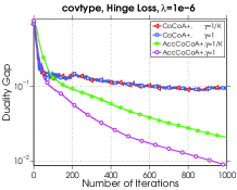
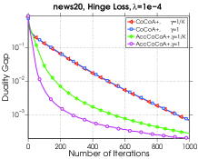
Refer to caption
Refer to caption
Refer to caption
Refer to caption
Refer to caption
Refer to caption
Figure 1: Duality gap as a function of iterations (top row) and elapsed time (bottom row) when solving hinge-loss SVM problems.

  
Refer to caption Refer to caption Refer to caption

Refer to caption
Refer to caption
Refer to caption
Figure 2: Duality gap as a function of iterations (top row) and elapsed time (bottom row) when solving hinge-loss SVM problems with different regularization values (λ𝜆\lambda) on the url dataset.

Figure 3 shows analogous results when the algorithms are employed to solve the Lasso problem in (1), for which increasing the regularization parameter λ1subscript𝜆1\lambda_{1} typically leads to more sparsity of the solution vector. The results indicate that the accelerated algorithm offers faster convergence of the sub-optimality gap to zero, especially for small values of λ1subscript𝜆1\lambda_{1}.

Refer to caption
Refer to caption
Refer to caption
Refer to caption
Figure 3: Sub-optimality gap as a function of iterations (top row) and elapsed time (bottom row) when solving Lasso problems. The choice of the regularizer value (λ1)subscript𝜆1(\lambda_{1}) are such that for the url dataset the density of the optimal solution is 5.3%percent5.35.3\%, while for the epsilon dataset the density is 13.56%percent13.5613.56\%.

We also ran experiments to demonstrate how the performance of AccCoCoA+ depends on the number of iterations (H𝐻H) that SDCA runs for solving each subproblem. Figure 5 shows that for larger H𝐻H the subproblems will be solved more accurately, and thus fewer outer iterations can be expected to reach a desired tolerance on the duality gap. However, in terms of running time, it is not always better to choice larger H𝐻H. For example, for the covtype dataset, choosing H=104𝐻superscript104H=10^{4} results in less time to reach a tolerance of 102superscript10210^{-2} than is needed when H=103𝐻superscript103H=10^{3} or H=105𝐻superscript105H=10^{5}. However, for the news20 dataset, the time required decreases with H𝐻H for all values considered in our experiments. The reason that this occurs is that d𝑑d is quite large in this dataset, which makes each round of communication quite time consuming. Therefore, by solving the subproblems more accurately (by running more iterations), one achieves a better balance between communication and computation.

Such a tradeoff between communication and computation can also be observed in Figure 5, where we compare how the values of H𝐻H can affect the convergence of the duality gap for the covtype and rcv_test datasets. The left two plots illustrate that to reach the same tolerance on the duality gap, the number of iterations can always be reduced by reaching a more accurate solution for each subproblem. However, the curves in the other two plots indicate that there is always a best value of H𝐻H that leads to fastest convergence with respect to running time.
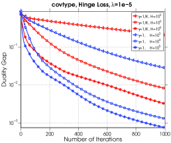
Refer to caption
Refer to caption
Refer to caption
Refer to caption
Figure 4: Comparison of performance for different inner iteration limits when σ=1Ksuperscript𝜎1𝐾\sigma^{\prime}=\frac{1}{K} and σ=1superscript𝜎1\sigma^{\prime}=1.

  
Refer to caption Refer to caption

Refer to caption
Refer to caption
Figure 5: Number of iterations and running time required to reach a tolerance of 103superscript10310^{-3} on the duality gap as the inner iteration limit (H𝐻H) is varied.

Our last experiment shows how AccCoCoA+ scales with the number of machines (K𝐾K). The results are shown in Figure 6. We set H=nK𝐻𝑛𝐾H=\frac{n}{K} for every K𝐾K to make sure that the same amount of data is utilized during each iteration of AccCoCoA+ across all K𝐾K machines. By doing so, it is also expected that each subproblem has been solved to similar accuracy, according to the complexity result of SDCA in [15]. The results show that when γ=1𝛾1\gamma=1, AccCoCoA+ takes almost the same amount of time regardless of how many machines are used, which demonstrates the better scaling properties it has than the γ=1K𝛾1𝐾\gamma=\frac{1}{K} case.

Refer to caption
Refer to caption
Figure 6: Running times on different numbers of machines K𝐾K.

5 Conclusion

We proposed and analyzed AccCoCoA+, an accelerated variant of CoCoA+ achieving the optimal 𝒪(1/t2)𝒪1superscript𝑡2\mathcal{O}(1/t^{2}) convergence rate. The method is robust to inaccurate subproblems both in theory and practice, and performs well in large-scale experiments. Our analysis provides constants in the convergence rate which are significantly tighter compared to those previously obtained for CoCoA+.

References

  • [1] Amir Beck and Marc Teboulle. A fast iterative shrinkage-thresholding algorithm for linear inverse problems. SIAM journal on imaging sciences, 2(1):183–202, 2009.
  • [2] Joseph K Bradley, Aapo Kyrola, Danny Bickson, and Carlos Guestrin. Parallel coordinate descent for l1-regularized loss minimization. arXiv:1105.5379, 2011.
  • [3] John Duchi, Elad Hazan, and Yoram Singer. Adaptive subgradient methods for online learning and stochastic optimization. The Journal of Machine Learning Research, 12:2121–2159, 2011.
  • [4] Celestine Dünner, Simone Forte, Martin Takáč, and Martin Jaggi. Primal-dual rates and certificates. arXiv:1602.05205, 2016.
  • [5] Olivier Fercoq and Peter Richtárik. Accelerated, parallel and proximal coordinate descent. SIAM Journal on Optimization, 25(4):1997–2023, 2015.
  • [6] Martin Jaggi, Virginia Smith, Martin Takác, Jonathan Terhorst, Sanjay Krishnan, Thomas Hofmann, and Michael I Jordan. Communication-efficient distributed dual coordinate ascent. In Advances in Neural Information Processing Systems, pages 3068–3076, 2014.
  • [7] Hongzhou Lin, Julien Mairal, and Zaid Harchaoui. A universal catalyst for first-order optimization. In Advances in Neural Information Processing Systems, pages 3366–3374, 2015.
  • [8] Ji Liu and Stephen J Wright. Asynchronous stochastic coordinate descent: Parallelism and convergence properties. SIAM Journal on Optimization, 25(1):351–376, 2015.
  • [9] Chenxin Ma, Jakub Konečnỳ, Martin Jaggi, Virginia Smith, Michael I Jordan, Peter Richtárik, and Martin Takáč. Distributed optimization with arbitrary local solvers. arXiv:1512.04039, 2015.
  • [10] Chenxin Ma, Virginia Smith, Martin Jaggi, Michael I Jordan, Peter Richtárik, and Martin Takáč. Adding vs. averaging in distributed primal-dual optimization. In 32th International Conference on Machine Learning, ICML 2015, 2015.
  • [11] Yu Nesterov. Gradient methods for minimizing composite functions. Mathematical Programming, 140(1):125–161, 2013.
  • [12] Yurii Nesterov. Introductory lectures on convex optimization: A basic course, volume 87. Springer Science & Business Media, 2013.
  • [13] Benjamin Recht, Christopher Re, Stephen Wright, and Feng Niu. Hogwild: A lock-free approach to parallelizing stochastic gradient descent. In Advances in Neural Information Processing Systems, pages 693–701, 2011.
  • [14] Shai Shalev-Shwartz and Tong Zhang. Accelerated mini-batch stochastic dual coordinate ascent. In Advances in Neural Information Processing Systems, pages 378–385, 2013.
  • [15] Shai Shalev-Shwartz and Tong Zhang. Stochastic dual coordinate ascent methods for regularized loss minimization. The Journal of Machine Learning Research, 14(1):567–599, 2013.
  • [16] Ohad Shamir, Nathan Srebro, and Tong Zhang. Communication efficient distributed optimization using an approximate newton-type method. arXiv:1312.7853, 2013.
  • [17] Virginia Smith, Simone Forte, Chenxin Ma, Martin Takáč, Michael I Jordan, and Martin Jaggi. CoCoA: A General Framework for Communication-Efficient Distributed Optimization. arXiv, 2016.
  • [18] Martin Takáč, Avleen Bijral, Peter Richtárik, and Nathan Srebro. Mini-batch primal and dual methods for svms. In In 30th International Conference on Machine Learning, ICML 2013, 2013.
  • [19] Martin Takáč, Peter Richtárik, and Nathan Srebro. Distributed mini-batch SDCA. arXiv:1507.08322, 2015.
  • [20] Tianbao Yang, Shenghuo Zhu, Rong Jin, and Yuanqing Lin. Analysis of distributed stochastic dual coordinate ascent. arXiv:1312.1031, 2013.
  • [21] Yuchen Zhang and Lin Xiao. Communication-efficient distributed optimization of self-concordant empirical loss. arXiv:1501.00263, 2015.
  • [22] Ciyou Zhu, Richard H Byrd, Peihuang Lu, and Jorge Nocedal. Algorithm 778: L-bfgs-b: Fortran subroutines for large-scale bound-constrained optimization. ACM Transactions on Mathematical Software (TOMS), 23(4):550–560, 1997.