Radiation-Reaction Force on a Small Charged Body to Second Order

Abstract

In classical electrodynamics, an accelerating charged body emits radiation and experiences a corresponding radiation-reaction force, or self force. We extend to higher order in the total charge a previous rigorous derivation of the electromagnetic self force in flat spacetime by Gralla, Harte, and Wald. The method introduced by Gralla, Harte, and Wald computes the self force from the Maxwell field equations and conservation of stress-energy in a limit where the charge, size, and mass of the body go to zero, and does not require regularization of a singular self field. For our higher order computation, an adjustment of the definition of the mass of the body is necessary to avoid including self energy from the electromagnetic field sourced by the body in the distant past. We derive the evolution equations for the mass, spin, and center-of-mass position of the body through second order. We derive, for the first time, the second-order acceleration dependence of the evolution of the spin (self torque), as well as a mixing between the extended body effects and the acceleration dependent effects on the overall body motion.

I Introduction

I.1 Status of our understanding of self force effects

Classical electrodynamics dictates that an accelerating charge emits radiation. This electromagnetic radiation carries energy and momentum, so conservation laws demand that the charge must experience a force. The force arises from the charge interacting with its own field, and is known as the ‘radiation-reaction force’ or ‘self force’. This phenomenon was first derived by Lorentz Lorentz (1915), and later confirmed by Abraham Abraham (1903) followed by Dirac Dirac (1938), each expanding and generalizing the results of the prior work.

Computing expressions for self forces is notoriously complicated, and there is an enormous literature on this field. The complexity arises in part because self forces describe back-reaction: as a charge accelerates, its radiation perturbs its motion, in turn altering the details of the radiation. Analytic methods are tractable in the regime in which the body is small compared to the characteristic lengthscales of the external fields. In this limit, the self force can be expanded order by order in the charge of the body. In this paper, we use the common nomenclature of referring to the Lorentz force as the leading order force, the leading correction to the Lorentz force as the ‘first order’ self force, and so on. Our understanding of radiation reaction in flat spacetime has been developed over most of a century Erber (1961); Mo and Papas (1971); Teitelboim (1971); Spohn (1999), culminating in the rigorous treatment of Gralla, Harte, and Wald Gralla et al. (2009)(henceforth GHW) who carefully analyzed a limit in which the charge, size, and mass of a body go to zero. The modern focus of the self force community is that of small masses in curved spacetime, for which Eric Possion’s review article offers a thorough introduction Poisson et al. (2011).

The self force is of great interest to modern astrophysics. Just as a charged particle interacts with its own field as it radiates electromagnetic waves, gravitating systems experience self forces from the emission of gravitational radiation. The gravitational waves produced by binary black hole inspirals and binary neutron star inspirals have been detected by LIGO LIGO Scientific Collaboration and Virgo Collaboration (2016, 2017), and similar binary inspirals are candidate signals for the future space-based detector LISA.

Making full use of the data from LISA will require an improved understanding of self force effects. The gravitational self force to leading order in the mass of the small body is referred to as the MiSaTaQuWa self force, and was first derived in Mino et al. (1997); Quinn and Wald (1997). More recent computations have extended these results to second order Rosenthal (2006); Pound (2014, 2015a); Detweiler (2012); Galley (2012a, b), and applied the self force to a gravitational inspiral, in order to compute or numerically evaluate the worldline and the resulting gravitational radiation. The computational strategies for evaluating worldlines and waveforms from gravitational self force are reviewed well in Wardell and Gopakumar (2015); Barack (2009). The techniques for computing leading order, or adiabatic, waveforms are now known. However, LISA data analysis will require post-adiabatic waveform predictions, which in turn will also require the subleading self force. This motivates a detailed understanding of the subleading self force.

Previous derivations of higher-order self forces for non-gravitational fields include those of Chad Galley Galley and Hu (2005) and Abraham Harte Harte (2015). Galley’s derivation Galley and Hu (2005) of the scalar self force uses an effective field technique to derive the self force to high order for monopolar charges. Harte has derived exact expressions for the self force of an extended charge distribution in an external field. The relation between Harte’s results and our work is somewhat involved and is discussed in Sec. III below.

I.2 The Gralla-Harte-Wald derivation method and its extension

In this paper, we derive the subleading order electromagnetic and scalar self forces acting on a small charged body moving in flat spacetime. The calculation is motivated by the importance of the gravitational self force, and is a model for the more complicated computation in the gravitational case. Although subleading self forces have previously been computed Pound (2012); Gralla (2012), ours is the first to describe extended body effects to subleading order. In addition to providing a model for the gravitational self force, our calculation may have direct application to systems with extremely strong electromagnetic fields, as discussed further below.

GHW introduce a one-parameter family of bodies with the property that as the parameter approaches zero, the mass, charge, and spatial extent of the body approach zero at the same rate. By considering various moments of the stress-energy conservation and charge conservation equations, integrated over a small region containing the body, they derive the first-order self force, mass evolution, and spin evolution equations.

Our calculation uses the GHW axioms with slight modifications, which are presented in full in section IV. However, we found it necessary to modify and refine the definitions of body parameters. GHW defined parameters such as the total mass-energy, angular momentum, and electromagnetic multipole moments in terms of integrals over a spacelike hypersurface perpendicular to the center of mass worldline. At second order, these definitions are problematic, and we replace them with body parameter definitions in terms of integrals over the future null cones of points on the center of mass worldline. With these definitions, the body parameters at a given time depend only on the body’s stress-energy and charge distribution at times within a light crossing time, not on the stress-energy or charge distribution in the distant past. This is because, in flat spacetime, the field at every point depends only on sources on that point’s past lightcone.

I.3 Discussion of results - applications in physical systems

Our results for the second order evolution of the body’s worldline, mass, and spin are given in Eqs. (77) - (80). They contain three types of terms: coupling of electromagnetic moments to the external field, self force terms that do not depend on the higher electromagnetic moments, and terms which describe a mixing between self-field and extended body effects. Our spin evolution equation contains a self-torque, which was not seen previously at lower orders. Our results also satisfy a consistency check obtained by comparing with some non-perturbative results of Harte Harte (2015).

As an illustrative special case, consider a body with vanishing spin, electromagnetic dipole, and quadrupole, moving in an external electromagnetic field $F^{(\text{ext})\mu\nu}$. The acceleration of the body can be written as [c.f. Eq. (V.4) below], in units with $c=1$,

$$a^{\mu}= \kappa F^{(\text{ext})\mu\lambda}u_{\lambda}+q\left\{\frac{2}{3}\kappa^{2}D_{\tau}F^{(\text{ext})\mu\lambda}u_{\lambda}+\frac{2}{3}\kappa^{3}\mathcal{P}^{\mu}{}_{\nu}F^{(\text{ext})\nu\lambda}F^{(\text{ext})}{}_{\lambda\sigma}u^{\sigma}\right\}$$

$$+q^{2}\bigg{\{}\frac{4}{9}\kappa^{3}D_{\tau}{}^{2}F^{(\text{ext})\mu\lambda}u_{\lambda}+\frac{8}{9}\kappa^{4}\mathcal{P}^{\mu}{}_{\kappa}F^{(\text{ext})\kappa\lambda}F^{(\text{ext})}{}_{\lambda\sigma}u^{\sigma}$$

$$\hskip 28.45274pt+\frac{4}{9}\kappa^{4}\mathcal{P}^{\mu}{}_{\kappa}F^{(\text{ext})\kappa\lambda}D_{\tau}F^{(\text{ext})}_{\lambda\sigma}u^{\sigma}+\frac{4}{9}\kappa^{5}\mathcal{P}^{\mu}{}_{\kappa}F^{(\text{ext})\kappa\rho}\mathcal{P}_{\rho\lambda}F^{(\text{ext})\lambda\sigma}F^{(\text{ext})}{}_{\sigma\omega}u^{\omega}\bigg{\}}+\mathcal{O}(q^{3}).$$ (1)

Here $u^{\mu}$ is the 4-velocity of the body, $a^{\mu}$ the 4-acceleration, $D_{\tau}\equiv u^{\mu}\nabla_{\mu}$, and $\mathcal{P}^{\mu}{}_{\nu}=\delta^{\mu}{}_{\nu}+u^{\mu}u_{\nu}$ is the projection tensor. Also, $q$ is the charge and $\kappa=q/m$ is the charge to mass ratio. The right hand side consists of an expansion in $q$ at fixed $\kappa$. The first term is the Lorentz force law, the second term is the reduced-order (see Sec. V.1 below) form of the Abraham-Lorentz-Dirac equation, and the third term is our new result.

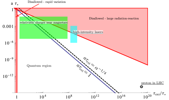
Figure 1: An illustration of the parameter space for radiation reaction for relativistic particles. The horizontal axis is the ratio $\tau_{\text{ext}}/\tau_{*}$, where $\tau_{\text{ext}}$ is the timescale over which the external field is varying, as measured in the instantaneous rest frame of the particle, and $\tau_{*}=q^{2}/m$, where $q$ is the charge and $m$ the mass of the particle. The vertical axis is $a\tau_{*}$, where $a$ is the acceleration due to the external field. The motion is relativistic in the region $a\tau_{\text{ext}}\gg 1$, in the upper right hand of the figure. Radiation reaction effects are large in the shaded regions where $\tau_{*}/\tau_{\text{ext}}\gtrsim 1$ or $a^{2}\tau_{\text{ext}}\tau_{*}\gtrsim 1$. These regions lie outside of the domain of validity of our analysis, and the second order self force is negligible except near the boundaries of these regions. In the region below and to the left of the dashed line, the radiation from the particle is not in a classical regime and our analysis does not apply. We show the location of protons in the Large Hadron Collider, protons in very high intensity lasers, and electrons in the high magnetic fields of magnetars.

We now turn to a discussion of the domain of validity of our results. Consider a charged body of mass $m$, and charge $q$, moving in an external field that imparts a characteristic acceleration $a$, as measured in the body’s instantaneous rest-frame. Suppose also that the field varies on some timescale or lengthscale $\tau_{\text{ext}}$, again as measured in the body’s instantaneous rest-frame. Then there are a number of conditions that must be satisfied for our analysis to be valid:

• Small multipole couplings: If the condition

  $$\mathcal{R}\ll\tau_{\text{ext}},$$ (2)

  is satisfied then the leading order couplings (dipole, quadrupole, and so on) will dominate.

• Weak radiation reaction: The energy radiated in a dynamical time must be small compared to the change in the body’s energy due to conservative effects. If this is violated then our derivation is no longer valid. In the non-relativistic region $a\tau_{\text{ext}}\ll 1$ this requires

  $$\frac{\tau_{*}}{\tau_{\text{ext}}}\ll 1$$ (3)

  where $\tau_{*}=q^{2}/m$. In the relativistic regime $a\tau_{\text{ext}}\gg 1$, the condition is instead

  $$a^{2}\tau_{\text{ext}}\tau_{*}\ll 1.$$ (4)

• Classical radiation regime: The energy radiated in a dynamical time must be large compared to the energy radiated per quantum, so that many quanta are emitted in a dynamical time. In the non-relativistic regime $a\tau_{\text{ext}}\ll 1$ the corresponding requirement is

  $$a\tau_{\text{ext}}\gg\alpha^{-1/2},$$ (5)

  where $\alpha=q^{2}/\hslash$, and the relativistic regime $a\tau_{\text{ext}}\gg 1$ it is

  $$a\tau_{\text{ext}}\gg\alpha^{-1/4}.$$ (6)

For elementary particles typically $\alpha\ll 1$ while for macroscopic charged bodies $\alpha\gg 1$.

Our derivation method employs a certain limiting procedure which automatically enforces the conditions (2),(3), and (4). The two dimensional parameter space of acceleration $a$ and external timescale $\tau_{\text{ext}}$ is illustrated in Fig 1. The solid line $a\tau_{\text{ext}}=1$ is the boundary between non-relativistic and relativistic motion; the lower left region is non-relativistic while the upper right is relativistic. The shaded regions on the left and at the top correspond to strong radiation reaction and lie outside our domain of validity, by (3) and (4). Our second order self force will be significant only near these boundaries. The region to the left of the dashed line is disallowed since the radiation is not classical, by (6) (assuming an elementary particle so that $\alpha\ll 1$). Also shown on the plot are some illustrative examples:

• A proton at the Large Hadron Collider, for which $a\sim 3\cdot 10^{12}\,\text{s}^{-1}$, $\tau_{\text{ext}}\sim 1.4\cdot 10^{-8}\,\text{s}$, $\tau_{*}\sim 6\cdot 10^{-27}\,\text{s}$. In this case we have $a^{2}\tau_{\text{ext}}\tau_{*}\sim 10^{-9}$, so higher order radiation reaction effects are negligible. Lead ions in the LHC experience a similar acceleration, and have a $\tau_{*}$ almost two orders of magnitude larger, $\tau_{*}\sim 2\cdot 10^{-25}\,\text{s}$, so the scale of effect is $a^{2}\tau_{\text{ext}}\tau_{*}\sim 10^{-8}$.

• For high-intensity laser systems with intensities in the range $10^{19}\,\text{W}/\text{cm}^{2}-10^{22}\,\text{W}/\text{cm}^{2}$ Kumar et al. (2013); Berezhiani et al. (2008); Chen et al. (2011), the acceleration scale for a proton is then in the range $a\sim 10^{17}\,\text{s}^{-1}-10^{21}\,\text{s}^{-1}$, and using $\tau_{\text{ext}}\sim 10^{-16}\,\text{s}$ and $\tau_{*}\sim 6\cdot 10^{-23}\,\text{s}$ gives $a^{2}\tau_{\text{ext}}\tau_{*}$ in the range $10^{-8}$-$10^{0}$. At the upper end of this range, second order radiation reaction effects could become significant. Krueger and Bovyn (1976)

• Turning to astrophysics, the magnetic fields near certain neutron stars, referred to as “magnetars”, can be extremely large, $B\sim 10^{8}-10^{11}\text{T}$. At the high end of this range, higher order self force effects could easily become large even for slowly moving particles.

II Motion of a finite body coupled to an external field

In this section, we consider a finite extended body moving in an external field in flat spacetime. We will review the governing equation, the non-perturbative definition of the body parameters. In the following sections we will review the non-perturbative equations of motion for the body moments, and specialize to the limit of a small body to obtain explicit results.

II.1 Governing equations

The system we are considering is a finite, extended, charged body coupled to an external field in flat spacetime. The extended body is described by a matter stress-energy tensor $T^{\mu\nu}_{M}$, which we assume is smooth and which vanishes outside a world tube of compact spatial support. We will consider both electromagnetic and scalar self forces.

The coupling to either type of field is governed by the body’s charge, which is described by a charge current density $j^{\mu}$ such that $\nabla_{\mu}j^{\mu}=0$ (electromagnetic case), or a scalar charge density $\rho$ (scalar case). We assume that the charge current or density functions are also smooth and of compact spatial support. These fields obey the standard inhomogeneous wave equations for the respective type of field:

$$\qquad\qquad\nabla_{[\mu}F_{\lambda\sigma]} =0,$$ (7a)

$$\qquad\qquad\nabla^{\mu}F_{\mu\nu} =4\pi j_{\nu}\qquad(\text{E\&M case}),$$ (7b)

and

$$\qquad\qquad\nabla_{\mu}\nabla^{\mu}\Phi=-4\pi\rho\qquad(\text{scalar case}).$$ (8)

The total stress-energy tensor $T_{\mu\nu}$ is given by the sum of the matter contribution $T_{M\,\mu\nu}$ and the field contribution $T_{F\,\mu\nu}$. This stress energy contribution for the electromagnetic field is

$$\qquad\qquad 4\pi T_{F\,\mu\nu}=F_{\mu\lambda}F^{\lambda}{}_{\nu}-\frac{1}{4}g_{\mu\nu}F_{\sigma\lambda}F^{\sigma\lambda},$$ (9)

or, for the scalar field, is

$$\qquad\qquad 4\pi T_{F\,\mu\nu}=\nabla_{\mu}\Phi\nabla_{\nu}\Phi-\frac{1}{2}g_{\mu\nu}\nabla_{\lambda}\Phi\nabla^{\lambda}\Phi.$$ (10)

We assume that this total stress-energy is conserved:

$$\nabla_{\mu}\left(T_{\text{M}}^{\mu\nu}+T_{\text{F}}^{\mu\nu}\right)=0.$$ (11)

We choose to divide the field into an external field $F^{(\text{ext})\mu\nu}$ (Scalar: $\Phi^{(\text{ext})}$), and a self field $F^{(\text{self})\mu\nu}$ (Scalar: $\Phi^{(\text{self})}$) which is the retarded solution to the field equations (7) or (8) with the given source. The external field may be expressed as, for the electromagnetic case,

$$\qquad\qquad F^{(\text{ext})}{}_{\mu\nu}=F_{\mu\nu}-F^{(\text{self})}{}_{\mu\nu},$$ (12)

or, for the scalar case,

$$\quad\qquad\qquad\Phi^{(\text{ext})}=\Phi-\Phi^{(\text{self})}.$$ (13)

Inserting the decompositions (12),(13) into the quadratic expressions (9),(10) for the field stress energy tensor, we find following GHW that the field stress energy can be expressed as the sum of three terms:

$$T_{\text{F}}^{\mu\nu}=T^{\mu\nu}_{(\text{self})}+T^{\mu\nu}_{(\text{cross})}+T^{\mu\nu}_{(\text{ext})}.$$ (14)

Here $T^{\mu\nu}_{(\text{self})}$ is quadratic in the self field, $T^{\mu\nu}_{(\text{ext})}$ is quadratic in the external field, and $T^{\mu\nu}_{(\text{cross})}$ is a cross term which depends on both the self field and the external field.

In the following subsection we will discuss the definition of body parameters such as mass, momentum, and spin. For those definitions, we will use the sum of the matter and self stress energy tensors,

$$T^{\mu\nu}=T_{\text{M}}^{\mu\nu}+T_{(\text{self})}^{\mu\nu},$$ (15)

excluding the cross and external contribution, following GHW. The conservation of stress-energy (11) can be rewritten in terms of this quantity as:

$$\nabla_{\mu}T^{\mu\nu}=F^{(\text{ext})\nu\mu}j_{\mu}\qquad\text{(E\&M case)},$$ (16a)

$$\nabla_{\mu}T^{\mu\nu}=\Phi^{(\text{ext});\nu}\rho\qquad\text{(scalar case)}.$$ (16b)

The motivation for choosing the definition (15) for the body parameter definitions is that in the limit when the body becomes small, the fields $T^{\mu\nu}$, $j^{\mu}$, and $\rho$ vary over the small body lengthscale, while the external fields $F^{(\text{ext})\mu\nu}$ and $\Phi^{(\text{ext});\mu}$ vary only on a longer lengthscale set by the external field.

The only equations that are needed for our derivation of the self force are the field equations (7) and (8), the stress energy conservation equation in the form (16), and the definition of the self-field as the retarded field.

II.2 Non-perturbative definition of body parameters: the Dixon-Harte formalism

We now turn to a discussion of the definition of body parameters for a finite body, including the body’s mass, momentum, spin, and choice of representative worldline.

For a conserved stress energy tensor $T^{\mu\nu}$ in flat spacetime of compact spatial support, there is a natural choice of momentum and spin, namely

$$P_{(\text{Isolated})}^{\mu}= \int_{\Sigma}T^{\mu\nu}d\Sigma_{\nu},$$ (17a)

$$S_{(\text{Isolated})}^{\mu\nu}(z^{\mu})= 2\int_{\Sigma}(x-z)^{[\mu}T^{\nu]\lambda}d\Sigma_{\lambda},$$ (17b)

where $\Sigma$ is any spacelike hypersurface. The center of mass worldline is then the set of points $z^{\mu}$ which satisfy

$$S_{(\text{Isolated})}^{\mu\nu}(z^{\mu})P_{(\text{Isolated})\nu}=0.$$ (18)

Equation (18) is known as a spin supplementary condition, and generalizations of this condition will be discussed below.

However, this treatment is not applicable to our present context for two reasons:

• First, the stress-energy tensor (15) that we wish to use in the definitions is not conserved, instead there is a forcing term from the external field on the right hand side of Eqs. (16). Hence, the expressions (17) will no longer be independent of the choice of hypersurface $\Sigma$, and a specific choice of hypersurface $\Sigma$ will be required. This will be discussed further below.

• Second, the stress energy term (15) that we will use does not have compact spatial support, due to the self field contribution. Hence, there is no guarantee that the expressions (17) are convergent and well defined. The convergence of these integrals is discussed further below.

There exists a general, fully non-perturbative set of definitions of worldlines, electromagnetic moments, and stress-energy moments of an extended body. These definitions were introduced by Dixon Dixon (1970a, b) in the context of curved spacetime, and extended by Harte Harte (2015). We follow the Dixon-Harte framework and definitions, with some modifications that we discuss below. The remainder of this section reviews those aspects of the Dixon-Harte framework that are most important for our derivation.

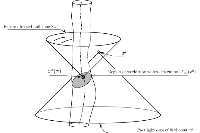
Figure 2: An illustration of our definitions of total momentum and spin of an extended body. The body is confined to the world tube shown, but is coupled to a long range field (scalar or electromagnetic) that extends beyond the worldtube. Given a representative worldline $z^{\mu}(\tau)$, shown as a dashed line, we define momentum and spin by integrating over future null cones $\Sigma_{\tau}$ of points on the worldline. The field stress energy tensor at a point $x^{\tilde{\mu}}$ on such a null cone will depend on the sources in the intersection of its past lightcone with the worldtube, shaded in gray. This region is confined to within the region of the worldtube consisting of times $\tau^{\prime}$ with $|\tau-\tau^{\prime}|$ smaller than a light-crossing time.

Before discussing the definitions of body parameters, we review the covariant bitensor formalism Poisson et al. (2011). We work in flat spacetime, but we will be using non-Lorentzian coordinates. We will denote by $x^{\tilde{\mu}}$ a field point off the worldline, and we use tilded indices for tensors at such points. We will denote by $z^{\mu}(\tau)$ a point on the worldline (figure 2), and use normal (untilded) indices for the tensors at such points. General bitensors are functions of both $z^{\mu}$ and $x^{\tilde{\mu}}$, and can have one or more indices of either type.

An important set of bitensors are Synge’s worldfunction $\sigma(x,z)$ and its derivatives. Synge’s worldfunction is defined only for pairs of points that are sufficiently close that there exists a unique geodesic that joins them. For this unique geodesic, $\sigma(x,z)$ measures the half geodesic distance squared between the two points. It is negative for timelike separated points, positive for spacelike separated points, and zero for null-related points. The first covariant derivative of Synge’s worldfunction can be used to define a covariant version of a position vector $\sigma_{\mu}(x,z)\equiv\nabla_{\mu}\sigma(x,z)$, where the derivative is with respect to $z$. We will also find useful the second derivatives, $\sigma^{\mu}{}_{\lambda}(x,z)\equiv\nabla_{\lambda}\nabla^{\mu}\sigma$ and $\sigma^{\tilde{\mu}}{}_{\lambda}\equiv\nabla^{\tilde{\mu}}\nabla_{\lambda}\sigma$.

In the Dixon-Harte framework, one chooses a worldline $z^{\alpha}(\tau)$ for the body, where $\tau$ is a parameter that need not be proper time, and a choice of a unit vector $n^{\alpha}(\tau)$ along the worldline with $n_{\alpha}(d/d\tau)^{\alpha}=-1$. The formalism supplies conditions that eventually determine the worldline and parameterization. Given these choices, one defines a foliation of spacetime by hypersurfaces $\Sigma_{\tau}$ as follows. Each hypersurface is labeled by the parameter $\tau$ at which it intersects the worldline, so $z^{\alpha}(\tau)\in\Sigma_{\tau}$, and is generated by geodesics starting on the worldline that are orthogonal to $n^{\alpha}$.

The Dixon-Harte definitions of the momentum and spin of an extended body are

$$P_{\mu}^{\text{D}}(\tau)= \int_{\Sigma_{\tau}}d\Sigma_{\tilde{\mu}}(x)T_{M}^{\tilde{\mu}\tilde{\nu}}(x)K_{\tilde{\nu}\mu}(x,z_{\tau}),$$ (19a)

$$S_{\mu\nu}^{\text{D}}(\tau)= 2\int_{\Sigma_{\tau}}d\Sigma_{\tilde{\mu}}(x)T_{M}^{\tilde{\mu}\tilde{\nu}}(x)H_{\tilde{\nu}[\mu}(x,z_{\tau})\sigma_{\nu]}(x,z_{\tau}),$$ (19b)

where

$$H^{\tilde{\mu}}{}_{\nu}= -\left(\sigma^{\nu}{}_{\tilde{\mu}}\right)^{-1},$$ (20a)

$$K^{\tilde{\mu}}{}_{\nu}= H^{\tilde{\mu}}{}_{\lambda}\sigma^{\lambda}{}_{\nu}.$$ (20b)

In flat spacetime, these definitions reduce to:

$$P_{D}^{\mu}(\tau)= \int_{\Sigma_{\tau}}d\Sigma_{\tilde{\mu}}(x^{\tilde{\lambda}})T_{M}^{\tilde{\mu}\tilde{\nu}}(x^{\tilde{\lambda}})g_{\tilde{\nu}}{}^{\mu}(x^{\tilde{\lambda}},z^{\lambda}(\tau)),$$ (21a)

$$S_{D}^{\mu\nu}(\tau)= 2\int_{\Sigma_{\tau}}d\Sigma_{\tilde{\mu}}(x^{\tilde{\lambda}})T_{M}^{\tilde{\mu}\tilde{\nu}}(x^{\tilde{\lambda}})g_{\tilde{\nu}}{}^{[\mu}(x^{\tilde{\lambda}},z^{\lambda})\sigma^{\nu]}(x^{\tilde{\lambda}},z^{\lambda}),$$ (21b)

where $g_{\mu\tilde{\nu}}\equiv-\sigma_{\mu\tilde{\nu}}$ is the parallel propagator bitensor in flat spacetime.

We modify the Dixon-Harte framework in the following ways.

• We specialize the parameter $\tau$ to be the proper time.

• We dispense with the unit vector $n^{\alpha}(\tau)$.

• We use the stress energy tensor $T^{\mu\nu}$ of Eq. (15) instead of the matter stress energy tensor $T_{M}^{\mu\nu}$.

• We use null hypersurfaces $\Sigma_{\tau}$ that are generated by the set of future null geodesics starting at worldline point $z^{\alpha}(\tau)$. This family of null hypersurfaces foliates the convex normal neighborhood of the worldline, which covers the entire manifold for the flat spacetime case we consider in this paper.

Our definitions are then

$$P_{B}^{\mu}(\tau)= \int_{\Sigma_{\tau}}d\Sigma_{\tilde{\mu}}(x^{\tilde{\lambda}})T^{\tilde{\mu}\tilde{\nu}}(x^{\tilde{\lambda}})g_{\tilde{\nu}}{}^{\mu}(x^{\tilde{\lambda}},z^{\lambda}(\tau)),$$ (22a)

$$S_{B}^{\mu\nu}(\tau)= 2\int_{\Sigma_{\tau}}d\Sigma_{\tilde{\mu}}(x^{\tilde{\lambda}})T^{\tilde{\mu}\tilde{\nu}}(x^{\tilde{\lambda}})g_{\tilde{\nu}}{}^{[\mu}(x^{\tilde{\lambda}},z^{\lambda})\sigma^{\nu]}(x^{\tilde{\lambda}},z^{\lambda}),$$ (22b)

Here the subscript $B$ denotes “bare”; these definitions will be replaced by renormalized momentum and spin in Sec. IV.6 below.

The motivations for our choice of foliation of future null cones are as follows. The integrals (17) contain a contribution from the stress energy tensor of the self field from Eq. (15). That self field, evaluated at a point $x$ on the hypersurface $\Sigma_{\tau}$ over which one integrates, in turn depends on the body’s charge distribution on the past light cone of $x$. When one uses a spacelike hypersurface $\Sigma_{\tau}$, the dependence on the body’s charge distribution extends into the distant past, as one takes $x$ further and further out on the spacelike hypersurface. By contrast, for a future null cone, $\Sigma_{\tau}$, the dependence on the body’s charge distribution is limited to times within a light-crossing time of $\tau$, as illustrated in figure (2). In addition, we show in Appendix A that the integrals (22) are well defined and finite when the hypersurfaces $\Sigma_{\tau}$ are chosen to be future null cones.

There are three choices we have alluded to in the above definition of momentum and spin: the worldline $z(\tau)$ (which is fixed by the spin supplementary condition), the choice (15) of body stress-energy tensor, and the choice of the hypersurface of integration. As we have argued, not all choices give rise to physically acceptable definitions. Within those that do there is considerable freedom. This freedom corresponds to different ways of describing a given dynamical system. Different choices will give rise to different forms of the laws of motion, but will not change any physical predictions.

We also define the bare rest mass $m_{B}$ by

$$m_{B}^{2}\equiv-P_{B}^{\mu}P_{B\,\mu}.$$ (23)

We define the 4-velocity in the usual way as $u^{\mu}(\tau)=dz^{\mu}/d\tau$, with $u^{\mu}u_{\mu}=-1$, and note that

$$P_{B}^{\mu}\neq m_{B}u^{\mu},$$ (24)

beyond leading order.

The definitions (22) are valid for any choice of worldline $z_{\tau}$. To pick out a unique worldline one must specify a spin supplementary condition Dixon (1970a, b), which takes the generic form

$$S_{B}^{\mu\nu}(\tau)\omega_{\nu}=0,$$ (25)

where $\omega_{\nu}$ is some vector field defined on the worldline. Such a spin supplementary condition defines a center of mass worldline Kyrian and Semer?k (2007) Costa et al. (2016). Our the spin supplementary condition is defined in terms of a renormalized spin $S^{\mu\nu}$, which we define in Eq. (63) below. Our spin supplementary condition is

$$S^{\mu\nu}u_{\nu}=0,$$ (26)

which reduces at leading order in the size and mass of the body to the condition (25) with $\omega_{\nu}=u_{\nu}$.

II.3 Electromagnetic multipole moments

We now turn to a discussion of electromagnetic multipole moments. We define the total (conserved) bare charge $q_{B}$, charge moment $\mathcal{J}^{\mu}_{B}$, dipole $Q_{B}^{\mu\nu}$, and quadrupole $Q_{B}^{\mu\nu\rho}$ of the body to be

$$q_{B}(\tau)=q_{B}= \int_{\Sigma_{\tau}}d\Sigma_{\tilde{\nu}}j^{\tilde{\nu}},$$ (27a)

$$\mathcal{J}_{B}^{\mu}(\tau)= \int_{\Sigma_{\tau}}d\Sigma_{\tilde{\nu}}g^{\tilde{\nu}}{}_{\lambda}u^{\lambda}j^{\tilde{\mu}}g_{\tilde{\mu}}{}^{\mu},$$ (27b)

$$Q_{B}^{\mu\nu}(\tau)= -\int_{\Sigma_{\tau}}d\Sigma_{\tilde{\nu}}g^{\tilde{\nu}}{}_{\lambda}u^{\lambda}j^{\tilde{\mu}}g_{\tilde{\mu}}{}^{\mu}\sigma^{\nu},$$ (27c)

$$Q_{B}^{\mu\nu\rho}(\tau)= \int_{\Sigma_{\tau}}d\Sigma_{\tilde{\nu}}g^{\tilde{\nu}}{}_{\lambda}u^{\lambda}j^{\tilde{\mu}}g_{\tilde{\mu}}{}^{\mu}\sigma^{\nu}\sigma^{\rho}.$$ (27d)

In these expressions, the arguments of all the bitensors $g^{\tilde{\nu}}{}_{\lambda}$, $\sigma^{\nu}$, etc. are $(x,z(\tau))$, while the argument of $j^{\tilde{\mu}}$ is $(x)$. The definition (27c) has a minus sign due to the properties of Synge’s worldfunction ($g_{\mu}{}^{\tilde{\nu}}\sigma^{\mu}=-\sigma^{\tilde{\nu}}$).

For the Dixon moments Dixon (1970b) defined in terms of a spacelike hypersurface generated by geodesics orthogonal to $n^{\mu}(\tau)$, the bitensor $\sigma^{\mu}(x,z(\tau))$ is orthogonal to $n^{\mu}(\tau)$ for all $x$ in $\Sigma_{\tau}$, and hence all of the charge moments are orthogonal to $n^{\mu}$ in all indices following the first index:

$$Q_{D}^{\mu\nu}n_{\mu}=Q_{D}^{\mu\nu\rho}n_{\mu}=Q_{D}^{\mu\nu\rho}n_{\rho}=0.$$ (28)

Since we integrate over future-directed null cones, there is no such orthogonality condition for our moments (27). In addition, our dipole (27c) contains both a symmetric and an antisymmetric part, unlike the case for the standard definition which includes an explicit antisymmetrization.

The number of independent components of the electromagnetic dipole (27c) and quadrupole (27d) are nominally 16 and 40, respectively. When charge conservation is imposed in Sec. VI.1, we shall see that these reduce to 10 and 22. However, these are still larger than the number of degrees of freedom for the standard definitions of the electromagnetic dipole and quadrupole, which are 6 and 14. Our bare electromagnetic moments (27) are convenient for our derivation in Sec. VI. However, we shall express our final results for the equations of motion in terms of a set of renormalized, projected moments, defined in Sec. IV.6, which have the standard number of degrees of freedom.

II.4 Scalar multipole moments

For the scalar case, we define an analogous set of bare moments, based on integrals over the scalar source $\rho$,

$$q_{SB}(\tau)= \int_{\Sigma_{\tau}}d\Sigma_{\tilde{\nu}}u^{\tilde{\nu}}\rho,$$ (29a)

$$Q_{SB}^{\mu}(\tau)= -\int_{\Sigma_{\tau}}d\Sigma_{\tilde{\nu}}g^{\tilde{\nu}}{}_{\lambda}u^{\lambda}\rho\sigma^{\mu},$$ (29b)

$$Q^{\mu\nu}_{SB}(\tau)= \int_{\Sigma_{\tau}}d\Sigma_{\tilde{\nu}}g^{\tilde{\nu}}{}_{\lambda}u^{\lambda}\rho\sigma^{\mu}\sigma^{\nu}.$$ (29c)

All other details regarding the absence of an orthogonality condition, and the comparison to standard multipoles are similar to those for the electromagnetic multipoles. Here the subscript $S$ denotes “scalar” and $B$ denotes “bare”.

The multipole moments (27) and (29) that we are defining are non-standard. However, they contain the same information as standard multipole moments which are defined in terms of integrals over spacelike hypersurfaces. Some insight into the relation between the two sets of moments can be obtained by considering the leading order expansion for $\Phi$ in terms of its source $\rho$ in a Lorentz frame $(t,x^{i})$:

$$\Phi(t,r,n^{i})=\frac{1}{r}\int d^{3}y\rho(t-r+{\bf n}\cdot{\bf y},{\bf y})+\mathcal{O}\left(\frac{1}{r^{2}}\right),$$ (30)

where

$$r=|{\bf x}|\hskip 28.45274pt\text{and}\hskip 28.45274ptn^{i}=\frac{x^{i}}{r}.$$ (31)

Taylor expanding the density about the retarded time $t-r$ gives the usual multipole expression

$$\Phi(t,r,n^{i})=\frac{1}{r}\sum_{k=0}^{\infty}\bigg{[}\frac{1}{k!}n^{i_{1}}\dots n^{i_{k}}\int d^{3}yy^{i_{1}}\dots y^{i_{k}}\rho^{(k)}(t-r,{\bf y})\bigg{]}+\mathcal{O}\left(\frac{1}{r^{2}}\right),$$ (32)

where $\rho^{(k)}$ denotes the $k^{\text{th}}$ time derivative. Taylor expanding instead about $r-t+y$ yields

$$\Phi(t,r,n^{i})=\frac{1}{r}\sum_{k=0}^{\infty} \left[\frac{1}{k!}\int d^{3}y(n^{i}y^{i}-y)^{k}\rho^{(k)}(t-r+y,{\bf y})\right]+\mathcal{O}\left(\frac{1}{r^{2}}\right),$$ (33)

which now involves integral over the future null cones. The integrals that appear in (33) are precisely time derivatives of our nonstandard multipoles (29)

III Non-perturbative equations of motion

This paper focuses primarily on a perturbative expansion of the self force. It is informative, though, to consider the extent to which exact computations can be used to determine radiation-reaction effects. In this section, we derive an exact law of motion for extended bodies, which is used indirectly in our derivation in the remainder of the paper. Our exact law is a modification of an exact law of motion due to Harte Dixon (1970a); Harte (2015), which we review. We use Harte’s result to perform a consistency check of our results in Sec.VI below.

III.1 Equation of motion for bare momentum

First, we define a generalized momentum $P_{\tau}(\vec{\xi})$ as a linear map on vector fields $\xi^{\tilde{\mu}}$ via

$$P_{\tau}(\vec{\xi})=\int_{\Sigma_{\tau}}T^{\tilde{\mu}\tilde{\nu}}\xi_{\tilde{\mu}}d\Sigma_{\tilde{\nu}}.$$ (34)

Here, as before, we choose the surface $\Sigma_{\tau}$ of integration to be future-directed null cones. When we specialize $\vec{\xi}$ to be a Killing vector field $\xi_{\tilde{\mu}}=g_{\tilde{\mu}}{}^{\mu}$ or $\xi_{\tilde{\mu}}=2g_{\tilde{\mu}}{}^{[\sigma}\sigma^{\nu]}$, the resulting quantities (34) yields the definitions (22) of linear momentum and spin Harte (2015).

To compute the time derivative of this generalized momentum, we use the general identity Harte (2015)

$$\frac{d}{d\tau}\int_{\Sigma_{\tau}}v^{\tilde{\mu}}d\Sigma_{\tilde{\mu}}=\int_{\Sigma_{\tau}}\nabla_{\tilde{\mu}}v^{\tilde{\mu}}m^{\tilde{\lambda}}d\Sigma_{\tilde{\lambda}}+\int_{\partial\Sigma_{\tau}}v^{\tilde{\mu}}m^{\tilde{\lambda}}dS_{\tilde{\mu}\tilde{\lambda}},$$ (35)

valid for any foliation $\Sigma_{\tau}$ and any vector field $v^{\tilde{\mu}}$. Here $m^{\tilde{\mu}}$ is any vector field that satisfies $m^{\tilde{\lambda}}(d\tau)_{\tilde{\lambda}}=1$, $dS_{\tilde{\mu}\tilde{\lambda}}=dS_{[\tilde{\mu}\tilde{\lambda}]}$ is the surface area element, and the second term of the right hand side should be interpreted as a limit of integrals over the boundaries of finite regions of $\Sigma_{\tau}$. Applying this identity with $v^{\tilde{\mu}}=T^{\tilde{\mu}\tilde{\nu}}\xi_{\tilde{\nu}}$ gives

$$\frac{d}{d\tau} P_{\tau}(\vec{\xi})=\int_{\Sigma_{\tau}}\nabla_{\tilde{\mu}}T^{\tilde{\mu}\tilde{\nu}}\xi_{\tilde{\nu}}m^{\tilde{\lambda}}d\Sigma_{\tilde{\lambda}}+\frac{1}{2}\int_{\Sigma_{\tau}}T^{\tilde{\mu}\tilde{\nu}}(\mathcal{L}_{\xi}g)_{\tilde{\mu}\tilde{\nu}}m^{\tilde{\lambda}}d\Sigma_{\tilde{\lambda}}-\int_{\partial\Sigma_{\tau}}T^{(\text{self})\tilde{\nu}\tilde{\mu}}\xi_{\tilde{\mu}}m^{\tilde{\lambda}}dS_{\tilde{\nu}\tilde{\lambda}},$$ (36)

In the last term, we’ve removed the matter contribution to the stress energy tensor, since it has compact spatial support and so does not contribute to the boundary integral in the asymptotic limit. Using Eq. (16a) we can rewrite the first term of (36) in terms of the external field. Specializing to Killing vector fields, for which the second term vanishes, gives

$$\frac{d}{d\tau}P_{\tau}(\vec{\xi})= \int_{\Sigma_{\tau}}\left(F^{(\text{ext})\tilde{\mu}\tilde{\nu}}\xi_{\tilde{\mu}}j_{\tilde{\nu}}\right)m^{\tilde{\lambda}}d\Sigma_{\tilde{\lambda}}-\int_{\partial\Sigma_{\tau}}T^{(\text{self})\tilde{\mu}\tilde{\nu}}\xi_{\tilde{\nu}}m^{\tilde{\lambda}}dS_{\tilde{\mu}\tilde{\lambda}}.$$ (37)

To obtain an explicit equation of motion for the worldline, Eq. (37) must be supplemented by the spin supplementary condition (26) that determines the relationship between the 4-velocity $u^{\mu}=dz^{\mu}/d\tau$ of the worldline and the 4-momentum $P_{B}^{\mu}$. To incorporate this condition we proceed as follows. First, we write down the following identities that are valid for any choice of vector field $P_{B}^{\mu}$ along the worldline

$$m_{B}a^{\kappa}= a^{\kappa}\left(m_{B}+P_{B}^{\mu}u_{\mu}\right)+\mathcal{P}^{\mu}{}_{\lambda}D_{\tau}P_{B}^{\lambda}-\mathcal{P}^{\kappa}{}_{\nu}D_{\tau}\left(\mathcal{P}^{\nu}{}_{\lambda}P_{B}^{\lambda}\right),$$ (38a)

$$D_{\tau}m_{B}= D_{\tau}\left(m_{B}+P_{B}^{\mu}u_{\mu}\right)-u_{\mu}D_{\tau}P_{B}^{\mu}-a_{\mu}P_{B}^{\mu}.$$ (38b)

Here $D_{\tau}\equiv u^{\mu}\nabla_{\mu}$ is the covariant derivative along the worldline, $a^{\kappa}=D_{\tau}u^{\kappa}$ is the 4-acceleration, and

$$\mathcal{P}^{\mu}{}_{\lambda}=\delta^{\mu}{}_{\lambda}+u^{\mu}u_{\lambda}$$ (39)

is the projection tensor onto the space of vectors orthogonal to the 4-velocity. The second term in each of Eqs (38a), (38b) can be obtained from (37) with the choice $\xi_{\tilde{\mu}}=g_{\tilde{\mu}}{}^{\mu}$ and the replacement $d/d\tau\rightarrow D_{\tau}$. For the first and third terms, we use the general identity (35) specialized to

$$v^{\tilde{\mu}}=\sigma^{\mu}T^{\tilde{\mu}\tilde{\lambda}}n_{\tilde{\lambda}},$$ (40)

where $n_{\tilde{\lambda}}=-(d\tau)_{\tilde{\lambda}}$ is the null normal to the future null cone $\Sigma_{\tau}$. Using $\nabla_{\tilde{\mu}}\sigma^{\mu}=-g_{\tilde{\mu}}{}^{\mu}$, Eq. (16a), and the identity for any vector field $v^{\tilde{\mu}}$:

$$\int_{\Sigma_{\tau}}v^{\tilde{\mu}}d\Sigma_{\tilde{\mu}}=-\int_{\Sigma_{\tau}}v^{\tilde{\mu}}n_{\tilde{\mu}}m^{\tilde{\lambda}}d\Sigma_{\tilde{\lambda}},$$ (41)

we obtain an expression for the bare momentum:

$$P_{B}^{\mu}(\tau)= D_{\tau}\int_{\Sigma_{\tau}}\sigma^{\mu}T^{\tilde{\mu}\tilde{\lambda}}n_{\tilde{\lambda}}d\Sigma_{\tilde{\mu}}+\int_{\Sigma_{\tau}}\sigma^{\mu}\left[F^{(\text{ext})\tilde{\lambda}\tilde{\rho}}j_{\tilde{\rho}}-T^{\tilde{\mu}\tilde{\rho}}\nabla_{\tilde{\mu}}n_{\tilde{\rho}}m^{\tilde{\lambda}}\right]d\Sigma_{\tilde{\lambda}}-\int_{\partial\Sigma_{\tau}}\sigma^{\mu}m^{[\tilde{\lambda}}T^{\tilde{\mu}]\tilde{\rho}}n_{\tilde{\rho}}dS_{\tilde{\mu}\tilde{\lambda}}.$$ (42)

Using the method of Appendix A, one can show that the boundary term in (42) vanishes when we choose $\vec{m}=\partial/\partial\tau$ in the coordinates constructed in VI.1. The expression (42) can now be substituted into the right hand sides of Eqs. (38a) and (38b) to give explicit evolution equations for the worldline $z^{\mu}(\tau)$ and bare mass $m_{B}(\tau)$.

In Sec. V.2 below we will describe a limit in which the charge, mass, and size of the body all go to zero. In this limit, the right hand sides of Eqs. (37) and (42) can be expanded in terms of electromagnetic multipole moments discussed in Sec. II.3, thereby yielding the explicit form of the equation of motion in this limit. This calculation is carried out in Sec. VI. Some of our calculations will proceed directly by taking moments of the field equations (7) and (16), rather than using Eqs. (37) and (42).

III.2 Equation of motion for Harte’s momentum

We now describe an alternative non-perturbative equation of motion for the momentum of extended charged bodies in Minkowski spacetime, due to Harte Harte (2015). It is based on Harte’s generalized momentum,

$$P_{H\,\tau}(\vec{\xi})=\int_{\Sigma_{\tau}}T_{M}^{\tilde{\mu}\tilde{\nu}}\xi_{\tilde{\mu}}d\Sigma_{\tilde{\nu}}+E_{\tau}(\vec{\xi}).$$ (43)

Here the first term coincides with our bare generalized momentum (34), but omits the self-field contribution. The second term $E_{\tau}(\vec{\xi})$ is a kind of self-field contribution, and is given by Eq.(184) of Ref. Harte (2015). It is a double integral over spacetime that is quadratic in the source $j^{\tilde{\mu}}$, involves a Greens function, and depends on the source only at times $\tau^{\prime}$ that are within a light-crossing time of $\tau$. Its explicit form will not be needed in what follows.

Harte’s non-perturbative equation of motion is

$$\frac{d}{d\tau}P_{H\,\tau}(\vec{\xi})=\int_{\Sigma_{\tau}}d\Sigma_{\tilde{\nu}}m^{\tilde{\nu}}\left(F^{\tilde{\lambda}\tilde{\rho}}-F_{S}^{\tilde{\lambda\tilde{\rho}}}\right)\xi_{\tilde{\lambda}}j_{\tilde{\rho}},$$ (44)

for Killing vectors $\vec{\xi}$, where $F_{S}^{\tilde{\lambda}\tilde{\rho}}$ is the average of retarded and advanced self-fields. Harte incorporates the spin-supplementary condition by solving explicitly for the relationship between the 4-velocity and momentum with a choice of parameter $\tau$ which differs from proper time. We find it more convenient to proceed instead as described above using the general identity (38) and choosing $\tau$ to be proper time.

We shall make use of Harte’s equation (44) as a partial consistency check of our results. By subtracting Eqs.(36) and (44), we obtain

$$\int_{\Sigma_{\tau}}d\Sigma_{\tilde{\nu}}m^{\tilde{\nu}}F_{R}^{\tilde{\lambda}\tilde{\rho}}\xi_{\tilde{\lambda}}j_{\tilde{\rho}} +\int_{\partial\Sigma_{\tau}}T^{(\text{self})\tilde{\mu}\tilde{\nu}}\xi_{\tilde{\nu}}m^{\tilde{\lambda}}dS_{\tilde{\mu}\tilde{\lambda}}=\left(\begin{array}[]{c}\text{Some total}\\ \text{time derivative}\end{array}\right),$$ (47)

where $F_{R}^{\tilde{\lambda}\tilde{\rho}}$ is the radiative self-field, one half the retarded field minus one half the advanced field. We compute the left hand side of explicitly in terms of our multipole expansion and verify that it is a total time derivative at each order in the expansion; see Secs. VI.4.2 and VI.5.2 below.

IV The point particle limit in the electromagnetic case

IV.1 One parameter families of solutions: the Gralla-Harte-Wald axioms

We will consider a small charged body interacting with an external electromagnetic field. To describe the limit in which the body becomes very small, we consider a one-parameter family of solutions of the field equations for the body, labeled by a dimensionless parameter $\lambda$. Following GHW, we impose the following axioms on the family of solutions. The axioms enforce that the mass and charge of the body go to zero as the size goes to zero.

Axiom 1

There exists a one-parameter family of fields consisting of the Maxwell tensor $F_{\mu\nu}(\lambda,x^{\mu})$, the charge current density $j^{\mu}(\lambda,x^{\mu})$, and the stress-energy tensor $T_{M}^{\mu\nu}(\lambda,x^{\mu})$, which satisfy the Maxwell, charge current conservation and stress-energy conservation equations:

$$\nabla^{\nu}F_{\mu\nu}(\lambda,x^{\mu})= 4\pi j_{\nu}(\lambda,x^{\mu}),$$ (48a)

$$\nabla_{[\mu}F_{\nu\lambda]}= 0,$$ (48b)

$$\nabla_{\mu}j^{\mu}(\lambda,x^{\mu})= 0,$$ (48c)

$$\nabla_{\mu}T^{\mu\nu}(\lambda,x^{\mu})= 0,$$ (48d)

where $T^{\mu\nu}\equiv T^{\mu\nu}_{M}+T^{\mu\nu}_{F}$, and $T^{\mu\nu}_{F}$ is given by (9). These fields are defined on the open interval $0<\lambda<\lambda_{0}$, for some $\lambda_{0}$.

Axiom 2

We assume there exist functions $\tilde{j}^{\mu}(\lambda,t,X^{i})$ and $\tilde{T}_{M}^{\mu\nu}(\lambda,t,X^{i})$ such that for some global Lorentz frame coordinates $(t,x^{i})$:

$$j^{\mu}(\lambda,t,x^{i})= \lambda^{-2}\tilde{j}^{\mu}\left(\lambda,t,\frac{x^{i}-z^{i}(\lambda,t)}{\lambda}\right),$$ (49a)

$$T_{M}^{\mu\nu}(\lambda,t,x^{i})= \lambda^{-2}\tilde{T}_{M}^{\mu\nu}\left(\lambda,t,\frac{x^{i}-z^{i}(\lambda,t)}{\lambda}\right),$$ (49b)

where $\tilde{j}^{\mu}$ and $\tilde{T}_{M}^{\mu\nu}$ are jointly smooth all of in their arguments, including at $\lambda=0$, and $z^{i}(\lambda,t)$ is the center-of mass worldline defined by (26).

Axiom 3

All of the fields $F_{\mu\nu}$, $j^{\mu}$, and $T_{\mu\nu}^{M}$ are jointly smooth in $x^{\mu}$ and $\lambda$ away from $\lambda=0$. There exists a worldtube $\mathcal{W}$ of compact spatial support such that the supports of $\tilde{j}^{\mu}$ and $\tilde{T}^{\mu\nu}_{M}$ lie inside $\mathcal{W}$ for all $\lambda$.

Axiom 4

The external field $F^{(\text{\emph{ext}})\mu\nu}$ defined by (12) is jointly smooth in $x^{\tilde{\mu}}$ and $\lambda$, including at $\lambda=0$.

IV.2 Discussion of and motivation for the axioms

As in GHW, the axioms 1-4 are intended to describe a family of physically reasonable charge current and stress-energy distributions, such that the limit $\lambda\rightarrow 0$ represents a pointlike object. At any finite $\lambda$, however, the object is nonsingular with smooth (in particular, non-distributional) sources and a finite self field. Our goal is to derive a set of ordinary differential equations that govern the motion of the object in the limit of small $\lambda$.

The axioms enforce a limit where the size $\mathcal{L}$ of the body is much smaller than the scale $\mathcal{L}_{\text{ext}}$ of variation of the external field $F^{(\text{ext})\mu\nu}$. Thus, there is a separation of scales

$$\mathcal{L}<<\mathcal{L}_{\text{ext}}.$$ (50)

One can think of the parameter $\lambda$ in our one parameter family of solutions as being the ratio $\mathcal{L}/\mathcal{L}_{\text{ext}}$, since the size of the body decreases linearly with $\lambda$, from Eqs. (49a) and (49b). As discussed by GHW, a crucial feature of the assumed one-parameter family is that the mass and charge of the body go to zero as $\lambda\rightarrow 0$, at the same rate as the size.

Our axioms are identical to those of GHW except for the status of the worldline. GHW assume the existence of a $\lambda$-independent worldline $z^{i}(t)$ for which a version of (49), with $z^{i}(\lambda,t)$ replaced by $z^{i}(t)$, is satisfied. By contrast, we define a one-parameter family of worldlines $z^{i}(\lambda,t)$ according to the general prescription described in Sec. II.2. The two approaches coincide at leading order, but at subleading order the $\lambda$-dependent worldline is more convenient.

Axiom 2 appears to violate Lorentz invariance by the choice of a specific Lorentz frame. However, if this assumption is satisfied in some Lorentz frame, it is satisfied in all Lorentz frames, so it does not violate Lorentz invariance.

IV.3 Consequence of axioms: the near zone and far zone limits

Following GHW, it is instructive to consider two different limits of $\lambda\rightarrow 0$ that give complementary descriptions of the interaction of the body with the external field.

The limit $\lambda\rightarrow 0$ at fixed rescaled coordinates

$$(T,X^{i})\equiv\left(t,\frac{x^{i}-z^{i}(t,\lambda)}{\lambda}\right),$$ (51)

describes the “near zone” limit. It describes what would be measured by observers at distances from the object of order the object’s size $\mathcal{L}$. In this limit, points with fixed global Lorentzian coordinates $x^{i}$ become more and more distant as $\lambda\rightarrow 0$. The lengthscale $\mathcal{L}_{\text{ext}}$ of the external field goes to infinity, while the size $\mathcal{L}$ of the body remains finite.

The limit $\lambda\rightarrow 0$ at fixed $(t,x^{i})$ describes the “far zone” limit. It describes what would be measured by observers at distances from the object of order $\mathcal{L}_{\text{ext}}$. In this limit, points at fixed rescaled coordinates $(T,X^{i})$ approach the worldline $x^{i}=z^{i}(0,t)$ as $\lambda\rightarrow 0$. In particular, the object’s size $\mathcal{L}\rightarrow 0$ as $\lambda\rightarrow 0$ at fixed $(t,x^{i})$.

The GHW axiom approach is closely related to the matched asymptotics method often used in gravitational calculations Poisson et al. (2011); Mino et al. (1997); Pound (2010); D’Eath (1975); Gralla and Wald (2008). The ‘near zone’ expressions are analogous to an expansion in positive powers of the radial coordinate, valid near the body, and the ‘far zone’ expressions are analogous to the expansions approximating the body as a pointlike source.

We now discuss the limiting behavior of the self-field as $\lambda\rightarrow 0$. The assumptions of subsection II.1 do not demand smoothness of the matter fields $j^{\mu}$ and $T^{\mu\nu}$ in $\lambda$ at $\lambda=0$. As shown by GHW, it follows from axioms 1-4 that the limits $\lambda\rightarrow 0$ of the matter fields $j^{\mu}$ and $T^{\mu\nu}$ exist as distributions. This result reflects the desired “point particle” nature of the $\lambda\rightarrow 0$ limit of the body. However, axiom 4 demands that in the limit $\lambda\rightarrow 0$, the external field remains smooth in the coordinates $x^{i}$. This ensures that the external field possesses a well-defined value at the worldline, even in the point particle limit.

The limiting behavior of the self field is derived in the appendix of Gralla et al. (2009), and can be described as follows. There exists a function $\tilde{F}^{(\text{self})\mu\nu}$, which is jointly smooth in its arguments, including at $\lambda=0$, such that

$$F^{(\text{self})\mu\nu}(\lambda,t,x^{i})=\lambda^{-1}\tilde{F}^{(\text{self})\mu\nu}(\lambda,t,X^{i}).$$ (52)

We define a tilded version of the full electromagnetic field $F^{\mu\nu}(\lambda,t,x^{i})$, by

$$\tilde{F}^{\mu\nu}(\lambda,t,X^{i})=\lambda F^{\mu\nu}\left[\lambda,t,z^{i}(t,\lambda)+\lambda X^{i}\right].$$ (53)

It follows from (52) that this full field can be written as

$$\tilde{F}^{\mu\nu}(\lambda,t,X^{i})= \tilde{F}^{(\text{self})\mu\nu}(\lambda,t,X^{i})+\lambda F^{(\text{ext})\mu\nu}(\lambda,t,z^{i}+\lambda X^{i}),$$ (54)

so as $\lambda\rightarrow 0$ at fixed $X^{i}$, $\tilde{F}^{\mu\nu}\rightarrow\tilde{F}^{(\text{self})\,\mu\nu}$. It also follows for (52) and (9) that the stress-energy tensor (15) obeys an axiom of the form (49b)

$$T^{\mu\nu}(\lambda,t,x^{i})=\lambda^{-2}\tilde{T}^{\mu\nu}\left(\lambda,t,\frac{x^{i}-z^{i}(\lambda,t)}{\lambda}\right),$$ (55)

where the right hand side is a smooth function of its arguments.

IV.4 Limiting behavior of body parameters

We next specialize the general definitions (27) of electromagnetic multipole moments to the one-parameter family of charge currents. We find from Eq.(49b) that

$$q_{B}(\lambda)= \lambda\tilde{q}(\lambda),$$ (56a)

$$\mathcal{J}_{B}^{\mu}(\tau,\lambda)= \lambda\tilde{\mathcal{J}}^{\mu}(\tau,\lambda),$$ (56b)

$$Q_{B}^{\mu\nu}(\tau,\lambda)= \lambda^{2}\tilde{Q}^{\mu\nu}(\tau,\lambda),$$ (56c)

$$Q_{B}^{\mu\nu\lambda}(\tau,\lambda)= \lambda^{3}\tilde{Q}^{\mu\nu}(\tau,\lambda),$$ (56d)

where the rescaled moments $\tilde{q},\tilde{\mathcal{J}}^{\mu},\tilde{Q}^{\mu\nu},$ and $\tilde{Q}^{\mu\nu\lambda}$ have Taylor expansions about $\lambda=0$ that start at $\mathcal{O}(\lambda^{0})$, for example

$$\tilde{q}(\lambda)=\tilde{q}^{(0)}+\lambda\tilde{q}^{(1)}+\dots.$$ (57)

The result (56) is one of the principal benefits of using the one-parameter family of solutions: in the limit $\lambda\rightarrow 0$, successively higher multipoles are suppressed by a higher and higher power of $\lambda$. Hence, the limit enforces a multipole expansion.

Similar results apply to the 4-momentum $P_{B}^{\mu}$ (22a) and spin $S_{B}^{\mu\nu}$ (22b), which can be written as

$$P_{B}^{\mu}(\tau,\lambda)= \lambda\tilde{P}^{\mu}(\tau,\lambda),$$ (58a)

$$S_{B}^{\mu\nu}(\tau,\lambda)= \lambda^{2}\tilde{S}^{\mu\nu}(\tau,\lambda),$$ (58b)

where $\tilde{P}^{\mu}$ and $\tilde{S}^{\mu\nu}$ have nonzero limits as $\lambda\rightarrow 0$. We define a rescaled mass in terms of the rescaled momentum $\tilde{P}^{\mu}$,

$$\tilde{m}^{2}=-\tilde{P}_{\mu}\tilde{P}^{\mu},$$ (59)

which satisfies $\lambda\tilde{m}=m_{B}$, and has a finite, non-zero value in the limit $\lambda\rightarrow 0$.

IV.5 Axioms in the scalar case

We use a set of assumptions closely related to axioms 1-4 for the scalar self force derivation. We replace the charge current $j^{\mu}$ with the charge density $\rho$, the field strength $F_{\mu\nu}$ with the first derivative of the scalar field $\Phi_{;\mu}$, and Maxwell’s equations (7) with the Klein-Gordon wave equation (8).

The scalar charge moments (29) can be written as

$$q_{SB}(\lambda)= \lambda\tilde{q}_{S}(\lambda),$$ (60a)

$$Q_{SB}^{\mu}(\tau,\lambda)= \lambda^{2}\tilde{Q}_{S}^{\mu}(\tau,\lambda),$$ (60b)

$$Q_{SB}^{\mu\nu}(\tau,\lambda)= \lambda^{3}\tilde{Q}_{S}^{\mu\nu}(\tau,\lambda),$$ (60c)

where $\tilde{q}_{S}$, $\tilde{Q}_{S}^{\mu}$, and $\tilde{Q}_{S}^{\mu\nu}$ have finite, non-zero limits as $\lambda\rightarrow 0$, just as for the electromagnetic moments above.

IV.6 Renormalized projected body parameters

In this section we define a set of renormalized and projected body parameters - momentum, angular momentum and electromagnetic moments - that have a number of desirable properties:

• The final equation of motion is simpler when expressed in terms of these body parameters rather than the original (bare) body parameters.

• The projected parameters have the conventional number of independent degrees of freedom (6 for electromagnetic dipole, 14 for quadrupole), unlike our original definitions (27) which had 10 degrees of freedom for the dipole and 22 for the quadrupole.

• The renormalizations are chosen such that the final equations of motion depend only on the renormalized projected parameters.

Our definitions of renormalized projected body parameters are perturbative and are limited to the context of the one-parameter family of solutions. It would be interesting to find more general, non-perturbative definitions that reduce to these definitions in the $\lambda\rightarrow 0$ limit. We have been unable to do so. We do note that our renormalized projected parameters are not all obtained at second order by taking the $\lambda\rightarrow 0$ limit of Harte’s non-perturbative definitions specialized to a spacelike foliation $\Sigma_{\tau}$. We therefore expect that such a procedure will not hold in general, and merely define the renormalized, projected moments perturbatively.

Bare moments	$P^{\mu}_{B}$ (22a) : 4	$m_{B}$ (23) : 1	$S^{\mu\nu}_{B}$ (22b) : 3	$q_{B}$ (27a) : 1	$\mathcal{J}_{B}^{\mu}$ (27b) : 0	$Q_{B}^{\mu\nu}$ (27c) : 10	$Q_{B}^{\mu\nu\lambda}$ (27d) : 22
Rescaled bare moments	$\tilde{P}$ (58a) : 4	$\tilde{m}$ (59) : 1	$\tilde{S}^{\mu\nu}$ (58b) : 3	$\tilde{q}$ (56a) : 1	$\tilde{\mathcal{J}}^{\mu}$ (56b) : 0	$\tilde{Q}^{\mu\nu}$ (56c) : 10	$\tilde{Q}^{\mu\nu\lambda}$ (56d) : 22
Renormalized projected moments	Not required	$m$ (61) : 1	$S^{\mu\nu}$ (63) : 3	q (64) : 1	not required	$Q^{\mu\nu}$ (65) : 6	$Q^{\mu\nu\lambda}$ (68) : 14

Table 1: A summary of the various body parameters we have defined. Each cell lists the symbol for the quantity, the number of the equation in which the quantity is defined, and the number of independent components in the quantity after the charge conservation and the spin supplementary condition have been imposed.

The renormalized mass is given by

$$m= -\tilde{P}^{\mu}u_{\mu}-\lambda u_{\mu}F^{(\text{ext})\mu}{}_{\nu}\tilde{Q}^{\nu\lambda}u_{\lambda}-\tfrac{2}{3}\lambda^{2}\tilde{q}a_{\mu}D_{\tau}\left(\mathcal{P}^{\mu}{}_{\nu}\tilde{Q}^{\lambda\nu}u_{\lambda}\right)$$

$$-\lambda^{2}u_{\mu}F^{(\text{ext})\mu}{}_{\nu;\lambda}\mathcal{P}^{\lambda}{}_{\eta}\tilde{Q}^{\nu\eta\sigma}u_{\sigma}+\lambda^{2}u_{\mu}F^{(\text{ext})\mu}{}_{\nu}\tilde{Q}^{\nu\lambda\eta}a_{\lambda}u_{\eta}+\mathcal{O}(\lambda^{3}),$$ (61)

where $u^{\mu}$ is the 4-velocity and $a^{\mu}$ the 4-acceleration of the worldline, $\mathcal{P}_{\mu}{}^{\nu}=\delta_{\mu}{}^{\nu}+u_{\mu}u^{\nu}$ is the projection tensor, and $D_{\tau}=u^{\mu}\nabla_{\mu}$. The rescaled electromagnetic dipole $\tilde{Q}^{\mu\lambda}$ and quadrupole $\tilde{Q}^{\mu\nu\lambda}$ which appear here are defined in Eq. (56).

Note that $\tilde{P}^{\mu}u_{\mu}=-\tilde{m}+\mathcal{O}(\lambda)$, so $m$ and $\tilde{m}$ coincide to leading order. In the limit $\lambda\rightarrow 0$ the renormalized mass can be expanded as

$$m(\lambda)=m^{(0)}+\lambda m^{(1)}+\lambda^{2}m^{(2)}+\dots,$$ (62)

where the coefficients $m^{(0)}$,$m^{(1)}$, etc are independent of $\lambda$ and $m^{(0)}\neq 0$.

We do not define a renormalized momentum since the momentum is eliminated in the final equation of motion.

The renormalized spin is

$$S^{\mu\nu}= \tilde{S}^{\mu\nu}+2\lambda F^{(\text{ext})[\mu|}{}_{\lambda}\tilde{Q}^{\lambda|\nu]\rho}u_{\rho}+\tfrac{2}{3}\lambda\tilde{q}\mathcal{P}^{[\mu}{}_{\lambda}u^{\nu]}\tilde{Q}^{\lambda\rho}a_{\rho}$$

$$+\lambda\mathcal{P}^{[\mu}{}_{\lambda}\mathcal{P}^{\nu]}{}_{\rho}\left(\tfrac{2}{3}\tilde{q}D_{\tau}\tilde{Q}^{\lambda\rho}+\tfrac{4}{3}\tilde{q}u_{\eta}\tilde{Q}^{\eta\lambda}a^{\rho}+\tfrac{2}{3}\tilde{q}\tilde{Q}^{\lambda\eta}u_{\eta}a^{\rho}\right)+\mathcal{O}(\lambda^{2}).$$ (63)

This also can be expanded in powers of $\lambda$ with a leading term which is non-zero.

The charge is conserved so requires no renormalization,

$$q=\tilde{q}.$$ (64)

The renormalized, projected electromagnetic dipole is

$$Q^{\mu\nu}= \left(\tilde{Q}^{\mu\nu}+\lambda u_{\sigma}D_{\tau}\left(\tilde{Q}^{\mu\nu\sigma}\right)\right)\mathcal{P}_{\nu}{}^{\kappa}+\mathcal{O}(\lambda^{2}),$$ (65)

Note that this dipole is orthogonal to the 4-velocity on its second index, unlike the bare dipole. We can expand $Q^{\mu\nu}$ as

$$Q^{\mu\nu}=Q^{(0)\mu\nu}+\lambda Q^{(1)\mu\nu}+\mathcal{O}(\lambda^{2}).$$ (66)

Charge conservation [Eq. (104c) below with $m=2$ and $N=2$] enforces that the spatial components of the leading order term are antisymmetric,

$$Q^{(0)\mu\nu}\mathcal{P}_{\mu}{}^{(\lambda}\mathcal{P}_{\nu}{}^{\eta)}=0.$$ (67)

At higher order, the quantity $Q^{(1)\mu\nu}\mathcal{P}_{\mu}{}^{(\lambda}\mathcal{P}_{\nu}{}^{\lambda)}$ can be computed from the time derivative of the electric quadrupole and the corresponding subleading charge conservation [Eq. (104c), order $\mathcal{O}(\lambda$), with $m=2$ and $N=2$]. Hence, the dipole (65) has 6 independent components.

We note that if we replace the future null cone $\Sigma_{\tau}$ in the definitions (27) of electromagnetic moments with a spacelike hypersurface orthogonal to the 4-velocity, then the same final result would be obtained by taking the expression (65) but omitting the correction term.

The renormalized, projected quadrupole is

$$Q^{\mu\lambda\eta}= \mathcal{P}^{\lambda}{}_{\nu}\mathcal{P}^{\eta}{}_{\sigma}\tilde{Q}^{\mu\nu\sigma}+\mathcal{O}(\lambda).$$ (68)

This tensor is orthogonal to the 4-velocity in its second two indices. The completely symmetric part of the spatial projection of this quadrupole vanishes to leading order

$$Q^{\mu\nu\sigma}\mathcal{P}_{\mu}{}^{(\lambda}\mathcal{P}_{\nu}{}^{\eta}\mathcal{P}_{\sigma}{}^{\rho)}=\mathcal{O}(\lambda),$$ (69)

from Eq.(104c) below with $m=3$, $N=3$. It follows that the leading order renormalized quadrupole has the standard number of independent components (6 electric and 8 magnetic).

The notations for and properties of the various body parameters we have defined are summarized in Table 1.

V Summary of Results: Electromagnetic laws of motion through second order

V.1 Preamble: domain of validity of self force equations

The classic Abraham-Lorentz-Dirac radiation-reaction equation,

$$a^{\nu}=\frac{q}{m}F^{\nu\mu}u_{\mu}+\frac{2}{3}\frac{q^{2}}{m}\mathcal{P}^{\nu}{}_{\mu}\dot{a}^{\mu},$$ (70)

is a third-order differential equation which possesses transparently nonphysical runaway solutions.

As pointed out by GHW, (70) is valid only in the regime $q^{2}\dot{a}/ma\equiv\epsilon\ll 1$, and the equation has errors of order $\epsilon^{2}a$. The runaway solutions possess a rapidly growing acceleration, and violate the assumption $\epsilon\ll 1$. When $\epsilon\gtrsim 1$, the perturbative differential equation (70) is no longer a good approximation.

The reduction of order procedure provides a method of deriving from Eq. (70) an equation which is equally accurate but which is second order in time and which does not have runaway solutions eli (1948); lan ; Parker and Simon (1993); Flanagan and Wald (1996); Rohrlich (2008). Substituting the expression for the acceleration given by the first term in (70) into the second term modifies the equation by a term which is no larger than the pre-existing error terms. The resulting reduced-order equation is

$$a^{\sigma}= \frac{q}{m}F^{\sigma\mu}u_{\mu}+\frac{2}{3}\frac{q^{3}}{m^{2}}\mathcal{P}^{\sigma}{}_{\rho}\left(F^{\rho\mu}{}_{;\nu}u_{\mu}u^{\nu}+F^{\rho\mu}F_{\mu\nu}u^{\nu}\right)+\mathcal{O}(q^{5}).$$ (71)

Our final results (72) are expressed as an expansion in powers of $\lambda$, a parameter which is proportional to the charge $q$, also the mass $m$, and here also to $q^{2}/m$. We do not perform a reduction of order in our results for brevity. (except the point particle case discussed in Sec. V.4 below). However, we emphasize that our results should be interpreted in terms of their reduced-order counterparts.

V.2 Laws of motion - general self force and center of mass evolution

We present in this section the results for the electromagnetic case. The scalar results are derived in much the same way, and can be found in the appendix B.

The evolution of the body’s worldline $z^{\mu}(\tau)$ and rest mass to second order in $\lambda$ are given by

$$ma^{\mu}= f^{(0)\mu}+\lambda f^{(1)\mu}+\lambda^{2}f^{(2)\mu}+\mathcal{O}(\lambda^{3}),$$ (72a)

$$D_{\tau}m= \lambda\mathcal{F}^{(1)}+\lambda^{2}\mathcal{F}^{(2)}+\mathcal{O}(\lambda^{3}),$$ (72b)

where $a^{\mu}$ is the acceleration of the worldline and $m$ is the renormalized mass (61). Here $f^{(0)\mu}$ is the Lorentz force, $f^{(1)\mu}$ and $\mathcal{F}^{(1)}$ are the first order GHW results, and $f^{(2)}$ and $\mathcal{F}^{(2)}$ are the new second-order results presented here. Explicit expressions for all these quantities are given in this section and the derivations are given in Sec.VI below

We refer to Eqs. (72) as ‘laws’ of motion, instead of equations of motion, as they require additional information about the body’s electromagnetic multipoles their time dependence to fully determine the motion. The requisite additional equations parameterize the evolution of the internal degrees of freedom of the body.

At leading order we have the Lorentz force and mass conservation

$$f^{(0)\mu}= qF^{(\text{ext})\mu\lambda}u_{\lambda},$$ (73a)

$$D_{\tau}m= \mathcal{O}(\lambda).$$ (73b)

At subleading order we have,

$$f^{(1)\kappa}= \mathcal{P}^{\kappa}{}_{\nu}\bigg{[}F^{(\text{ext})\nu}{}_{\mu;\lambda}Q{}^{\mu\lambda}+\tfrac{2}{3}qD_{\tau}a^{\nu}+D_{\tau}\left(a_{\mu}S^{\nu\mu}\right)$$

$$\hskip 28.45274pt+F^{(\text{ext})\nu}{}_{\mu}D_{\tau}Q^{[\mu\lambda]}u_{\lambda}-D_{\tau}\left(u_{\mu}F^{(\text{ext})\mu}{}_{\lambda}Q^{\lambda\nu}\right)\bigg{]},$$ (74a)

$$\mathcal{F}^{(1)}= -u_{\mu}F^{(\text{ext})\mu}{}_{\nu;\lambda}Q{}^{\nu\lambda}-u_{\nu}F^{(\text{ext})\nu}{}_{\mu}D_{\tau}\left(Q{}^{\mu\lambda}\right)u_{\lambda}-2u_{\mu}F^{(\text{ext})\mu}{}_{\nu}Q^{\nu\lambda}a_{\lambda}.$$ (74b)

Here the body’s charge $q$, electromagnetic dipole $Q^{\mu\nu}$, and spin $S^{\mu\nu}$ are the renormalized versions (64), (65), and (63).

To facilitate comparison of the results with those of GHW, we define an antisymmetric dipole $Q_{A}^{\mu\nu}$ by

$$Q_{A}{}^{\mu\nu}\mathcal{P}_{\nu}{}^{\lambda}= Q^{\mu\lambda},$$ (75a)

$$Q_{A}{}^{\mu\nu}u_{\nu}= -u_{\nu}Q^{\nu\mu},$$ (75b)

for which $Q_{A}{}^{(\mu\nu)}=0$. Eliminating $Q^{\mu\nu}$ in terms of $Q_{A}^{\mu\nu}$, and we find

$$f^{(1)\kappa}= \mathcal{P}^{\kappa}{}_{\nu}\bigg{[}F^{(\text{ext})\nu}{}_{\mu;\lambda}Q_{A}{}^{\mu\lambda}+\tfrac{2}{3}qD_{\tau}a^{\nu}+D_{\tau}\left(a_{\mu}S^{\nu\mu}\right)+2D_{\tau}\left(u_{\mu}F^{(\text{ext})\lambda[\nu}Q_{A}{}^{\mu]}{}_{\lambda}\right)\bigg{]},$$ (76a)

$$\mathcal{F}^{(1)}= -u_{\mu}F^{(\text{ext})\mu}{}_{\nu;\lambda}Q_{A}{}^{\nu\lambda}-D_{\tau}\left(F^{(\text{ext})\nu}{}_{\mu}Q_{A}{}^{\mu\lambda}\right)u_{\nu}u_{\lambda}-2u_{\mu}F^{(\text{ext})\mu}{}_{\nu}Q_{A}{}^{\nu\lambda}a_{\lambda},$$ (76b)

which agrees with the results of GHW. The third term in the mass evolution (76b) does not appear in GHW, however it gives only a $\mathcal{O}(\lambda^{2})$ contribution when reduction of order is applied. We retain this term since we will be working to $\mathcal{O}(\lambda^{2})$.

As noted in GHW, the first and second terms in the acceleration equation (76a) are the monopole self force usually derived from the radiative self field, and the direct interactions with the external field. The final two terms in (76a) are terms that are not usually derived in elementary treatments of electrodynamics.

The second order results can be decomposed into monopole, dipole, and quadrupole contributions:

$$f^{(2)\mu}= f^{(2)\mu}_{\text{point}}+f^{(2)\mu}_{\text{dipole}}+f^{(2)\mu}_{\text{quadrupole}},$$ (77a)

$$\mathcal{F}^{(2)}= \mathcal{F}^{(2)}_{\text{point}}+\mathcal{F}^{(2)}_{\text{dipole}}+\mathcal{F}^{(2)}_{\text{quadrupole}}.$$ (77b)

We have

$$f^{(2)\mu}_{\text{point}}=0,$$ (78a)

$$\mathcal{F}^{(2)}_{\text{point}}=0,$$ (78b)

so there are no new point particle terms at second order. We note, however, that monopole terms at $\mathcal{O}(\lambda^{2})$ would be generated if one expands out the body parameters in a power series in $\lambda$, as in Eq. (66) above, and also would be generated by the reduction of order procedure, c.f. Sec.V.4 below. The explicit, new, dipole and quadrupole contribution to the self force are

$$f^{(2)\mu}_{\text{dipole}}=\mathcal{P}^{\sigma}{}_{\kappa}\bigg{[} -\tfrac{1}{3}qa_{\mu}a^{\mu}a_{\nu}Q^{\nu\kappa}+qa^{\kappa}D_{\tau}a^{\mu}\mathcal{P}_{\mu\nu}Q^{\lambda\nu}u_{\lambda}+\tfrac{7}{6}qD_{\tau}a^{\kappa}a_{\mu}Q^{\lambda\mu}u_{\lambda}$$

$$-\tfrac{11}{6}qa_{\mu}D_{\tau}a^{\mu}Q^{\nu\kappa}u_{\nu}+\tfrac{1}{3}qa^{\kappa}a_{\mu}D_{\tau}Q^{\nu\mu}u_{\nu}-qa_{\mu}a^{\mu}D_{\tau}Q^{\nu\kappa}u_{\nu}$$

$$-\tfrac{2}{3}qD_{\tau}a_{\mu}D_{\tau}Q^{\mu\kappa}-2qa_{\mu}D_{\tau}{}^{2}Q^{\mu\kappa}-\tfrac{2}{3}qD_{\tau}{}^{3}Q^{\mu\kappa}u_{\mu}\bigg{]},$$ (79a)

$$f^{(2)\mu}_{\text{quadrupole}}=\mathcal{P}^{\sigma}{}_{\kappa}\bigg{[} \tfrac{1}{2}F^{(\text{ext})\kappa}{}_{\mu;\nu\lambda}Q{}^{\mu\nu\lambda}-u_{\mu}D_{\tau}\left(F^{(\text{ext})\mu}{}_{\nu;\rho}\mathcal{P}^{\nu}{}_{\lambda}Q{}^{\lambda\kappa\rho}\right)+\tfrac{1}{2}D_{\tau}{}^{2}\left(F^{(\text{ext})\kappa}{}_{\mu}Q{}^{\mu\rho}{}_{\rho}\right)$$

$$-2u_{\mu}F^{(\text{ext})\mu}{}_{\lambda;\nu}u^{\nu}Q{}^{\lambda\kappa\rho}a_{\rho}+2F^{(\text{ext})[\kappa}{}_{\mu;\lambda}Q{}^{\mu|\nu]\lambda}a_{\nu}+\tfrac{1}{2}F^{(\text{ext})\kappa}{}_{\mu;\nu}a^{\nu}Q{}^{\mu\rho}{}_{\rho}$$

$$-\tfrac{1}{2}F^{(\text{ext})\kappa\nu}D_{\tau}\left(a_{\nu}u_{\mu}Q{}^{\mu\rho}{}_{\rho}\right)-u_{\mu}F^{(\text{ext})\mu}{}_{\nu}D_{\tau}\left(Q{}^{\nu\kappa\lambda}a_{\lambda}\right)+a^{\kappa}u_{\mu}F^{(\text{ext})\mu}{}_{\nu}D_{\tau}Q{}^{\nu\rho}{}_{\rho}$$

$$-2a_{\nu}F^{(\text{ext})(\nu}{}_{\mu}Q{}^{\mu|\kappa)\lambda}a_{\lambda}\bigg{]},$$ (79b)

and the explicit, new, dipole and quadrupole contributions to the mass evolution are

$$\mathcal{F}^{(2)}_{\text{dipole}}= -\tfrac{1}{3}\tilde{q}a_{\mu}a^{\mu}u_{\lambda}Q_{R}{}^{\lambda\nu}a_{\nu}-\tfrac{2}{3}\tilde{q}D_{\tau}a_{\nu}\mathcal{P}^{\nu}{}_{\lambda}D_{\tau}\left(u_{\mu}Q{}^{\mu\lambda}\right),$$ (80a)

$$\mathcal{F}^{(2)}_{\text{quadrupole}}= -\tfrac{1}{2}u_{\mu}F^{(\text{ext})\mu}{}_{\lambda;\nu\rho}Q{}^{\lambda\nu\rho}-\tfrac{1}{2}u_{\mu}F^{(\text{ext})\mu}{}_{\lambda;\nu\sigma}u^{\nu}u^{\sigma}Q{}^{\lambda\rho}{}_{\rho}-2u_{\mu}F^{(\text{ext})\mu}{}_{\lambda;\sigma}Q{}^{\lambda\sigma\nu}a_{\nu}$$

$$-u_{\mu}F^{(\text{ext})\mu}{}_{\nu;\lambda}a^{\lambda}Q{}^{\nu\rho}{}_{\rho}-\tfrac{1}{2}D_{\tau}a_{\mu}F^{(\text{ext})\mu\nu}u_{\nu}u_{\lambda}Q{}^{\lambda\rho}{}_{\rho}-\tfrac{1}{2}a_{\nu}F^{(\text{ext})\nu\mu}u_{\mu}a_{\lambda}Q{}^{\lambda\rho}{}_{\rho}$$

$$-\tfrac{1}{2}a_{\lambda}F^{(\text{ext})\lambda\mu}u_{\mu}u_{\nu}D_{\tau}Q{}^{\nu\rho}{}_{\rho}+a_{\nu}F^{(\text{ext})\nu}{}_{\mu}D_{\tau}Q{}^{\mu\rho}{}_{\rho}+\tfrac{1}{2}u_{\mu}F^{(\text{ext})\mu}{}_{\lambda}D_{\tau}{}^{2}Q{}^{\lambda\rho}{}_{\rho}.$$ (80b)

V.3 Laws of motion - evolution of spin

Like the self force, the torque may also be written in terms of the renormalized dipole, quadrupole and spin introduced in Sec.IV.6. The result is

$$D_{\tau}S^{\lambda\rho}\mathcal{P}_{\lambda}{}^{\kappa}\mathcal{P}_{\rho}{}^{\sigma}= \mathcal{P}^{\kappa}{}_{\lambda}\mathcal{P}^{\sigma}{}_{\rho}\bigg{(}2F^{(\text{ext})[\lambda}{}_{\mu}Q{}^{\mu|\rho]}+2\lambda F^{(\text{ext})[\lambda}{}_{\nu;\mu}Q{}^{\nu\mu|\rho]}$$

$$\hskip 56.9055pt-\tfrac{4}{3}\lambda qD_{\tau}a^{[\lambda}Q{}^{\mu|\rho]}u_{\mu}+2\lambda F^{(\text{ext})[\lambda}{}_{\mu}Q{}^{\mu\nu|\rho]}a_{\nu}\bigg{)}+\mathcal{O}(\lambda^{2}).$$ (81)

Because of the spin supplementary condition (26), this projected version of $D_{\tau}S^{\lambda\rho}$ is sufficient to determine the entire time derivative. The first term in this torque expression reproduces the GHW result.

V.4 Laws of motion - reduced order point particle limit

In this section, we specialize to monopole bodies, i.e. those with vanishing spin $S^{\mu\nu}$, electromagnetic dipole $Q^{\mu\nu}$, and electromagnetic quadrupole $Q^{\mu\nu\lambda}$. The equations of motion (72) then reduce to

$$ma^{\mu}= \lambda qF^{(\text{ext})\mu\lambda}u_{\lambda}+\tfrac{2}{3}\lambda^{2}q^{2}\mathcal{P}^{\mu}{}_{\nu}D_{\tau}a^{\nu}+\mathcal{O}(\lambda^{4}),$$ (82a)

$$D_{\tau}m= \mathcal{O}(\lambda^{3}).$$ (82b)

We now apply a reduction of order to determine the acceleration through $\mathcal{O}(\lambda^{2})$ in terms of the external field. The resulting acceleration, given explicitly for the first time, is

$$a^{\mu}= \frac{q}{m}F^{(\text{ext})\mu\nu}u_{\nu}+\frac{2q^{3}}{3m^{2}}D_{\tau}F^{(\text{ext})\mu\nu}u_{\nu}+\frac{2q^{4}\lambda}{3m^{3}}\mathcal{P}^{\mu}{}_{\eta}F^{(\text{ext})\eta\nu}F^{(\text{ext})}{}_{\nu\sigma}u^{\sigma}$$

$$+\frac{4q^{5}}{9m^{3}}\lambda^{2}D_{\tau}{}^{2}F^{(\text{ext})\mu\nu}u_{\nu}+\frac{4q^{6}}{9m^{4}}\lambda^{2}\mathcal{P}^{\mu}{}_{\rho}\bigg{(}2D_{\tau}F^{(\text{ext})\rho\nu}F^{(\text{ext})}{}_{\nu\lambda}u^{\lambda}+F^{(\text{ext})\rho\nu}D_{\tau}F^{(\text{ext})}{}_{\nu\lambda}u^{\lambda}\bigg{)}$$

$$+\frac{4q^{7}}{9m^{5}}\lambda^{2}\mathcal{P}^{\mu}{}_{\rho}F^{(\text{ext})\rho\nu}\mathcal{P}_{\nu\eta}F^{(\text{ext})\eta\lambda}F^{(\text{ext})}{}_{\lambda\sigma}u^{\sigma}+\mathcal{O}\left(\lambda^{3}\right).$$ (83)

VI Details of derivation

VI.1 Preliminary definitions and constructions

The derivation is based on the axioms described in sec IV.1, which are expressed in some global Lorentz frame coordinates $(t,x^{i})$. For the purposes of our derivation, we adopt a retarded body-following coordinate system, motivated by the scaled coordinates $(T,X^{i})$ considered in Sec. IV.1.

We choose a tetrad at a point on the worldline, $z^{\mu}(\tau,\lambda)$,

$$\{e_{\hat{0}}{}^{\mu},e_{\hat{i}}{}^{\mu}\}\equiv\{u^{\mu},e^{\mu}{}_{\hat{i}}\},$$ (84)

which we constrain to be orthonormal:

$$\vec{e}_{\hat{a}}\cdot\vec{e}_{\hat{b}}=\eta_{\hat{a}\hat{b}}.$$ (85)

We extend this tetrad along the worldline using Fermi-Walker transport

$$\frac{De^{\mu}{}_{\hat{a}}}{d\tau}=e^{\nu}_{\hat{a}}\left(u^{\mu}a_{\nu}-a^{\mu}u_{\nu}\right),$$ (86)

and extend it off the worldline by parallel transport along generators of future null cones that originate on the worldline.

Tetrad indices are raised and lowered using $\eta_{\hat{a}\hat{b}}$:

$$u^{\mu}=e^{\mu}{}_{\hat{0}}=-e^{\mu\hat{0}}\hskip 56.9055pte^{\mu}{}_{\hat{j}}=e^{\mu\hat{i}}\delta_{\hat{i}\hat{j}}.$$ (87)

We next define the retarded Fermi coordinate system $(T,y^{\hat{i}})$ following Poisson Poisson et al. (2011). For a given spacelike point $x^{\tilde{\mu}}$, we define $\tau(x^{\tilde{\mu}})$ such that $z^{\mu}(\tau)$ is the intersection of the past lightcone of $x^{\tilde{\mu}}$ with the worldline, so that

$$\sigma(z^{\mu}(\tau(x)),x^{\tilde{\mu}})=0.$$ (88)

Surfaces of constant $\tau$ are future light cones of points on the worldline. We define the spatial coordinates $y^{i}$ by

$$y^{\hat{i}}=-\delta^{\hat{i}\hat{j}}e_{\hat{j}}{}^{\mu}(\tau)\sigma_{\mu}(z_{\tau},x),$$ (89)

evaluated at $\tau=\tau(x)$. In these coordinates the metric takes the form Poisson et al. (2011)

$$ds^{2}= -(\varphi^{2}-r^{2}a^{2})d\tau^{2}+(\delta_{\hat{i}\hat{j}}-n_{\hat{i}}n_{\hat{j}})dy^{\hat{i}}dy^{\hat{j}}+2(ra_{\hat{i}}-\varphi n_{\hat{i}})dx^{\hat{i}}d\tau,$$ (90)

where $r^{2}=\delta_{\hat{i}\hat{j}}y^{\hat{i}}y^{\hat{j}}$, $\varphi=1+y^{\hat{i}}a_{\hat{i}}$, $n^{\hat{i}}=y^{\hat{i}}/r$. The orthonormal basis in these coordinates is given by

$$\vec{e}_{\hat{0}}= \partial_{\tau}-ra^{\hat{i}}\partial_{\hat{i}},$$ (91a)

$$\vec{e}_{\hat{i}}= \left(\delta_{\hat{i}}{}^{\hat{j}}+rn_{\hat{i}}a^{\hat{j}}\right)\partial_{\hat{j}}-n_{\hat{i}}\partial_{\tau}.$$ (91b)

Next we re-express axiom 2 of Sec. IV.1 in terms of these coordinates and the orthonormal basis components of the tensors. From Eq. (55), it takes the form

$$T^{\hat{a}\hat{b}}(\lambda,\tau,y^{\hat{i}})= \lambda^{-2}\tilde{T}^{\hat{a}\hat{b}}\left(\lambda,\tau,y^{\hat{i}}/\lambda\right),$$ (92a)

$$j^{\hat{a}}(\lambda,\tau,y^{\hat{i}})= \lambda^{-2}\tilde{j}^{\hat{a}}\left(\lambda,\tau,y^{\hat{i}}/\lambda\right),$$ (92b)

where the right hand sides are smooth functions of their arguments [distinct from the functions in (49a) and (55)].

Finally, we can write the rescaled body parameters of Sec. IV.4 in terms of the functions $\tilde{T}^{\hat{a}\hat{b}}$ and $j^{\hat{a}}$:

$$\tilde{P}^{\hat{a}}= \int d^{3}Y\left(\tilde{T}^{\hat{a}\hat{0}}-\tilde{T}^{\hat{a}\hat{i}}n_{\hat{i}}\right),$$ (93a)

$$\tilde{S}^{\hat{a}\hat{b}}= 2\int d^{3}YR\left(n^{[\hat{a}}\tilde{T}^{\hat{b}]\hat{0}}-n^{[\hat{a}}\tilde{T}^{\hat{b}]\hat{i}}n_{\hat{i}}\right),$$ (93b)

and

$$\tilde{q}= \int d^{3}Y(\tilde{j}^{\hat{0}}-\tilde{j}^{\hat{i}}n_{\hat{i}}),$$ (94a)

$$\tilde{\mathcal{J}}^{\hat{a}}= \int d^{3}Y\tilde{j}^{\hat{a}},$$ (94b)

$$\tilde{Q}^{\hat{a}\hat{b}}= \int d^{3}YR\tilde{j}^{\hat{a}}n^{\hat{b}},$$ (94c)

$$\tilde{Q}^{\hat{a}\hat{b}\hat{c}}= \int d^{3}YR^{2}\tilde{j}^{\hat{a}}n^{\hat{a}}n^{\hat{b}},$$ (94d)

where $Y^{\hat{i}}=y^{\hat{i}}/\lambda$, $R^{2}=\delta_{\hat{i}\hat{j}}Y^{\hat{i}}Y^{\hat{j}}$, and $\vec{n}=\vec{u}+n^{\hat{i}}\vec{e}_{\hat{i}}$. Here the integrals are over surfaces of constant $\tau$, i.e. the future light cones.

VI.2 Retarded and advanced self-field

In this subsection, we compute the near-zone expansion of the retarded field in terms of the scaled multipoles (56) and the retarded coordinates from Sec. VI.1. The computation is used in sections VI.4-VI.5.

Consider a field point $x^{\tilde{\mu}}$. Recall that $\tau(x^{\tilde{\mu}})$ denotes the proper time at which the past lightcone of $x^{\tilde{\mu}}$ intersects the wordline $z^{\mu}(\tau)$. We denote by $\mathcal{W}_{-}(x^{\tilde{\mu}})$ the intersection of the interior of the past lightcone of $x^{\tilde{\mu}}$ and the worldtube $\mathcal{W}$ of the body. The retarded, Lorenz-gauge self-field of the body can be written as

$$A^{\tilde{\mu}}_{-}(x)= \int d^{4}x^{\prime}\sqrt{-g(x^{\prime})}G_{-}{}^{\tilde{\mu}}{}_{\nu^{\prime}}(x,x^{\prime})j^{\nu^{\prime}}(x^{\prime})$$

$$= \int_{\mathcal{W}_{-}}d^{4}x^{\prime}g^{\tilde{\mu}}{}_{\nu^{\prime}}(x,x^{\prime})\delta(\sigma(x,x^{\prime}))j^{\nu^{\prime}}(x^{\prime}),$$ (95)

where $G_{-}^{\mu}{}_{\nu}(x,x^{\prime})$ is the retarded propagator in Lorenz gauge. Here, $g^{\mu}{}_{\nu^{\prime}}$ is the parallel propagator, and the 1-dimensional delta function $\delta(\sigma(x,x^{\prime}))$ constrains the integral to the three-surface formed by the past null cone of the field point $x$.

To relate the right hand side of (VI.2) to the bare multipoles (27), we wish to write the integral (VI.2) as a series of integrals over the future null cone of the intersection point of the center-of-mass worldline (26) and the past null cone of $x^{\tilde{\mu}}$, which we will write as $z(\tau)$.

To this end, we write $x^{\tilde{\mu}}=(\tau,y^{\hat{i}})$ and $x^{\prime\tilde{\mu}^{\prime}}=(\tau^{\prime},y^{\hat{i}})$ in the retarded coordinates of Sec. VI.1 above. We denote the value of $\tau^{\prime}$ at which $\sigma$ vanishes as

$$\tau^{\prime}=\tau+\Delta\tau(\tau,y^{\hat{i}},y^{\prime\hat{i}}).$$ (96)

The $\delta$-function $\delta(\sigma)$ can now be written as

$$\delta(\sigma(x^{\tilde{\mu}},x^{\prime}{}^{\tilde{\nu}^{\prime}}))=\frac{\delta(\tau^{\prime}-\tau-\Delta\tau)}{|\sigma_{,\tau}(\tau,y^{\hat{i}};\tau+\Delta\tau,y^{\prime\hat{i}})|}.$$ (97)

Inserting this into Eq. (VI.2), using the fact that $|\text{det}(g_{\alpha\beta})|=1$ in the retarded coordinates, and multiplying by a parallel propagator factor gives

$$A^{\tilde{\mu}}_{-}(\tau,y^{\hat{i}})g_{\tilde{\mu}}{}^{\mu}(\tau,0;\tau,y^{\hat{i}})=\int d^{3}y^{\prime}\frac{g^{\mu}{}_{\tilde{\nu}^{\prime}}(\tau,0;\tau+\Delta\tau,y^{\prime\hat{i}})j^{\tilde{\nu}^{\prime}}(\tau+\Delta\tau,y^{\prime\hat{i}})}{|\sigma_{,\tau^{\prime}}(\tau,y^{\hat{i}};\tau+\Delta\tau,y^{\prime\hat{i}})|}.$$ (98)

We now rewrite this expression in terms of the rescaled spatial coordinates $Y^{\hat{i}}=y^{\hat{i}}/\lambda$, $Y^{\prime\hat{i}}=y^{\prime\hat{i}}/\lambda$ and in terms of the tilded version of the charge current from Eq. (92). Noting that $\Delta\tau(\tau,\lambda Y^{\hat{i}},\lambda Y^{\prime\hat{i}})$ vanishes as $\lambda\rightarrow 0$ at fixed $Y^{\hat{i}}$,$Y^{\prime\hat{i}}$, we write this quantity as

$$\Delta(\tau,\lambda Y^{\hat{i}},\lambda Y^{\prime\hat{i}})=\lambda\widetilde{\Delta\tau}(\tau,Y^{\hat{i}},Y^{\prime\hat{i}},\lambda),$$ (99)

where $\widetilde{\Delta\tau}$ is finite as $\lambda\rightarrow 0$. The result is

$$A_{-}^{\tilde{\mu}}(\tau,Y^{\hat{i}})=\lambda\int d^{3}Y^{\prime} \bigg{[}g^{\tilde{\mu}}{}_{\tilde{\nu}^{\prime}}(\tau,\lambda Y^{\hat{i}};\tau+\lambda\widetilde{\Delta\tau},\lambda Y^{\prime\hat{i}})\frac{\tilde{j}^{\tilde{\nu}^{\prime}}(\tau+\lambda\widetilde{\Delta\tau},Y^{\prime\hat{i}})}{|\sigma_{,\tau^{\prime}}(\tau,\lambda Y^{\hat{i}};\tau+\lambda\widetilde{\Delta\tau},\lambda Y^{\prime\hat{i}})|}\bigg{]}.$$ (100)

Finally, we expand the right hand side in powers of $\lambda$, and we also take the large $R=|Y|$ limit. Expressing the result in terms of components on the orthonormal tetrad, the retarded field can naturally be expressed in terms of the rescaled electromagnetic moments (94)

$$A_{-}^{\hat{a}}= \frac{\tilde{\mathcal{J}}^{\hat{a}}}{R}+\frac{\tilde{Q}^{\hat{a}\hat{j}}n_{\hat{j}}}{R^{2}}+\lambda a_{\hat{i}}n^{\hat{i}}\frac{\tilde{Q}^{\hat{a}\hat{j}}n_{\hat{j}}}{R}+\lambda(a^{\hat{a}}u_{\hat{b}}-u^{\hat{a}}a_{\hat{b}})\frac{\tilde{Q}^{\hat{b}\hat{0}}-\tilde{Q}^{\hat{b}\hat{j}}n_{\hat{j}}}{R}-\lambda\frac{\tilde{Q}^{\hat{a}\hat{j}}a_{\hat{j}}}{R}$$

$$+\lambda\frac{\partial_{\tau}\tilde{Q}^{\hat{a}\hat{j}}n_{\hat{j}}}{R}-\lambda\frac{\partial_{\tau}\tilde{Q}^{\hat{a}\hat{0}}}{R}+\mathcal{O}\left(\frac{\lambda^{n}}{R^{m}}\right),$$ (101)

where the omitted terms satisfy $n+m\geq 3$.

We use the result (101) to evaluate certain boundary terms at infinity that arise in Sec. VI.3 below.

VI.3 Moments of the field equations

We next express the fundamental equation (16a) and charge current conservation $\nabla_{\mu}j^{\mu}=0$ in terms of the coordinates $(\tau,Y^{\hat{i}})$, using the tilded functions on the right hand sides of (92). We use tetrad component of the tensors but write the derivatives in terms of the partial derivatives with respect to the coordinates; this unusual combination is the most convenient for our derivation. The result is:

$$\lambda F^{(\text{ext})\hat{k}\hat{i}}\tilde{j}_{\hat{i}}+\lambda F^{(\text{ext})\hat{k}\hat{0}}\tilde{j}_{\hat{0}}= T^{\hat{k}\hat{j}}{}_{,\hat{j}}+\lambda T^{\hat{k}\hat{0}}{}_{,0}-\lambda n_{\hat{i}}T^{\hat{k}\hat{i}}{}_{,0}+\lambda a^{\hat{k}}T^{\hat{0}\hat{0}}+\lambda a_{\hat{i}}T^{\hat{k}\hat{i}}-\lambda a_{\hat{i}}n^{\hat{i}}T^{\hat{k}\hat{0}}$$

$$-\lambda a^{\hat{k}}n_{\hat{i}}T^{\hat{i}\hat{0}}-\lambda a^{\hat{i}}R\,T^{\hat{k}\hat{0}}{}_{,\hat{i}}+\lambda a^{\hat{i}}n_{\hat{j}}R\,T^{\hat{k}\hat{j}}{}_{,\hat{i}},$$ (102a)

$$\lambda F^{(\text{ext})\hat{0}\hat{i}}\tilde{j}_{\hat{i}}= T^{\hat{i}\hat{0}}{}_{,\hat{i}}+\lambda T^{\hat{0}\hat{0}}{}_{,0}-\lambda\hat{n}_{\hat{i}}T^{\hat{i}\hat{0}}{}_{,0}+2\lambda a_{\hat{i}}T^{\hat{i}\hat{0}}-\lambda a_{\hat{i}}\hat{n}^{\hat{i}}T^{\hat{0}\hat{0}}$$

$$-\lambda a_{\hat{i}}\hat{n}_{\hat{j}}T^{\hat{i}\hat{j}}-\lambda a^{\hat{i}}R\,T^{\hat{0}\hat{0}}{}_{,\hat{i}}+\lambda a^{\hat{i}}\hat{n}_{\hat{j}}R\,T^{\hat{j}\hat{0}}{}_{,\hat{i}},$$ (102b)

and

$$0=\delta^{i}{}_{\hat{j}}j^{\hat{j}}{}_{,i}+\lambda j^{\hat{0}}{}_{,0}-\lambda n^{\hat{i}}\delta_{\hat{i}\hat{j}}j^{\hat{j}}{}_{,0}+\lambda a_{\hat{i}}j^{\hat{i}}-\lambda a_{\hat{i}}j^{\hat{0}}n^{\hat{i}}-\lambda a^{\hat{i}}R\,\delta^{j}{}_{\hat{i}}j^{\hat{0}}{}_{,j}+\lambda a^{\hat{i}}n^{\hat{j}}R\,\delta_{\hat{j}\hat{k}}\delta^{l}{}_{\hat{i}}j^{\hat{k}}{}_{,l},$$ (103)

where $f_{,0}$ means $\partial f/\partial\tau$ and $\partial_{\hat{i}}f$ means $\partial f/\partial y^{\hat{i}}$.

We next multiply (102) and (103) by $R^{m}n^{\hat{j}_{1}}\dots n^{\hat{j}_{N}}$ for integers $m$ and $N$ and integrate with respect to $Y$. this gives the hierarchy of moment equations

$$\int d^{3}Y\nabla_{\mu}\tilde{T}^{\hat{i}\mu}R^{m}n^{\hat{j}_{1}}\dots n^{\hat{j}_{N}}=\; \int d^{3}YF^{(\text{ext})\hat{i}\mu}j_{\mu}R^{m}n^{\hat{j}_{1}}\dots n^{\hat{j}_{N}},$$ (104a)

$$\int d^{3}Y\nabla_{\mu}\tilde{T}^{\hat{0}\mu}R^{m}n^{\hat{j}_{1}}\dots n^{\hat{j}_{N}}=\; \int d^{3}YF^{(\text{ext})\hat{0}\mu}j_{\mu}R^{m}n^{\hat{j}_{1}}\dots n^{\hat{j}_{N}},$$ (104b)

$$\int d^{3}Y\nabla_{\mu}\tilde{j}^{\mu}R^{m}n^{\hat{j}_{1}}\dots n^{\hat{j}_{N}}=\; 0.$$ (104c)

In these equations the arguments of all of the functions are $(\lambda,\tau,Y^{\hat{i}})$, except for $F^{(\text{ext})\hat{a}\hat{b}}$, for which the arguments are as on the right hand side of Eq. (53).

We now expand the $\lambda$-dependence of $\tilde{T}^{\hat{a}\hat{b}}$ and $\tilde{j}^{\hat{a}}$ at fixed $(\tau,Y^{\hat{i}})$ as

$$\tilde{T}^{\hat{a}\hat{b}}=\tilde{T}^{(0)\hat{a}\hat{b}}+\lambda\tilde{T}^{(1)\hat{a}\hat{b}}+\mathcal{O}(\lambda^{2})$$ (105a)

$$\tilde{j}^{\hat{a}}=\tilde{j}^{(0)\hat{a}}+\lambda\tilde{j}^{(1)\hat{a}}+\mathcal{O}(\lambda^{2}),$$ (105b)

with corresponding expansion of the rescaled moments

$$\tilde{P}^{\hat{a}}=\tilde{P}^{(0)\hat{a}}+\lambda\tilde{P}^{(1)\hat{a}}+\mathcal{O}(\lambda^{2}),$$ (106)

and similarly for each of the spin (93b) and the electromagnetic moments (94).

The first moments of the spatial component (104a) at leading order, after integrating the spatial partial derivative $\partial_{\hat{i}}$ by parts, and obtaining a boundary term, are

$$-\int d^{3}Y\,n^{\hat{i}}\tilde{T}^{(0)\hat{k}\hat{j}}\delta_{\hat{i}\hat{j}}=0\hskip 56.9055pt (m=1,N=0),$$ (107a)

$$-\int d^{3}Y\,\tilde{T}^{(0)\hat{k}\hat{i}}=0\hskip 56.9055pt (m=1,N=1),$$ (107b)

$$-\int d^{3}Y\,R\,\tilde{T}^{(0)\hat{k}\hat{l}}-\int d^{3}Y\,n^{\hat{l}}n^{\hat{i}}R\,\tilde{T}^{(0)\hat{k}\hat{j}}\delta_{\hat{i}\hat{j}}-\tfrac{1}{6}\left(\tilde{\mathcal{J}}^{(0)\hat{0}}\right)^{2}\delta^{\hat{k}\hat{l}}=0\hskip 56.9055pt (m=2,N=1),$$ (107c)

$$-\int d^{3}Y\,n^{\hat{j}}R\,\tilde{T}^{(0)\hat{k}\hat{i}}-\int d^{3}Y\,n^{\hat{i}}R\,\tilde{T}^{(0)\hat{k}\hat{j}}=0\hskip 56.9055pt (m=2,N=2).$$ (107d)

The boundary terms can be evaluated using Eqs. (101),(52),(9), and (55) and are nonzero only in (107c).

The first moments of the time component (104b) yield

$$-\int d^{3}Y\,n^{\hat{i}}\tilde{T}^{(0)\hat{j}\hat{0}}\delta_{\hat{i}\hat{j}}=0\hskip 56.9055pt (m=1,N=0),$$ (108a)

$$-\int d^{3}Y\,\tilde{T}^{(0)\hat{i}\hat{0}}=0\hskip 56.9055pt (m=1,N=1),$$ (108b)

$$-\int d^{3}Y\,R\,\tilde{T}^{(0)\hat{k}\hat{0}}-\int d^{3}Y\,n^{\hat{k}}n^{\hat{i}}R\,\tilde{T}^{(0)\hat{j}\hat{0}}\delta_{\hat{i}\hat{j}}=0\hskip 56.9055pt (m=2,N=1),$$ (108c)

$$-\int d^{3}Y\,n^{\hat{j}}R\,\tilde{T}^{(0)\hat{i}\hat{0}}-\int d^{3}Y\,n^{\hat{i}}R\,\tilde{T}^{(0)\hat{j}\hat{0}}=0\hskip 56.9055pt (m=2,N=2),$$ (108d)

It follows from (107a), (108b), and (93a) that

$$\tilde{P}^{\mu}=\tilde{m}u^{\mu}+\mathcal{O}(\lambda).$$ (109)

The first moments of (103) yield

$$-\int d^{3}Yn^{\hat{i}}\tilde{j}^{\hat{j}}\delta_{\hat{i}\hat{j}}=0\hskip 56.9055pt (m=1,N=0),$$ (110a)

$$-\int d^{3}Y\,j^{(0)\hat{i}}=0\hskip 56.9055pt (m=1,N=1),$$ (110b)

$$-\int d^{3}Yj^{(0)\hat{j}}n^{\hat{i}}R\,-\int d^{3}Yj^{(0)\hat{i}}n^{\hat{j}}R\,=0\hskip 56.9055pt (m=2,N=2),$$ (110c)

$$-\int d^{3}Yj^{(0)\hat{k}}R\,^{2}-2\int d^{3}Yj^{(0)\hat{i}}n^{\hat{k}}n^{\hat{j}}R\,^{2}\delta_{\hat{i}\hat{j}}=0\hskip 56.9055pt (m=3,N=1),$$ (110d)

$$-\int d^{3}Yj^{(0)\hat{k}}n^{\hat{i}}n^{\hat{j}}R^{2}-\int d^{3}Yj^{(0)\hat{j}}n^{\hat{i}}n^{\hat{k}}R^{2}-\int d^{3}Yj^{(0)\hat{i}}n^{\hat{j}}n^{\hat{k}}R^{2}=0\hskip 56.9055pt (m=3,N=3).$$ (110e)

It follows from Eqs. (110a),(110b), and (94a) that

$$\tilde{\mathcal{J}}^{\hat{a}}=\tilde{q}u^{\hat{a}}+\mathcal{O}(\lambda).$$ (111)

This process may be continued to each higher order in $\lambda$. At first order in $\lambda$, from the $(m=0,N=0)$ piece of (104a) we obtain

$$0= F^{(\text{ext})\hat{k}\hat{0}}\int d^{3}Y\,\tilde{j}^{(0)\hat{0}}+a^{(0)\hat{k}}\int d^{3}Y\,\tilde{T}^{(0)\hat{0}\hat{0}}-F^{(\text{ext})\hat{k}\hat{j}}\int d^{3}Y\,\tilde{j}^{(0)\hat{i}}\delta_{\hat{i}\hat{j}}$$

$$-a^{(0)\hat{k}}\int d^{3}Y\,n^{\hat{i}}\tilde{T}^{(0)\hat{j}\hat{0}}\delta_{\hat{i}\hat{j}}+\int d^{3}Y\,\tilde{T}^{(0)\hat{k}\hat{0}}{}_{,0}-\delta_{\hat{i}\hat{j}}\int d^{3}Y\,n^{\hat{i}}\tilde{T}^{(0)\hat{k}\hat{j}}{}_{,0},$$ (112)

where the external field is evaluated on the worldline. Combining (VI.3) with (93),(94),(107a),(108c), and (110b) gives,

$$\partial_{\tau}\tilde{P}^{(0)\hat{i}}+\tilde{P}^{(0)\hat{0}}a^{(0)\hat{i}}=D_{\tau}\tilde{P}^{(0)\hat{i}}=-F^{(\text{ext})\hat{i}\hat{0}}\tilde{\mathcal{J}}^{(0)\hat{0}}.$$ (113)

Similarly, the $\mathcal{O}(\lambda)$ piece of the $(m=0,N=0)$ piece of Eq.(104b) together with (111) and (109) gives

$$\partial_{\tau}\tilde{m}=\mathcal{O}(\lambda).$$ (114)

Combining this with (113) gives

$$\tilde{m}a^{(0)\hat{i}}=-F^{(\text{ext})\hat{i}\hat{0}}\tilde{\mathcal{J}}^{(0)\hat{0}},$$ (115)

the Lorentz force law.

This procedure may be extended to higher moments, and to higher orders in perturbation theory to yield the self force expressions in Secs. VI.4-VI.5, giving the final results presented in Sec. V.2.

The computation of the set of equations (104) was automated, using the Mathematica computer algebra software. The notebook used to compute the self force can be found at Moxon (2017). The equations we present take advantage of the worldline-based tetrads in the retarded coordinates to re-assemble a covariant form for the laws of motion, so retarded coordinates appear nowhere in our final results in section V. The hierarchy of equations (104) is similar to that used by GHW, except that they use integrals over spacelike hypersurfaces

VI.4 First order laws of motion: Abraham-Lorentz-Dirac

VI.4.1 Derivation of law of motion

To derive the first order laws of motion, we expand the scaled field equations (102) and (103) to second order in $\lambda$. We will need to use the spin supplementary condition for the first order laws of motion, so we’ll present first the leading self-torque, and we will derive the required spin renormalization (63) from the leading order self-torque.

We first compute the component of the bare momentum orthogonal to the worldline through $\mathcal{O}(\lambda)$ by combining the $(m=1,N=0)$ piece of (104a) at $\mathcal{O}(\lambda)$ with the $(m=1,N=1)$ piece of (104b), together with (93), (94). The result is

$$\tilde{P}^{\eta}\mathcal{P}_{\eta}{}^{\mu}= -\lambda\frac{2}{3}\tilde{q}^{2}a^{\mu}+\lambda\mathcal{P}^{\mu}{}_{\eta}D_{\tau}\tilde{S}^{\eta\nu}u_{\nu}+2\lambda\mathcal{P}^{\mu}{}_{\eta}F^{(\text{ext})[\eta}{}_{\lambda}\tilde{Q}^{\lambda|\nu]}u_{\nu}+\mathcal{O}(\lambda^{2}).$$ (116)

Here we have converted from equations involving tetrad components to covariant equations, by using the fact that derivatives with respect to $\tau$ of tetrad components evaluate on the worldline can be converted to covariant Fermi derivatives $D_{F}/d\tau$ Gralla et al. (2009), defined for any vector $v^{\mu}$ by

$$\frac{D_{F}}{d\tau}v^{\mu}=\frac{D}{d\tau}v^{\mu}+(a^{\mu}u^{\nu}-a^{\nu}u^{\mu})v_{\nu}.$$ (117)

We also note that Eq. (116) could equivalently have been derived directly from (42) instead of by taking moments of the field equation.

We next compute the first covariant derivative of both the bare momentum and the bare spin through $\mathcal{O}(\lambda^{2})$. The covariant derivative of the bare momentum is obtained from the $(m=0,N=0)$ moment of the equations (104a,104b) and the covariant derivative of the spin is obtained from the antisymmetrized moment (104a) $(m=1,N=1)$.

$$D_{\tau}\tilde{P}^{\lambda}= F^{(\text{ext})\lambda\mu}\tilde{\mathcal{J}}_{\mu}+\lambda F^{(\text{ext})\lambda}{}_{\mu;\nu}\tilde{Q}^{\mu\nu}-\lambda\frac{2}{3}\tilde{q}^{2}a_{\nu}a^{\nu}u^{\lambda}+\mathcal{O}(\lambda^{2}),$$ (118a)

$$D_{\tau}\tilde{S}^{\mu\nu}= F^{(\text{ext})[\mu}{}_{\lambda}\tilde{Q}^{\lambda\nu]}+\mathcal{O}(\lambda).$$ (118b)

We also expand the rest mass, which contains no new correction at this order, by combining (109), (59), and (116). The result is

$$\tilde{m}=-\tilde{P}^{\mu}u_{\mu}+\mathcal{O}(\lambda^{2}).$$ (119)

At this point, we have imposed no spin supplementary condition, so these equations are entirely general, but do not describe the evolution of a worldline. To compute the center of mass acceleration, we use the spin supplementary condition (26), which reduces at this order to, from Eq. (63)

$$\tilde{S}^{\mu\nu}u_{\nu}=\mathcal{O}(\lambda).$$ (120)

Combining Eqs. (116)-(119), we deduce the acceleration and evolution of the rest mass:

$$a^{\sigma}\tilde{m}= \mathcal{P}^{\sigma}{}_{\mu}\bigg{[}F^{(\text{ext})\mu\nu}\tilde{\mathcal{J}}_{\nu}+\lambda F^{(\text{ext})\mu}{}_{\lambda;\nu}\tilde{Q}^{\lambda\nu}+\lambda\tfrac{2}{3}\tilde{q}^{2}D_{\tau}a^{\mu}+D_{\tau}\left(a_{\lambda}\tilde{S}^{\mu\lambda}+u_{\nu}F^{(\text{ext})[\nu|}{}_{\rho}\tilde{Q}^{\rho|\mu]}\right)\bigg{]}+\mathcal{O}(\lambda^{2}),$$ (121a)

$$D_{\tau}\tilde{m}= -u_{\mu}F^{(\text{ext})\mu\lambda}\tilde{\mathcal{J}}_{\lambda}+u_{\mu}F^{(\text{ext})\mu}{}_{\lambda;\eta}\tilde{Q}^{\lambda\eta}-2a_{\eta}F^{(\text{ext})[\eta}{}_{\lambda}\tilde{Q}^{\lambda|\nu]}u_{\nu}+\mathcal{O}(\lambda^{2}).$$ (121b)

In addition, we find from the $(m=0,N=0)$ component of the charge conservation equation (104c) at $\mathcal{O}(\lambda)$ that

$$D_{\tau}\tilde{q}=\mathcal{O}(\lambda),$$ (122)

consistent with the fact that charge is conserved to all orders. From the $(m=1,N=0)$ and $(m=1,N=1)$ pieces together with Eq. (94), we find the expression for the charge moment to this order,

$$\tilde{\mathcal{J}}^{\mu}= \tilde{q}u^{\mu}+\lambda u_{\nu}D_{\tau}\tilde{Q}^{\mu\nu}-\lambda a^{\mu}u_{\nu}u_{\lambda}\tilde{Q}^{\nu\lambda}-\lambda\mathcal{P}^{\mu}{}_{\nu}u_{\lambda}D_{\tau}\tilde{Q}^{\lambda\nu}+\mathcal{O}(\lambda^{2}).$$ (123)

We next rewrite our results (118a),(121a), and (121b) in terms of the projected, renormalized body parameters (61) - (65) and eliminate $\tilde{\mathcal{J}}^{\mu}$ using (123). This yields the results (74) and the leading piece of (V.3) given in the previous section.

VI.4.2 Consistency check using the Harte equation of motion

We now preform the consistency check described in Sec. III.2. The radiative self field $F_{R}^{\mu\nu}$ in Eq. (47) is given by Harte (2015) and Poisson et al. (2011), for which the only non-vanishing component is

$$\hat{F}^{\eta\sigma}\mathcal{P}_{\eta}{}^{\lambda}u_{\sigma}=F^{(\text{ext})\eta\sigma}\mathcal{P}_{\eta}{}^{\lambda}u_{\sigma}+\lambda\frac{2}{3}\tilde{q}D_{\tau}a^{\eta}\mathcal{P}_{\eta}{}^{\lambda}+\mathcal{O}(\lambda^{2}).$$ (124)

The self stress energy tensor can also be computed from Eq. (101); see also Eq. (120) of GHW. Substituting into Eq. (47) gives that,

$$D_{\tau}P^{\mu}_{H}-D_{\tau}P_{B}^{\mu}=\lambda^{2}D_{\tau}\left(\frac{2}{3}\tilde{q}^{2}a^{\mu}\right)+\mathcal{O}(\lambda^{3}),$$ (125)

and so the right hand side is indeed a total derivative, as required.

VI.5 New result: second order laws of motion

VI.5.1 Derivation of laws of motion

The derivation at second order parallels the derivation given above at first order. We follow the same steps as before, to one higher order in $\lambda$. First, we derive the bare momentum orthogonal to the worldline from moments $(m=1,N=0)$ of (104a) and $(m=1,N=1)$ of (104b) through second order. After simplifying according to equations obtained from the full set of moments from $\mathcal{O}(\lambda^{2})$ equations, we obtain

$$\tilde{P}^{\kappa}\mathcal{P}_{\kappa}{}^{\mu}=\lambda\mathcal{P}^{\mu}{}_{\kappa}\bigg{[} -\frac{2}{3}\tilde{q}^{2}a^{\kappa}+D_{\tau}\tilde{S}^{\kappa\nu}u_{\nu}+2F^{(\text{ext})[\kappa}{}_{\lambda}\tilde{Q}^{\lambda|\nu]}u_{\nu}+4\lambda\tilde{Q}^{\lambda\nu[\kappa}F^{(\text{ext})\sigma]}{}_{\lambda;\nu}u_{\sigma}+3\lambda\tilde{q}a_{\nu}D_{\tau}\tilde{Q}^{\nu\kappa}$$

$$-\tfrac{1}{3}\lambda\tilde{q}a_{\nu}D_{\tau}\tilde{Q}^{\kappa\nu}+\lambda\tilde{q}\tilde{Q}^{\kappa\nu}\left(\tfrac{1}{3}u_{\nu}a_{\sigma}a^{\sigma}-\tfrac{2}{3}D_{\tau}a_{\nu}\right)+\tfrac{4}{3}\lambda\tilde{q}D_{\tau}a^{\kappa}\tilde{Q}^{\nu\lambda}u_{\nu}u_{\lambda}+\tfrac{1}{5}\lambda\tilde{q}a_{\nu}a^{\nu}\tilde{Q}^{\lambda\kappa}u_{\lambda}$$

$$+\tfrac{4}{3}\lambda\tilde{q}D_{\tau}^{2}\tilde{Q}^{\nu\kappa}u_{\nu}+\lambda\tilde{q}a^{\kappa}\left(\tfrac{8}{3}D_{\tau}\tilde{Q}^{\nu\lambda}u_{\nu}u_{\lambda}+\tfrac{7}{5}a_{\nu}\tilde{Q}^{\lambda\nu}u_{\lambda}+3a_{\nu}\tilde{Q}^{\nu\lambda}u_{\lambda}\right)\bigg{]}+\mathcal{O}(\lambda^{3}).$$ (126)

The higher-order moments fix also the first covariant derivatives of the bare moments. The first derivative of the bare momentum arises from the $(m=0,N=0)$ moment of the equations (104a,104b), and subsequent simplifications from $\mathcal{O}(\lambda^{2})$ moments, and takes the value

$$\mathcal{P}^{\sigma}{}_{\kappa}D_{\tau}\tilde{P}^{\kappa}=\mathcal{P}^{\sigma}{}_{\kappa}\bigg{[} F^{\kappa\nu}\tilde{\mathcal{J}}_{\mu}+\lambda F^{(\text{ext})\kappa}{}_{\lambda;\nu}\tilde{Q}^{\lambda\nu}+\tfrac{1}{2}\lambda^{2}F^{(\text{ext})\kappa}{}_{\nu;\lambda\sigma}\tilde{Q}^{\nu\lambda\sigma}$$

$$+\lambda^{2}\tilde{q}D_{\tau}a^{\kappa}a_{\mu}u_{\nu}\left(\tfrac{1}{5}\tilde{Q}^{\nu\mu}-\tfrac{1}{3}\tilde{Q}^{\mu\nu}\right)+\lambda^{2}qa_{\mu}D_{\tau}a^{\mu}u_{\nu}\left(\tfrac{1}{5}\tilde{Q}^{\nu\kappa}+\tfrac{1}{3}\lambda^{2}\tilde{Q}^{\kappa\nu}\right)$$

$$+\lambda^{2}\tilde{q}a_{\mu}a^{\mu}\left(\tfrac{4}{15}D_{\tau}\tilde{Q}^{\nu\kappa}u_{\nu}+\tfrac{2}{3}\lambda^{2}D_{\tau}\tilde{Q}^{\kappa\nu}u_{\nu}+\tfrac{4}{15}a_{\nu}\tilde{Q}^{\nu\kappa}\right)+\tfrac{2}{3}\lambda^{2}\tilde{q}a_{\mu}D_{\tau}^{2}\tilde{Q}^{[\kappa\mu]}$$

$$+\lambda^{2}\tilde{q}a^{\kappa}\left(\tfrac{8}{15}a_{\mu}D_{\tau}\tilde{Q}^{\nu\mu}u_{\nu}-\tfrac{2}{3}a_{\mu}D_{\tau}\tilde{Q}^{\mu\nu}u_{\nu}+\tfrac{4}{5}a_{\mu}a^{\mu}\tilde{Q}^{\nu\lambda}u_{\nu}u_{\lambda}-\tfrac{2}{15}D_{\tau}a_{\mu}\mathcal{P}^{\mu}{}_{\nu}\tilde{Q}^{\lambda\nu}u_{\lambda}\right)\bigg{]}$$

$$+\mathcal{O}(\lambda^{3})$$ (127a)

$$u_{\mu}D_{\tau}\tilde{P}^{\mu}= u_{\nu}F^{(\text{ext})\nu\mu}\tilde{\mathcal{J}}_{\mu}+\tfrac{2}{3}\lambda\tilde{q}^{2}a_{\mu}a^{\mu}+\lambda u_{\mu}F^{(\text{ext})\mu}{}_{\nu;\lambda}\tilde{Q}^{\nu\lambda}+\tfrac{1}{2}\lambda^{2}u_{\mu}F^{(\text{ext})\mu}{}_{\nu;\lambda;\sigma}\tilde{Q}^{\nu\lambda\sigma}$$

$$-\lambda^{2}\tilde{q}a_{\mu}a^{\mu}\left(\tfrac{8}{3}D_{\tau}\tilde{Q}^{\nu\lambda}u_{\nu}u_{\lambda}+\tfrac{22}{15}a_{\nu}\tilde{Q}^{\lambda\nu}u_{\lambda}+\tfrac{8}{3}a_{\nu}\tilde{Q}^{\nu\lambda}u_{\lambda}\right)-\tfrac{4}{3}\lambda^{2}\tilde{q}a_{\mu}D_{\tau}a^{\mu}\tilde{Q}^{\nu\lambda}u_{\nu}u_{\lambda}$$

$$-\tfrac{4}{3}\lambda^{2}\tilde{q}a_{\mu}D_{\tau}^{2}\tilde{Q}^{\nu\mu}u_{\nu}-\lambda^{2}\tfrac{2}{3}\tilde{q}a_{\mu}D_{\tau}a_{\nu}\tilde{Q}^{\nu\mu}+\mathcal{O}(\lambda^{4}).$$ (127b)

The torque is computed from the antisymmetric part $(m=1,N=1)$ of (104a) and simplifications from $\mathcal{O}(\lambda^{2})$ equations,

$$D_{\tau}\tilde{S}^{\nu\lambda}\mathcal{P}_{\nu}{}^{\kappa}\mathcal{P}_{\lambda}{}^{\mu}= 2F^{(\text{ext})[\kappa|}{}_{\nu}\tilde{Q}^{\nu|\mu]}+2\lambda F^{(\text{ext})[\kappa|}{}_{\nu;\lambda}\tilde{Q}^{\nu\lambda|\mu]}+2\lambda\tilde{q}a^{[\kappa}\mathcal{P}^{\mu]}{}_{\lambda}\left(\tfrac{1}{3}D_{\tau}\tilde{Q}^{\nu\lambda}u_{\nu}+\tfrac{2}{3}D_{\tau}\tilde{Q}^{\lambda\nu}u_{\nu}\right)$$

$$+\tfrac{2}{3}\lambda\tilde{q}D_{\tau}a^{[\kappa}\tilde{Q}^{\mu]\nu}u_{\nu}-\tfrac{2}{3}\lambda\tilde{q}D_{\tau}^{2}\tilde{Q}^{[\kappa\mu]}+\mathcal{O}(\lambda^{2}).$$ (128)

The rest mass is derived by expanding 59, using the bare momentum (116). This gives

$$\tilde{m}+\tilde{P}^{\mu}u_{\mu}=\lambda^{2}\frac{1}{\tilde{m}}\bigg{(} -\frac{2}{9}\tilde{q}^{4}a_{\mu}a^{\mu}+\frac{8}{3}\tilde{q}^{2}a_{\mu}F^{(\text{ext})[\mu|}{}_{\nu}\tilde{Q}^{\nu|\lambda]}u_{\lambda}-\frac{1}{2}a_{\mu}a_{\nu}\tilde{S}^{\mu}{}_{\kappa}\tilde{S}^{\nu\kappa}$$

$$-a_{\nu}F^{(\text{ext})}{}_{\mu}{}^{[\lambda|}\tilde{Q}^{\mu|\eta]}\tilde{S}^{\nu}{}_{\lambda}u_{\eta}-\frac{1}{2}F^{(\text{ext})}{}_{\kappa}{}^{[\lambda|}F^{(\text{ext})\mu}{}_{[\nu|}\tilde{Q}^{\kappa|\sigma]}\tilde{Q}_{\mu|\eta]}u_{\sigma}u^{\eta}\mathcal{P}^{\nu}{}_{\lambda}\bigg{)}+\mathcal{O}(\lambda^{3}).$$ (129)

Similarly, we derive the charge moment through second order using the $(m=1,N=0)$ and $(m=1,N=1)$ pieces of Eq.(104c) at $\mathcal{O}(\lambda^{2})$. The result is

$$\tilde{\mathcal{J}}^{\mu}= \tilde{q}u^{\mu}+\lambda u_{\nu}D_{\tau}\tilde{Q}^{\mu\nu}-\lambda a^{\mu}u_{\nu}u_{\lambda}Q^{\nu\lambda}-\lambda\mathcal{P}^{\mu}{}_{\nu}u_{\lambda}D_{\tau}\tilde{Q}^{\lambda\nu}-\tfrac{1}{2}\lambda^{2}D_{\tau}a^{\mu}\tilde{Q}^{\nu\lambda\rho}u_{\nu}u_{\lambda}u_{\rho}-\tfrac{1}{2}\lambda^{2}D_{\tau}^{2}\tilde{Q}^{\mu\nu\lambda}u_{\nu}u_{\lambda}$$

$$-\lambda^{2}a^{\mu}\left(\tfrac{3}{2}a_{\nu}\tilde{Q}^{(\nu\lambda\rho)}u_{\lambda}u_{\rho}+\tfrac{3}{2}D_{\tau}\tilde{Q}^{\nu\lambda\rho}u_{\nu}u_{\lambda}u_{\rho}\right)-\lambda^{2}\mathcal{P}^{\mu}{}_{\nu}\left(3D_{\tau}\tilde{Q}^{(\nu\lambda\rho)}a_{\lambda}u_{\rho}+D_{\tau}^{2}\tilde{Q}^{\lambda\nu\rho}u_{\lambda}u_{\rho}\right)+\mathcal{O}(\lambda^{3}).$$ (130)

Finally, to evaluate the explicit equations of motion for the worldline and for the evolution of the rest mass, we use the following rescaled versions of the general identities (38):

$$\tilde{m}a^{\kappa}= a^{\kappa}\left(\tilde{m}+\tilde{P}^{\mu}u_{\mu}\right)+\mathcal{P}^{\kappa}{}_{\lambda}D_{\tau}\tilde{P}^{\lambda}-\mathcal{P}^{\kappa}{}_{\nu}D_{\tau}\left(\mathcal{P}^{\nu}{}_{\lambda}\tilde{P}^{\lambda}\right),$$ (131a)

$$D_{\tau}\tilde{m}= D_{\tau}\left(\tilde{m}+\tilde{P}^{\mu}u_{\mu}\right)-u_{\mu}D_{\tau}\tilde{P}^{\mu}-a_{\mu}\tilde{P}^{\mu},$$ (131b)

One can think of the first and third terms in each of (131) as representing the effect of hidden momentum, that is, the component of momentum perpendicular to $\vec{u}$. By substituting the results (VI.5.1)-(VI.5.1) and (VI.5.1) into the general identity (131), making use of the spin supplementary condition (26), and eliminating the body parameters in terms of the renormalized projected body parameters (61)-(68), we finally arrive at the second order equations of motion (77)-(80).

VI.5.2 Consistency check using the Harte equation of motion

We turn now to the consistency check described in Sec. III.2. We first compute the regular self field through second order. The expansions (101) we use to derive these expressions are expanded asymptotically at large $R$. However, taking the difference between the retarded and advanced fields in the multipole expansion, re-expanded at small $R$ will yield the regular field. This procedure can be thought of as obtaining an asymptotic form for the fields, then replacing the extended source with a pointlike source for the purposes of computing the regular field. Since the regular field should depend only on the standard multipoles of the body, the regular field should be indistinguishable for the extended and replaced pointlike body. This procedure and argument are analogous to that used by Pound Pound (2015b) for the gravitational case.

The result in terms of the tetrad components and retarded coordinates from VI.1 is

$$F_{R\,\hat{k}\hat{0}}= \tfrac{2}{3}\lambda D_{\tau}a^{\hat{i}}\tilde{q}\delta_{\hat{k}\hat{i}}-\tfrac{2}{3}\lambda^{2}a_{\hat{i}}a^{\hat{i}}a_{\hat{k}}\tilde{q}R-\tfrac{2}{3}\lambda^{2}a_{\hat{k}}D_{\tau}a^{\hat{i}}\tilde{q}n^{\hat{j}}R\delta_{\hat{i}\hat{j}}+\tfrac{2}{3}\lambda^{2}D_{\tau}{}^{2}a^{\hat{i}}\tilde{q}R\delta_{\hat{k}\hat{i}}$$

$$-\tfrac{4}{3}\lambda^{2}a_{\hat{i}}D_{\tau}a^{\hat{j}}\tilde{q}n^{\hat{i}}R\delta_{\hat{k}\hat{j}}+\tfrac{2}{3}\lambda^{2}a_{\hat{i}}D_{\tau}a^{\hat{i}}\tilde{q}n^{\hat{j}}R\delta_{\hat{k}\hat{j}}-\tfrac{2}{3}\lambda^{2}a_{\hat{i}}D_{\tau}a^{\hat{i}}\tilde{Q}^{\hat{0}\hat{j}}\delta_{\hat{k}\hat{j}}-\tfrac{2}{3}\lambda^{2}D_{\tau}{}^{2}a^{\hat{i}}\tilde{Q}^{\hat{j}\hat{l}}\delta_{\hat{i}\hat{l}}\delta_{\hat{k}\hat{j}}$$

$$+\tfrac{1}{3}\lambda^{2}a_{\hat{i}}a^{\hat{i}}a_{\hat{j}}\tilde{Q}^{\hat{j}\hat{l}}\delta_{\hat{k}\hat{l}}+\tfrac{2}{3}\lambda^{2}a_{\hat{i}}a^{\hat{i}}a_{\hat{j}}\tilde{Q}^{\hat{l}\hat{j}}\delta_{\hat{k}\hat{l}}-\tfrac{1}{3}\lambda^{2}D_{\tau}{}^{2}a^{\hat{i}}\tilde{Q}^{\hat{j}\hat{l}}\delta_{\hat{i}\hat{j}}\delta_{\hat{k}\hat{l}}-\tfrac{2}{3}\lambda^{2}a_{\hat{i}}a^{\hat{i}}\delta_{\hat{k}\hat{j}}\partial_{\tau}\tilde{Q}^{\hat{0}\hat{j}}$$

$$-\tfrac{5}{3}\lambda^{2}D_{\tau}a^{\hat{i}}\delta_{\hat{i}\hat{l}}\delta_{\hat{k}\hat{j}}\partial_{\tau}\tilde{Q}^{\hat{j}\hat{l}}-\lambda^{2}D_{\tau}a^{\hat{i}}\delta_{\hat{i}\hat{l}}\delta_{\hat{k}\hat{j}}\partial_{\tau}\tilde{Q}^{\hat{l}\hat{j}}-\lambda^{2}a_{\hat{i}}\delta_{\hat{k}\hat{j}}\partial_{\tau}{}^{2}\tilde{Q}^{\hat{i}\hat{j}}-\lambda^{2}a_{\hat{i}}\delta_{\hat{k}\hat{j}}\partial_{\tau}{}^{2}\tilde{Q}^{\hat{j}\hat{i}}$$

$$+\tfrac{2}{3}\lambda^{2}\delta_{\hat{k}\hat{i}}\partial_{\tau}{}^{3}\tilde{Q}^{\hat{0}\hat{i}}+\mathcal{O}(\lambda^{3}),$$ (132)

and

$$F_{R\,\hat{k}\hat{j}}= \tfrac{2}{3}\lambda^{2}a_{\hat{k}}D_{\tau}a^{\hat{i}}\tilde{q}R\delta_{\hat{j}\hat{i}}-\tfrac{1}{3}\lambda^{2}a_{\hat{i}}a^{\hat{i}}a_{\hat{k}}\tilde{q}n^{\hat{l}}R\delta_{\hat{j}\hat{l}}+\tfrac{1}{3}\lambda^{2}a_{\hat{i}}a^{\hat{i}}a_{\hat{k}}\tilde{Q}^{\hat{0}\hat{l}}\delta_{\hat{j}\hat{l}}-\tfrac{2}{3}\lambda^{2}a_{\hat{k}}D_{\tau}a^{\hat{i}}\tilde{Q}^{\hat{l}\hat{m}}\delta_{\hat{i}\hat{m}}\delta_{\hat{j}\hat{l}}$$

$$-\tfrac{2}{3}\lambda^{2}a_{\hat{k}}D_{\tau}a^{\hat{i}}\tilde{Q}^{\hat{l}\hat{m}}\delta_{\hat{i}\hat{l}}\delta_{\hat{j}\hat{m}}-\tfrac{2}{3}\lambda^{2}a_{\hat{j}}D_{\tau}a^{\hat{i}}\tilde{q}R\delta_{\hat{k}\hat{i}}+\tfrac{1}{3}\lambda^{2}D_{\tau}{}^{2}a^{\hat{i}}\tilde{q}n^{\hat{l}}R\delta_{\hat{j}\hat{l}}\delta_{\hat{k}\hat{i}}-\tfrac{1}{3}\lambda^{2}D_{\tau}{}^{2}a^{\hat{i}}\tilde{Q}^{\hat{0}\hat{l}}\delta_{\hat{j}\hat{l}}\delta_{\hat{k}\hat{i}}$$

$$+\tfrac{1}{3}\lambda^{2}a_{\hat{i}}a^{\hat{i}}a_{\hat{j}}\tilde{q}n^{\hat{l}}R\delta_{\hat{k}\hat{l}}-\tfrac{1}{3}\lambda^{2}a_{\hat{i}}a^{\hat{i}}a_{\hat{j}}\tilde{Q}^{\hat{0}\hat{l}}\delta_{\hat{k}\hat{l}}+\tfrac{2}{3}\lambda^{2}a_{\hat{j}}D_{\tau}a^{\hat{i}}\tilde{Q}^{\hat{l}\hat{m}}\delta_{\hat{i}\hat{m}}\delta_{\hat{k}\hat{l}}-\tfrac{1}{3}\lambda^{2}D_{\tau}{}^{2}a^{\hat{i}}\tilde{q}n^{\hat{l}}R\delta_{\hat{j}\hat{i}}\delta_{\hat{k}\hat{l}}$$

$$+\tfrac{1}{3}\lambda^{2}D_{\tau}{}^{2}a^{\hat{i}}\tilde{Q}^{\hat{0}\hat{l}}\delta_{\hat{j}\hat{i}}\delta_{\hat{k}\hat{l}}-\tfrac{1}{3}\lambda^{2}a_{\hat{i}}D_{\tau}a^{\hat{l}}\tilde{Q}^{\hat{i}\hat{m}}\delta_{\hat{j}\hat{m}}\delta_{\hat{k}\hat{l}}+\tfrac{1}{3}\lambda^{2}a_{\hat{i}}D_{\tau}a^{\hat{i}}\tilde{Q}^{\hat{l}\hat{m}}\delta_{\hat{j}\hat{m}}\delta_{\hat{k}\hat{l}}$$

$$-\tfrac{1}{3}\lambda^{2}a_{\hat{i}}D_{\tau}a^{\hat{l}}\tilde{Q}^{\hat{m}\hat{i}}\delta_{\hat{j}\hat{m}}\delta_{\hat{k}\hat{l}}+\tfrac{2}{3}\lambda^{2}a_{\hat{j}}D_{\tau}a^{\hat{i}}\tilde{Q}^{\hat{l}\hat{m}}\delta_{\hat{i}\hat{l}}\delta_{\hat{k}\hat{m}}+\tfrac{1}{3}\lambda^{2}a_{\hat{i}}D_{\tau}a^{\hat{l}}\tilde{Q}^{\hat{i}\hat{m}}\delta_{\hat{j}\hat{l}}\delta_{\hat{k}\hat{m}}$$

$$-\tfrac{1}{3}\lambda^{2}a_{\hat{i}}D_{\tau}a^{\hat{i}}\tilde{Q}^{\hat{l}\hat{m}}\delta_{\hat{j}\hat{l}}\delta_{\hat{k}\hat{m}}+\tfrac{1}{3}\lambda^{2}a_{\hat{i}}D_{\tau}a^{\hat{l}}\tilde{Q}^{\hat{m}\hat{i}}\delta_{\hat{j}\hat{l}}\delta_{\hat{k}\hat{m}}-\tfrac{2}{3}\lambda^{2}D_{\tau}a^{\hat{i}}\delta_{\hat{j}\hat{l}}\delta_{\hat{k}\hat{i}}\partial_{\tau}\tilde{Q}^{\hat{0}\hat{l}}$$

$$+\tfrac{2}{3}\lambda^{2}D_{\tau}a^{\hat{i}}\delta_{\hat{j}\hat{i}}\delta_{\hat{k}\hat{l}}\partial_{\tau}\tilde{Q}^{\hat{0}\hat{l}}-\lambda^{2}a_{\hat{i}}a_{\hat{k}}\delta_{\hat{j}\hat{l}}\partial_{\tau}\tilde{Q}^{\hat{i}\hat{l}}+\lambda^{2}a_{\hat{i}}a_{\hat{j}}\delta_{\hat{k}\hat{l}}\partial_{\tau}\tilde{Q}^{\hat{i}\hat{l}}-\lambda^{2}a_{\hat{i}}a_{\hat{k}}\delta_{\hat{j}\hat{l}}\partial_{\tau}\tilde{Q}^{\hat{l}\hat{i}}$$

$$+\lambda^{2}a_{\hat{i}}a_{\hat{j}}\delta_{\hat{k}\hat{l}}\partial_{\tau}\tilde{Q}^{\hat{l}\hat{i}}-\tfrac{1}{3}\lambda^{2}a_{\hat{i}}a^{\hat{i}}\delta_{\hat{j}\hat{l}}\delta_{\hat{k}\hat{m}}\partial_{\tau}\tilde{Q}^{\hat{l}\hat{m}}+\tfrac{1}{3}\lambda^{2}a_{\hat{i}}a^{\hat{i}}\delta_{\hat{j}\hat{l}}\delta_{\hat{k}\hat{m}}\partial_{\tau}\tilde{Q}^{\hat{m}\hat{l}}+\tfrac{1}{3}\lambda^{2}\delta_{\hat{j}\hat{i}}\delta_{\hat{k}\hat{l}}\partial_{\tau}{}^{3}\tilde{Q}^{\hat{i}\hat{l}}$$

$$-\tfrac{1}{3}\lambda^{2}\delta_{\hat{j}\hat{i}}\delta_{\hat{k}\hat{l}}\partial_{\tau}{}^{3}\tilde{Q}^{\hat{l}\hat{i}}+\mathcal{O}(\lambda^{3})$$ (133)

Inserting covariant versions of these expressions into the first term on the RHS of Eq. (47) gives

$$\mathcal{P}^{\kappa}{}_{\nu}\int d^{3}\Sigma_{\tilde{\mu}}m^{\tilde{\mu}}g^{\nu}{}_{\tilde{\lambda}}F_{R}^{\tilde{\lambda}\tilde{\rho}}j_{\tilde{\rho}}=\mathcal{P}^{\kappa}{}_{\nu}\bigg{[} \tfrac{2}{3}\lambda^{2}\tilde{q}^{2}D_{\tau}a^{\nu}+\tfrac{2}{3}\lambda^{3}\tilde{q}a^{\nu}D_{\tau}a^{\mu}\mathcal{P}_{\mu\lambda}\tilde{Q}^{\rho\lambda}u_{\rho}-\tfrac{2}{3}\lambda^{3}\tilde{q}a^{\nu}D_{\tau}a_{\mu}\tilde{Q}^{\mu\rho}u_{\rho}$$

$$+\tfrac{2}{3}\lambda^{3}\tilde{q}D_{\tau}{}^{2}a^{\nu}\tilde{Q}^{\lambda\rho}u_{\lambda}u_{\rho}+\tfrac{2}{3}\lambda^{3}\tilde{q}D_{\tau}a^{\nu}a_{\mu}\tilde{Q}^{\rho\mu}u_{\rho}+\tfrac{2}{3}\lambda^{3}\tilde{q}D_{\tau}a^{\nu}D_{\tau}\left(\tilde{Q}^{\lambda\rho}u_{\lambda}u_{\rho}\right)$$

$$+\tfrac{2}{3}\lambda^{3}\tilde{q}a_{\mu}a^{\mu}\delta_{\hat{k}\hat{j}}D_{\tau}\left(u_{\lambda}\mathcal{P}^{\nu}{}_{\rho}\tilde{Q}^{\lambda\rho}\right)-\tfrac{2}{3}\lambda^{3}\tilde{q}D_{\tau}a_{\sigma}\mathcal{P}^{\sigma}{}_{\mu}D_{\tau}\left(\mathcal{P}^{\nu}{}_{\lambda}\mathcal{P}^{\mu}{}_{\rho}\tilde{Q}^{\lambda\rho}\right)$$

$$+\tfrac{2}{3}\lambda^{3}\tilde{q}D_{\tau}\left(\mathcal{P}^{\nu}{}_{\mu}D_{\tau}\left(\mathcal{P}^{\mu}{}_{\lambda}D_{\tau}\left(\mathcal{P}^{\lambda}{}_{\rho}u_{\sigma}\tilde{Q}^{\sigma\rho}\right)\right)\right)\bigg{]}+\mathcal{O}(\lambda^{4}),$$ (134a)

$$u_{\nu}\int d^{3}\Sigma_{\tilde{\mu}}m^{\tilde{\mu}}g^{\nu}{}_{\tilde{\lambda}}F_{R}^{\tilde{\lambda}\tilde{\rho}}j_{\tilde{\rho}}= -\tfrac{2}{3}\lambda^{3}\tilde{q}a_{\mu}D_{\tau}a^{\mu}\tilde{Q}^{\nu\lambda}u_{\nu}u_{\lambda}+\tfrac{2}{3}\lambda^{3}\tilde{q}D_{\tau}{}^{2}a_{\mu}\mathcal{P}^{\mu}{}_{\nu}\tilde{Q}^{\nu\lambda}u_{\lambda}-\tfrac{2}{3}\lambda^{3}\tilde{q}a_{\nu}D_{\tau}a_{\mu}\tilde{Q}^{\nu\mu}$$

$$+\tfrac{4}{3}\lambda^{3}\tilde{q}D_{\tau}a^{\mu}\mathcal{P}_{\mu\nu}D_{\tau}\left(\mathcal{P}^{\nu}{}_{\lambda}u_{\rho}\tilde{Q}^{(\rho\lambda)}\right)+\mathcal{O}(\lambda^{4})$$ (134b)

To evaluate the second term on the right hand side of (47), we note from Eqs. (22a), (34),(36), and (58a) that it is given by the right hand sides of Eq.(127), multiplied by $\lambda$, and with the external fields set to zero. Equation (47) thus evaluates to

$$D_{\tau}P_{H}^{\kappa}-D_{\tau}P_{B}^{\kappa}=\lambda D_{\tau}\bigg{[} \tfrac{2}{3}\lambda\tilde{q}^{2}a^{\kappa}-\tfrac{4}{3}\lambda^{2}\tilde{q}a^{\kappa}\left(D_{\tau}\tilde{Q}^{\lambda\eta}u_{\lambda}u_{\eta}+\tfrac{2}{5}a_{\nu}\tilde{Q}^{\lambda\nu}u_{\lambda}+a_{\nu}\tilde{Q}^{\nu\lambda}u_{\lambda}\right)-\tfrac{8}{3}\lambda^{2}\tilde{q}a_{\nu}\mathcal{P}^{\kappa}{}_{\mu}D_{\tau}\tilde{Q}^{[\nu\mu]}$$

$$+\lambda^{2}\tilde{q}a_{\nu}D_{\tau}\tilde{Q}^{\kappa\nu}-\tfrac{2}{3}\lambda^{2}u^{\kappa}a_{\mu}a_{\nu}\tilde{Q}^{\mu\nu}-\tilde{q}\lambda^{2}\mathcal{P}^{\kappa}{}_{\mu}\left(\tfrac{2}{3}D_{\tau}^{2}\tilde{Q}^{\lambda\mu}u_{\lambda}+\tfrac{4}{15}a_{\nu}a^{\nu}\tilde{Q}^{\lambda\kappa}u_{\lambda}+\tfrac{2}{3}a_{\nu}a^{\nu}\tilde{Q}^{\kappa\lambda}u_{\lambda}\right)$$

$$-\tfrac{2}{3}\lambda^{2}(\mathcal{P}^{\kappa}{}_{\mu}+u^{\kappa}u_{\mu})D_{\tau}a_{\nu}\tilde{Q}^{\nu\mu}\bigg{]}+\mathcal{O}(\lambda^{4}).$$ (135)

The right hand side is a total derivative as required, so our results satisfy the consistency condition.

VII Conclusions

In this paper, we have demonstrated the use of rigorous, limit based methods for deriving higher-order self forces. Via an extension to the method first introduced by GHW, combined with reasoning motivated by the work of Harte Harte (2015), we have derived the entire self force effect through second order without any ad hoc regularization. These methods also yield the full multipole dependence of radiation-reaction effects. The dipole dependence of the first order radiation-reaction force was derived by GHW, and we find the analogous second order dependence on dipole and quadrupole contributions. Our results contain the first extended body dependence of any second order self force, electromagnetic or otherwise, as well as the first explicit expression for the self torque, which first arises at second order.

Appendix A Convergence of integrals for bare spin and momentum

In this appendix, we show that the integral (34)

$$P_{\tau}(\xi)=\int_{\Sigma_{\tau}}T^{\tilde{\mu}\tilde{\nu}}\xi_{\tilde{\mu}}d\Sigma_{\tilde{\nu}}$$ (136)

is well defined in Minkowski spacetime when $\xi^{\tilde{\mu}}$ is one of the ten Killing vector fields, $\Sigma_{\tau}$ is a future null cone, and $T^{\tilde{\mu}\tilde{\nu}}$ is the stress-energy tensor (15) that involves the retarded self-field. Different choices of Killing vector field $\xi^{\tilde{\mu}}$ give rise to our definitions (22) of linear momentum and spin.

We fix a point $z_{\tau}$ on the center of mass worldline and introduce coordinates $(u,r,\theta,\phi)=(u,r,\theta^{1},\theta^{2})=(u,r,\theta^{A})$ such that the metric is

$$ds^{2}=-2dudr-du^{2}+r^{2}d\Omega^{2}$$ (137)

and that the null cone $\Sigma_{\tau}$ is the surface $u=\tau=\text{constant}$. We define $n_{\mu}=-(du)_{\alpha}$, the null normal to $\Sigma_{\tau}$. The integral (136) can be written as

$$P_{\tau}(\xi)\propto\int_{0}^{\infty}drr^{2}\int d^{2}\Omega Q_{\mu}\xi^{\mu},$$ (138)

where we have dropped the tildes for simplicity and

$$Q_{\mu}=T_{\mu\nu}n^{\nu}.$$ (139)

A priori, we would not expect the integral (138) to converge, since the leading order components of $T_{\mu\nu}$ scale as $1/r^{2}$. However, we shall see that cancellations occur because the surface $\Sigma_{\tau}$ is asymptotically a surface of constant phase for the outgoing radiation. From Eq.(138), a sufficient condition for convergence is that

$$\int d^{2}\Omega Q_{\mu}\xi^{\mu}=\mathcal{O}(r^{-4})$$ (140)

as $r\rightarrow\infty$.

The general form of a Killing vector field in the coordinates (137) as $r\rightarrow\infty$ is Flanagan and Nichols (2017)

$$\vec{\xi}= \left[\alpha+\tfrac{1}{2}u\Psi+\mathcal{O}(r^{-1})\right]\partial_{u}+\left[Y^{A}+\mathcal{O}(r^{-1})\right]\partial_{A}-\left[\tfrac{1}{2}r\Psi+\mathcal{O}(1)\right]\partial_{r},$$ (141)

where $Y^{A}(\theta^{B})$ is a conformal Killing vector field on the 2-sphere that encodes rotation and boosts, $\Psi=D_{A}Y^{A}$, and $D_{A}$ is the covariant derivative operator with respect to the 2-sphere metric $h_{AB}$ defined by $d\Omega^{2}=h_{AB}d\theta^{A}d\theta^{B}$. The function $\alpha(\theta^{B})$ is a linear combination of $l=0$ and $l=1$ spherical harmonics and encodes translations.

Now inserting (141) into (140), we find the sufficient condition for convergence is

$$\int d^{2}\Omega\bigg{\{} \left[\tfrac{1}{2}u\Psi+\alpha+\mathcal{O}(r^{-1})\right]Q_{u}+\left[Y^{A}+\mathcal{O}(r^{-1})\right]Q_{A}+\left[-\tfrac{1}{2}r\Psi+\mathcal{O}(1)\right]Q_{r}\bigg{\}}=\mathcal{O}(r^{-4}),$$ (142)

which will be satisfied if

$$Q_{u}=\mathcal{O}(r^{-4}),$$ (143a)

$$Q_{A}=\mathcal{O}(r^{-4}),$$ (143b)

$$Q_{r}=\mathcal{O}(r^{-5}).$$ (143c)

Consider first the scalar case. When the scalar charge density $\rho$ is smooth, the method of Sec. 11.1 of Wald (1984) can be used to show that the retarded scalar field $\Phi^{(\text{self})}$ has an expansion near future null infinity of the form

$$\Phi^{(\text{self})}=\frac{f(u,\theta^{A})}{r}+\frac{g(u,\theta^{A})}{r^{2}}+\mathcal{O}(r^{-3}),$$ (144)

for some smooth functions $f$ and $g$. Inserting this expansion into Eqs.(10),(14),(15), and (139) yields

$$Q_{r}= \frac{-f^{2}}{r^{4}}+\mathcal{O}(r^{-5})$$ (145a)

$$Q_{u}= \frac{-1}{2r^{4}}\left[f^{2}+h^{AB}D_{A}fD_{B}f\right]+\mathcal{O}(r^{-4})$$ (145b)

$$Q_{A}= \frac{1}{r^{3}}fD_{A}f+\mathcal{O}(r^{-4})$$ (145c)

It can be seen that these expressions do not satisfy the scalings (143). However, inserting the expressions (145) into (142) and integrating by parts on the two-sphere, we find that the leading order terms cancel and so the condition (142) is satisfied.

Turn now to the electromagnetic case. We can use the method of Sec 11.1 of Wald (1984) to deduce the asymptotic scaling of the component of the retarded field $F_{\mu\nu}^{(\text{self})}$. Defining $\rho=r^{-1}$, the metric can be written as $ds^{2}=\rho^{-2}d\tilde{s}^{2}$ with

$$d\tilde{s}^{2}=-\rho^{2}du^{2}-2dud\rho+d\Omega^{2}.$$ (146)

Since the field equations (7) are conformally invariant away from sources, $F_{\mu\nu}^{(\text{self})}$ is a solution of the equations in the metric (146) and hence is a smooth function of $(\rho,u,\theta^{A})$ at $\rho=0$, i.e. on future null infinity. It follows that for general solutions with smooth sources

$$F_{ur}^{(\text{self})}= \mathcal{O}(r^{-2}),$$ (147a)

$$F_{uA}^{(\text{self})}= \mathcal{O}(1),$$ (147b)

$$F_{rA}^{(\text{self})}= \mathcal{O}(r^{-2}),$$ (147c)

$$F_{AB}^{(\text{self})}= \mathcal{O}(1)$$ (147d)

as $r\rightarrow\infty$. From Eqs. (9),(14),(15), and (139) we find that

$$Q_{r}= -\frac{1}{r^{2}}F_{rA}^{(\text{self})}F_{rB}^{(\text{self})}h^{AB},$$ (148a)

$$Q_{A}= -F_{Ar}^{(\text{self})}F_{ur}^{\text{self}}-\frac{1}{r^{2}}F_{AB}^{(\text{self})}F_{rC}^{(\text{self})}h^{BC},$$ (148b)

$$Q_{u}= -\frac{1}{2}F_{ur}^{(\text{self})}{}^{2}-\frac{1}{2r^{2}}F_{rA}^{(\text{self})}F_{rB}^{(\text{self})}h^{AB}-\frac{1}{r^{4}}F_{AB}^{(\text{self})}F_{CD}^{(\text{self})}h^{AC}h^{BD}.$$ (148c)

Inserting the scalings (147) into the expressions (148) we find that the conditions for convergence (143) are satisfied.

Appendix B Scalar laws of motion

B.1 Renormalized scalar moments

As for the electromagnetic case, we find it useful to introduce a renormalized set of moments to describe the scalar charge distribution, modifying the rescaled moments $\tilde{q_{S}}$,$\tilde{Q}_{S}^{\mu}$, and $\tilde{Q}_{S}{}^{\mu\nu}$ given in Eq. (29). Unlike the electromagnetic case, the scalar charge and so may be renormalized , so possesses an ambiguity in the chargelike degrees of freedom. The renormalized charge is

$$q_{S}=\tilde{q}_{S}+\lambda D_{\tau}\tilde{Q}_{S}{}^{\mu}u_{\mu}-\lambda^{2}D_{\tau}\left(u_{\mu}\tilde{Q}_{S}{}^{\mu\nu}a_{\nu}\right)+\mathcal{O}(\lambda^{3}).$$ (149)

The renormalized projected dipole is

$$Q_{S}{}^{\mu}=\mathcal{P}^{\mu}{}_{\nu}\left(\tilde{Q}_{S}{}^{\nu}+\lambda D_{\tau}\tilde{Q}_{S}^{\nu\lambda}u_{\lambda}\right)+\mathcal{O}(\lambda^{2}),$$ (150)

which is explicitly orthogonal to the 4-velocity. We define the renormalized projected quadrupole as

$$Q_{S}{}^{\mu\nu}=\mathcal{P}^{\mu}{}_{\lambda}\mathcal{P}^{\nu}{}_{\sigma}\left(\tilde{Q}_{S}{}^{\lambda\sigma}\right)+\mathcal{O}(\lambda),$$ (151)

which is explicitly orthogonal to $u^{\mu}$ in both of its indices, $u_{\mu}Q_{S}^{\mu\nu}=u_{\nu}Q_{S}^{\mu\nu}=0$.

In addition, as in the electromagnetic case, we find it useful to define a renormalized mass and a renormalized spin. The definitions are

$$m+u_{\mu}\tilde{P}^{\mu}= -\lambda u_{\nu}\Phi^{(\text{ext});\nu}\tilde{Q}_{S}^{\mu}u_{\mu}+\lambda\tilde{q}D_{\tau}\tilde{q}-\lambda^{2}u_{\lambda}\Phi^{(\text{ext});\lambda}{}_{\mu}\mathcal{P}^{\mu}{}_{\nu}\tilde{Q}_{S}^{\nu\rho}u_{\rho}$$

$$+\lambda^{2}u_{\mu}\Phi^{(\text{ext});\mu}a_{\nu}\tilde{Q}_{S}^{\nu\lambda}u_{\lambda}+\tfrac{1}{3}\lambda^{2}\tilde{q}a_{\mu}a^{\mu}\tilde{Q}_{S}^{\nu}u_{\nu}+\tfrac{1}{3}\lambda^{2}\tilde{q}a_{\nu}D_{\tau}\tilde{Q}_{S}^{\nu}$$

$$+\lambda^{2}\tilde{q}D_{\tau}{}^{2}\tilde{Q}_{S}^{\mu}u_{\mu}-\tfrac{2}{3}\lambda^{2}a_{\mu}\tilde{Q}_{S}^{\mu}D_{\tau}\tilde{q}+\lambda^{2}D_{\tau}\left(\tilde{Q}_{S}^{\mu}u_{\mu}\right)D_{\tau}\tilde{q}+\mathcal{O}(\lambda^{3})$$ (152a)

$$S{}^{\mu\nu}= \tilde{S}^{\mu\nu}+2\lambda\Phi^{(\text{ext});[\mu}\tilde{Q}_{S}^{\nu]\lambda}u_{\lambda}+\tfrac{2}{3}\lambda\tilde{q}a^{[\mu}\tilde{Q}_{S}^{\nu]}+\tfrac{2}{3}\lambda u^{[\nu}D_{\tau}\left(\tilde{q}\tilde{Q}_{S}^{\mu]}\right)+\mathcal{O}(\lambda^{2}).$$ (152b)

B.2 Scalar self force in terms of renormalized moments

As in the electromagnetic presentation, we decompose the self force and rest mass evolution as

$$ma^{\mu}= f_{S}^{(0)\mu}+\lambda f_{S}^{(1)\mu}+\lambda^{2}f_{S}^{(2)\mu}+\mathcal{O}(\lambda^{3})$$ (153a)

$$D_{\tau}m= \mathcal{F}_{S}^{(0)}+\lambda\mathcal{F}_{S}^{(1)}+\lambda^{2}\mathcal{F}_{S}^{(2)}+\mathcal{O}(\lambda^{3})$$ (153b)

Following similar steps to the electromagnetic derivation, we find the leading force and mass evolution

$$f^{(0)\mu}_{S}= q_{S}\mathcal{P}^{\sigma}{}_{\kappa}\Phi^{(\text{ext})\kappa}$$ (154a)

$$\mathcal{F}^{(0)}_{S}= -q_{S}\Phi^{(\text{ext})\mu}u_{\mu},$$ (154b)

where $\Phi^{(\text{ext})\mu}\equiv\nabla^{\mu}\Phi^{(\text{ext})}$. The GHW-order scalar self force and mass evolution,

$$f_{S}^{(1)\mu}= \,\mathcal{P}^{\sigma}{}_{\kappa}\bigg{[}q_{S}\Phi^{(\text{ext})\kappa}+\Phi^{(\text{ext})\kappa}{}_{;\mu}Q_{S}{}^{\mu}+\tfrac{1}{3}D_{\tau}a^{\kappa}q_{S}^{2}+a^{\kappa}q_{S}D_{\tau}q_{S}-2D_{\tau}\left(Q_{S}{}^{[\kappa}\Phi^{(\text{ext})\mu]}u_{\mu}\right)+D_{\tau}\left(a_{\mu}S^{\kappa\mu}\right)\bigg{]}$$ (155a)

$$\mathcal{F}^{(1)}= \,-q_{S}\Phi^{(\text{ext})\mu}u_{\mu}-u_{\nu}\Phi^{(\text{ext})\nu}{}_{;\mu}Q_{S}{}^{\mu}-2\Phi^{(\text{ext})\mu}u_{\mu}a_{\nu}Q_{S}^{\nu}+q_{S}D_{\tau}{}^{2}q_{S}$$ (155b)

These results are new except for the monopole terms, which can be found in Quinn (2000). The second-order results can be expressed as a sum of as a sum of dipole and quadrupole contributions:

$$f_{S}^{(2)\mu}= \,f_{S}^{(2)\mu}{}_{\text{dipole}}+f_{S}^{(2)\mu}{}_{\text{quadrupole}},$$

$$\mathcal{F}_{S}^{(2)}= \,\mathcal{F}_{S}^{(2)}{}_{\text{dipole}}+\mathcal{F}_{S}^{(2)}{}_{\text{quadrupole}},$$ (156a)

As for the electromagnetic case, there are no explicit monopole terms at this order. The explicit, new, dipole and quadrupole contributions to the self force are:

$$f_{S}^{(2)\mu}{}_{\text{dipole}}=\mathcal{P}^{\sigma}{}_{\kappa}\bigg{[} -\tfrac{1}{3}q_{S}{}a^{\kappa}D_{\tau}Q_{S}{}^{\nu}a_{\nu}-\tfrac{1}{3}a_{\nu}a^{\nu}\left(q_{S}{}D_{\tau}Q_{S}{}^{\kappa}-D_{\tau}q_{S}{}Q_{S}{}^{\kappa}\right)-\tfrac{2}{3}q_{S}{}D_{\tau}a^{\kappa}a_{\mu}Q_{S}{}^{\mu}$$

$$-\tfrac{1}{3}Q_{S}{}^{\kappa}D_{\tau}{}^{3}q_{S}{}+\tfrac{1}{3}q_{S}{}D_{\tau}{}^{3}Q_{S}{}^{\kappa}-q_{S}{}a^{\kappa}D_{\tau}a_{\mu}Q_{S}{}^{\mu}-D_{\tau}\left(D_{\tau}q_{S}{}D_{\tau}{}Q_{S}{}^{\kappa}\right)\bigg{]},$$ (157a)

$$f_{S}^{(2)\mu}{}_{\text{quadrupole}}=\mathcal{P}^{\sigma}{}_{\kappa}\bigg{[} \tfrac{1}{2}\nabla\Phi^{(\text{ext})\kappa}{}_{;\mu\nu}Q_{S}{}{}^{\mu\nu}+\tfrac{1}{2}Q_{S}{}{}^{\rho}{}_{\rho}D_{\tau}{}^{2}\Phi^{(\text{ext})\kappa}-D_{\tau}\left(u_{\mu}\Phi^{(\text{ext})\mu}{}_{;\nu}Q_{S}{}{}^{\kappa\nu}\right)$$

$$+\Phi^{(\text{ext})\kappa}{}_{;\mu}Q_{S}{}{}^{\mu\nu}a_{\nu}-D_{\tau}\left(\Phi^{(\text{ext})\mu}u_{\mu}Q_{S}{}{}^{\kappa\nu}a_{\nu}\right)+\tfrac{1}{2}\Phi^{(\text{ext})\kappa}{}_{;\mu}a^{\mu}Q_{S}{}{}^{\rho}{}_{\rho}$$

$$-D_{\tau}\Phi^{(\text{ext})\mu}u_{\mu}Q_{S}{}{}^{\kappa\nu}a_{\nu}+D_{\tau}\left(D_{\tau}{}Q_{S}{}{}^{\rho}{}_{\rho}\Phi^{(\text{ext})\kappa}\right)$$

$$-2\Phi^{(\text{ext})\kappa}a_{\mu}a_{\nu}Q_{S}{}^{\mu\nu}+a^{\kappa}\Phi^{(\text{ext})\mu}u_{\mu}D_{\tau}Q_{S}{}{}^{\rho}{}_{\rho}\bigg{]},$$ (157b)

and the explicit, new, dipole and quadrupole contributions to the mass evolution are

$$\mathcal{F}_{S}{}_{\text{dipole}}^{(2)}= \tfrac{1}{3}q_{S}{}D_{\tau}a_{\mu}\mathcal{P}^{\mu}{}_{\nu}D_{\tau}Q_{S}{}{}^{\nu}-a_{\mu}D_{\tau}\left(D_{\tau}q_{S}{}Q_{S}{}{}^{\mu}\right)-\tfrac{4}{3}D_{\tau}q_{S}{}D_{\tau}a_{\mu}Q_{S}{}{}^{\mu},$$ (158a)

$$\mathcal{F}_{S}{}_{\text{quadrupole}}^{(2)}= -\Phi^{(\text{ext})\mu}u_{\mu}a_{\nu}a_{\lambda}Q_{S}{}{}^{\nu\lambda}-2u_{\lambda}\Phi^{(\text{ext})\lambda}{}_{;\mu}Q_{S}{}{}^{\mu\nu}a_{\nu}-\tfrac{1}{2}u_{\mu}\Phi^{(\text{ext})\mu}{}_{;\nu\lambda}Q_{S}{}{}^{\nu\lambda}$$

$$-\tfrac{1}{2}u_{\mu}\Phi^{(\text{ext})\mu}{}_{;\nu\lambda}u^{\nu}u^{\lambda}Q_{S}{}{}^{\rho}{}_{\rho}+a_{\mu}D_{\tau}\left(\Phi^{(\text{ext})\mu}Q_{S}{}{}^{\rho}{}_{\rho}\right).$$ (158b)

B.3 Scalar self torque

The self torque of a scalar charged body in terms of the renormalized moments is,

$$D_{\tau}S{}^{\kappa\lambda}\mathcal{P}_{\kappa}{}^{\sigma}\mathcal{P}_{\lambda}{}^{\rho}= \mathcal{P}^{\sigma}{}_{\kappa}\mathcal{P}^{\rho}{}_{\lambda}\bigg{[}2\Phi^{(\text{ext})[\kappa}Q_{S}{}^{\lambda]}+2\lambda\Phi^{(\text{ext})[\kappa}{}_{;\mu}Q_{S}{}^{\lambda]\mu}$$

$$\hskip 42.67912pt+\tfrac{2}{3}\lambda q_{S}D_{\tau}a^{[\kappa}Q_{S}{}^{\lambda]}+2\lambda\Phi^{(\text{ext})[\kappa}Q_{S}{}^{\lambda]\mu}a_{\mu}\bigg{]}+\mathcal{O}(\lambda^{2})$$ (159)

B.4 Scalar point particle reduced order

We again specialize to a monopole body, for which $S_{\mu\nu}=0$,$Q_{S}^{\mu}=0$, $Q_{S}^{\mu\nu}=0$, and present the reduced order equation of motion.

Here we give the acceleration and rest mass evolution of the point-particle limit for a scalar charge, similar to the expressions for an electromagnetic charge given in Sec. V.4. Note that the lack of a conserved total charge for the scalar case makes this limit somewhat arbitrary - we take it to indicate the vanishing of all moments of the body apart from the renormalized charge $q_{S}$.

The acceleration, in terms of only the external field and the charge, is

$$a^{\kappa}= \frac{q_{S}}{m}\mathcal{P}^{\kappa}{}_{\sigma}\Phi^{(\text{ext})\sigma}+\frac{4}{3}\lambda\frac{q_{S}{}^{2}}{m{}^{2}}D_{\tau}q_{S}\mathcal{P}^{\kappa}{}_{\sigma}\Phi^{(\text{ext})\sigma}+\frac{1}{3}\lambda\frac{q_{S}{}^{3}}{m^{2}}\mathcal{P}^{\kappa}{}_{\sigma}u^{\mu}\Phi^{(\text{ext})\sigma}{}_{;\mu}$$

$$+\frac{20}{9}\lambda^{2}\frac{q_{S}{}^{3}}{m{}^{3}}\left(D_{\tau}q_{S}\right)^{2}\mathcal{P}^{\kappa}{}_{\sigma}\Phi^{(\text{ext})\sigma}+\lambda^{2}\frac{q_{S}{}^{4}}{m{}^{3}}\mathcal{P}^{\kappa}{}_{\sigma}\left(\frac{10}{9}D_{\tau}q_{S}\Phi^{(\text{ext})\sigma}{}_{;\mu}u^{\mu}+\frac{4}{9}D_{\tau}{}^{2}q_{S}\Phi^{(\text{ext})\sigma}\right)$$

$$+\frac{1}{9}\lambda^{2}\frac{q_{S}{}^{5}}{m{}^{3}}\mathcal{P}^{\kappa}{}_{\lambda}\Phi^{\lambda}{}_{;\mu\nu}u^{\mu}u^{\nu}-\frac{4}{9}\lambda^{2}\frac{q_{S}^{5}}{m^{4}}D_{\tau}q_{S}\mathcal{P}^{\kappa}{}_{\sigma}\Phi^{(\text{ext})\sigma}u_{\lambda}\Phi^{(\text{ext})\lambda}$$

$$+\frac{1}{9}\lambda^{2}\frac{q_{S}{}^{6}}{m^{4}}\left(-\mathcal{P}^{\kappa}{}_{\lambda}\Phi^{(\text{ext})\lambda}{}_{;\mu}u^{\mu}u_{\sigma}\Phi^{(\text{ext})\sigma}+\mathcal{P}^{\kappa}{}_{\lambda}\Phi^{(\text{ext})\lambda}\Phi^{(\text{ext})}{}_{;\mu\nu}u^{\mu}u^{\nu}+\mathcal{P}^{\kappa}{}_{\sigma}\Phi^{(\text{ext})\sigma}{}_{;\mu}\Phi^{(\text{ext})\mu}\right)+\mathcal{O}\left(\lambda^{3}\right)$$ (160)

The evolution of the renormalized mass, in terms of only the external field and the charge, is simply

$$D_{\tau}m=q_{S}\Phi^{(\text{ext})\mu}u_{\mu}+\lambda q_{S}D_{\tau}{}^{2}q_{S}+\mathcal{O}(\lambda^{3})$$ (161)