Evolutionary dynamics and competition stabilize three-species predator-prey communities

Abstract

We perform individual-based Monte Carlo simulations in a community consisting of two predator species competing for a single prey species, with the purpose of studying biodiversity stabilization in this simple model system. Predators are characterized with predation efficiency and death rates, to which Darwinian evolutionary adaptation is introduced. Competition for limited prey abundance drives the populations’ optimization with respect to predation efficiency and death rates. We study the influence of various ecological elements on the final state, finding that both indirect competition and evolutionary adaptation are insufficient to yield a stable ecosystem. However, stable three-species coexistence is observed when direct interaction between the two predator species is implemented.

1 Introduction

Ever since Darwin first introduced his theory that interspecific competition positively contributes to ecological character displacement and adaptive divergence [1], debates abounded about its importance in biodiversity. Character displacement is considered to occur when a phenotypical feature of the animal [2], which could be morphological, ecological, behavioral, or physiological, beak size for example, is shifted in a statistically significant manner due to the introduction of a competitor [3, 4]. One example of ecological character displacement is that the body size of an island lizard species becomes reduced on average upon the arrival of a second, competing lizard kind [5]. Early observational and experimental studies of wild animals provided support for Darwinian evolutionary theory [6, 2]. One famous observation related to finches, whose beak size would change in generations because of competition [6]. However, recent studies using modern genetic analysis techniques do not find genetic changes to the same extent as the phenotypic break change, thereby casting doubt on Darwin’s observational studies [7, 8]. Another concern with experiments on birds or other animal species is that they may live for decades, rendering this sort of study too time-consuming. Evolutionary theory is based on the assumption that interspecific competition occurs mostly between closely related species because they share similar food resources, thus characters exploiting new resources are preferred. Ecologists perform experiments with wild animals by introducing a second competing species and recording their observable characters including the body size, beak length, and others [8, 5]. Unfortunately, direct control over natural ecosystems is usually quite limited; for example, ecological character displacement with wild animals cannot be shut down at will in natural habitats. However, this is easily doable in carefully designed computer simulations.

Game theory has a long history in the study of biological problems [9]. Among all the mathematical models of studying biodiversity in ecology, the Lotka–Volterra (LV) [10, 11] predator-prey model may rank as possibly the simplest one. Only one predator and one prey species are assumed to exist in the system. Individuals from each species are regarded as simple particles with their reaction rates set uniformly and spatially homogeneous. They display three kinds of behaviors which are influenced by pre-determined reaction rates: prey particles may reproduce, predator particles can spontaneously die, and predators may remove a prey particle and simultaneously reproduce. This simple LV model kinetics may straightforwardly be implemented on a regular lattice (usually square in two or cubic in three dimensions) to simulate situations in nature, where stochasticity as well as spatio-temporal correlations play an important role [12]–[27]. It is observed in such spatial stochastic LV model systems that predator and prey species may coexist in a quasi-stable steady state where both populations reach non-zero densities that remain constant in time; here, the population density is defined as the particle number of one species divided by the total number of lattice sites. Considering that the original LV model contains only two species, we here aim to modify it to study a multi-species system. We note that there are other, distinct well-studied three-species models, including the rock-paper-scissors model [28, 30], which is designed to study cyclic competitions, and a food-chain-like three-species model [29], as well as more general networks of competing species [30], all of which contain species that operate both as a predator and a prey. In this paper we mainly focus on predator-prey competitions, where any given species plays only one of those ecological roles.

Compared with the original LV model, we introduce one more predator into the system so that there are two predator species competing for the same prey. We find that even in a spatially extended and stochastic setting, the ‘weaker’ of the two predator species will die out fast if all reaction rates are fixed. Afterwards the remaining two species form a standard LV system and approach stable steady-state densities. Next we further modify the model by introducing evolutionary adaptation [31]. We also add a positive lower bound to the predator death rates in order to avoid ‘immortal’ particles. Finally, we incorporate additional direct competition between predator individuals. Stable multiple-species coexistence states are then observed in certain parameter regions, demonstrating that adaptive ‘evolution’ in combination with direct competition between the predator species facilitate ecosystem stability. Our work thus yields insight into the interplay between evolutionary processes and inter-species competition and their respective roles to maintain biodiversity.

2 Stochastic lattice Lotka–Volterra Model with fixed reaction rates

2.1 Model description

We spatially extend the LV model by implementing it on a two-dimensional square lattice with linear system size $L=512$. It is assumed that there are three species in the system: two predator species $A$, $B$, and a single prey species $C$. Our model ignores the detailed features and characters of real organisms, and instead uses simple ‘particles’ to represent the individuals of each species. These particles are all located on lattice sites in a two-dimensional space with periodic boundary conditions (i.e., on a torus) to minimize boundary effects. Site exclusion is imposed to simulate the natural situation that the local population carrying capacity is finite: Each lattice site can hold at most one particle, i.e., is either occupied by one ‘predator’ $A$ or $B$, occupied by one ‘prey’ $C$, or remains empty. This simple model partly captures the population dynamics of a real ecological system because the particles can predate, reproduce, and spontaneously die out; these processes represent the three main reactions directly affecting population number changes. There is no specific hopping process during the simulation so that a particle will never spontaneously migrate to other sites. However, effective diffusion is brought in by locating the offspring particles on the neighbor sites of the parent particles in the reproduction process [25, 27]. The stochastic reactions between neighboring particles are described as follows:

$$\begin{split}A\xrightarrow{\mu_{A}}\emptyset\,&,\quad B\xrightarrow{\mu_{B}}\emptyset\,,\\ A+C\xrightarrow{\lambda_{A}}A+A\,&,\quad B+C\xrightarrow{\lambda_{B}}B+B\,,\quad\\ C&\xrightarrow{\sigma}C+C\,.\end{split}$$ (1)

The ‘predator’ A (or B) may spontaneously die with decay rate $\mu_{A}\,(\mu_{B})>0$. The predators may consume a neighboring prey particle $C$, and simultaneously reproduce with ‘predation’ rate $\lambda_{A/B}$, which is to replace $C$ with a new predator particle in the simulation. In nature, predation and predator offspring production are separate processes. But such an explicit separation would not introduce qualitative differences in a stochastic spatially extended system in dimensions $d<4$ [24]. When a prey particle has an empty neighboring site, it can generate a new offspring prey individual there with birth rate $\sigma>0$. Note that a separate prey death process $C\rightarrow 0$ can be trivially described by lowering the prey reproduction rate and is therefore not included. We assume asexual reproduction for all three species, i.e., only one parent particle is involved in the reproduction process. Each species consists of homogeneous particles with identical reaction rates. Predator species $A$ and $B$ may be considered as close relatives since they display similar behavior (decay, predation and reproduction, effective diffusion) and most importantly share the same mobile food source $C$. For now, we do not include evolution in the reproduction processes, therefore all offspring particles are exact clones of their parents. We are now going to show that these two related predator species can never coexist.

2.2 Mean-field rate equations

The mean-field approximation ignores spatial and temporal correlations and fluctuations, and instead assumes the system to be spatially well-mixed. We define $a(t)$ and $b(t)$ as the predators’ population densities and $c(t)$ as the prey density. Each predator population decreases exponentially with death rate $\mu$, but increases with the predation rate $\lambda$ and prey density $c(t)$. The prey population $c(t)$ increases exponentially with its reproduction rate $\sigma$, but decreases as a function of the predator population densities. The mean-field rate equations consequently read

$$\begin{split}\frac{da(t)}{dt}&=-\mu_{A}a(t)+\lambda_{A}a(t)c(t)\,,\\ \frac{db(t)}{dt}&=-\mu_{B}b(t)+\lambda_{B}b(t)c(t)\,,\\ \frac{dc(t)}{dt}&=\sigma c(t)\bigg{[}1-\frac{a(t)+b(t)+c(t)}{K}\bigg{]}-\lambda_{A}a(t)c(t)-\lambda_{B}b(t)c(t)\,.\end{split}$$ (2)

$K>0$ represents the finite prey carrying capacity. In order to obtain stationary densities, the left-side derivative terms are set to zero. The ensuing (trivial) extinction fixed points are: (1) $a=b=c=0$; (2) $a=b=0$, $c=K$; (3) for $\mu_{A}<\lambda_{A}K$: $a=\frac{\sigma(\lambda_{A}K-\mu_{A})}{\lambda_{A}(\lambda_{A}K+\sigma)}$, $b=0$, $c=\mu_{A}/\lambda_{A}$; (4) for $\mu_{B}<\lambda_{B}K$: $a=0$, $b=\frac{\sigma(\lambda_{B}K-\mu_{B})}{\lambda_{B}(\lambda_{B}K+\sigma)}$, $c=\mu_{B}/\lambda_{B}$. When $\mu_{A}/\lambda_{A}\neq\mu_{B}/\lambda_{B}$, there exists no three-species coexistence state. Yet in the special situation $\mu_{A}/\lambda_{A}=\mu_{B}/\lambda_{B}$, another line of fixed points emerges: $(\frac{\sigma}{K}+\lambda_{A})a+(\frac{\sigma}{K}+\lambda_{B})b+\frac{\sigma}{K}c=\sigma$, $c=\mu_{A}/\lambda_{A}=\mu_{B}/\lambda_{B}$.

2.3 Lattice Monte Carlo simulation results

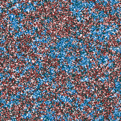
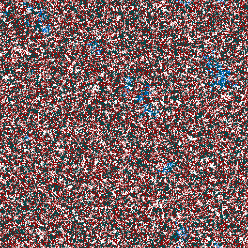
Figure 1: Snapshots of the spatial particle distribution for a single Monte Carlo simulation run of a stochastic predator-predator-prey Lotka–Volterra model on a $512\times 512$ square lattice with periodic boundary conditions at (from left to right) $t=0$ Monte Carlo Steps (MCS), $t=10\,000$ MCS, and $t=50\,000$ MCS, with predation rates $\lambda_{A}=0.5$, $\lambda_{B}=0.5$, predator death rates $\mu_{A}=0.126$, $\mu_{B}=0.125$, and prey reproduction rate $\sigma=1.0$. Only at most one particle per lattice site is allowed. Predator particles $A$ are indicated in blue, predators $B$ in red, and prey $C$ in dark green, while empty sites are shown in white.

In the stochastic lattice simulations, population densities are defined as the particle numbers for each species divided by the total number of lattice sites ($512\times 512$). We prepare the system so that the starting population densities of all three species are the same, here set to $0.3$ (particles/lattice site), and the particles are initially randomly distributed on the lattice. The system begins to leave this initial state as soon as the reactions start and the ultimate stationary state is only determined by the reaction rates, independent of the system’s initialization. We can test the simulation program by setting the parameters as $\lambda_{A}=\lambda_{B}=0.5$ and $\mu_{A}=\mu_{B}=0.125$. Since species $A$ and $B$ are now exactly the same, they coexist with an equal population density in the final stable state, as indeed observed in the simulations. We increase the value of $\mu_{A}$ by $0.001$ so that predator species $A$ is more likely to die than $B$. Fig. 1 shows the spatial distribution of the particles at $0$, $10\,000$, and $50\,000$ Monte Carlo Steps (MCS, from left to right), indicating sites occupied by $A$ particles in blue, $B$ in red, $C$ in green, and empty sites in white. As a consequence of the reaction scheme (1), specifically the clonal offspring production, surviving particles in effect remain close to other individuals of the same species and thus form clusters. After initiating the simulation runs, one typically observes these clusters to emerge quite quickly; as shown in Fig. 1, due to the tiny difference between the death rates $\mu_{A}-\mu_{B}>0$, the ‘weaker’ predator species $A$ gradually decreases its population number and ultimately goes extinct. Similar behavior is commonly observed also with other sets of parameters: For populations with equal predation rates, only the predator species endowed with a lower spontaneous death rate will survive. Fig. 2(a) records the temporal evolution of the three species’ population densities. After about $60\,000$ MCS, predator species $A$ has reached extinction, while the other two populations eventually approach non-zero constant densities. With larger values of $\mu_{A}$ such as $0.127$ or $0.13$, species $A$ dies out within a shorter time interval; the extinction time increases with diminishing death rate difference $|\mu_{A}-\mu_{B}|$.

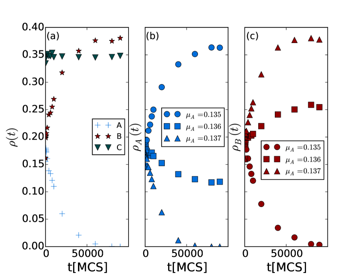
Figure 2: The two predator species cannot coexist in Monte Carlo simulations of the two-predator-one-prey model with fixed reaction rates. (a) Time evolution of the population densities with fixed reaction rates: predation rates $\lambda_{A}=0.5$, $\lambda_{B}=0.5$, predator death rates $\mu_{A}=0.126$, $\mu_{B}=0.125$, and prey reproduction rate $\sigma=1.0$; (b,c) temporal evolution of the population densities $\rho_{A}(t)$ and $\rho_{B}(t)$ with fixed $\lambda_{A}=0.55$, $\lambda_{B}=0.5$, $\mu_{B}=0.125$, and $\mu_{A}$ varying from $0.135$, $0.136$, to $0.137$. The curves in (b) and (c) sharing the same markers are from the same (single) simulation runs.

In Figs. 2(b) and (c), we set $\lambda_{A}=0.55$, $\lambda_{B}=0.5$, $\mu_{B}=0.125$, and various values of $\mu_{A}>0.13$. The larger rate $\lambda_{A}$ gives species $A$ an advantage over $B$ in the predation process, while the bigger rate $\mu_{A}$ enhances the likelihood of death for $A$ as compared to $B$. Upon increasing $\mu_{A}$ from $0.135$ to $0.137$, we observe a phase transition from species $B$ dying out to $A$ going extinct in this situation with competing predation and survival advantages. When $\mu_{A}$ thus exceeds a certain critical value (in this example near $0.136$), the disadvantages of high death rates cannot balance the gains due to a more favorable predation efficiency; hence predator species $A$ goes extinct. In general, whenever the reaction rates for predator species $A$ and $B$ are not exactly the same, either $A$ or $B$ will ultimately die out, while the other species remains in the system, coexisting with the prey $C$. This corresponds to actual biological systems where two kinds of animals share terrain and compete for the same food. Since there is no character displacement occurring between generations, the weaker species’ population will gradually decrease. This trend cannot be turned around unless the organisms improve their capabilities or acquire new skills to gain access to other food sources; either change tends to be accompanied by character displacements [32, 33, 34, 35].

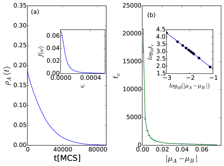
Figure 3: Characteristic decay time of the weaker predator species measured in Monte Carlo simulations of the two-predator-one-prey model with fixed reaction rates. (a) Main panel: temporal evolution of the predator population density $\rho_{A}(t)$ with predation rates $\lambda_{A}=0.5$, $\lambda_{B}=0.5$, predator death rates $\mu_{A}=0.126$, $\mu_{B}=0.125$, and prey reproduction rate $\sigma=1.0$. Inset: Fourier transform amplitude $f(\omega)$ of the predator density time series $\rho_{A}(t)$. (b) Main panel: characteristic decay time $t_{c}$ as obtained from the peak width of $f(\omega)$, versus the death rate difference $|\mu_{A}-\mu_{B}|$, with all other reaction rates fixed as in (a). Inset: the black dots show the data points $\log_{10}t_{c}$ versus $\log_{10}(|\mu_{A}-\mu_{B}|)$, while the blue straight line with slope $-1.23\pm 0.01$ is inferred from linear regression.

In order to quantitatively investigate the characteristic time for the weaker predator species to vanish, we now analyze the relation between the relaxation time $t_{c}$ of the weaker predator species ($A$ here) and the difference of death rates $|\mu_{A}-\mu_{B}|$ under the condition that $\lambda_{A}=\lambda_{B}$. Fig. 2(a) indicates that prey density (green triangles) reaches its stationary value much faster than the predator populations. When $|\mu_{A}-\mu_{B}|$ becomes close to zero, the system returns to a two-species model, wherein the relaxation time of the prey species $C$ is finite. However, the relaxation time of either predator species would diverge because it takes longer for the stronger species to remove the weaker one when they become very similar in their death probabilities. Upon rewriting eqs. (2) for $\lambda_{A}=\lambda_{B}$ by replacing the prey density $c(t)$ with its stationary value $\mu_{B}/\lambda_{B}$, we obtain a linearized equation for the weaker predator density: $\frac{da(t)}{dt}=-|\mu_{A}-\mu_{B}|a(t)$, describing exponential relaxation with decay time $t_{c}=1/|\mu_{A}-\mu_{B}|$.

We further explore the relation between the decay rate of the weak species population density and the reaction rates through Monte Carlo simulations. Fig. 3(a) shows an example of the weaker predator $A$ population density decay for fixed reaction rates $\lambda_{A}=0.5$, $\lambda_{B}=0.5$, $\mu_{A}=0.126$, $\mu_{B}=0.125$, and $\sigma=1.0$, and in the inset also the corresponding Fourier amplitude $f(\omega)=|\int e^{-i\omega t}\,\rho_{A}(t)\,dt|$ that is calculated by means of the fast Fourier transform algorithm. Assuming an exponential decay of the population density according to $\rho_{A}(t)\sim e^{-t/t_{c}}$, we identify the peak half-width at half maximum with the inverse relaxation time $1/t_{c}$. For other values of $\mu_{A}>0.125$, the measured relaxation times $t_{c}$ for the predator species $A$ are plotted in Fig. 3(b). We also ran simulations for various parameter values $\mu_{A}<0.125$, for which the predator population $B$ would decrease toward extinction instead of $A$, and measured the corresponding relaxation time for $\rho_{B}(t)$, plotted in Fig. 3(b) as well. The two curves overlap in the main panel of Fig. 3(b), confirming that $t_{c}$ is indeed a function of $|\mu_{A}-\mu_{B}|$ only. The inset of Fig. 3(b) demonstrates a power law relationship $t_{c}\sim|\mu_{A}-\mu_{B}|^{-z\nu}$ between the relaxation time and the reaction rate difference, with exponent $z\nu\approx-1.23\pm 0.01$ as inferred from the slope in the double-logarithmic graph via simple linear regression. This value is to be compared with the corresponding exponent $z\nu\approx 1.295\pm 0.006$ for the directed percolation (DP) universality class [36]. Directed percolation [38] represents a class of models that share identical values of their critical exponents at their phase transition points, and is expected to generically govern the critical properties at non-equilibrium phase transitions that separate active from inactive, absorbing states [39, 40]. Our result indicates that the critical properties of the two-predator-one-prey model with fixed reaction rates at the extinction threshold of one predator species appear to also be described by the DP universality class.

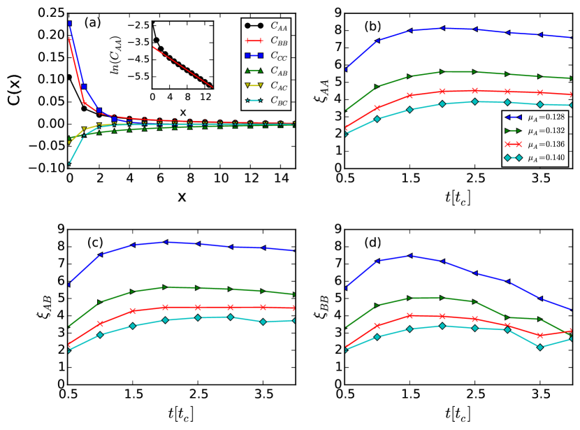
Figure 4: Time evolution for correlation lengths during Monte Carlo simulations of the two-predator-one-prey model with fixed reaction rates. (a) Main panel: correlation functions $C(x)$ after the system has evolved for one half of the relaxation time $0.5t_{c}\approx 2386$ MCS, with reaction rates $\lambda_{A}=0.5$, $\lambda_{B}=0.5$, $\mu_{A}=0.128$, $\mu_{B}=0.125$, and $\sigma=1.0$. Inset: $\ln(C_{AA})$ with a simple linear regression of the data points with $x\in[4,14]$ (red straight line) that yields the characteristic correlation decay length $\xi_{AA}\approx 5.8$. (b,c,d) Measured correlation lengths $\xi_{AA}$, $\xi_{AB}$, and $\xi_{BB}$ as function of the system evolution time t relative to $t_{c}$, with reaction rates as in (a) except (top to bottom) $\mu_{A}=0.128$ (blue left triangles), $0.132$ (green right triangles), $0.136$ (red crosses), and $0.140$ (cyan diamonds).

As already shown in Fig. 1, individuals from each species form clusters in the process of the stochastically occurring reactions (2). The correlation lengths $\xi$, obtained from equal-time correlation functions $C(x)$, characterize the average sizes of these clusters. The definition of the correlation functions between the different species $\alpha,\beta=A,B,C$ is $C_{\alpha\beta}(x)=\langle n_{\alpha}(x)n_{\beta}(0)\rangle-\langle n_{\alpha}(x)\rangle\langle n_{\beta}(0)\rangle$, where $n_{\alpha}(x)=0,1$ denotes the local occupation number of species $\alpha$ at site $x$. First choosing a lattice site, and then a second site at distance $x$ away, we note that the product $n_{\alpha}(x)n_{\beta}(0)=1$ only if a particle of species $\beta$ is located on the first site, and a particle of species $\alpha$ on the second site; otherwise the product equals $0$. We then average over all sites to obtain $\langle n_{\alpha}(x)n_{\beta}(0)\rangle$. $\langle n_{\alpha}(x)\rangle$ represents the average population density of species $\alpha$.

In our Monte Carlo simulations we find that although the system has not yet reached stationarity at $0.5\,t_{c}$, its correlation functions do not vary appreciably during the subsequent time evolution. This is demonstrated in Figs. 4(b-d) which show the measured correlation lengths from $0.5\,t_{c}$ to $3.75\,t_{c}$, during which time interval the system approaches its quasi-stationary state. The main panel in Fig. 4(a) shows the measured correlation functions after the system has evolved for $0.5\,t_{c}\approx 2386$ MCS, with predator $A$ death rate $\mu_{A}=0.128$. Individuals from the same species are evidently spatially correlated, as indicated by the positive values of $C_{\alpha\alpha}$. Particles from different species, on the other hand, display anti-correlations. The inset demonstrates exponential decay: $C_{AA}(x)\sim e^{-|x|/\xi_{AA}}$, where $\xi_{AA}$ is obtained from linear regression of $ln(C_{AA}(x))$. In the same manner, we calculate the correlation length $\xi_{AA}$, $\xi_{BB}$, and $\xi_{AB}$ for every $0.5\,t_{c}$ the system evolves, for different species $A$ death rates $\mu_{A}=0.128$, $0.132$, $0.136$, and $0.140$, respectively. Fig. 4(b) shows that predator $A$ clusters increase in size by about two lattice constants within $1.5\,t_{c}$ after the reactions begin, and then stay almost constant. In the meantime, the total population number of species $A$ decreases exponentially as displayed in Fig. 3, which indicates that the number of predator $A$ clusters decreases quite fast. Fig. 4(c) does not show prominent changes for the values of $\xi_{AB}(t)$ as the reaction time $t$ increases, demonstrating that species $A$ and $B$ maintain a roughly constant distance throughout the simulation. In contrast, Fig. 4(d) depicts a significant temporal evolution of $\xi_{BB}(t)$: the values of $\xi_{BB}$ are initially close to those of $\xi_{AA}$, because of the coevolution of both predator species $A$ and $B$; after several decay times $t_{c}$, however, there are few predator $A$ particles left in the system. The four curves for $\xi_{BB}$ would asymptotically converge after species $A$ has gone fully extinct.

To summarize this section, the two indirectly competing predator species cannot coexist in the lattice three-species model with fixed reaction rates. The characteristic time for the weaker predator species to go extinct diverges as its reaction rates approach those of the stronger species. We do not observe large fluctuations of the correlation lengths during the system’s time evolution, indicating that spatial structures remain quite stable throughout the Monte Carlo simulation.

3 Introducing character displacement

3.1 Model description

The Lotka–Volterra model simply treats the individuals in each population as particles endowed with uniform birth, death, and predation rates. This does not reflect a natural environment where organisms from the same species may still vary in predation efficiency and death or reproduction rates because of their size, strength, age, affliction with disease, etc. In order to describe individually varying efficacies, we introduce a new character $\eta\in[0,1]$, which plays the role of an effective trait that encapsulates the effects of phenotypic changes and behavior on the predation / evasion capabilities, assigned to each individual particle [31]. When a predator $A_{i}$ (or $B_{j}$) and a prey $C_{k}$ occupy neighboring lattice sites, we set the probability $(\eta_{Ai}+\eta_{Ck})/2$ [or $(\eta_{Bj}+\eta_{Ck})/2$] for $C_{k}$ to be replaced by an offspring predator $A_{z}$ (or $B_{z}$). The indices $i$, $j$, $k$, and $z$ here indicate specific particles from the predator populations $A$ or $B$, the prey population $C$, and the newly created predator offspring in either the $A$ or $B$ population, respectively. In order to confine all reaction probabilities in the range $[0,1]$, the efficiency $\eta_{Az}$ (or $\eta_{Bz}$) of this new particle is generated from a truncated Gaussian distribution that is centered at its parent particle efficiency $\eta_{Ai}$ (or $\eta_{Bj}$) and restricted to the interval $[0,1]$, with a certain prescribed distribution width (standard deviation) $\omega_{\eta A}$ (or $\omega_{\eta B}$). When a parent prey individual $C_{i}$ gives birth to a new offspring particle $C_{z}$, the efficiency $\eta_{Cz}$ is generated through a similar scheme with a given width $\omega_{\eta C}$. Thus any offspring’s efficiency entails inheriting its parent’s efficacy but with some random mutational adaptation or differentiation. The distribution width $\omega$ models the potential range of the evolutionary trait change: for larger $\omega$, an offspring’s efficiency is more likely to differ from its parent particle. Note that the width parameters $\omega$ here are unique for particles from the same species, but may certainly vary between different species. In previous work, we studied a two-species system (one predator and one prey) with such demographic variability [31, 37]. In that case, the system arrived at a final steady state with stable stationary positive species abundances. On a much faster time scale than the species density relaxation, their respective efficiency $\eta$ distributions optimized in this evolutionary dynamics, namely: the predators’ efficacies rather quickly settled at a distribution centered at values near $1$, while the prey efficiencies tended to small values close to $0$. This represents a coevolution process wherein the predator population on average gains skill in predation, while simultaneously the prey become more efficient in evasion so as to avoid being killed.

3.2 Quasi-species mean-field equations and numerical solution

We aim to construct a mean-field description in terms of quasi-subspecies that are characterized by their predation efficacies $\eta$. To this end, we discretize the continuous interval of possible efficiencies $0\leq\eta\leq 1$ into $N$ bins, with the bin midpoint values $\eta_{i}=(i+1/2)/N$, $i=0,\ldots,N-1$. We then consider a predator (or prey) particle with an efficacy value in the range $\eta_{i}-1/2\leq\eta\leq\eta_{i}+1/2$ to belong to the predator (or prey) subspecies $i$. The probability that an individual of species $A$ with predation efficiency $\eta_{1}$ produces offspring with efficiency $\eta_{2}$ is assigned by means of a reproduction probability function $f(\eta_{1},\eta_{2})$. In the binned version, we may use the discretized form $f_{ij}=f(\eta_{i},\eta_{j})$. Similarly, we have a reproduction probability function $g_{ij}$ for predator species $B$ and $h_{ij}$ for the prey $C$. Finally, we assign the arithmetic mean $\lambda_{ik}=(\eta_{i}+\eta_{k})/2$ to set the effective predation interaction rate of predator $i$ with prey $k$ [31, 37].

These prescriptions allow us to construct the following coupled mean-field rate equations for the temporal evolution of the subspecies populations:

$$\begin{split}\frac{\partial a_{i}(t)}{\partial t}&=-\mu a_{i}(t)+\sum_{jk}\lambda_{kj}f_{ki}a_{k}(t)c_{j}(t)\,,\\ \frac{\partial b_{i}(t)}{\partial t}&=-\mu b_{i}(t)+\sum_{jk}\lambda_{kj}g_{ki}b_{k}(t)c_{j}(t)\,,\\ \frac{\partial c_{i}(t)}{\partial t}&=\sigma\sum_{k}h_{ki}c_{k}(t)\bigg{(}1-\frac{\sum_{z}[a_{z}(t)+b_{z}(t)+c_{z}(t)]}{K}\bigg{)}\\ &\quad-\sum_{j}\lambda_{ji}a_{j}(t)c_{i}(t)-\sum_{j}\lambda_{ji}b_{j}(t)c_{i}(t)\,.\end{split}$$ (3)

Steady-state solutions are determined by setting the time derivatives to zero, $\partial a_{i}(t)/\partial t=\partial b_{i}(t)/\partial t=\partial c_{i}(t)/\partial t=0$. Therefore, the steady-state particle counts can always be found by numerically solving the coupled implicit equations

$$\begin{split}\mu a_{i}&=\sum_{jk}\lambda_{kj}f_{ki}a_{k}c_{j}\,,\\ \mu b_{i}&=\sum_{jk}\lambda_{kj}g_{ki}b_{k}c_{j}\,,\\ \sigma\sum_{k}h_{ki}c_{k}(t)\bigg{(}1-\frac{\sum_{z}[a_{z}(t)+b_{z}(t)+c_{z}(t)]}{K}\bigg{)}&=\sum_{j}\lambda_{ji}a_{j}c_{i}+\sum_{j}\lambda_{ji}b_{j}c_{i}\,.\end{split}$$ (4)

In the special case of a uniform inheritance distribution for all three species, $f_{ij}=g_{ij}=h_{ij}=1/N$, the above equations can be rewritten as

$$\begin{split}\mu(a_{i}+b_{i})&=\frac{1}{N}\sum_{jk}\lambda_{kj}(a_{k}+b_{k})c_{j}\,,\\ \frac{1}{N}\sigma\sum_{k}c_{k}\bigg{(}1-\frac{\sum_{z}[a_{z}(t)+b_{z}(t)+c_{z}(t)]}{K}\bigg{)}&=\sum_{j}\lambda_{ji}(a_{j}+b_{j})c_{i}\,,\end{split}$$ (5)

whose non-zero solutions are

$$\begin{split}&(i)\quad a_{i}=0,\quad\frac{b_{i}}{\sum_{j}b_{j}}=\frac{1}{N}\,,\quad\frac{c_{i}}{\sum_{j}c_{j}}=\frac{2}{N\ln 3}\frac{1}{1+2\eta_{i}}\,;\\ &(ii)\quad b_{i}=0,\quad\frac{a_{i}}{\sum_{j}a_{j}}=\frac{1}{N}\,,\quad\frac{c_{i}}{\sum_{j}c_{j}}=\frac{2}{N\ln 3}\frac{1}{1+2\eta_{i}}\,;\\ &(iii)\quad\frac{a_{i}+b_{i}}{\sum_{j}(a_{j}+b_{j})}=\frac{1}{N}\,,\quad\frac{c_{i}}{\sum_{j}c_{j}}=\frac{2}{N\ln 3}\frac{1}{1+2\eta_{i}}\,.\end{split}$$ (6)

We could not obtain the full time-dependent solutions to the mean-field equations in closed form. We therefore employed an explicit fourth-order Runge–Kutta scheme to numerically solve eqs. (3), using a time step of $\Delta t=0.1$, the initial condition $a_{i}(t=0)=b_{i}(t=0)=c_{i}(t=0)=1/(3N)$ for $i=1,...,N$, a number of subspecies $N=100$, and the carrying capacity $K=1$. An example for the resulting time evolution of the predator $B$ density is shown in Fig. 5(b); its caption provides the remaining parameter values.

3.3 Lattice simulation

We now proceed to Monte Carlo simulations for this system on a two-dimensional square lattice, and first study the case where trait evolution is solely introduced to the predation efficiencies $\eta$. In these simulation, the values of $\mu$ and $\sigma$ are held fixed, as is the nonzero distribution width $\omega$, so that an offspring’s efficiency usually differs from its parent particle. In accord with the numerical solutions for the mean-field equations (3), we find that the three-species system (predators $A$ and $B$, prey $C$) is generically unstable and will evolve into a final two-species steady state, where one of the predator species goes extinct, depending only on the value of $\omega$ (given that $\mu$ and $\sigma$ are fixed).

At the beginning of the simulation runs, the initial population densities, which are the particle numbers of each species divided by the lattice site number, are assigned the same value $0.3$ for all the three species. The particles are randomly distributed on the lattice sites. We have checked that the initial conditions do not influence the final state by varying the initial population densities and efficiencies. We fix the predator death rate to $\mu=0.125$ for both species $A$ and $B$, and set the prey reproduction rate as $\sigma=1.0$. The predation efficacies for all particles are initialized at $\eta=0.5$. We have varied the values of the distribution width $\omega$ and observed the final (quasi-)steady states. For the purpose of simplification, we fix $\omega_{\eta A}=\omega_{\sigma C}=0.1$, and compare the final states when various values of $\omega_{\eta B}$ are assigned.

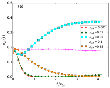
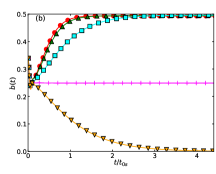
Figure 5: (a) Stochastic lattice simulation of the two-predator-one-prey model with ‘Darwinian’ evolution introduced only for the predation efficiency $\eta$: predator population density $\rho_{B}(t)$ for various values of the predation efficiency distribution width $\omega_{\eta B}=0.001$ (red dots), $0.01$ (green triangles up), $0.05$ (blue squares), $0.1$ (pink crosses), and $0.15$ (orange triangles down), with all other reaction rates held fixed at $\mu=0.125$, $\sigma=1.0$, and $\omega_{\eta A}=\omega_{\eta C}=0.1$; Monte Carlo time $t$ rescaled with the relaxation time $t_{0s}=1900$ MCS of the curve for $\omega_{\eta B}=0.05$. (b) Numerical solution of the mean-field eqs. (3) with $b(t)=\frac{1}{N}\sum_{i}b_{i}(t)$ denoting the average subspecies density. The parameters are set at the same values as for the lattice simulations; time $t$ is again normalized with the relaxation time $t_{0}=204.32$ of the curve for $\omega_{\eta B}=0.05$ curve to allow direct comparison with the simulation data. Note that the limited carrying capacity in both lattice simulations and the mean-field model introduces strong damping which suppresses the characteristic LV oscillations.

Fig. 5(a) shows the population density $\rho_{B}(t)$ of predator species $B$ with the listed values for $\omega_{\eta B}$. Each curve depicts a single simulation run. When $\omega_{\eta B}>0.1$, the $\rho_{B}(t)$ quickly tends to zero; following the extinction of the $B$ species, the system reduces to a stable $A$-$C$ two-species predator-prey ecology. When $\omega_{\eta B}=0.1$, there is no difference between species $A$ and $B$, so both populations survive with identical final population density; for $\omega_{\eta B}=0.01,0.05$, predator species $A$ finally dies out and the system is reduced to a $B$-$C$ two-species system; we remark that the curve for $\omega_{\eta B}=0.01$ (green triangles up) decreases first and then increases again at very late time points which is only partially shown in the graph. For $\omega_{\eta B}=0.001$ and even smaller, $\rho_{B}(t)$ goes to zero quickly, ultimately leaving an $A$-$C$ two-species system. We tried another $100$ independent runs and obtained the same results: for $\omega_{\eta B}\neq\omega_{\eta A}$, one of the predator species will vanish and the remaining one coexists with the prey $C$. When $\omega_{\eta B}$ is smaller than $\omega_{\eta A}$ but not too close to zero, predator species $B$ prevails, while $A$ goes extinct. For $\omega_{\eta B}=0$, there is of course no evolution for these predators at all, thus species $A$ will eventually outlast $B$. Thus there exists a critical value $\omega_{Bc}$ for the predation efficacy distribution width $\omega_{\eta B}$, at which the probability of either predator species $A$ or $B$ to win the ‘survival game’ is $50\%$. When $\omega_{Bc}<\omega_{\eta B}<\omega_{\eta A}$, $B$ has an advantage over $A$, i.e., the survival probability of $B$ is larger than $50\%$; conversely, for $\omega_{Bc}>\omega_{\eta B}$, species $A$ outcompetes $B$. This means that the evolutionary ‘speed’ is important in a finite system, and is determined by the species plasticity $\omega$.

Fig. 5(b) shows the numerical solution of the associated mean-field model defined by eqs. (3). In contrast to the lattice simulations, small $\omega_{\eta B}$ do not yield extinction of species $B$; this supports the notion that the reentrant phase transition from $B$ to $A$ survival at very small values of $\omega_{\eta B}$ is probably a finite-size effect, as discussed below. Because of the non-zero carrying capacity, oscillations of population densities are largely suppressed in both Monte Carlo simulations and the mean-field model. Spatio-temporal correlations in the stochastic lattice system rescale the reaction rates, and induce a slight difference between the steady-state population densities in Figs. 5(a) and (b) even though the microscopic rate parameters are set to identical values. For example, for $\omega_{\eta B}=0.1$, the quasi-stationary population density of predator species $B$ is $\approx 0.19$ (pink plus symbols) in the lattice model, but reaches $0.25$ in the numerical solution of the mean-field rate equations. Time $t$ is measured in units of Monte Carlo Steps (MCS) in the simulation; there is no method to directly convert this (discrete) Monte Carlo time to the continuous time in the mean-field model. For the purpose of comparing the decay of population densities, we therefore normalize time $t$ by the associated relaxation times $t_{0s}=1900$ MCS in the simulations and $t_{0}=204.32$ in the numerical mean-field solution; both are calculated by performing a Fourier transform of the time-dependent prey densities $\rho_{B}(t)$ and $b(t)$ for $\omega_{\eta B}=0.05$ (blue squares).

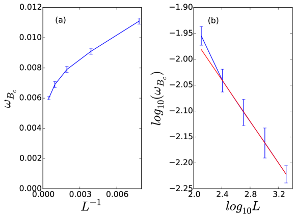
Figure 6: (a) Stochastic lattice simulation of the two-predator-one-prey model with ‘Darwinian’ evolution only introduced to the predation efficiencies $\eta$: critical distribution width $\omega_{Bc}$ as a function of the inverse linear system size $1/L$, with predator death rate $\mu=0.125$, prey reproduction rate $\sigma=1.0$, and $\omega_{\eta A}=0.1$. The data are obtained for linear system sizes $L\in[128,256,512,1024,2048]$. (b) Double-logarithmic plot of the critical width $\omega_{Bc}$ as a function of system size $L$; the red straight line represents a simple linear regression of the four points with $L\in[256,512,1024,2048]$, with slope $-0.2$. The point with $L=128$ presumably deviates from this straight line due to additional strong finite-size effects.

Our method to estimate $\omega_{Bc}$ was to scan the value space of $\omega_{\eta B}\in[0,1]$, and perform $1000$ independent simulation runs for each value until we found the location in this interval where the survival probability for either $A$ or $B$ predator species was $50\%$. With the simulations on a $512\times 512$ system and all the parameters set as mentioned above, $\omega_{Bc}$ was measured to be close to $0.008$. We repeated these measurements for various linear system sizes $L$ in the range $[128,2048]$. Fig. 6(a) shows $\omega_{Bc}$ as a function of $1/L$, indicating that $\omega_{Bc}$ decreases with a divergent rate as the system is enlarged. Because of limited computational resources, we were unable to extend these results to even larger systems. According to the double-logarithmic analysis shown in Fig. 6(b), we presume that $\omega_{Bc}$ would fit a power law $\omega_{Bc}\sim L^{-\theta}$ with exponent $\theta=0.2$. This analysis suggests that $\omega_{Bc}=0$ in an infinitely large system, and that the reentrant transition from $B$ survival to $A$ survival in the range $\omega_{\eta B}\in[0,\omega_{\eta A}]$ is likely a finite-size effect. We furthermore conclude that in the three-species system (two predators and a single prey) the predator species with a smaller value of the efficiency distribution width $\omega$ always outlives the other one. A smaller $\omega$ means that the offspring’s efficiency is more centralized at its parent’s efficacy; mutations and adaptations have smaller effects. Evolution may thus optimize the overall population efficiency to higher values and render this predator species stronger than the other one with larger $\omega$, which is subject to more, probably deleterious, mutations. These results were all obtained from the measurements with $\omega_{\eta A}=0.1$. However, other values of $\omega_{\eta A}$ including $0.2$, $0.3$, and $0.4$ were tested as well, and similar results observed.

Our numerical observation that two predator species cannot coexist contradicts observations in real ecological systems. This raises the challenge to explain multi-predator-species coexistence. Notice that ‘Darwinian’ evolution was only applied to the predation efficiency in our model. However, natural selection could also cause lower predator death rates and increased prey reproduction rates so that their survival chances would be enhanced in the natural selection competition. One ecological example are island lizards that benefit from decreased body size because large individuals will attract attacks from their competitors [5]. In the following, we adjust our model so that the other two reaction rates $\mu$ and $\sigma$ do not stay fixed anymore, but instead evolve by following the same mechanism as previously implemented for the predation efficacies $\eta$. The death rate of an offspring predator particle is hence generated from a truncated Gaussian distribution centered at its parent’s value, with positive standard deviations $\omega_{\mu A}$ and $\omega_{\mu B}$ for species $A$ and $B$, respectively. The (truncated) Gaussian distribution width for the prey reproduction rate is likewise set to a non-zero value $\omega_{\sigma}$.

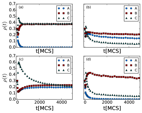
Figure 7: Population densities $\rho(t)$ from Monte Carlo simulations with ‘Darwinian’ evolution introduced to both the predation efficiencies $\eta$ and predator death rates $\mu$, while the prey reproduction rate stays fixed at $\sigma=1.0$. The species are indicated as blue dots for $A$, red squares for $B$, and green triangles for $C$. The final states are in (a) $A$ extinction; (b) and (c) transient three-species coexistence; and (d) $B$ extinction, with $\omega_{\eta A}=0.11$, $\omega_{\mu A}=0.3$, $\omega_{\mu B}=0.125$ in (a), $\omega_{\eta A}=0.08$, $\omega_{\mu A}=0.1$, $\omega_{\mu B}=0.09$ in (b), $\omega_{\eta A}=0.08$, $\omega_{\mu A}=0.4$, $\omega_{\mu B}=0.39$ in (c), and $\omega_{\eta A}=0.08$, $\omega_{\mu A}=0.4$, $\omega_{\mu B}=0.09$ in (d), while $\omega_{\eta B}=0.1$, $\omega_{\eta C}=0.1$, $\omega_{\sigma C}=0$ for all four plots.

In the simulations, the initial population densities for all three species are set at $0.3$ with the particles randomly distributed on the lattice. The reaction rates and efficiencies for these first-generation individuals were chosen as $\eta_{A0}=\eta_{B0}=\eta_{C0}=0.5$, $\mu_{A0}=\mu_{B0}=0.125$, and $\sigma_{0}=1.0$. With this same initial set, we ran simulations with different values of the Gaussian distribution widths $\omega$. Figure 7 displays the temporal evolution of the three species’ population densities with four sets of given widths $\omega$: In Fig. 7(a), $\omega_{\eta A}=0.11$, $\omega_{\eta B}=0.1$, $\omega_{\eta C}=0.1$, $\omega_{\mu A}=0.3$, $\omega_{\mu B}=0.125$, and $\omega_{\sigma C}=0$. Since a smaller width $\omega$ gives advantages to the corresponding species, $\omega_{\eta B}<\omega_{\eta A}$ and $\omega_{\mu B}<\omega_{\mu A}$ render predators $B$ stronger than $A$ in general. As the graph shows, species $A$ dies out quickly and finally only $B$ and $C$ remain in the system. In all four cases, the prey $C$ stay active and do not become extinct.

However, it is not common that a species is stronger than others in every aspect, so we next set $\omega$ so that $A$ has advantages over $B$ in predation, i.e., $\omega_{\eta A}<\omega_{\eta B}$, but is disadvantaged through broader-distributed death rates $\omega_{\mu A}>\omega_{\mu B}$. In Fig. 7(b), $\omega_{\eta A}=0.08$, $\omega_{\eta B}=0.1$, $\omega_{\eta C}=0.1$, $\omega_{\mu A}=0.1$, $\omega_{\mu B}=0.09$, and $\omega_{\sigma C}=0$; in Fig. 7(c), $\omega_{\eta A}=0.08$, $\omega_{\eta B}=0.1$, $\omega_{\eta C}=0.1$, $\omega_{\mu A}=0.4$, $\omega_{\mu B}=0.39$, and $\omega_{\sigma C}=0$. In either case, none of the three species becomes extinct after $10\,000$ MCS, and three-species coexistence will persist at least for much longer time. Monitoring the system’s activity, we see that the system remains in a dynamic state with a large amount of reactions happening. When we repeat the measurements with other independent runs, similar results are observed, and we find the slow decay of the population densities to be rather insensitive to the specific values of the widths $\omega$. As long as we implement a smaller width $\omega$ for the $A$ predation efficiency than for the $B$ species, but a larger one for its death rates, or vice versa, three-species coexistence emerges. Of course, when the values of the standard deviations $\omega$ differ too much between the two predator species, one of them may still approach extinction fast. One example is shown in Fig. 7(d), where $\omega_{\eta A}=0.08$, $\omega_{\eta B}=0.1$, $\omega_{\eta C}=0.1$, $\omega_{\mu A}=0.4$, $\omega_{\mu B}=0.09$, and $\omega_{\sigma C}=0$; since $\omega_{\mu A}$ is about five times larger than $\omega_{\mu B}$ here, the predation advantage of species $A$ cannot balance its death rate disadvantage, and consequently species $A$ is driven to extinction quickly. Yet the coexistence of all three competing species in Figs. 7(b) and (c) does not persist forever, and at least one species will die out eventually, after an extremely long time. Within an intermediate time period, which still amounts to thousands of generations, they can be regarded as quasi-stable because the decay is very slow. This may support the idea that in real ecosystems perhaps no truly stable multiple-species coexistence exists, and instead the competing species are in fact under slow decay which is not noticeable within much shorter time intervals. In Figs. 7(a) and (d), the predator $A$ population densities decay exponentially with relaxation times of order $100$ MCS, while the corresponding curves in (b) and (c) approximately follow algebraic functions (power law decay).

However, we note that in the above model implementation the range of predator death rates $\mu$ was the entire interval $[0,1]$, which gives some individuals a very low chance to decay. Hence these particles will stay in the system for a long time, which accounts for the long-lived transient two-predator coexistence regime. To verify this assumption, we set a positive lower bound on the predators’ death rates, preventing the presence of near-immortal individuals. We chose the value of the lower bound to be $0.001$, with the death rates $\mu$ for either predator species generated in the predation and reproduction processes having to exceed this value. Indeed, we observed no stable three-species coexistence state, i.e., one of the predator species was invariably driven to extinction, independent of the values of the widths $\omega$, provided they were not exactly the same for the two predator species. To conclude, upon introducing a lower bound for their death rates, the two predator species cannot coexist despite their dynamical evolutionary optimization.

4 Effects of direct competition between both predator species

4.1 Inclusion of direct predator competition and mean-field analysis

We proceed to include explicit direct competition between both predator species in our model. The efficiencies of predator particles are most likely to be different since they are randomly generated from truncated Gaussian distributions. When a strong $A$ individual (i.e., with a large predation efficacy $\eta$) meets a weaker $B$ particle on an adjacent lattice site, or vice versa, we now allow predation between both predators to occur. Direct competition is common within predator species in nature. For example, a strong lizard may attack and even kill a small lizard to occupy its habitat. A lion may kill a wolf, but an adult wolf might kill an infant lion. Even though cannibalism occurs in nature as well, we here only consider direct competition and predation between different predator species. In our model, direct competition between the predator species is implemented as follows: For a pair of predators $A_{i}$ and $B_{j}$ located on neighboring lattice sites and endowed with respective predation efficiencies $\eta_{Ai}$ and $\eta_{Bj}<\eta_{Ai}$, particle $B_{j}$ is replaced by a new $A$ particle $A_{z}$ with probability $\eta_{Ai}-\eta_{Bj}$; conversely, if $\eta_{Ai}<\eta_{Bj}$, there is a probability $\eta_{Bj}-\eta_{Ai}$ that $A_{i}$ is replaced by a new particle $B_{z}$.

We first write down and analyze the mean-field rate equations for the simpler case when the predator species compete directly without evolution, i.e., all reaction rates are uniform and constant. We assume that $A$ is the stronger predator with $\lambda_{A}>\lambda_{B}$, hence only the reaction $A+B\to A+A$ is allowed to take place with rate $\lambda_{A}-\lambda_{B}$, but not its complement, supplementing the original reaction scheme listed in (1). The associated mean-field rate equations read

$$\begin{split}\frac{da(t)}{dt}&=-\mu_{A}a(t)+\lambda_{A}a(t)c(t)+(\lambda_{A}-\lambda_{B})a(t)b(t)\,,\\ \frac{db(t)}{dt}&=-\mu_{B}b(t)+\lambda_{B}b(t)c(t)-(\lambda_{A}-\lambda_{B})a(t)b(t)\,,\\ \frac{dc(t)}{dt}&=\sigma c(t)\bigg{[}1-\frac{a(t)+b(t)+c(t)}{K}\bigg{]}-\lambda_{A}a(t)c(t)-\lambda_{B}b(t)c(t)\,,\end{split}$$ (7)

with the non-zero stationary solutions

$$\begin{split}(i)\quad a=0\,,\quad b=\frac{\sigma(K\lambda_{B}-\mu_{B})}{\lambda_{B}(\sigma+K\lambda_{B})}\,,\quad c=\frac{\mu_{B}}{\lambda_{B}}\,,\\ (ii)\quad a=\frac{\sigma(K\lambda_{A}-\mu_{A})}{\lambda_{A}(\sigma+K\lambda_{A})}\,,\quad b=0\,,\quad c=\frac{\mu_{A}}{\lambda_{A}}\,,\\ (iii)\quad a+b+c=\frac{\mu_{A}-\mu_{B}}{\lambda_{A}-\lambda_{B}}\,,\quad\text{when}\quad a(0)+b(0)+c(0)=\frac{\mu_{A}-\mu_{B}}{\lambda_{A}-\lambda_{B}}\,.\end{split}$$ (8)

Within this mean-field theory, three-species coexistence states exist only when the total initial population density is set to $a(0)+b(0)+c(0)=\frac{\mu_{A}-\mu_{B}}{\lambda_{A}-\lambda_{B}}$. In our lattice simulations, however, we could not observe any three-species coexistence state even when we carefully tuned one reaction rate with all others held fixed.

Next we reinstate ‘Darwinian’ evolution for this extended model with direct competition between the predator species. We utilize the function $\hat{\lambda}_{ij}=|\eta_{i}-\eta_{j}|$ to define the reaction rate between predators $A$ and $B$. For the case that the predator death rate $\mu$ is fixed for both species $A$ and $B$, the ensuing quasi-subspecies mean-field equations are

$$\begin{split}\frac{\partial a_{i}(t)}{\partial t}&=-\mu a_{i}(t)+\sum_{jk}\lambda_{kj}f_{ki}a_{k}(t)c_{j}(t)+\sum_{j<k}\hat{\lambda}_{kj}f_{ki}a_{k}(t)b_{j}(t)\\ &\quad-\sum_{j>i}\hat{\lambda}_{ij}a_{i}(t)b_{j}(t)\,,\\ \frac{\partial b_{i}(t)}{\partial t}&=-\mu b_{i}(t)+\sum_{jk}\lambda_{kj}g_{ki}b_{k}(t)c_{j}(t)+\sum_{j<k}\hat{\lambda}_{kj}g_{ki}b_{k}(t)a_{j}(t)\\ &\quad-\sum_{j>i}\hat{\lambda}_{ji}b_{i}(t)a_{j}(t)\,\\ \frac{\partial c_{i}(t)}{\partial t}&=\sigma\sum_{j}h_{ji}c_{j}(t)\bigg{(}1-\frac{\sum_{z}[a_{z}(t)+b_{z}(t)+c_{z}(t)]}{K}\bigg{)}\\ &\quad-\sum_{j}\lambda_{ji}[a_{j}(t)+b_{j}(t)]c_{i}(t)\,.\end{split}$$ (9)

Since a closed set of solutions for eqs. (9) is very difficult to obtain, we resort to numerical integration. As before, we rely on an explicit fourth-order Runge–Kutta scheme with time step $\Delta t=0.1$, initial conditions $a_{i}(t=0)=b_{i}(t=0)=c_{i}(t=0)=1/N$, number of subspecies $N=100$, and carrying capacity $K=3$. Four examples for such numerical solutions of the quasi-subspecies mean-field equations are shown in Fig. 8, and will be discussed in the following subsection.

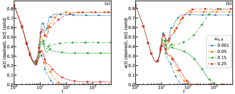
Figure 8: Numerical solutions of the mean-field equations (9) for the two-predator subspecies densities $a(t)=\frac{1}{N}\sum_{i}a_{i}(t)$ (dashed) and $b(t)=\frac{1}{N}\sum_{i}b_{i}(t)$ (solid) for different distribution widths $\omega_{\eta,B}$ and the parameters $\omega_{\eta,A}=0.14$, $\omega_{\eta,C}=\infty$, $\sigma=1$, and $\mu=0.5$. (a) Population densities in the presence of direct predator-predator competition; and (b) in the absence of this competition. Note that three-species coexistence is only possible when direct predator-predator competition is explicitly implemented.

4.2 The quasi-stable three-species coexistence region

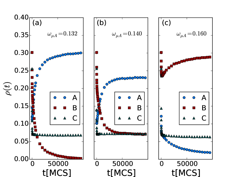
Figure 9: Data obtained from Monte Carlo simulations where both direct competition between both predator species as well as evolutionary dynamics are introduced: Temporal population density record with $\omega_{\eta A}=0.1$, $\omega_{\eta B}=0.15$, $\omega_{\mu B}=0.1$ and $\omega_{\mu A}=0.132$, $0.140$, $0.160$ (from left to right) with species $A$ indicated with blue dots, $B$ red-dashed, and $C$ with green triangles.

For the three-species system with two predators $A$, $B$ and prey $C$, we now introduce ‘Darwinian’ evolution to both the predator death rates $\mu$ and the predation efficiencies $\eta$. In addition, we implement direct competition between the predators $A$ and $B$. We set the lower bound of the death rates $\mu$ to $0.001$ for both predator species. The simulations are performed on a $512\times 512$ square lattice with periodic boundary conditions. Initially, individuals from all three species are randomly distributed in the system with equal densities $0.3$. Their initial efficiencies are chosen as $\eta_{A}=0.5=\eta_{B}$ and $\eta_{C}=0$. Since there is no evolution of the prey efficiency, $\eta_{C}$ will stay zero throughout the simulation. The distribution widths for the predation efficiencies are fixed to $\omega_{\eta A}=0.1$ and $\omega_{\eta B}=0.15$, giving species $A$ an advantage over $B$ in the non-linear predation process. We select the width of the death rate distribution of species $B$ as $\omega_{\mu B}=0.1$. If $\omega_{\mu A}$ is also chosen to be $0.1$, the $B$ population density would decay exponentially. $\omega_{\mu A}>\omega_{\mu B}=0.1$ is required to balance species $A$’s predation adaptation advantage so that stable coexistence is possible. Figure 9 shows the population densities resulting from our individual-based Monte Carlo simulations as a function of time, for different values $\omega_{\mu A}=0.132$, $0.140$, and $0.160$. These graphs indicate the existence of phase transitions from species $B$ extinction in Fig. 9(a) to predator $A$-$B$ coexistence in Fig. 9(b), and finally to $A$ extinction in Fig. 9(c)). In Fig. 9(a), species $A$ is on average more efficient than $B$ in predation, but has higher death rates. Predator species $B$ is in general the weaker one, and hence goes extinct after about $100\,000$ MCS. Figure 9(b) shows a (quasi-)stable coexistence state with neither predator species dying out within our simulation time. In Fig. 9(c), $\omega_{\mu A}$ is set so high that $A$ particles die much faster than $B$ individuals, so that finally species $A$ would vanish entirely.

Figure 8(a) displays the time evolution for the solutions of the corresponding quasi-subspecies mean-field model (9) for four different values of the species $B$ efficiency width $\omega_{\eta,B}$. In particular, it shows that there is a region of coexistence in which both predator species reach a finite steady-state density, supporting the Monte Carlo results from the stochastic lattice model. In contrast, numerical solutions of eqs. (9) with $\hat{\lambda}_{ij}=0$, equivalent to eqs. (3), exhibit no three-species coexistence region; see Fig. 8(b).

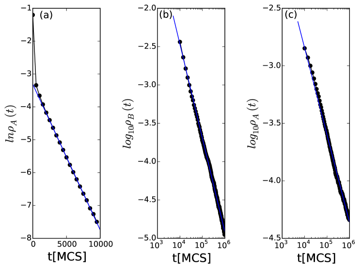
Figure 10: Monte Carlo simulations with direct predator competition: (a) Exponential decay of the predator population density $\rho_{A}(t)$ with $\omega_{\mu A}=0.2$, $\omega_{\eta A}=0.1$, $\omega_{\eta B}=0.15$, and $\omega_{\mu B}=0.1$; the blue straight line is obtained from a linear regression of the data points for $x\geq 2000$, with slope $-0.00044$. (b) Algebraic power-law decay of the predator $B$ species density with $\omega_{\mu A}=0.136$ and the other parameters set as in (a). (c) Power-law decay of $\rho_{A}(t)$ for $\omega_{\mu A}=0.159$. The black dots are measured population densities from the simulations, while the blue straight lines indicate simple linear regressions of the simulation data.

At an active-to-absorbing phase transition threshold, one should anticipate the standard critical dynamics phenomenology for a continuous phase transition: exponential relaxation with time becomes replaced by much slower algebraic decay of the population density [39, 40]. We determine the three-species coexistence range for our otherwise fixed parameter set to be in the range $\omega_{\mu A}\in[0.136,0.159]$. Figure 10(a) shows an exponential decay of the predator population $A$ density with $\omega_{\mu A}=0.2$, deep in the absorbing extinction phase. The system would attain $B$-$C$ two-species coexistence within of the order $10^{4}$ MCS. We also ran the Monte Carlo simulation with $\omega_{\mu A}=0.1$, also inside an absorbing region, but now with species $B$ going extinct, and observed exponential decay of $\rho_{B}(t)$. By changing the value of $\omega_{\mu A}$ to $0.136$ as plotted in Fig. 10(b), $\rho_{B}(t)\sim t^{-\alpha_{B}}$ fits a power law decay with critical exponent $\alpha_{B}=1.22$. Since it would take infinite time for $\rho_{B}$ to reach zero while species $A$ and $C$ densities remain finite during the entire simulation time, the system at this point already resides at the threshold of three-species coexistence. Upon increasing $\omega_{\mu A}$ further, all three species densities would reach their asymptotic constant steady-state values within a finite time and then remain essentially constant (with small statistical fluctuations). At the other boundary of this three-species coexistence region, $\omega_{\mu A}=0.159$, the decay of $\rho_{A}(t)$ also fits a power law as depicted in Fig. 10(c), and $\rho_{B}(t)$ would asymptotically reach a positive value. However, the critical power law exponent is in this case estimated to be $\alpha_{A}=0.76$. We do not currently have an explanation for the distinct values observed for the decay exponents $\alpha_{A}$ and $\alpha_{B}$, neither of which are in fact close to the corresponding directed-percolation value $\alpha=0.45$ [41]. If we increase $\omega_{\mu A}$ even more, species $A$ would die out quickly and the system subsequently reduce to a $B$-$C$ two-species predator-prey coexistence state. We remark that the critical slowing-down of the population density at either of the two thresholds as well as the associated critical aging scaling may serve as a warning signal of species extinction [42, 27].

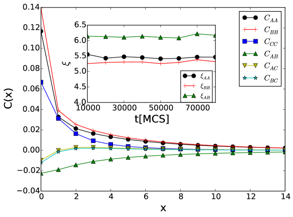
Figure 11: Monte Carlo simulations with direct predator competition. Main panel: Quasi-stationary correlation functions $C(x)$ after the system has evolved for $10\,000$ MCS with $\omega_{\mu A}=0.147$, $\omega_{\eta A}=0.1$, $\omega_{\eta B}=0.15$, and $\omega_{\mu B}=0.1$, when the system resides in the coexistence state. Inset: temporal evolution of the correlation length $\xi(t)$; all lengths are measured in units of the square lattice spacing.

It is of interest to study the spatial properties of the particle distribution. We choose $\omega_{\mu A}=0.147$ so that the system resides deep in the three-species coexistence region according to Fig. 10. The correlation functions are measured after the system has evolved for $10\,000$ MCS as shown in the main plot of Fig. 11. The results are similar to those in the previous sections in the sense that particles are positively correlated with the ones from the same species, but anti-correlated to individuals from other species. The correlation functions for both predator species are very similar: $C_{AA}(x)$ and $C_{BB}(x)$ overlap each other for $x\geq 5$, and $C_{AC}$ and $C_{BC}$ coincide for $x\geq 2$ lattice sites. The inset displays the measured characteristic correlation length as functions of simulation time, each of which varies on the scale of $\sim 0.1$ during $70\,000$ MCS, indicating that the species clusters maintain nearly constant sizes and keep their respective distances almost unchanged throughout the simulations. The correlation lengths $\xi_{AA}$ and $\xi_{BB}$ are very close and differ only by less than $0.2$ lattice sites. These data help to us to visualize the spatial distribution of the predators: The individuals of both $A$ and $B$ species arrange themselves in clusters with very similar sizes throughout the simulation, and their distances to prey clusters are almost the same as well. Hence predator species $A$ and $B$ are almost indistinguishable in their spatial distribution.

4.3 Monte Carlo simulation results in a zero-dimensional system

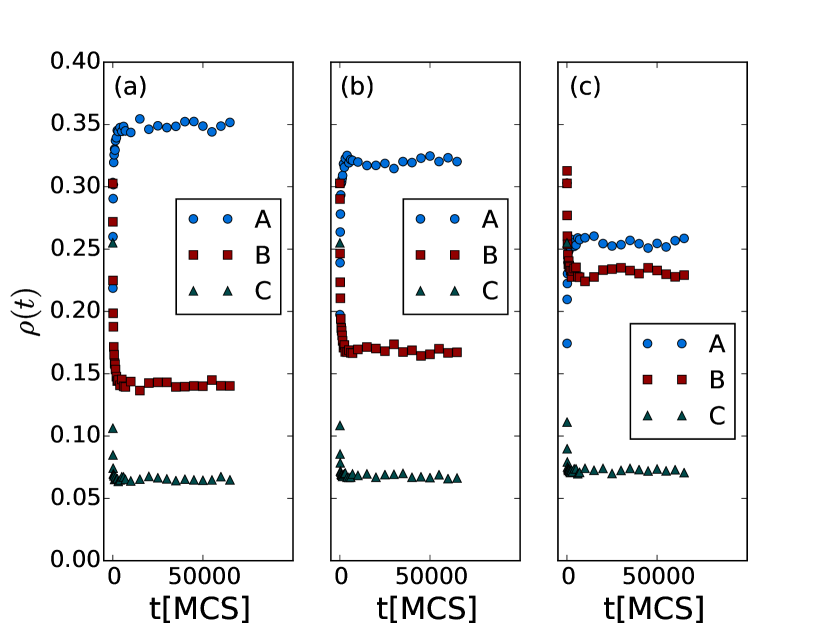
Figure 12: Data obtained from single Monte Carlo simulation runs in a zero-dimensional system with direct competition and evolutionary dynamics, hence only temporal but no spatial correlations: Time record of the population densities for all three species with $\omega_{\eta A}=0.1$, $\omega_{\eta B}=0.15$, $\omega_{\mu B}=0.1$ and $\omega_{\mu A}=0.132,0.140,0.160$ (from left to right), with species $A$ indicated with blue dots, $B$ red-dashed, and $C$ with green triangles.

The above simulations were performed on a two-dimensional system by locating the particles on the sites of a square lattice. Randomly picked particles are allowed to react (predation, reproduction) with their nearest neighbors. Spatial as well as temporal correlations are thus incorporated in the reaction processes. In this subsection, we wish to compare our results with a system for which spatial correlations are absent, yet which still displays manifest temporal correlations. To simulate this situation, we remove the nearest-neighbor restriction and instead posit all particles in a ‘zero-dimensional’ space. In the resulting ‘urn’ model, the simulation algorithm entails to randomly pick two particles and let them react with a probability determined by their individual character values. We find that if all the particles from a single species are endowed with homogeneous properties, i.e., the reaction rates are fixed and uniform as in section 2, no three-species coexistence state is ever observed. If evolution is added without direct competition between predator species as in section 3, the coexistence state does not exist neither. Our observation is again that coexistence occurs only when both evolution and direct competition are introduced. Qualitatively, therefore, we obtain the same scenarios as in the two-dimensional spatially extended system. The zero-dimensional system however turns out even more robust than the one on a two-dimensional lattice, in the sense that its three-species coexistence region is considerably more extended in parameter space. Figure 12 displays a series of population density time evolutions from single zero-dimensional simulation runs with identical parameters as in Fig. 9. All graphs in Fig. 12 reside deeply in the three-species coexistence region, while Fig. 9(a) and (c) showed approaches to absorbing states with one of the predator species becoming extinct. With $\omega_{\eta A}=0.1$, $\omega_{\eta B}=0.15$, and $\omega_{\mu B}=0.1$ fixed, three-species coexistence states in the zero-dimensional system are found in the region $\omega_{\mu A}\in(0,1)$, which is to be compared with the much narrower interval $(0.136,0.159)$ in the two-dimensional system, indicating that spatial extent tends to destabilize these systems.

This finding is in remarkable contrast to some already well-studied systems such as the three-species cyclic competition model, wherein spatial extension and disorder crucially help to stabilize the system [43, 44]. Even though we do not allow explicit nearest-neighbor ‘hopping’ of particles in the lattice simulation algorithm, there still emerges effective diffusion of prey particles followed by predators. Since predator individuals only have access to adjacent prey in the lattice model, the presence of one predator species would block their neighboring predators from their prey. Imagining a cluster of predator particles surrounded by the other predator species, they will be prevented from reaching their ‘food’ and consequently gradually die out. However, this phenomenon cannot occur in the zero-dimensional system where no spatial structure exists at all, and hence blockage is absent. In the previous section we already observed that the cluster size of predator species remains almost unchanged throughout the simulation process when the total population size of the weaker predator species gradually decreases to zero, indicating that clusters vanish in a sequential way. We also noticed that population densities reach their quasi-stationary values much faster in the non-spatial model, see Fig. 12, than on the two-dimensional lattice, Fig. 9. In the spatially extended system, particles form intra-species clusters, and reactions mainly occur at the boundaries between neighboring such clusters of distinct species, thus effectively reducing the total reaction speed. This limiting effect is absent in the zero-dimension model where all particles have equal chances to meet each other.

4.4 Character displacements

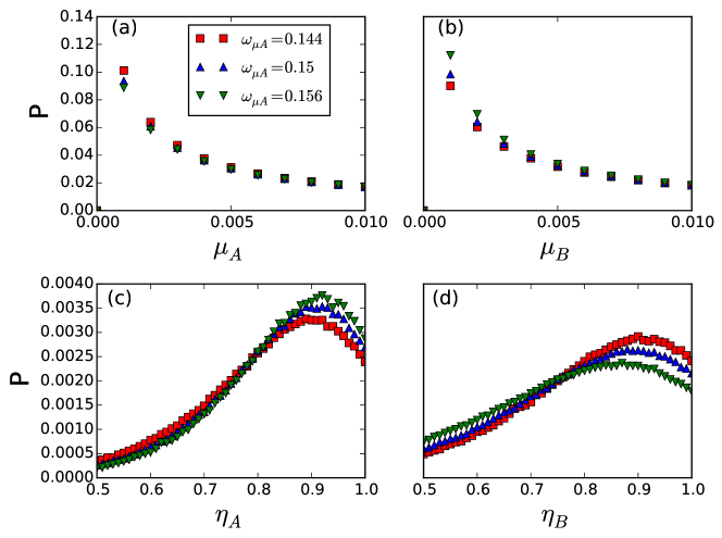
Figure 13: Monte Carlo simulations with direct predator competition: The final distribution of predation efficiencies $\eta$ and predator death rates $\mu$ after the system has stabilized after $50\,000$ MCS with initial distribution widths $\omega_{\eta A}=0.15$, $\omega_{\eta B}=0.1$, $\omega_{\mu B}=0.1$ and $\omega_{\mu A}\in[0.144,0.15,0.156]$; data indicated respectively with red squares, blue triangles up, and green triangles down. (a) and (c) depict the distribution of characters of predator species $A$, while (b) and (d) that of $B$. The interval $[0,1]$ is divided evenly into $1\,000$ histogram bins; the quantity $P$ represents the proportion of individuals with rates in the corresponding bins.

Biologists rely on direct observation of animals’ characters such as beak size when studying trait displacement or evolution [6, 2, 7, 8, 32, 33, 34, 35]. Interspecific competition and natural selection induces noticeable character changes within tens of generations so that the animals may alter their phenotype, and thus look different to their ancestors. On isolated islands, native lizards change the habitat use and move to elevated perches following invasion by a second lizard kind with larger body size. In response, the native subspecies may evolve bigger toepads [45]. When small lizards cannot compete against the larger ones, character displacement aids them to exploit new living habitats by means of developing larger toepads in this case, as a result of natural selection.

Interestingly, we arrive at similar observations in our model, where predation efficiencies $\eta$ and death rates $\mu$ are allowed to be evolving features of the individuals. In Fig. 13, the predation efficiency $\eta$ is initially uniformly set to $0.5$ for all particles, and the death rate $\mu=0.5$ for all predators (of either species). Subsequently, in the course of the simulations the values of any offspring’s $\eta$ and $\mu$ are selected from a truncated Gaussian distribution centered at their parents’ characters with distribution width $\omega_{\eta}$ and $\omega_{\mu}$. When the system arrives at a final steady state, the values of $\eta$ and $\mu$ too reach stationary distributions that are independent of the initial conditions. We already demonstrated above that smaller widths $\omega$ afford the corresponding predator species advantages over the other, as revealed by a larger and stable population density. In Fig. 13, we fix $\omega_{\eta A}=0.15$, $\omega_{\eta B}=0.1$, $\omega_{\mu B}=0.1$, and choose values for $\omega_{\mu A}\in[0.144,0.15,0.156]$ (represented respectively by red squares, blue triangles up, and green triangles down), and measure the final distribution of $\eta$ and $\mu$ when the system reaches stationarity after $50\,000$ MCS. Figures 13(a) and (c) show the resulting distributions for predator species $A$, while (b) and (d) those for $B$. Since both $\mu$ and $\eta$ are in the range $[0,1]$, we divide this interval evenly into $1\,000$ bins, each of length $0.001$. The distribution frequency $P$ is defined as the number of individuals whose character values fall in each of these bins, divided by the total particle number of that species. In Fig. 13(a), the eventual distribution of $\mu_{A}$ is seen to become slightly less optimized as $\omega_{\mu A}$ is increased from $0.144$ to $0.156$ since there is a lower fraction of low $\mu_{A}$ values in the green curve as compared with the red one. Since species $A$ has a larger death rate, its final stable population density decreases as $\mu_{A}$ increases. In parallel, the distribution of $\eta_{A}$ becomes optimized as shown in Fig. 13(c), as a result of natural selection: Species $A$ has to become more efficient in predation to make up for its disadvantages associated with its higher death rates. Predator species $B$ is also influenced by the changes in species $A$. Since there is reduced competition from $A$ in the sense that its population number decreases, the $B$ predators gain access to more resources, thus lending its individuals with low predation efficiencies better chances to reproduce, and consequently rendering the distribution of $\eta_{B}$ less optimized, see Fig. 13(d). This observation can be understood as predator species $B$ needs no longer become as efficient in predation because they enjoy more abundant food supply. In that situation, since species $B$ does not perform as well as before in predation, their death rate $\mu_{B}$ distribution in turn tends to become better optimized towards smaller values, as is evident in Fig. 13(b).

4.5 Periodic environmental changes

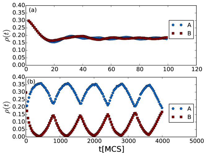
Figure 14: Monte Carlo simulations showing the temporal record of both predator population densities when the distribution widths $\omega_{\eta A}$ and $\omega_{\eta B}$ periodically exchange their values between $0.2$ and $0.3$. The other parameters are set to $\mu_{A}=\mu_{B}=0.125$, $\sigma=1.0$, and $\omega_{C}=\omega_{\mu A}=\omega_{\mu B}=0$. The switch periods are $T=10$ MCS in (a) and $T=400$ MCS in (b).

Environmental factors also play an important role in population abundance. There already exist detailed computational studies of the influence of spatial variability on the two-species lattice LV model [43, 31, 37]. However, rainfall, temperature, and other weather conditions that change in time greatly determine the amount of food supply. A specific environmental condition may favor one species but not others. For example, individuals with larger body sizes may usually bear lower temperatures than small-sized ones. Since animals have various characters favoring certain natural conditions, one may expect environmental changes to be beneficial for advancing biodiversity.

We here assume a two-predator system with species $A$ stronger than $B$ so that the predator $B$ population will gradually decrease as discussed in section 3. Yet if the environment changes and turns favorable to species $B$ before it goes extinct, it may be protected from extinction. According to thirty years of observation of two competing finch species on an isolated island ecology [32], there were several instances when environmental changes saved one or both of them when they faced acute danger of extinction. We take $\omega_{\eta A}$ and $\omega_{\eta B}$ as the sole control parameters determining the final states of the system, holding all other rates fixed in our model simulations. Even though the environmental factors cannot be simulated directly here, we may effectively address environment-related population oscillations by changing the predation efficiency distribution widths $\omega$. We initially set $\omega_{\eta A}=0.2$ and $\omega_{\eta B}=0.3$, with the other parameters held constant at $\mu_{A}=\mu_{B}=0.125$, $\sigma=1.0$, and $\omega_{C}=\omega_{\mu A}=\omega_{\mu B}=0$. In real situations the environment may alternate stochastically; in our idealized scenario, we just exchange the values of $\omega_{\eta A}$ and $\omega_{\eta B}$ periodically for the purpose of simplicity. The population average of the spontaneous death rate is around $0.02$, therefore its inverse $\approx 50$ MCS yields a rough approximation for the individuals’ typical dwell time on the lattice. When the time period $T$ for the periodic switches is chosen as $10$ MCS, which is shorter than one generation’s life time, the population densities remain very close to their identical mean values, with small oscillations; see Fig. 14(a). Naturally, neither species faces the danger of extinction when the environmental change frequency is high. In Fig. 14(b), we study the case of a long switching time $T=400$ MCS, or about eight generations. As one would expect, the $B$ population abundance decreases quickly within the first period. Before the $B$ predators reach total extinction, the environment changes to in turn rescue this species $B$. This example shows that when the environment stays unaltered for a very long time, the weaker species that cannot effectively adapt to this environment would eventually vanish while only the stronger species would survive and strive. When the time period $T$ close matches the characteristic decay time $t_{c}$, see Fig. 14(b), one observes a resonant amplification effect with large periodic population oscillations enforced by the external driving.

5 Summary

In this paper, we have used detailed Monte Carlo simulations to study an ecological system with two predator and one prey species on a two-dimensional square lattice. The two predator species may be viewed as related families, in that they pursue the same prey and are subject to similar reactions, which comprise predation, spontaneous death, and (asexual) reproduction. The most important feature in this model is that there exists only one mobile and reproducing food resource for all predators to compete for. We have designed different model variants with the goal of finding the key properties that could stabilize a three-species coexistence state, and thus facilitate biodiversity in this simple idealized system. We find no means to obtain such coexistence when all reaction rates are fixed or individuals from the same species are all homogeneous, which clearly indicates the importance of demographic variability and evolutionary population adaptation. When dynamical optimization of the individuals in the reproduction process is introduced, they may develop various characters related to their predation and reproduction efficiencies. However, this evolutionary dynamics itself cannot stabilize coexistence for all three species, owing to the fixed constraint that both predator kinds compete for the same food resource. In our model, direct competition between predator species is required to render a three-species coexistence state accessible, demonstrating the crucial importance of combined mutation, competition, and natural selection in stabilizing biodiversity.

We observe critical slowing-down of the population density decay near the predator extinction thresholds, which also serves as an indicator to locate the coexistence region in parameter space. When the system attains its quasi-steady coexistence state, the spatial properties of the particle distribution remain stable even as the system evolves further. Character displacements hence occur as a result of inter-species competition and natural selection in accord with biological observations and experiments. Through comparison of the coexistence regions of the full lattice model and its zero-dimensional representation, we find that spatial extent may in fact reduce the ecosystem’s stability, because the two predator species can effectively block each other from reaching their prey. We also study the influence of environmental changes by periodically switching the rate parameters of the two competing predator species. The system may then maintain three-species coexistence if the period of the environmental changes is smaller than the relaxation time of the population density decay. Matching the switching period to the characteristic decay time can induce resonantly amplified population oscillations.

Stable coexistence states with all three species surviving with corresponding constant densities are thus only achieved through introducing both direct predator competition as well as evolutionary adaptation in our system. In sections 3 and 4, we have explored character displacement without direct competition as well as competition without character displacement, yet a stable three-species coexistence state could not be observed in either case. Therefore it is necessary to include both direct competition and character displacement to render stable coexistence states possible in our model. However, both predator species $A$ and $B$ can only coexist in a small parameter interval for their predation efficiency distribution widths $\omega$, because they represent quite similar species that compete for the same resources. In natural ecosystems, of course other factors such as distinct food resources might also help to achieve stable multi-species coexistence.

References

References

- [1] C. R. Darwin, 1859, On the origin of species by means of natural selection, John Murray
- [2] W. L. Brown, E. O. Wilson, 1956, Character displacement, Systematic Zoology, 5, 49–64
- [3] D. Schluter, J. D. McPhail, 1992, Ecological character displacement and speciation in sticklebacks, American Naturalist, 140, 85–108
- [4] M. L. Taper, T. J. Case, 1992, Coevolution among competitors, Oxford Surveys in Evolutionary Biology, 8, 63–109
- [5] J. Melville, 2002, Competition and character displacement in two species of scincid lizards, Ecology letters, 5, 386–393
- [6] D. Lack, 1947, Darwin’s finches, Cambridge University Press
- [7] P. R. Grant, 1975, The classic case of character displacement, Evolutionary Biology, 8, 237
- [8] W. Arthur, 1982, The evolutionary consequences of interspecific competition, Advances in Ecological Research, 12, 127–87
- [9] J. Maynard Smith, 1982, Evolution and the theory of games, Cambridge University Press
- [10] A. J. Lotka, 1920, Undamped oscillations derived from the law of mass action, Journal of the American Chemical Society, 42, 1595
- [11] V. Volterra, 1926, Fluctuations in the abundance of a species considered mathematically, Nature, 118, 558
- [12] H. Matsuda, N. Ogita, A. Sasaki and K. Satō, 1992, Statistical mechanics of population – the lattice Lotka-Volterra model, Progress of Theoretical Physics, 88, 1035–1049
- [13] J. E. Satulovsky and T. Tomé, 1994, Stochastic lattice gas model for a predator-prey system, Physical Review E, 49, 5073
- [14] N. Boccara, O. Roblin and M. Roger, 1994, Automata network predator-prey model with pursuit and evasion, Physical Review E, 50, 4531
- [15] R. Durrett, 1999, Stochastic spatial models, SIAM Review, 41, 677–718
- [16] A. Provata, G. Nicolis and F. Baras, 1999, Oscillatory dynamics in low-dimensional supports: a lattice Lotka-Volterra model, Journal of Chemical Physics, 110, 8361
- [17] A. F. Rozenfeld, E. V. Albano, 1999, Study of a lattice-gas model for a prey-predator system, Physica A, 266, 322–329
- [18] A. Lipowski, 1999, Oscillatory behavior in a lattice prey-predator system, Physical Review E, 60, 5179
- [19] A. Lipowski, D. Lipowska, 2000, Nonequilibrium phase transition in a lattice prey-predator system, Physica A, 276, 456–464
- [20] R. Monetti, A. Rozenfeld, E. Albano, 2000, Study of interacting particle systems: the transition to the oscillatory behavior of a prey-predator model, Physica A, 283, 52
- [21] M. Droz, A. Pȩkalski, 2001, Coexistence in a predator-prey system, Physical Review E, 63, 051909
- [22] T. Antal, M. Droz, 2001, Phase transitions and oscillations in a lattice prey-predator model, Physical Review E, 63, 056119
- [23] M. Kowalik, A. Lipowski, A. L. Ferreira, 2002, Oscillations and dynamics in a two-dimensional prey-predator system, Physical Review E, 66, 066107
- [24] M. Mobilia, I. T. Georgiev, U. C. Täuber, 2006, Fluctuations and correlations in lattice models for predator-prey interaction, Physical Review E, 73, 040903
- [25] M. Mobilia, I. T. Georgiev, U. C. Täuber, 2006, Phase transitions and spatio–temporal fluctuations in stochastic lattice Lotka-Volterra models, Journal of Statistical Physics, 128, 447
- [26] M. J. Washenberger, M. Mobilia, U. C. Täuber, 2007, Influence of local carrying capacity restrictions on stochastic predator-prey models, Journal of Physics: Condensed Matter, 19, 065139
- [27] S. Chen, U. C. Täuber, 2016, Non-equilibrium relaxation in a stochastic lattice Lotka-Volterra model, Physical Biology, 13, 025005
- [28] L. Frachebourg, P. L. Krapivsky, and E. Ben-Naim, 1996, Spatial organization in cyclic Lotka-Volterra systems, Physical Review Letter, 77, 2125
- [29] H. Y. Shih, N. Goldenfeld, 2014, Path-integral calculation for the emergence of rapid evolution from demographic stochasticity, Physical Review E, 90, 050702
- [30] U. Dobramysl, M. Mobilia, M. Pleimling, U. C. Täuber, 2017, Stochastic population dynamics in spatially extended predator-prey systems, to appear in Journal of Physics A: Mathematical and Theoretical [arXiv:1708.07055]
- [31] U. Dobramysl, U. C. Täuber, 2013, Environmental versus demographic variability in two-species predator-prey models, Physical Review Letter, 110, 048105
- [32] P. R. Grant, B. R. Grant, 2006, Evolution of Character Displacement in Darwin’s finches, Science, 313, 224–226
- [33] A. M. Rice, A. R. Leichty, D. W. Pfennig, 2009, Parallel evolution and ecological selection: replicated character displacement in spadefoot toads, Proceedings of the Royal Society B, 276, 4189–4196
- [34] Y. E. Stuart, T. S. Campbell, P. A. Hohenlohe, R. G. Reynolds, L. J. Revell, J. B. Losos, 2014, Rapid evolution of a native species following invasion by a congener, Science, 346, 463–466
- [35] J. Tan, M. R. Slattery, X. Yang, L. Jiang, 2016, Phylogenetic context determines the role of competition in adaptive radiation, Proceedings of the Royal Society B, 283
- [36] P. Grassberger, Y-C Zhang, 1996, Self-organized formulation of standard percolation phenomena Physica A, 224, 169
- [37] U. Dobramysl, U. C. Täuber, 2013, Environmental versus demographic variability in stochastic predator-prey models, Journal of Statistical Mechanics, 2013, P10001
- [38] S. R. Broadbent, J. M. Hammersley, 1957, Percolation Processes, Mathematical Proceedings of the Cambridge Philosophical Society, 53, 629
- [39] M. Henkel, H. Hinrichsen, S. Lübeck, 2008, Non-equilibrium phase transitions vol 1: Absorbing phase transitions (Bristol, UK: Springer)
- [40] U. C. Täuber, 2014, Critical dynamics – A field theory approach to equilibrium and non-equilibrium scaling behavior (Cambridge: Cambridge University Press)
- [41] C. A. Voigt, R. M. Ziff, 1997, Epidemic analysis of the second-order transition in the Ziff-Gulari-Barshad surface-reaction model, Physical Review E, 56, R6241
- [42] L. Dai, D. Vorselen, K. S. Korolev, J. Gore, 2012, Generic indicators for loss of resilience before a tipping point leading to population collapse, Science, 336, 1175
- [43] U. Dobramysl, U. C. Täuber, 2008, Spatial variability enhances species fitness in stochastic predator-prey interactions, Physical Review Letter, 101, 258102
- [44] Q. He, M. Mobilia, U. C. Täuber, 2011, Coexistence in the two-dimensional May–Leonard model with random rates, European Physical Journal B, 82, 97 - 105
- [45] S. Y. Strauss, J. A. Lau, T. W. Schoener, P. Tiffin, 2008, Evolution in ecological field experiments: implications for effect size, Ecology Letters, 11, 199–207