Static Orbits in Rotating Spacetimes

Abstract

We show that under certain conditions an axisymmetric rotating spacetime contains a ring of points in the equatorial plane, where a particle at rest with respect to an asymptotic static observer remains at rest in a static orbit. We illustrate the emergence of such orbits for boson stars. Further examples are wormholes, hairy black holes and Kerr-Newman solutions.

I Introduction

Our understanding of the properties of spacetimes largely rests on the analysis of their geodesics. Therefore the study of geodesics has been in the focus of gravity research from its early beginnings. Indeed, describing the motion of particles and light, geodesics rapidly established General Relativity, predicting the observed orbital precession of Mercury and the deflection of light by the sun.

In recent years the study of the orbits of stars around Sgr A^∗ provided strong evidence for a supermassive compact central object at the center of the Milky Way, while observations with the EHT should soon provide us with an image of this object, i.e., presumably the shadow of a supermassive black hole Eckart:2017bhq .

The orbits around Kerr black holes are well-known Chandrasekhar:1985kt . In contrast, much less is known about the orbits in spacetimes of other compact rotating objects, such as boson stars, wormholes or hairy black holes. If such objects were to represent serious contenders for compact astrophysical objects, the presence of unique signatures - not present for Kerr black holes - would be highly valuable for their possible identification.

Here we would like to point out such a feature, which is found in a number of rotating non-Kerr spacetimes. To this end, let us consider a spacetime with a gravitational potential, which has a minimum somewhere in a physically accessible region (e.g., outside an event horizon or a wormhole throat). Since the spacetime is rotating, there is frame dragging. Thus a zero angular momentum particle would be rotating along with the spacetime, and so would a particle with positive angular momentum. However, a particle with negative angular momentum might just stand still with respect to an asymptotic static observer, if its angular momentum would have precisely the right value, and its radial location would correspond to a minimum in the potential.

In the following we briefly recall the geodesic equations in the equatorial plane for a general rotating metric and analyze the conditions necessary to have such static orbits, where massive particles initially at rest remain at rest for all times. In particular, we exemplify this mechanism for rotating boson stars, and point out further examples of spacetimes with static orbits, before we conclude.

II Equatorial geodesics

Consider an axisymmetric, rotating spacetime, where the metric coefficients are functions of $r$ and $\theta$. In the equatorial plane the line element can be chosen as

$$ds^{2}=-Adt^{2}-2Bdtd\varphi+Ddr^{2}+Cd\varphi^{2},$$ (1)

where $A$, $B$, $C$ and $D$ are then only functions of the radial coordinate $r$. The action of a test particle moving in this spacetime is given by

$$S=\frac{1}{2}\int g_{\mu\nu}u^{\mu}u^{\nu}d\tau,$$ (2)

which yields the equations of motion in the equatorial plane. The coordinates $t$ and $\varphi$ are cyclic, leading to two first integrals, identified as the energy per unit mass and the angular momentum per unit mass of the test particle as measured at spatial infinity, namely

$$E=A\dot{t}+B\dot{\varphi};\qquad L=-B\dot{t}+C\dot{\varphi}.$$ (3)

For the equation of motion for the $r$ coordinate we can employ the four-velocity norm instead, $u^{\mu}u_{\mu}=-1$, which yields

$$\dot{r}^{2}=\frac{C}{\Delta D}\left(E-V_{+}\right)\left(E-V_{-}\right),$$ (4)

with the effective potential

$$V_{\pm}=\frac{BL\pm\sqrt{\Delta\left(C+L^{2}\right)}}{C},$$ (5)

and $\Delta=AC+B^{2}$. Note that in the absence of ergoregions $V_{-}$ is always negative. For our purposes it will be sufficient in the following to only consider $V_{+}$. From eq. (3) we can similarly obtain

$$\dot{\varphi}=\frac{B}{\Delta}\left(E-V_{\varphi}\right),$$ (6)

where for convenience we introduce an angular potential $V_{\varphi}=-AL/B$.

III Orbits starting from rest

The Lense-Thirring effect makes it interesting to analyze what happens to particles which are initially at rest. To accomplish this, the particle must be placed at a point, where $E=V_{+}=V_{\varphi}$, so that both $\dot{r}$ and $\dot{\varphi}$ are zero. At this point,

$$\sqrt{A}|_{r_{st}}=E,\quad B|_{r_{st}}=-EL.$$ (7)

Let us now take a rotating boson star as an example to illustrate such orbits of massive particles starting from rest. (See e.g. Liebling:2012fv for a recent review on boson stars. Orbits in boson star spacetimes have been considered e.g. in Eilers:2013lla ; Grandclement:2014msa ; Meliani:2015zta ; Grandclement:2016eng ; Grould:2017rzz ; Meliani:2017ktw .) For the particular example, we choose a boson star without self-interaction with a boson mass $m_{b}=\sqrt{1.1}$, a boson frequency $\omega_{s}=0.84$, and a rotational quantum number $m=1$.

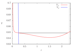
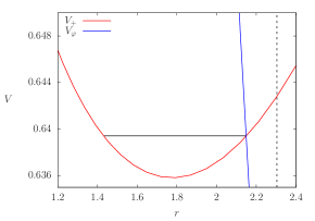
Figure 1: Effective potential $V_{+}$ (red) and angular potential $V_{\varphi}$ (blue). The horizontal solid lines (black) represent the particle energy $E$. The intersection points with the potentials delimit the radial domain of the bound orbit. The vertical dashed lines (black) indicate the location of the maximum value of the boson field. Left: Particle with $L=0.01$. Its starting rest position is located to the left of the minimum of $V_{+}$. Right: Particle with $L=0.5$. Its starting rest position is located to the right of the minimum of $V_{+}$.

Figure 1 shows the effective potential $V_{+}$ together with the angular potential $V_{\varphi}$ for two values of the particle angular momentum $L$, for which eqs. (7) hold. Thus the particle energy $E$ is such that the particle starts from rest, and the domain of its radial motion corresponds to the horizontal line. When the motion starts from rest for a radial coordinate $r_{st}<r_{min}$, where $r_{min}$ denotes the minimum of the potential, the particle is pushed away from the center and engages in the semi orbit, co-rotating with the star, having the largest angular velocity (absolute value) at the apocenter and being at rest at the pericenter. When the motion starts from rest for a radial coordinate $r_{st}>r_{min}$, the particle is pulled towards the center and retains a pointy petal orbit, counter-rotating with respect to the star and having the largest angular velocity (absolute value) at the pericenter, while being at rest at the apocenter. Note, that the occurrence of semi orbits and pointy petal orbits was observed in Grandclement:2014msa ; Grould:2017rzz .

IV Orbits remaining at rest

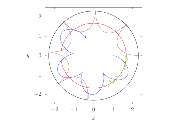
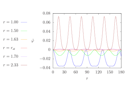
Figure 2: Orbits of massive particles released from rest at different values of the radial coordinate $r$ (and $\varphi=0$) and evolved for the proper time interval $\Delta\tau=180$. The closer the starting point $r$ is to the static ring $r_{st}$ (red circle), the smaller is the amplitude in $\dot{\varphi}$. The maximum of the scalar field is also indicated (black ring).

We illustrate several orbits starting from rest in Fig. 2 for the same boson star solution. These orbits start at different values of the radial coordinate always from $\varphi=0$, and are evolved for the same amount of elapsed proper time $\Delta\tau$. Besides the orbits the oscillating behaviour of $\dot{\varphi}$ is also exhibited (versus the proper time) in Fig. 2.

As we increase the starting value of $r$, the orbits change from co-rotating semi orbits to counter-rotating pointy petal orbits. Clearly, in between there arises a critical value of $r$, $r_{st}=1.6753373$. At this value a static particle remains static for all times. Therefore $r_{st}$ represents the static orbit ring. The occurrence of this static ring is seen from the figure. The closer the particle starts from the static orbit ring the smaller is its angular displacement during the time $\Delta\tau$, and the smaller is its radial amplitude around the critical point $r_{st}=1.6753373$. Thus in the limit $r\to r_{st}$ the particle remains at rest.

In this case the above condition (7) is met together with the circular orbit condition, namely $\partial_{r}V_{+}=0$. But then instead of exhibiting circular motion the particle will remain at rest in a static orbit at a distance $r_{st}$ from the center. Since the relations (7) combined with the circular orbit condition yield $\partial_{r}V_{+}=\partial_{r}A/(2E)$, a sufficient and necessary condition for a spacetime to allow for a stable (unstable) static orbit ring in its equatorial plane is therefore that its metric component $g_{tt}$ presents a maximum (minimum) anywhere in this plane, $\partial_{r}A=0$, where $g_{tt}<0$.

Fig. 2 also shows, that the static orbits (red circle) are located in the star’s interior, i.e., inside the radius where the scalar field assumes its maximum value (black circle). Thus, if a particle is at rest at $r_{st}$ with respect to an asymptotic static observer, it will remain at rest at all times, provided only the gravitation interaction between this particle and the boson star is taken into account.

To guarantee that this feature is independent of the chosen parametrization, we need to assure that $d\varphi/dr=\dot{\varphi}/\dot{r}=0$ at this point. In order to do so, we analyze this ratio at a point near the static radius by obtaining the ratio of the respective radially perturbed quantities, namely $\delta\dot{\varphi}/\delta\dot{r}$. We define,

$$V_{+}=E+\delta V_{+};\quad V_{\varphi}=E+\delta V_{\varphi};\quad A=A_{st}+\delta A;\quad B=B_{st}+\delta B;\quad C=C_{st}+\delta C;\quad D=D_{st}+\delta D.$$ (8)

From equations (4) and (6) we see that

$$\frac{\delta\dot{\varphi}}{\delta\dot{r}}\propto\frac{\delta V_{\varphi}}{\sqrt{\delta V_{+}}}=\frac{\delta A/E-\delta BE/B}{\sqrt{\delta A/(2E)}}\propto\sqrt{r-r_{st}}.$$ (9)

Let us now consider circumstances, under which such static rings may occur. Clearly, stars whose density maximum is located away from the center represent possible candidates, with rotating boson stars providing the perfect stage for this phenomenon to occur: They only interact gravitationally with ordinary matter and their energy density distribution is toroidal when rotating.

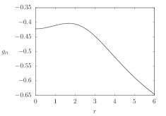
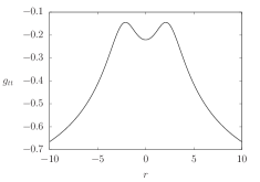
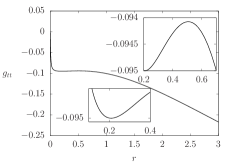
Figure 3: The $g_{tt}$ component for three different systems containing bosonic matter. Left: A pure rotating boson star (without self-interaction). Center: A traversable rotating wormhole immersed in bosonic matter. Right: A rotating black hole with scalar hair.

To pinpoint the presence of this phenomenon, let us inspect the $g_{tt}$ component of several rotating spacetimes. In Fig. 3 we compare the $g_{tt}$ component of three rotating spacetimes, all of which contain a complex scalar field: a boson star, a traversable wormhole immersed in bosonic matter and a hairy black hole. The boson star features a local maximum of $g_{tt}$, corresponding to a local minimum of the effective potential $V_{+}$, where a test particle might be trapped at rest. The solution depicted corresponds to the one analyzed above. However, this feature is rather generic for boson star solutions, arising also for quartic and sixtic self-interaction potentials Kleihaus:2005me ; Kleihaus:2007vk ; Kleihaus:2011sx as well as for rotationally and radially excited boson stars Collodel:2017biu .

The rotating wormhole solution contains a phantom field besides the complex scalar field, which in the example depicted is non-interacting Hoffmann:2017 . Such solutions represent rotating generalizations of the wormhole solutions studied in Dzhunushaliev:2014bya . The metric function $g_{tt}$ exhibited in Fig. 3 contains three local extrema, two symmetric maxima and a minimum at the throat (at $r=0$). It is thus possible to have particles at (unstable) rest exactly at the throat in between the two universes and also at (stable) rest at a certain position $\pm r_{st}$ in each of the universes.

Rotating black holes carrying complex scalar field hair arise for a non-interacting boson field as well as in the case of self-interaction Herdeiro:2014goa ; Kleihaus:2015iea ; Herdeiro:2015tia . As seen in the figure, for a sufficiently small horizon radius, the metric function $g_{tt}$ features both a local maximum and a local minimum, possessing thus two static orbit rings, one stable and one unstable, respectively. The hairy black hole depicted is based on a quartic potential Kleihaus:2015iea . Note, that the radial coordinate in the figure is shifted such that the horizon radius is located $r_{H}=0$.

The static orbit ring is, however, not an exclusive feature of spacetimes warped by a spin-0 field. The $g_{tt}$ component of the well known Kerr-Newman solution also contains a local maximum at $r_{st}=Q^{2}/M$. Not only is this radius independent of the angular momentum but is also present at the same location in the non-rotating Reissner-Nordström solution. Surprisingly, the authors could not find any reference to these findings in the literature. We emphasize that the equations of motion are geodesics, namely for test particles without electric charge. The close relation between $g_{tt}$ and the energy per unit mass of the orbiting particle, eq. (7), demands a more careful analysis for these spacetimes. The only possible observational scenario is that of a naked singularity, where the static ring is always present, whether there is rotation or not. However, when the solution is a black hole, the static ring is always hidden behind the event horizon. Static rings are located behind both horizons if $J^{2}\geq\alpha^{2}-\alpha^{4}$, where $J$ is the black hole’s angular momentum and $\alpha=Q/M$. By writing $J^{2}=\alpha^{2}(1-\alpha^{2})+\delta$, with $\delta\geq 0$, we obtain $\alpha^{2}\leq 1-\sqrt{\delta}$ as a further constraint on the charge. The static ring is also found in the presence of charged black holes in higher dimensions. The five dimensional Breckenridge-Myers-Peet-Vafa (BMPV) spacetime (for details on the geodesics see Gibbons:1999uv ; Herdeiro:2000ap ; Diemer:2013fza ) possesses two orthogonal rings (parametrized by $\varphi$ and $\psi$) at $r_{st}=\sqrt{\mu}$, where $\mu$ is again a parameter that depends only on the mass and charge.

V Conclusions

We have shown that under specific conditions a rotating spacetime may possess a ring in the equatorial plane, where massive particles initially at rest with respect to an asymptotic static observer remain at rest. It is worth mentioning that this phenomenon of static orbits is a purely inertial one. (This is in contrast to the equilibrium positions found for charged particles orbiting charged black holes.)

The physical conditions to be met in order to allow for such static orbits require, that besides a precise balance between the angular momentum and the frame dragging, the gravitational potential contained in the metric component $g_{tt}$ should possess a minimum, such that a particle sitting at the corresponding radius $r_{st}$ is neither pulled towards the center nor pushed away from it. Clearly, the extremum of $g_{tt}$ and the extremum of the effective potential must therefore coincide at $r_{st}$.

Let us note that somewhat similar conditions are found for null geodesics Grandclement:2016eng . Here, the presence of so-called static light points, requires furthermore that their spatial location coincides with the onset or termination of an ergoregion, $A|_{r_{st}}=0$, and that the photons have zero energy.

While we have exemplified our analysis in detail for boson stars, we have shown, that static orbits arise not only for boson stars but also for Ellis wormholes immersed in rotating bosonic matter, as well as for hairy black holes or Kerr-Newman solutions.

While one might argue that it might be unlikely to expect nature to produce such a fine tuned scenario, we have verified that geodesics followed by particles initially at rest near the (stable) static radius are characterized by slow motion. The closer they start from $r_{st}$ the smaller are their maximal radial and angular velocities. This opens the possibility of observing this phenomenon, if rotating compact objects such as the above examples would indeed exist in nature.

Therefore, observing static, or quasi-static, astrophysical objects in a region which otherwise indicates the presence of a strong gravitational field could offer support for the presence of a type of compact object that differs from Kerr black holes.

VI Acknowledgments

We would like to acknowledge support by the DFG Research Training Group 1620 Models of Gravity as well as by FP7, Marie Curie Actions, People, International Research Staff Exchange Scheme (IRSES-606096), COST Action CA16104 GWverse. BK gratefully acknowledges support from Fundamental Research in Natural Sciences by the Ministry of Education and Science of Kazakhstan.

References

- (1) A. Eckart et al., Found. Phys. 47, 553 (2017) doi:10.1007/s10701-017-0079-2
- (2) S. Chandrasekhar, “The mathematical theory of black holes,” (Oxford, UK, Clarendon (1985))
- (3) S. L. Liebling and C. Palenzuela, Living Rev. Rel. 15, 6 (2012) doi:10.12942/lrr-2012-6
- (4) V. Diemer, K. Eilers, B. Hartmann, I. Schaffer and C. Toma, Phys. Rev. D 88, 044025 (2013) doi:10.1103/PhysRevD.88.044025
- (5) P. Grandclément, C. Somé and E. Gourgoulhon, Phys. Rev. D 90, 024068 (2014) doi:10.1103/PhysRevD.90.024068
- (6) Z. Meliani, F. H. Vincent, P. Grandclément, E. Gourgoulhon, R. Monceau-Baroux and O. Straub, Class. Quant. Grav. 32, 235022 (2015) doi:10.1088/0264-9381/32/23/235022
- (7) P. Grandclément, Phys. Rev. D 95, 084011 (2017) doi:10.1103/PhysRevD.95.084011
- (8) M. Grould, Z. Meliani, F. H. Vincent, P. Grandclément and E. Gourgoulhon, Class. Quant. Grav. 34, 215007 (2017) doi:10.1088/1361-6382/aa8d39
- (9) Z. Meliani, F. Casse, P. Grandclément, E. Gourgoulhon and F. Dauvergne Class. Quant. Grav. 34, 225003 (2017) doi:10.1088/1361-6382/aa8fb5
- (10) B. Kleihaus, J. Kunz and M. List, Phys. Rev. D 72, 064002 (2005) doi:10.1103/PhysRevD.72.064002
- (11) B. Kleihaus, J. Kunz, M. List and I. Schaffer, Phys. Rev. D 77, 064025 (2008) doi:10.1103/PhysRevD.77.064025
- (12) B. Kleihaus, J. Kunz and S. Schneider, Phys. Rev. D 85, 024045 (2012) doi:10.1103/PhysRevD.85.024045
- (13) L. G. Collodel, B. Kleihaus and J. Kunz, Phys. Rev. D 96, 084066 (2017) doi:10.1103/PhysRevD.96.084066
- (14) C. Hoffmann et al (in preparation).
- (15) V. Dzhunushaliev, V. Folomeev, C. Hoffmann, B. Kleihaus and J. Kunz, Phys. Rev. D 90, 124038 (2014) doi:10.1103/PhysRevD.90.124038
- (16) C. A. R. Herdeiro and E. Radu, Phys. Rev. Lett. 112, 221101 (2014) doi:10.1103/PhysRevLett.112.221101
- (17) B. Kleihaus, J. Kunz and S. Yazadjiev, Phys. Lett. B 744, 406 (2015) doi:10.1016/j.physletb.2015.04.014
- (18) C. A. R. Herdeiro, E. Radu and H. Runarsson, Phys. Rev. D 92, 084059 (2015) doi:10.1103/PhysRevD.92.084059
- (19) G. W. Gibbons and C. A. R. Herdeiro, Class. Quant. Grav. 16, 3619 (1999) doi:10.1088/0264-9381/16/11/311
- (20) C. A. R. Herdeiro, Nucl. Phys. B 582, 363 (2000) doi:10.1016/S0550-3213(00)00335-7
- (21) V. Diemer and J. Kunz, Phys. Rev. D 89,084001 (2014) doi:10.1103/PhysRevD.89.084001