Weak convergence of Galerkin approximations for fractional elliptic stochastic PDEs with spatial white noise

Abstract.

The numerical approximation of the solution to a stochastic partial differential equation with additive spatial white noise on a bounded domain is considered. The differential operator is assumed to be a fractional power of an integer order elliptic differential operator. The solution is approximated by means of a finite element discretization in space and a quadrature approximation of an integral representation of the fractional inverse from the Dunford–Taylor calculus.

For the resulting approximation, a concise analysis of the weak error is performed. Specifically, for the class of twice continuously Fréchet differentiable functionals with second derivatives of polynomial growth, an explicit rate of weak convergence is derived, and it is shown that the component of the convergence rate stemming from the stochasticity is doubled compared to the corresponding strong rate. Numerical experiments for different functionals validate the theoretical results.

1. Introduction

The representation of Gaussian random fields as solutions to stochastic partial differential equations (SPDEs) has become a popular approach in spatial statistics in recent years. It was observed already in [21] and [22] that a Gaussian random field $u$ on $\mathbb{R}^{d}$ with a covariance function of Matérn type [13] solves an SPDE of the form $(\kappa^{2}-\Delta)^{\beta}u=\mathcal{W}$. Here, $\mathcal{W}$ is Gaussian white noise, $\kappa>0$ is a parameter determining the practical correlation range of the field, and $\beta>d/4$ controls the smoothness parameter $\nu$ of the Gaussian Matérn field via the equality $\nu=2\beta-d/2$.

Later, this relation was the incentive to consider the SPDE

$$(\kappa^{2}-\Delta)^{\beta}u=\mathcal{W}\quad\text{in }\mathcal{D}$$ (1.1)

for Gaussian random field approximations of Matérn fields on bounded domains $\mathcal{D}\subsetneq\mathbb{R}^{d}$. On the boundary $\partial\mathcal{D}$, the operator $\kappa^{2}-\Delta$ is augmented with, e.g., homogeneous Dirichlet or Neumann boundary conditions. In [12] it was shown that by restricting the value of $\beta$ to $2\beta\in\mathbb{N}$ and by solving the stochastic problem (1.1) by means of a finite element method, the computational costs of many operations, which are needed for statistical inference, such as sampling and likelihood evaluations can be significantly reduced. This decrease in computing time is one of the main reasons for the popularity of the SPDE approach in spatial statistics. In addition, it facilitates various extensions of the Matérn model which are difficult to formulate using a covariance-based approach, see, for instance, [2, 5, 10, 12, 20].

However, the constraint $2\beta\in\mathbb{N}$ imposed by [12] restricts the value of the smoothness parameter $\nu$, which is the most important parameter when the model is used for prediction [17]. In [4] we showed that this restriction can be avoided by combining a finite element discretization in space with a quadrature approximation based on an integral representation of the inverse fractional power operator from the Dunford–Taylor calculus. We furthermore derived an explicit rate of convergence for the strong mean-square error of the proposed approximation for a class of fractional elliptic stochastic equations including (1.1).

In practice, it is often not only necessary to sample from the solution $u$ to (1.1), but also to estimate the expected value $\mathbb{E}[\varphi(u)]$ of a certain real-valued quantity of interest $\varphi(u)$. The aim of this work is to provide a concise analysis of the weak error $|\mathbb{E}[\varphi(u)]-\mathbb{E}[\varphi(u_{h,k}^{Q})]|$ for the approximation $u_{h,k}^{Q}$ proposed in [4]. This analysis includes the derivation of an explicit weak convergence rate for twice continuously Fréchet differentiable real-valued functions $\varphi$, whose second derivatives are of polynomial growth. Functions of this form occur in many applications, e.g., when integral means of the solution with respect to a certain subdomain of $\mathcal{D}$ are of interest, or when a transformation of the model is used as a component in a hierarchical model. An example of the latter situation is to consider logit or probit transformed Gaussian random fields for binary regression models [16, §4.3.3].

We prove that, compared to the convergence rate of the strong error formulated in [4], the component of the weak convergence rate stemming from the stochasticity of the problem is doubled. To this end, two time-dependent stochastic processes are introduced, which at time $t=1$ have the same probability distribution as the exact solution $u$ and the approximation $u_{h,k}^{Q}$, respectively. The weak error is then bounded by introducing an associated Kolmogorov backward equation on the interval $[0,1]$ and applying Itô calculus.

The structure of this article is as follows: In §2 we formulate the equation of interest in a Hilbert space setting similarly to [4] and state our main result on weak convergence of the approximation in Theorem 2.4. A detailed proof of Theorem 2.4 is given in §3. For validating the theoretical result in practice, we describe the outcomes of several numerical experiments in §4. Finally, §5 concludes the article with a discussion.

2. Weak approximations

The subject of our investigations is the fractional order equation considered in [4],

$$L^{\beta}u=g+\mathcal{W},$$ (2.1)

for $\beta\in(0,1)$, where $\mathcal{W}$ denotes Gaussian white noise defined on a complete probability space $(\Omega,\mathcal{A},\mathbb{P})$ with values in a separable Hilbert space $H$. Here and below, (in-)equalities involving random terms are meant to hold $\mathbb{P}$-almost surely, if not specified otherwise. Furthermore, we use the notation $X\overset{d}{=}Y$ to indicate that two random variables $X$ and $Y$ have the same probability distribution.

Similarly to [4], we make the following assumptions: $L\colon\mathscr{D}(L)\subset H\to H$ is a densely defined, self-adjoint, positive definite operator and has a compact inverse $L^{-1}\colon H\to H$. In this case, $-L$ generates an analytic strongly continuous semigroup $(S(t))_{t\geq 0}$ on $H$. The $H$-orthonormal eigenvectors of $L$ are denoted by $\{e_{j}\}_{j\in\mathbb{N}}$ and the corresponding eigenvalues by $\{\lambda_{j}\}_{j\in\mathbb{N}}$. These values are listed in nondecreasing order and we assume that there exist constants $\alpha,c_{\lambda},C_{\lambda}>0$ such that

$$c_{\lambda}\,j^{\alpha}\leq\lambda_{j}\leq C_{\lambda}\,j^{\alpha}\qquad\forall j\in\mathbb{N}.$$ (2.2)

The action of the fractional power operator $L^{\beta}$ in (2.1) is well-defined on

$$\dot{H}^{2\beta}:=\mathscr{D}(L^{\beta})=\Bigl{\{}\psi\in H:\|\psi\|_{2\beta}^{2}:=\|L^{\beta}\psi\|_{H}^{2}=\sum_{j\in\mathbb{N}}\lambda_{j}^{2\beta}(\psi,e_{j})_{H}^{2}<\infty\Bigr{\}},$$

which is itself a Hilbert space with inner product $(\phi,\psi)_{2\beta}:=(L^{\beta}\phi,L^{\beta}\psi)_{H}$. Furthermore, there exists a unique continuous extension of $L^{\beta}$ to an isometric isomorphism $L^{\beta}\colon\dot{H}^{r}\to\dot{H}^{r-2\beta}$ for all $r\in\mathbb{R}$, see [4, Lem. 2.1]. Here, for $s>0$, the negative-indexed space $\dot{H}^{-s}$ is defined as the dual space of $\dot{H}^{s}$. After identifying the dual space $H^{*}$ of $\dot{H}^{0}:=H$ via the Riesz map, we obtain the Gelfand triple $\dot{H}^{s}\hookrightarrow H\cong H^{*}\hookrightarrow\dot{H}^{-s}$ with continuous and dense embeddings. The norm on the dual space $\dot{H}^{-s}$ can be expressed by

$$\|g\|_{-s}=\sup\limits_{\phi\in\dot{H}^{s}\setminus\{0\}}\frac{\langle g,\phi\rangle}{\|\phi\|_{s}}=\biggl{(}\sum_{j\in\mathbb{N}}\lambda_{j}^{-s}\langle g,e_{j}\rangle^{2}\biggr{)}^{\frac{1}{2}},$$

where $\langle\,\cdot\,,\,\cdot\,\rangle$ denotes the duality pairing on $\dot{H}^{-s}$ and $\dot{H}^{s}$, [19, Proof of Lem. 5.1]. With this representation of the dual norm and the growth (2.2) of the eigenvalues $\lambda_{j}$ at hand, it is an immediate consequence of a Karhunen–Loève expansion of the white noise $\mathcal{W}$ with respect to the $H$-orthonormal eigenvectors $\{e_{j}\}_{j\in\mathbb{N}}$ that $\mathcal{W}$ has mean-square regularity in $\dot{H}^{-s}$ for every $s>\alpha^{-1}$, see [4, Prop. 2.3]. Consequently, (2.1) has a solution $u\in L_{2}(\Omega;\dot{H}^{2\beta-s})$ for $s>\alpha^{-1}$ if $g\in\dot{H}^{-s}$.

2.1. The Galerkin approximation

In the following, let $(V_{h})_{h\in(0,1)}$ be a family of subspaces of $\dot{H}^{1}=\mathcal{D}(L^{1/2})$ with finite dimensions $N_{h}:=\dim(V_{h})$ and let $\Pi_{h}\colon H\to V_{h}$ be the $H$-orthogonal projection onto $V_{h}$. For $g\in H$, we define the finite element approximation of $v=L^{-1}g$ by $v_{h}=L_{h}^{-1}\Pi_{h}g$, where $L_{h}$ denotes the Galerkin discretization of the operator $L$ with respect to $V_{h}$, i.e.,

$$L_{h}\colon V_{h}\to V_{h},\qquad(L_{h}\psi_{h},\phi_{h})_{H}=\langle L\psi_{h},\phi_{h}\rangle\quad\forall\psi_{h},\phi_{h}\in V_{h}.$$

We then consider the following numerical approximation of the solution $u$ to (2.1)

$$u_{h,k}^{Q}:=Q_{h,k}^{\beta}(\Pi_{h}g+\mathcal{W}_{h}^{\Phi})$$ (2.3)

proposed in [4, Eq. (2.18)]. It is based on the following two components:

• The operator $Q_{h,k}^{\beta}$ is the quadrature approximation for $L_{h}^{-\beta}$ of [6]:

  $$Q^{\beta}_{h,k}:=\frac{2k\sin(\pi\beta)}{\pi}\sum_{\ell=-K^{-}}^{K^{+}}e^{2\beta y_{\ell}}\left(\mathrm{Id}_{V_{h}}+e^{2y_{\ell}}L_{h}\right)^{-1}.$$ (2.4)

  The quadrature nodes $\{y_{\ell}=\ell k:\ell\in\mathbb{Z},-K^{-}\leq\ell\leq K^{+}\}$ are equidistant with distance $k>0$ and we set $K^{-}:=\bigl{\lceil}\tfrac{\pi^{2}}{4\beta k^{2}}\bigr{\rceil}$ and $K^{+}:=\bigl{\lceil}\frac{\pi^{2}}{4(1-\beta)k^{2}}\bigr{\rceil}$.

• The white noise $\mathcal{W}$ in $H$ is approximated by the square-integrable $V_{h}$-valued random variable $\mathcal{W}_{h}^{\Phi}$ given by $\mathcal{W}_{h}^{\Phi}:=\sum_{j=1}^{N_{h}}\xi_{j}\,\phi_{j,h}$, where $\Phi:=\{\phi_{j,h}\}_{j=1}^{N_{h}}$ is any basis of the finite element space $V_{h}$. The vector $\boldsymbol{\xi}=(\xi_{1},\ldots,\xi_{N_{h}})^{T}$ is multivariate Gaussian distributed with mean zero and covariance matrix $\mathbf{M}^{-1}$, where $\mathbf{M}$ denotes the mass matrix with respect to the basis $\Phi$, i.e., $M_{ij}=(\phi_{i,h},\phi_{j,h})_{H}$.

The main outcome of [4] is strong convergence of the approximation $u_{h,k}^{Q}$ in (2.3) to the solution $u$ of (2.1) at an explicit rate. Subsequently, this work focusses on weak approximations based on $u_{h,k}^{Q}$, i.e., we investigate the error

$$\bigl{|}\mathbb{E}[\varphi(u)]-\mathbb{E}[\varphi(u_{h,k}^{Q})]\bigr{|}$$ (2.5)

for continuous functions $\varphi\colon H\to\mathbb{R}$.

Remark 2.1.

In practice, the expected value $\mathbb{E}[\varphi(u_{h,k}^{Q})]$ is approximated, e.g., by a Monte Carlo method. For this, usually a large number of realizations of $\varphi(u_{h,k}^{Q})$ and, thus, of the approximation $u_{h,k}^{Q}$ in (2.3) is needed. Each of them requires a sample of the load vector $\mathbf{b}$ with entries $b_{j}:=(\Pi_{h}g+\mathcal{W}_{h}^{\Phi},\phi_{j,h})_{H}$. As pointed out in [4, Rem. 2.9], this is computationally feasible if the mass matrix $\mathbf{M}$ with respect to the finite element basis $\Phi$ is sparse, since the distribution of $\boldsymbol{\xi}\sim\mathcal{N}(\mathbf{0},\mathbf{M}^{-1})$ implies that

$$\mathbf{b}\sim\mathcal{N}(\mathbf{g},\mathbf{M}),\qquad\mathbf{b}\overset{d}{=}\mathbf{g}+\mathbf{G}\mathbf{z},$$

where $\mathbf{z}\sim\mathcal{N}(\mathbf{0},\mathbf{I})$, $\mathbf{G}$ is the Cholesky factor of $\mathbf{M}=\mathbf{G}\mathbf{G}^{T}$, and the vector $\mathbf{g}$ has entries $g_{j}:=(g,\phi_{j,h})_{H}$.

2.2. Weak convergence

For bounding the error in (2.5), we start by introducing some more notation and assumptions. Let $\mathcal{E}:=\{e_{j,h}\}_{j=1}^{N_{h}}\subset V_{h}$ be the $H$-orthonormal eigenvectors of the discrete operator $L_{h}$ with corresponding eigenvalues $\{\lambda_{j,h}\}_{j=1}^{N_{h}}$ listed in nondecreasing order. In addition, the strongly continuous semigroup on $V_{h}$ generated by $-L_{h}$ is denoted by $(S_{h}(t))_{t\geq 0}$.

We define the space $C^{2}(H;\mathbb{R})$ of twice continuously Fréchet differentiable functions $\varphi\colon H\to\mathbb{R}$, i.e., $\varphi\in C^{2}(H;\mathbb{R})$ if and only if

$$\varphi\in C(H;\mathbb{R}),\quad D\varphi\in C(H;H),\quad\text{and}\quad D^{2}\varphi\in C(H;\mathcal{L}(H)).$$

Here and below, using the Riesz representation theorem, we identify the first two Fréchet derivatives $D\varphi$ and $D^{2}\varphi$ of $\varphi$ with functions taking values in $H$ and in $\mathcal{L}(H)$, respectively. Furthermore, we say that the second derivative has polynomial growth of degree $p\in\mathbb{N}$, if there exists a constant $K>0$ such that

$$\|D^{2}\varphi(\psi)\|_{\mathcal{L}(H)}\leq K\left(1+\|\psi\|_{H}^{p}\right)\quad\forall\psi\in H.$$ (2.6)

All the properties of the finite element discretization, of the operator $L$, and of the function $\varphi$, which are of importance for our analysis of the weak error (2.5), are summarized in the assumption below.

Assumption 2.2.

The finite element spaces $(V_{h})_{h\in(0,1)}\subset\dot{H}^{1}$, the operator $L$ in (2.1), and the function $\varphi\colon H\to\mathbb{R}$ in (2.5) satisfy the following:

1. there exists $d\in\mathbb{N}$ such that $N_{h}=\dim(V_{h})\propto h^{-d}$ for all $h>0$;

2. there exist constants $C_{1},C_{2}>0$, $h_{0}\in(0,1)$, as well as exponents $r,s>0$ and $q>1$ such that

   $$\lambda_{j}\leq\lambda_{j,h} \leq\lambda_{j}+C_{1}h^{r}\lambda_{j}^{q},$$

   $$\|e_{j}-e_{j,h}\|_{H}^{2} \leq C_{2}h^{2s}\lambda_{j}^{q},$$

   for all $h\in(0,h_{0})$ and $j\in\{1,\ldots,N_{h}\}$;

3. the eigenvalues of $L$ satisfy (2.2) for an exponent $\alpha$ with

   $$\tfrac{1}{2\beta}<\alpha\leq\min\left\{\tfrac{r}{(q-1)d},\tfrac{2s}{qd}\right\},$$

   where the values of $d\in\mathbb{N}$, $r,s>0$, and $q>1$ are the same as in (i)–(ii);

4. $s>2\beta$ and for $0\leq\theta\leq\sigma\leq s$ there exists a constant $C_{3}>0$ such that

   $$\|(S(t)-S_{h}(t)\Pi_{h})g\|_{H}\leq C_{3}h^{\sigma}t^{\frac{\theta-\sigma}{2}}\|g\|_{\theta}\quad\forall t>0,$$

   for every $g\in\dot{H}^{\theta}$ and $h\in(0,h_{0})$. Here, $h_{0}$ and $s$ are as in (ii);

5. $\varphi\in C^{2}(H;\mathbb{R})$ and $D^{2}\varphi$ has polynomial growth (2.6) of degree $p\geq 2$.

The following example shows that Assumptions 2.2(i)–(iv) are satisfied, e.g., for the motivating problem (1.1) related to approximations of Matérn fields, if $\beta>d/4$, when using continuous piecewise linear finite element bases.

Example 2.3.

For $\kappa\geq 0$ and a bounded, convex, polygonal domain $\mathcal{D}\subset\mathbb{R}^{d}$, consider the stochastic model problem (1.1), i.e., the fractional order equation (2.1) for $g=0$ and $L=\kappa^{2}-\Delta$ on $H=L_{2}(\mathcal{D})$. Furthermore, we assume that the differential operator $L$ is augmented with homogeneous Dirichlet boundary conditions on $\partial\mathcal{D}$. In this case, the eigenvalues $\{\lambda_{j}\}_{j\in\mathbb{N}}$ of $L$ satisfy (2.2) for $\alpha=2/d$ (see [8, Ch. VI.4] for $\mathcal{D}=(0,1)^{d}$, the result for more general domains as above follows from the min-max principle). Consequently, the first inequality of Assumption 2.2(iii) holds if $\beta>d/4$.

In addition, if $(V_{h})_{h\in(0,1)}\subset\dot{H}^{1}=H_{0}^{1}(\mathcal{D})$ are finite element spaces with continuous piecewise linear basis functions defined with respect to a quasi-uniform family of triangulations, Assumption 2.2(i) holds and Assumptions 2.2(ii), (iv) are satisfied for $r=s=q=2$, see [18, Thm. 6.1, Thm. 6.2] and [19, Thm. 3.5]. Thus,

$$s=2>2\beta,\qquad\alpha=\tfrac{2}{d}=\min\left\{\tfrac{r}{(q-1)d},\tfrac{2s}{qd}\right\},$$

and Assumptions 2.2(i)–(iv) hold for all $\beta\in(d/4,1)$.

We remark that Assumptions 2.2(i)–(iii) coincide with those of [4]. The strong $L_{2}(\Omega;H)$-convergence rate

$$\min\{d(\alpha\beta-1/2),r,s\}$$ (2.7)

was derived in [4, Thm. 2.10] for the approximation $u_{h,k}^{Q}$ in (2.3) under a suitable calibration of the distance of the quadrature nodes $k$ with the finite element mesh size $h$. Furthermore, a bound for the weak-type error

$$\bigl{|}\|u\|_{L_{2}(\Omega;H)}^{2}-\|u_{h,k}^{Q}\|_{L_{2}(\Omega;H)}^{2}\bigr{|}$$

was provided, showing convergence to zero with the rate $\min\{d(2\alpha\beta-1),r,s\}$, see [4, Cor. 3.4]. In particular, the term $d(2\alpha\beta-1)$ stemming from the stochasticity is doubled compared to the strong rate in (2.7).

In the following, we generalize this result to weak errors of the form (2.5) for functions $\varphi\colon H\to\mathbb{R}$, which are twice continuously Fréchet differentiable and have a second derivative of polynomial growth. The bound of the weak error in Theorem 2.4 is our main result.

Theorem 2.4.

Let Assumption 2.2 be satisfied. Let $\theta>\min\{d(2\alpha\beta-1),s\}-2\beta$, if $d(2\alpha\beta-1)\geq 2\beta$, and set $\theta=0$ otherwise. Then, for $g\in\dot{H}^{\theta}$ and for sufficiently small $h\in(0,h_{0})$ and $k\in(0,k_{0})$, the weak error in (2.5) admits the bound

$$\bigl{|}\mathbb{E}[\varphi(u)]-\mathbb{E}[\varphi(u_{h,k}^{Q})]\bigr{|} \leq C\left(h^{\min\{d(2\alpha\beta-1),r,s\}}+e^{-\frac{\pi^{2}}{k}}h^{-d}+e^{-\frac{\pi^{2}}{2k}}+e^{-\frac{\pi^{2}}{2k}}f_{\alpha,\beta}(h)\right)$$

$$\quad\times(1+e^{-\frac{p\pi^{2}}{2k}}h^{-\frac{pd}{2}}+\|g\|_{H}^{p+1})(1+\|g\|_{\theta}).$$ (2.8)

Here, we set $f_{\alpha,\beta}(h):=h^{d(\alpha\beta-1)}$, if $\alpha\beta\neq 1$, and $f_{\alpha,\beta}(h):=|\ln(h)|$, if $\alpha\beta=1$. The constant $C>0$ is independent of $h$ and $k$ and the values of $\alpha,r,s>0$, $d\in\mathbb{N}$, and $p\in\{2,3,\ldots\}$ are those of Assumption 2.2.

Remark 2.5.

In the derivation of the strong convergence rate (2.7), we balanced the error terms caused by the quadrature and by the finite element method by choosing the quadrature step size $k$ sufficiently small with respect to the finite element mesh width $h$, namely $e^{-\pi^{2}/(2k)}\propto h^{d\alpha\beta}$, see [4, Table 1].

For calibrating the terms in the weak error estimate (2.8), we distinguish the cases $\alpha\beta<1$, $\alpha\beta=1$, and $\alpha\beta>1$. If $\alpha\beta<1$, then $d\alpha\beta>d(2\alpha\beta-1)$ and we let $k>0$ be such that $e^{-\pi^{2}/(2k)}\propto h^{d\alpha\beta}$. With this choice, the error estimate (2.8) simplifies to

$$\bigl{|}\mathbb{E}[\varphi(u)]-\mathbb{E}[\varphi(u_{h,k}^{Q})]\bigr{|}\leq Ch^{\min\{d(2\alpha\beta-1),r,s\}}(1+\|g\|_{H}^{p+1})(1+\|g\|_{\theta}).$$

For $\alpha\beta>1$ ($\alpha\beta=1$) we achieve the same bound if $k$ and $h$ are calibrated such that $e^{-\pi^{2}/(2k)}\propto h^{d(2\alpha\beta-1)}$ ($e^{-\pi^{2}/(2k)}\max\{1,|\ln(h)|\}\propto h^{d}$). Note that the calibration for $\alpha\beta<1$ coincides with the one for the strong error and that the term $d(2\alpha\beta-1)$ in the derived weak convergence rate $\min\{d(2\alpha\beta-1),r,s\}$ is doubled compared to the first term of the strong convergence rate (2.7).

Remark 2.6.

We emphasize that (under the same assumptions) both the strong and weak convergence rates remain the same when approximating the solution $u$ to

$$L^{\beta}u=\sigma(g+\mathcal{W})$$

by $u_{h,k}^{Q}:=\sigma\,Q_{h,k}^{\beta}(\Pi_{h}g+\mathcal{W}_{h}^{\Phi})$, where $\sigma>0$ is a constant parameter which scales the variance of $u$. This can be seen from the equality $\sigma^{-1}L^{\beta}=L_{\sigma}^{\beta}$ for $L_{\sigma}:=\sigma^{-1/\beta}L$, combined with the fact that the eigenvalues of the operator $L_{\sigma}$ satisfy the growth assumption (2.2) with the same exponent $\alpha>0$ as the eigenvalues of $L$.

However, the constants $c_{\lambda},C_{\lambda}>0$ in (2.2) and the constants in the error estimates change. For instance, if $\varphi(u):=\|u\|_{H}^{p_{*}}$ for $p_{*}\in\mathbb{N}$, then the constant $C>0$ in (2.8) will depend linearly on $\sigma^{p_{*}}$.

Note that one has to consider a problem of the form

$$(\kappa^{2}-\Delta)^{\beta}u=\sigma\mathcal{W}\quad\text{for}\quad\sigma:=\sigma_{*}(4\pi)^{\frac{d}{4}}\kappa^{2\beta-\frac{d}{2}}\sqrt{\tfrac{\Gamma(2\beta)}{\Gamma(2\beta-d/2)}}$$

when approximating a Matérn field with variance $\sigma_{*}^{2}$. Here and in what follows, $\Gamma(\,\cdot\,)$ denotes the Gamma function.

Remark 2.7.

We also comment on how the error bound in (2.8) changes if instead of the family $(Q_{h,k}^{\beta})_{k>0}$ a different sequence of approximations $\{R_{h,n}^{\beta}\}_{n\in\mathbb{N}}$ of $L_{h}^{-\beta}$ is used. If there exists a function $E\colon\mathbb{N}\to\mathbb{R}_{\geq 0}$ such that $\lim_{n\to\infty}E(n)=0$ as well as a constant $C>0$, independent of $h$ and $n$, such that

$$\|(L_{h}^{-\beta}-R_{h,n}^{\beta})\phi_{h}\|_{H}\leq CE(n)\|\phi_{h}\|_{H}\quad\forall\phi_{h}\in V_{h},$$

it is an immediate consequence of the arguments in our proof that a bound of the weak error for the approximation $u^{R}_{h,n}:=R_{h,n}^{\beta}(\Pi_{h}g+\mathcal{W}_{h}^{\Phi})$ is given by

$$\bigl{|}\mathbb{E}[\varphi(u)]-\mathbb{E}[\varphi(u_{h,k}^{Q})]\bigr{|} \leq C\left(h^{\min\{d(2\alpha\beta-1),r,s\}}+E(n)^{2}h^{-d}+E(n)+E(n)f_{\alpha,\beta}(h)\right)$$

$$\quad\times(1+E(n)^{p}h^{-\frac{pd}{2}}+\|g\|_{H}^{p+1})(1+\|g\|_{\theta}).$$

An example of such a family $\{R_{h,n}^{\beta}\}_{n\in\mathbb{N}}$ are the approximations of $L_{h}^{-\beta}$ proposed in [3], which are based on rational approximations of the function $x^{-\beta}$ of different degrees $n\in\mathbb{N}$.

3. The derivation of Theorem 2.4

The main idea in our derivation of the weak error estimate (2.8) is to introduce two time-dependent stochastic processes with the property that their (random) values at time $t=1$ have the same distribution as the solution $u$ to (2.1) and its approximation $u_{h,k}^{Q}$ in (2.3), respectively. We then use an associated Kolmogorov backward equation and Itô calculus to estimate the difference between these values.

3.1. The extension to time-dependent processes

Recall the eigenvalue-eigen- vector pairs $\{(\lambda_{j},e_{j})\}_{j\in\mathbb{N}}$ of $L$ as well as the parameter $\alpha>0$ determining the growth of the eigenvalues via (2.2). In what follows, we assume that $g\in H$ and $2\alpha\beta>1$ so that the solution $u$ to (2.1) satisfies $u\in L_{2}(\Omega;H)$. With the aim of introducing the time-dependent processes mentioned above, we start by defining

$$W^{\beta}(t):=\sum_{j\in\mathbb{N}}\lambda_{j}^{-\beta}B_{j}(t)\,e_{j},\quad t\geq 0,$$

where $\{B_{j}\}_{j\in\mathbb{N}}$ is a sequence of independent real-valued Brownian motions adapted to a filtration $\mathcal{F}:=(\mathcal{F}_{t},\ t\geq 0)$. Owing to this construction, $(W^{\beta}(t),\ t\geq 0)$ is an $\mathcal{F}$-adapted $H$-valued Wiener process with covariance operator $L^{-2\beta}$, which is of trace-class if $2\alpha\beta>1$. Since the random variables $\{B_{j}(1)\}_{j\in\mathbb{N}}$ are independent and identically $\mathcal{N}(0,1)$-distributed, the spatial white noise $\mathcal{W}$ satisfies

$$\mathcal{W}\overset{d}{=}\sum_{j\in\mathbb{N}}B_{j}(1)\,e_{j}\quad\text{in }H.$$

The stochastic process $Y:=(Y(t),\ t\in[0,1])$ defined as the (strong) solution to the stochastic partial differential equation

$$\mathrm{d}Y(t)=\mathrm{d}W^{\beta}(t),\quad t\in[0,1],\qquad Y(0)=L^{-\beta}g,$$ (3.1)

therefore takes the following random value in $H$ at time $t=1$,

$$Y(1)=Y(0)+\int_{0}^{1}\mathrm{d}W^{\beta}(t)=L^{-\beta}g+W^{\beta}(1)\overset{d}{=}L^{-\beta}(g+\mathcal{W})=u.$$ (3.2)

Its Gaussian distribution implies the existence of all moments, as shown in the following lemma.

Lemma 3.1.

Let $p\in\mathbb{N}$, $t\in[0,1]$, and $Y$ be the strong solution of (3.1). Then the $p$-th moment of $Y(t)$ exists and, for $p\geq 2$, it admits the following bound:

$$\mathbb{E}\left[\|Y(t)\|_{H}^{p}\right] \leq 2^{p-1}\left(\|g\|_{-2\beta}^{p}+t^{\frac{p}{2}}\mu_{p}\operatorname{tr}(L^{-2\beta})^{\frac{p}{2}}\right).$$ (3.3)

Here, $\mu_{p}:=\mathbb{E}[|Z|^{p}]=\sqrt{\frac{2^{p}}{\pi}}\,\Gamma\left(\frac{p+1}{2}\right)$ is the $p$-th absolute moment of $Z\sim\mathcal{N}(0,1)$.

Proof.

For $p=2$, the bound in (3.3) follows from the Itô isometry [15, Thm. 8.7(i)]:

$$\mathbb{E}\left[\|Y(t)\|_{H}^{2}\right] =\|L^{-\beta}g\|_{H}^{2}+\int_{0}^{t}\operatorname{tr}(L^{-2\beta})\,\mathrm{d}s=\|g\|_{-2\beta}^{2}+t\mu_{2}\operatorname{tr}(L^{-2\beta}).$$

If $p\geq 3$, we estimate $\mathbb{E}[\|Y(t)\|_{H}^{p}]\leq 2^{p-1}(\|L^{-\beta}g\|_{H}^{p}+\mathbb{E}[\|W^{\beta}(t)\|_{H}^{p}])$. By Jensen’s inequality we have

$$\mathbb{E}[\|W^{\beta}(t)\|_{H}^{p}]=\mathbb{E}\Bigl{|}\sum_{j\in\mathbb{N}}\lambda_{j}^{-2\beta}|B_{j}(t)|^{2}\Bigr{|}^{\frac{p}{2}}\leq\mathbb{E}\Biggl{[}\Bigl{|}\sum_{j\in\mathbb{N}}\lambda_{j}^{-2\beta}\Bigr{|}^{\frac{p}{2}-1}\sum_{j\in\mathbb{N}}\lambda_{j}^{-2\beta}|B_{j}(t)|^{p}\Biggr{]}.$$

Thus, the distribution of $\{B_{j}(t)\}_{j\in\mathbb{N}}$ implies that $\mathbb{E}[\|W^{\beta}(t)\|_{H}^{p}]\leq t^{p/2}\mu_{p}\operatorname{tr}(L^{-2\beta})^{p/2}$ and assertion (3.3) follows. ∎

In order to define a another stochastic process $\widetilde{Y}:=(\widetilde{Y}(t),\ t\in[0,1])$ with the property $\widetilde{Y}(1)\overset{d}{=}u_{h,k}^{Q}$ in $H$, we recall the orthonormal eigenbasis $\mathcal{E}=\{e_{j,h}\}_{j=1}^{N_{h}}\subset V_{h}$ of $L_{h}$ and define $P_{h}^{\beta}\colon H\to V_{h}$ for $\beta\in(0,1)$ by

$$P_{h}^{\beta}g:=\sum_{j=1}^{N_{h}}\lambda_{j}^{\beta}(g,e_{j})_{H}\,e_{j,h}.$$ (3.4)

Since $V_{h}$ is finite-dimensional, the operator $Q_{h,k}^{\beta}\colon V_{h}\to V_{h}$ in (2.4) is bounded, $Q_{h,k}^{\beta}\in\mathcal{L}(V_{h})$ for short, with norm

$$\|Q_{h,k}^{\beta}\|_{\mathcal{L}(V_{h})}:=\sup_{\psi_{h}\in V_{h}\setminus\{0\}}\frac{\|Q_{h,k}^{\beta}\psi_{h}\|_{H}}{\|\psi_{h}\|_{H}}<\infty.$$

We now consider the following stochastic partial differential equation

$$\mathrm{d}\widetilde{Y}(t)=Q_{h,k}^{\beta}P_{h}^{\beta}\,\mathrm{d}W^{\beta}(t),\quad t\in[0,1],\qquad\widetilde{Y}(0)=Q_{h,k}^{\beta}\Pi_{h}g.$$ (3.5)

Note that the reproducing kernel Hilbert space of $W^{\beta}$ is $\dot{H}^{2\beta}$. The finite rank of the operator $Q_{h,k}^{\beta}P_{h}^{\beta}\colon H\to V_{h}$ implies that it is a Hilbert–Schmidt operator from $\dot{H}^{2\beta}$ to $H$. For this reason, existence and uniqueness of a (strong) solution $\widetilde{Y}$ to (3.5) is evident. Furthermore, the solution process $\widetilde{Y}$ satisfies

$$\widetilde{Y}(1) =\widetilde{Y}(0)+\int_{0}^{1}Q_{h,k}^{\beta}P_{h}^{\beta}\,\mathrm{d}W^{\beta}(t)=Q_{h,k}^{\beta}(\Pi_{h}g+\mathcal{W}_{h}^{\mathcal{E}}),$$

where $\mathcal{W}_{h}^{\mathcal{E}}:=\sum_{j=1}^{N_{h}}B_{j}(1)\,e_{j,h}$. To see that also $\widetilde{Y}(1)\overset{d}{=}u_{h,k}^{Q}$ holds in $H$, define the deterministic matrix $\mathbf{R}$ and the random vector $\mathbf{B}_{1}$ by

$$R_{ij}:=(e_{i,h},\phi_{j,h})_{H},\quad 1\leq i,j\leq N_{h},\qquad\mathbf{B}_{1}:=(B_{1}(1),\ldots,B_{N_{h}}(1))^{T},$$

i.e., $\mathbf{B}_{1}$ is the vector of the first $N_{h}$ Brownian motions at time $t=1$. Due to

$$(\mathbf{R}^{T}\mathbf{R})_{ij}=(\phi_{i,h},\phi_{j,h})_{H}=M_{ij},$$

the vector $\boldsymbol{\xi}:=\mathbf{R}^{-1}\mathbf{B}_{1}$ is $\mathcal{N}(\mathbf{0},\mathbf{M}^{-1})$-distributed. In addition, by [4, Lem. 2.8] the $V_{h}$-valued random variables

$$\mathcal{W}_{h}^{\mathcal{E}}=\sum_{j=1}^{N_{h}}B_{j}(1)\,e_{j,h}\quad\text{and}\quad\mathcal{W}_{h}^{\Phi}:=\sum_{j=1}^{N_{h}}\xi_{j}\,\phi_{j,h}$$

are equal in $L_{2}(\Omega;H)$. In particular, their first and second moments coincide. Since $\mathcal{W}_{h}^{\mathcal{E}}$ and $\mathcal{W}_{h}^{\Phi}$ are Gaussian random variables, their distributions are uniquely characterized by their first two moments and we conclude that

$$\widetilde{Y}(1)=Q_{h,k}^{\beta}(\Pi_{h}g+\mathcal{W}_{h}^{\mathcal{E}})\overset{d}{=}Q_{h,k}^{\beta}(\Pi_{h}g+\mathcal{W}_{h}^{\Phi})=u_{h,k}^{Q}.$$ (3.6)

3.2. The Kolmogorov backward equation and partition of the error

With the aim of bounding the weak error in (2.5) by means of Itô calculus, we introduce the following Kolmogorov backward equation associated with the stochastic partial differential equation (3.1) for $Y$ and the function $\varphi$ by

$$w_{t}(t,x)+\frac{1}{2}\operatorname{tr}\left(w_{xx}(t,x)L^{-2\beta}\right)=0,\quad t\in[0,1],\ x\in H,\qquad w(1,x)=\varphi(x).$$ (3.7)

Here, $w_{x}:=D_{x}w$ and $w_{xx}:=D^{2}_{x}w$ denote the first and second order Fréchet derivative of $w$ with respect to $x\in H$. It is well-known [9, Rem. 3.2.1, Thm. 3.2.3] that the solution $w\colon[0,1]\times H\to\mathbb{R}$ to (3.7) is given in terms of the stochastic process $Y$ in (3.1) by the following expectation

$$w(t,x)=\mathbb{E}[\varphi(x+Y(1)-Y(t))].$$ (3.8)

Since $\varphi\colon H\to\mathbb{R}$ is twice continuously Fréchet differentiable, we can furthermore express the first two derivatives of $w$ with respect to $x$ in terms of $\varphi$ and $Y$ by

$$w_{x}(t,x) =\mathbb{E}[D\varphi(x+Y(1)-Y(t))],$$ (3.9)

$$w_{xx}(t,x) =\mathbb{E}[D^{2}\varphi(x+Y(1)-Y(t))].$$ (3.10)

Let $\widetilde{Y}$ be the solution to (3.5). The application of Itô’s lemma [7] to the stochastic process $(w(t,\widetilde{Y}(t)),\ t\in[0,1])$ yields

$$\mathrm{d}w(t,\widetilde{Y}(t)) =\left(w_{t}(t,\widetilde{Y}(t))+\frac{1}{2}\operatorname{tr}\left(w_{xx}(t,\widetilde{Y}(t))Q_{h,k}^{\beta}P_{h}^{\beta}L^{-2\beta}\bigl{(}Q_{h,k}^{\beta}P_{h}^{\beta}\bigr{)}^{*}\right)\right)\,\mathrm{d}t$$

$$\qquad+w_{x}(t,\widetilde{Y}(t))Q_{h,k}^{\beta}P_{h}^{\beta}\,\mathrm{d}W^{\beta}(t),\qquad t\in[0,1],$$ (3.11)

where, for $T\in\mathcal{L}(H)$, the $H$-adjoint operator is denoted by $T^{*}$. To simplify the second term in (3.11), we define the operator $\widetilde{\Pi}_{h}\colon H\to V_{h}$ by

$$\widetilde{\Pi}_{h}g:=\sum_{j=1}^{N_{h}}(g,e_{j})_{H}\,e_{j,h}.$$ (3.12)

Note that in contrast to the $H$-orthogonal projection $\Pi_{h}$, the operator $\widetilde{\Pi}_{h}$ is neither self-adjoint ($\widetilde{\Pi}_{h}^{*}\neq\widetilde{\Pi}_{h}$) nor a projection ($\widetilde{\Pi}_{h}^{2}\neq\widetilde{\Pi}_{h}$). We then use the following relation between $\widetilde{\Pi}_{h}$ and $P_{h}^{\beta}$ from (3.4),

$$P_{h}^{\beta}L^{-\beta}g=\widetilde{\Pi}_{h}g\qquad\forall g\in H,$$

and express (3.11) as an integral equation for $t=1$. Taking the expectation on both sides of this equation yields

$$\begin{split}\mathbb{E}[w(1,\widetilde{Y}(1))]&=w(0,Q_{h,k}^{\beta}\Pi_{h}g)\\ &\quad+\frac{1}{2}\,\mathbb{E}\int_{0}^{1}\operatorname{tr}\left(w_{xx}(t,\widetilde{Y}(t))\left(Q_{h,k}^{\beta}\widetilde{\Pi}_{h}{\widetilde{\Pi}_{h}}^{*}Q_{h,k}^{\beta*}-L^{-2\beta}\right)\right)\,\mathrm{d}t\end{split}$$ (3.13)

since $\widetilde{Y}(0)=Q_{h,k}^{\beta}\Pi_{h}g$ by (3.5) and $w_{t}(t,\widetilde{Y}(t))=-\tfrac{1}{2}\operatorname{tr}\bigl{(}w_{xx}(t,\widetilde{Y}(t))L^{-2\beta}\bigr{)}$ by (3.7).

As a final step in this subsection, we relate the quantity of interest $\mathbb{E}[\varphi(u)]$ with the expected value of $w(1,Y(1))$ and similarly for the approximation $\mathbb{E}[\varphi(u_{h,k}^{Q})]$ and $w(1,\widetilde{Y}(1))$. For this purpose, we extend the equalities in (3.8)–(3.10) to the case that $x=\xi$ is a an $H$-valued random variable in the following lemma.

Lemma 3.2.

Let Assumption 2.2(v) be satisfied. Then, for every $t\in[0,1]$ and any $\mathcal{F}_{t}$-measurable random variable $\xi\in L_{p+2}(\Omega;H)$, it holds

$$D_{x}^{k}w(t,\xi)=\mathbb{E}[D^{k}\varphi(\xi+Y(1)-Y(t))\,|\,\mathcal{F}_{t}],\quad k\in\{0,1,2\}.$$

Proof.

For $k=0$, this identity follows from [11, Lem. 4.1] with $N=p+2$, $\xi_{1}=\xi$ and $\xi_{2}=Y(1)-Y(t)$, since $Y(t)\in L_{p+2}(\Omega;H)$ for all $t\in[0,1]$ by Lemma 3.1 and $|\varphi(x)|\lesssim 1+\|x\|_{H}^{p+2}$ as a consequence of (2.6).

Furthermore, for $y,\,z\in H$, we define $\varphi_{y},\varphi_{y,\,z}\colon H\to\mathbb{R}$ by

$$\varphi_{y}(x):=(D\varphi(x),y)_{H},\qquad\varphi_{y,\,z}(x):=(D^{2}\varphi(x)z,y)_{H}.$$

Since the inner product is bilinear and continuous with respect to both components, we find with (3.9)–(3.10) that

$$(w_{x}(t,x),y)_{H} =\mathbb{E}[\varphi_{y}(x+Y(1)-Y(t))],$$

$$(w_{xx}(t,x)z,y)_{H} =\mathbb{E}[\varphi_{y,\,z}(x+Y(1)-Y(t))].$$

Thus, again applying [11, Lem. 4.1] for $\xi_{1}=\xi$ and $\xi_{2}=Y(1)-Y(t)$ as well as $N=p+1$ and $N=p$, respectively, yields

$$(w_{x}(t,\xi),y)_{H} =\mathbb{E}[\varphi_{y}(\xi_{1}+\xi_{2})\,|\,\mathcal{F}_{t}]=(\mathbb{E}[D\varphi(\xi+Y(1)-Y(t))\,|\,\mathcal{F}_{t}],y)_{H},$$

$$(w_{xx}(t,\xi)z,y)_{H} =\mathbb{E}[\varphi_{y,\,z}(\xi_{1}+\xi_{2})\,|\,\mathcal{F}_{t}]=(\mathbb{E}[D^{2}\varphi(\xi+Y(1)-Y(t))\,|\,\mathcal{F}_{t}]z,y)_{H}$$

by bilinearity and continuity of the inner product. The separability of $H$ and the arbitrary choice of $y,\,z\in H$ complete the proof of the assertion for $k\in\{1,2\}$. ∎

Owing to Lemma 3.2 and the tower property for conditional expectations, the stochastic process $(w(t,Y(t)),\ t\in[0,1])$ has no drift, i.e.,

$$\mathbb{E}[w(1,Y(1))]=\mathbb{E}[\varphi(Y(1))]=\mathbb{E}[w(0,Y(0))]=w(0,L^{-\beta}g).$$ (3.14)

Furthermore, it follows with (3.2) and (3.6) that

$$\mathbb{E}[w(1,Y(1))] =\mathbb{E}[\varphi(Y(1))]=\mathbb{E}[\varphi(u)],$$ (3.15)

$$\mathbb{E}[w(1,\widetilde{Y}(1))] =\mathbb{E}[\varphi(\widetilde{Y}(1))]=\mathbb{E}[\varphi(u_{h,k}^{Q})].$$ (3.16)

Summing up the observations in (3.13)–(3.16), we find that the difference between the quantity of interest $\mathbb{E}[\varphi(u)]$ and the expected value of the approximation $\varphi(u_{h,k}^{Q})$ can be expressed by

$$\mathbb{E}[\varphi(u)]-\mathbb{E}[\varphi(u_{h,k}^{Q})] =w(0,L^{-\beta}g)-w(0,Q^{\beta}_{h,k}\Pi_{h}g)$$

$$\quad-\frac{1}{2}\,\mathbb{E}\int_{0}^{1}\operatorname{tr}\left(w_{xx}(t,\widetilde{Y}(t))\left(Q_{h,k}^{\beta}\widetilde{\Pi}_{h}\widetilde{\Pi}_{h}^{*}Q_{h,k}^{\beta*}-L^{-2\beta}\right)\right)\,\mathrm{d}t.$$

This equality implies that the weak error (2.5) admits the following upper bound

$$\begin{split}\bigl{|}\mathbb{E}[\varphi(u)]&-\mathbb{E}[\varphi(u_{h,k}^{Q})]\bigr{|}\leq\bigl{|}w(0,L^{-\beta}g)-w(0,L_{h}^{-\beta}\Pi_{h}g)\bigr{|}\\ &\quad+\bigl{|}w(0,L_{h}^{-\beta}\Pi_{h}g)-w(0,Q^{\beta}_{h,k}\Pi_{h}g)\bigr{|}\\ &\quad+\frac{1}{2}\biggl{|}\mathbb{E}\int_{0}^{1}\operatorname{tr}\left(w_{xx}(t,\widetilde{Y}(t))\left(\widetilde{Q}_{h,k}^{\beta}\widetilde{Q}_{h,k}^{\beta*}-\widetilde{L}_{h}^{-\beta}\widetilde{L}_{h}^{-\beta*}\right)\right)\,\mathrm{d}t\biggr{|}\\ &\quad+\frac{1}{2}\biggl{|}\mathbb{E}\int_{0}^{1}\operatorname{tr}\left(w_{xx}(t,\widetilde{Y}(t))\left(\widetilde{L}_{h}^{-\beta}\widetilde{L}_{h}^{-\beta*}-L^{-2\beta}\right)\right)\,\mathrm{d}t\biggr{|}\\ &=:\text{(I)}+\text{(II)}+\text{(III)}+\text{(IV)},\end{split}$$ (3.17)

where we set $\widetilde{Q}_{h,k}^{\beta}:=Q_{h,k}^{\beta}\widetilde{\Pi}_{h}$ and $\widetilde{L}_{h}^{-\beta}:=L_{h}^{-\beta}\widetilde{\Pi}_{h}$.

The following subsections are structured as follows: In §3.3 we bound the deterministic error $\|(L^{-\beta}-L_{h}^{-\beta}\Pi_{h})g\|_{H}$ caused by the finite element discretization. This result is essential for estimating the first error term (I) in (3.17). Secondly, we investigate the terms (II) and (III) stemming from applying the quadrature operator $Q_{h,k}^{\beta}$ instead of the discrete fractional inverse $L_{h}^{-\beta}$ in §3.4. Finally, in §3.5 we estimate the trace in (IV) and combine all our results to prove Theorem 2.4.

3.3. The deterministic finite element error

In this subsection we focus on the deterministic error $\|(L^{-\beta}-L_{h}^{-\beta}\Pi_{h})g\|_{H}$ caused by the inhomogeneity $g$. More precisely, we derive an explicit rate of convergence depending on the $\dot{H}^{\theta}$-regularity of $g$ in Lemma 3.3 below. Subsequently, in Lemma 3.5, we apply this result to bound the first term of (3.17).

Lemma 3.3.

Suppose Assumption 2.2(iv) is satisfied. Set $\theta_{*}:=d(2\alpha\beta-1)-2\beta$ and let $\theta>\min\{\theta_{*},s-2\beta\}$ if $\theta_{*}\geq 0$, and set $\theta=0$ otherwise. Then there exists a constant $C>0$, independent of $h$, such that

$$\|(L^{-\beta}-L_{h}^{-\beta}\Pi_{h})g\|_{H}\leq Ch^{\min\{d(2\alpha\beta-1),s\}}\|g\|_{\theta}$$ (3.18)

for all $g\in\dot{H}^{\theta}$ and sufficiently small $h\in(0,h_{0})$.

Proof.

By applying [14, Ch. 2, Eq. (6.9)] to the negative fractional powers of $L$ and $L_{h}$, we find

$$L^{-\beta}-L_{h}^{-\beta}\Pi_{h}=\frac{1}{\Gamma(\beta)}\int_{0}^{\infty}t^{\beta-1}(S(t)-S_{h}(t)\Pi_{h})\,\mathrm{d}t.$$

Thus, Assumption 2.2(iv) yields for $0\leq\theta_{j}\leq\sigma_{j}\leq s$ ($j=1,2$) the estimate

$$\|(L^{-\beta}-L_{h}^{-\beta}\Pi_{h})g\|_{H} \lesssim h^{\sigma_{1}}\|g\|_{\theta_{1}}\int_{0}^{1}t^{\beta-1+\frac{\theta_{1}-\sigma_{1}}{2}}\,\mathrm{d}t+h^{\sigma_{2}}\|g\|_{\theta_{2}}\int_{1}^{\infty}t^{\beta-1+\frac{\theta_{2}-\sigma_{2}}{2}}\,\mathrm{d}t.$$

If $\theta_{*}\geq 0$, we let $\epsilon>0$ be such that $\theta=\min\{\theta_{*},s-2\beta\}+\epsilon$ and we choose $\sigma_{1}:=\min\{d(2\alpha\beta-1),s\}$, $\sigma_{2}:=s$, $\theta_{1}:=\min\{\theta,\sigma_{1}\}$, and $\theta_{2}:=0$. We then obtain $\theta_{1}-\sigma_{1}=\min\{-2\beta+\epsilon,0\}$ and

$$\|(L^{-\beta}-L_{h}^{-\beta}\Pi_{h})g\|_{H} \lesssim h^{\min\{d(2\alpha\beta-1),s\}}\Bigl{(}\tfrac{2}{\min\{\epsilon,2\beta\}}\|g\|_{\theta_{1}}+\tfrac{2}{s-2\beta}\|g\|_{H}\Bigr{)}.$$

For $\theta_{*}<0$, we instead set $\sigma_{1}:=d(2\alpha\beta-1)$, $\sigma_{2}:=s$, $\theta_{1}:=0$, $\theta_{2}:=0$, and we conclude in a similar way that

$$\|(L^{-\beta}-L_{h}^{-\beta}\Pi_{h})g\|_{H} \lesssim h^{\min\{d(2\alpha\beta-1),s\}}\|g\|_{H}(-2\theta_{*}^{-1}+2(s-2\beta)^{-1}).$$

Since in both cases $\max\{\|g\|_{\theta_{1}},\|g\|_{\theta_{2}}\}\leq\|g\|_{\theta}$ with $\theta$ defined as in the statement of the lemma, the bound (3.18) follows. ∎

Remark 3.4.

We note that by letting $\sigma_{1}=\sigma_{2}:=s$, $\theta_{1}:=s-2\beta+\epsilon$, and $\theta_{2}:=0$ in the proof of Lemma 3.3 the optimal convergence rate for the deterministic error,

$$\|(L^{-\beta}-L_{h}^{-\beta}\Pi_{h})g\|_{H}\leq Ch^{s}\|g\|_{s-2\beta+\epsilon},$$

can be derived. The error estimate (3.18) is formulated in such a way that the smoothness of $g\in\dot{H}^{\theta}$ is minimal for convergence with the rate $\min\{d(2\alpha\beta-1),s\}$, which will dominate the overall weak error, stemming from the term (IV) in the partition (3.17), see Lemma 3.9.

We furthermore remark that the convergence result of Lemma 3.3 is in accordance with the result of [6, Thm. 4.3]. There the self-adjoint positive definite operator $L$ is induced by an $H_{0}^{1}(\mathcal{D})$-coercive, symmetric bilinear form $A$:

$$\langle Lv,w\rangle:=A(v,w)=\int_{\mathcal{D}}a(\mathbf{x})\nabla v(\mathbf{x})\cdot\nabla w(\mathbf{x})\,\mathrm{d}\mathbf{x}\quad\forall v,w\in\dot{H}^{1},$$

where $0<a_{0}\leq a(\mathbf{x})\leq a_{1}$, $H:=L_{2}(\mathcal{D})$, $\dot{H}^{1}:=H^{1}_{0}(\mathcal{D})$ and $\mathcal{D}\subset\mathbb{R}^{d}$, $d\in\{1,2,3\}$, is a bounded polygonal domain with Lipschitz boundary. The discrete spaces $(V_{h})_{h}$ considered in [6] are the finite element spaces with continuous piecewise linear basis functions defined with respect to a quasi-uniform family of triangulations. The convergence rate for the error $\|(L^{-\beta}-L_{h}^{-\beta}\Pi_{h})g\|_{H}$ derived in [6, Thm. 4.3] is $2\tau$, if $g\in\dot{H}^{\theta}$ for $\theta>2(\tau-\beta)$, if $\tau\geq\beta$, and $\theta=0$ otherwise. Here, $\tau\in(0,1]$ is such that the operators

$$L^{-1}\colon\widetilde{H}^{-1+\tau}(\mathcal{D})\to\widetilde{H}^{1+\tau}(\mathcal{D})\quad\text{and}\quad L\colon\widetilde{H}^{1+\tau}(\mathcal{D})\to\widetilde{H}^{-1+\tau}(\mathcal{D})$$

are bounded with respect to the intermediate Sobolev spaces

$$\widetilde{H}^{\varrho}(\mathcal{D}) :=\begin{cases}H_{0}^{1}(\mathcal{D})\cap H^{\varrho}(\mathcal{D}),&\varrho\in[1,2],\\ [L_{2}(\mathcal{D}),H_{0}^{1}(\mathcal{D})]_{\varrho,2},&\varrho\in[0,1],\\ [H^{-1}(\mathcal{D}),L_{2}(\mathcal{D})]_{1+\varrho,2},&\varrho\in[-1,0],\end{cases}$$

where $H^{-1}(\mathcal{D})=\dot{H}^{-1}$ is the dual space of $H^{1}_{0}(\mathcal{D})=\dot{H}^{1}$ and $[\cdot,\cdot]_{\varrho,q}$ denotes the real $K$-interpolation method.

According to this result of [6], the convergence rate $2\min\{d(\alpha\beta-1/2),1\}$ can be achieved if $g$ is $\dot{H}^{\theta}$-regular for $\theta>\theta_{*}$ if $\theta_{*}:=2(\min\{d(\alpha\beta-1/2),1\}-\beta)\geq 0$ and $\theta=0$ if $\theta_{*}<0$. A comparison with (3.18) in Lemma 3.3 shows that the error estimates and regularity assumptions coincide for this particular case, since $s=2$ for the choice of finite-dimensional subspaces $(V_{h})_{h}$ in [6] specified above.

Having bounded the error between $L^{-\beta}g$ and $L_{h}^{-\beta}\Pi_{h}g$, an estimate of the first error term (I) in (3.17) is an immediate consequence of the fundamental theorem of calculus and the chain rule for Fréchet derivatives. This bound is formulated in the next lemma.

Lemma 3.5.

Let Assumptions 2.2(iv)–(v) be satisfied and $2\alpha\beta>1$. Define $\theta\geq 0$ as in Lemma 3.3. Then there exists a constant $C>0$, independent of $h$, such that

$$\bigl{|}w(0,L^{-\beta}g)-w(0,L_{h}^{-\beta}\Pi_{h}g)\bigr{|}\leq Ch^{\min\{d(2\alpha\beta-1),s\}}\|g\|_{\theta}(1+\|g\|_{H}^{p+1})$$

for all $g\in\dot{H}^{\theta}$ and sufficiently small $h\in(0,h_{0})$.

Proof.

Since the mapping $x\mapsto w(0,x)$ is Fréchet differentiable, we obtain by the fundamental theorem of calculus and the Cauchy–Schwarz inequality

$$\bigl{|}w(0, \,L_{h}^{-\beta}\Pi_{h}g)-w(0,L^{-\beta}g)\bigr{|}$$

$$=\Bigl{|}\int_{0}^{1}(w_{x}(0,L^{-\beta}g+t(L_{h}^{-\beta}\Pi_{h}-L^{-\beta})g),(L_{h}^{-\beta}\Pi_{h}-L^{-\beta})g)_{H}\,\mathrm{d}t\Bigr{|}$$

$$\leq\|(L_{h}^{-\beta}\Pi_{h}-L^{-\beta})g\|_{H}\sup_{t\in[0,1]}\|w_{x}(0,L^{-\beta}g+t(L_{h}^{-\beta}\Pi_{h}-L^{-\beta})g)\|_{H}.$$

A bound for the first term is given by (3.18) in Lemma 3.3. For the second term, we use (3.9), $Y(0)=L^{-\beta}g$, and the polynomial growth (2.6) of $D^{2}\varphi$ to estimate

$$\|w_{x}(0,L^{-\beta}g+t(L_{h}^{-\beta}\Pi_{h}-L^{-\beta})g)\|_{H} \leq\mathbb{E}[\|D\varphi(Y(1)+t(L_{h}^{-\beta}\Pi_{h}-L^{-\beta})g)\|_{H}]$$

$$\lesssim(1+\mathbb{E}[\|Y(1)\|_{H}^{p+1}]+\|g\|_{H}^{p+1})$$

for all $t\in[0,1]$. The boundedness (3.3) of the $(p+1)$-th moment of $Y(1)$ completes the proof, since the trace of $L^{-2\beta}$ is finite if $2\alpha\beta>1$. ∎

3.4. The quadrature approximation

In this subsection we address the error terms (II) and (III) in (3.17), which are induced by the quadrature approximation $Q_{h,k}^{\beta}$ of $L_{h}^{-\beta}$. To this end, we start by stating the following result of [6, Lem. 3.4, Thm. 3.5] that bounds the error between the two operators on $V_{h}$.

Lemma 3.6.

The approximation $Q_{h,k}^{\beta}\colon V_{h}\to V_{h}$ of $L_{h}^{-\beta}$ in (2.4) admits the bound

$$\|(Q_{h,k}^{\beta}-L_{h}^{-\beta})\phi_{h}\|_{H} \leq Ce^{-\frac{\pi^{2}}{2k}}\|\phi_{h}\|_{H}\quad\forall\phi_{h}\in V_{h},$$

and it is bounded, $\|Q_{h,k}\|_{\mathcal{L}(V_{h})}\leq C^{\prime}$, for sufficiently small $h\in(0,h_{0})$, $k\in(0,k_{0})$, where the constants $C,C^{\prime}>0$ depend only on $\beta$ and the smallest eigenvalue of $L$.

In the following, we use this error estimate of the quadrature approximation $Q_{h,k}^{\beta}$ for bounding the second term of (3.17) in Lemma 3.7 as well as the trace occurring in the third term of (3.17) in Lemma 3.8.

Lemma 3.7.

Suppose that Assumption 2.2(v) is satisfied and that $2\alpha\beta>1$. Then there exists a constant $C>0$, independent of $h$ and $k$, such that

$$\bigl{|}w(0,L_{h}^{-\beta}\Pi_{h}g)-w(0,Q_{h,k}^{\beta}\Pi_{h}g)\bigr{|}\leq Ce^{-\frac{\pi^{2}}{2k}}\|g\|_{H}(1+\|g\|_{H}^{p+1})$$

for all $g\in H$ and sufficiently small $h\in(0,h_{0})$ and $k\in(0,k_{0})$.

Proof.

As in the proof of Lemma 3.5, we apply the fundamental theorem of calculus and the chain rule for Fréchet derivatives. By (3.9) and Lemma 3.6 we then find

$$\bigl{|}w(0,Q_{h,k}^{\beta}\Pi_{h}g )-w(0,L_{h}^{-\beta}\Pi_{h}g)\bigr{|}\leq\|(Q_{h,k}^{\beta}-L_{h}^{-\beta})\Pi_{h}g\|_{H}$$

$$\quad\times\sup_{t\in[0,1]}\mathbb{E}[\|D\varphi(L_{h}^{-\beta}\Pi_{h}g+t(Q_{h,k}^{\beta}-L_{h}^{-\beta})\Pi_{h}g+Y(1)-L^{-\beta}g)\|_{H}]$$

$$\lesssim e^{-\frac{\pi^{2}}{2k}}\|g\|_{H}(1+\mathbb{E}[\|Y(1)\|_{H}^{p+1}]+\|g\|_{H}^{p+1}).$$

Again, the proof is completed by (3.3) and the fact that $\operatorname{tr}(L^{-2\beta})<\infty$. ∎

Lemma 3.8.

Let Assumptions 2.2(i)–(iii) be satisfied. Then there exists a constant $C>0$, independent of $h$ and $k$, such that

$$\bigl{|}\operatorname{tr}(T(\widetilde{Q}_{h,k}^{\beta}\widetilde{Q}_{h,k}^{\beta*}-\widetilde{L}_{h}^{-\beta}\widetilde{L}_{h}^{-\beta*}))\bigr{|}\leq C\left(e^{-\frac{\pi^{2}}{k}}h^{-d}+e^{-\frac{\pi^{2}}{2k}}+e^{-\frac{\pi^{2}}{2k}}f_{\alpha,\beta}(h)\right)\|T\|_{\mathcal{L}(H)}$$

for every self-adjoint $T\in\mathcal{L}(H)$ and sufficiently small $h\in(0,h_{0})$ and $k\in(0,k_{0})$. Here, the function $f_{\alpha,\beta}$ is defined as in Theorem 2.4.

Proof.

By the definition of $\widetilde{\Pi}_{h}$ in (3.12) we have

$$\widetilde{\Pi}_{h}e_{j}=e_{j,h},\quad j\in\{1,\ldots,N_{h}\},\qquad\widetilde{\Pi}_{h}e_{j}=0,\quad j>N_{h}.$$ (3.19)

Therefore, the trace of interest simplifies to a finite sum,

$$\operatorname{tr}(T(\widetilde{Q}_{h,k}^{\beta}\widetilde{Q}_{h,k}^{\beta*}-\widetilde{L}_{h}^{-\beta}\widetilde{L}_{h}^{-\beta*})) =\sum_{j=1}^{N_{h}}\bigl{[}(TQ_{h,k}^{\beta}e_{j,h},Q_{h,k}^{\beta}e_{j,h})_{H}-(TL_{h}^{-\beta}e_{j,h},L_{h}^{-\beta}e_{j,h})_{H}\bigr{]}$$

$$=\sum_{j=1}^{N_{h}}(T(Q_{h,k}^{\beta}-L_{h}^{-\beta})e_{j,h},(Q_{h,k}^{\beta}-L_{h}^{-\beta})e_{j,h})_{H}$$

$$\qquad+2\sum_{j=1}^{N_{h}}(T(Q_{h,k}^{\beta}-L_{h}^{-\beta})e_{j,h},L_{h}^{-\beta}e_{j,h})_{H}$$

$$=:S_{1}+2S_{2},$$ (3.20)

where the second equality follows from the self-adjointness of $T\in\mathcal{L}(H)$.

The application of the Cauchy–Schwarz inequality and of Lemma 3.6 to the first sum yield the following upper bound

$$|S_{1}| \leq\|T\|_{\mathcal{L}(H)}\sum_{j=1}^{N_{h}}\|(Q_{h,k}^{\beta}-L_{h}^{-\beta})e_{j,h}\|_{H}^{2}\leq Ce^{-\frac{\pi^{2}}{k}}N_{h}\|T\|_{\mathcal{L}(H)}.$$

By Assumption 2.2(i) we thus have $|S_{1}|\lesssim e^{-\frac{\pi^{2}}{k}}h^{-d}\|T\|_{\mathcal{L}(H)}$.

The second sum can be bounded by

$$|S_{2}| \leq\|T\|_{\mathcal{L}(H)}\max_{1\leq j\leq N_{h}}\|(Q_{h,k}^{\beta}-L_{h}^{-\beta})e_{j,h}\|_{H}\sum_{j=1}^{N_{h}}\lambda_{j,h}^{-\beta}.$$

Finally, due to the approximation property of the discrete eigenvalues $\lambda_{j,h}$ in Assumption 2.2(ii) as well as the growth (2.2) of the exact eigenvalues $\lambda_{j}$ we obtain $\lambda_{j,h}^{-\beta}\leq\lambda_{j}^{-\beta}\leq c_{\lambda}^{-\beta}j^{-\alpha\beta}$ and, for $\alpha\beta\neq 1$, we find

$$|S_{2}| \lesssim e^{-\frac{\pi^{2}}{2k}}(1+N_{h}^{1-\alpha\beta})\|T\|_{\mathcal{L}(H)}\lesssim e^{-\frac{\pi^{2}}{2k}}(1+h^{d(\alpha\beta-1)})\|T\|_{\mathcal{L}(H)},$$

where we have used Lemma 3.6 and Assumption 2.2(i). If $\alpha\beta=1$, we instead estimate $|S_{2}|\lesssim e^{-\pi^{2}/(2k)}(1+|\ln(h)|)\,\|T\|_{\mathcal{L}(H)}$. This completes the proof. ∎

3.5. Proof of Theorem 2.4

After having bounded the terms (I), (II), and (III) in the partition (3.17) of the weak error in the previous subsections, we now turn to estimating the final error term (IV). Furthermore, we bound the $p$-th moment of $\widetilde{Y}(t)$, where $\widetilde{Y}$ is the solution process of (3.5). We then combine all our results and prove Theorem 2.4.

Lemma 3.9.

Let Assumptions 2.2(i)–(iii) be satisfied. Then there exists a constant $C>0$, independent of $h$, such that

$$\bigl{|}\operatorname{tr}\bigl{(}T\bigl{(}\widetilde{L}_{h}^{-\beta}\widetilde{L}_{h}^{-\beta*}-L^{-2\beta}\bigr{)}\bigr{)}\bigr{|}\leq Ch^{\min\{d(2\alpha\beta-1),r,s\}}\|T\|_{\mathcal{L}(H)}$$

for every self-adjoint $T\in\mathcal{L}(H)$ and sufficiently small $h\in(0,h_{0})$.

Proof.

Similarly to (3.20) we use the self-adjointness of $T$ and rewrite the trace as $\operatorname{tr}(T(\widetilde{L}_{h}^{-\beta}\widetilde{L}_{h}^{-\beta*}-L^{-2\beta}))=S_{1}+S_{2}$, where

$$S_{1}:=\sum_{j\in\mathbb{N}}(T(\widetilde{L}_{h}^{-\beta}-L^{-\beta})e_{j},\widetilde{L}_{h}^{-\beta}e_{j})_{H},\qquad S_{2}:=\sum_{j\in\mathbb{N}}(T(\widetilde{L}_{h}^{-\beta}-L^{-\beta})e_{j},L^{-\beta}e_{j})_{H}.$$

In order to estimate the terms $S_{1}$ and $S_{2}$, we note that for $j\in\{1,\ldots,N_{h}\}$

$$\|(\widetilde{L}_{h}^{-\beta}-L^{-\beta})e_{j}\|_{H} =\|\lambda_{j,h}^{-\beta}e_{j,h}-\lambda_{j}^{-\beta}e_{j}\|_{H}\leq|\lambda_{j,h}^{-\beta}-\lambda_{j}^{-\beta}|+\lambda_{j}^{-\beta}\|e_{j,h}-e_{j}\|_{H}.$$

By the mean value theorem, the existence of $\widetilde{\lambda}_{j}\in(\lambda_{j},\lambda_{j,h})$ satisfying $\lambda_{j}^{-\beta}-\lambda_{j,h}^{-\beta}=\beta\widetilde{\lambda}_{j}^{-\beta-1}(\lambda_{j,h}-\lambda_{j})$ is ensured. By Assumption 2.2(ii) we thus have

$$\|(\widetilde{L}_{h}^{-\beta}-L^{-\beta})e_{j}\|_{H} \leq\max\bigl{\{}\beta C_{1},\sqrt{C_{2}}\bigr{\}}\left(h^{r}\lambda_{j}^{q-\beta-1}+h^{s}\lambda_{j}^{\frac{q}{2}-\beta}\right).$$ (3.21)

Owing to (3.19) the series $S_{1}$ simplifies to the finite sum

$$S_{1}=\sum_{j=1}^{N_{h}}\lambda_{j,h}^{-\beta}\,(T(\widetilde{L}_{h}^{-\beta}-L^{-\beta})e_{j},e_{j,h})_{H}.$$

Using (3.21) as well as Assumptions 2.2(i)–(iii), this sum can be bounded by

$$|S_{1}| \lesssim\|T\|_{\mathcal{L}(H)}\sum_{j=1}^{N_{h}}\left(h^{r}\lambda_{j}^{q-2\beta-1}+h^{s}\lambda_{j}^{\frac{q}{2}-2\beta}\right)\lesssim h^{\min\{d(2\alpha\beta-1),r,s\}}\|T\|_{\mathcal{L}(H)},$$

since $d\alpha(q-1)\leq r$ and $d\alpha q/2\leq s$ by Assumption 2.2(iii).

For the second term we find

$$S_{2}=\sum_{j=1}^{N_{h}}\lambda_{j}^{-\beta}(T(\widetilde{L}_{h}^{-\beta}-L^{-\beta})e_{j},e_{j})_{H}-\sum_{j>N_{h}}\lambda_{j}^{-2\beta}(Te_{j},e_{j})_{H},$$

since $\widetilde{L}_{h}^{-\beta}e_{j}=0$ for $j>N_{h}$ by (3.19). Therefore, the application of (3.21) yields

$$|S_{2}| \lesssim\|T\|_{\mathcal{L}(H)}\Biggl{(}\sum_{j=1}^{N_{h}}\left(h^{r}\lambda_{j}^{q-2\beta-1}+h^{s}\lambda_{j}^{\frac{q}{2}-2\beta}\right)+\sum_{j>N_{h}}\lambda_{j}^{-2\beta}\Biggr{)}$$

and $|S_{2}|\lesssim h^{\min\{d(2\alpha\beta-1),r,s\}}\|T\|_{\mathcal{L}(H)}$ follows from Assumptions 2.2(i), (iii). ∎

Lemma 3.10.

Suppose that Assumptions 2.2(i)–(iii) are satisfied. Let $p\in\mathbb{N}$, $t\in[0,1]$, and $\widetilde{Y}$ be the strong solution of (3.5). Then the $p$-th moment of $\widetilde{Y}(t)$ exists and, for $p\geq 2$, it admits the following bound:

$$\mathbb{E}\bigl{[}\|\widetilde{Y}(t)\|_{H}^{p}\bigr{]} \leq C\Bigl{(}1+e^{-\frac{p\pi^{2}}{2k}}h^{-\frac{pd}{2}}+\|g\|_{H}^{p}\Bigr{)},$$

where the constant $C>0$ is independent of $h$ and $k$.

Proof.

Since $P_{h}^{\beta}W^{\beta}(t)=\sum_{j=1}^{N_{h}}B_{j}(t)\,e_{j,h}$, we obtain by Lemma 3.6, for any $p\geq 2$, that

$$\mathbb{E}\bigl{[}\|(Q_{h,k}^{\beta}-L_{h}^{-\beta})P_{h}^{\beta}W^{\beta}(t)\|_{H}^{p}\bigr{]} \leq C^{p}e^{-\frac{p\pi^{2}}{2k}}\,\mathbb{E}\Bigl{|}\sum_{j=1}^{N_{h}}B_{j}(t)^{2}\Bigr{|}^{\frac{p}{2}}\leq C^{p}e^{-\frac{p\pi^{2}}{2k}}N_{h}^{\frac{p}{2}}t^{\frac{p}{2}}\mu_{p},$$

where, again, $\mu_{p}:=\mathbb{E}[|Z|^{p}]$ denotes the $p$-th absolute moment of $Z\sim\mathcal{N}(0,1)$ and the constant $C>0$ is independent of $h$, $k$, and $p$. Furthermore, using $0<\lambda_{j}\leq\lambda_{j,h}$ of Assumption 2.2(ii) and applying the Hölder inequality gives

$$\mathbb{E}\bigl{[}\|L_{h}^{-\beta}P_{h}^{\beta}W^{\beta}(t)\|_{H}^{p}\bigr{]} =\mathbb{E}\Bigl{|}\sum_{j=1}^{N_{h}}\lambda_{j,h}^{-2\beta}B_{j}(t)^{2}\Bigr{|}^{\frac{p}{2}}\leq\operatorname{tr}(L^{-2\beta})^{\frac{p}{2}}t^{\frac{p}{2}}\mu_{p},$$

where $\operatorname{tr}(L^{-2\beta})<\infty$ by Assumption 2.2(iii). Thus, we obtain for the solution $\widetilde{Y}$ of (3.5) that for any $t\in[0,1]$ the bound

$$\mathbb{E}\bigl{[} \|\widetilde{Y}(t)\|_{H}^{p}\bigr{]}=\mathbb{E}\bigl{[}\|Q_{h,k}^{\beta}\Pi_{h}g+(Q_{h,k}^{\beta}-L_{h}^{-\beta})P_{h}^{\beta}W^{\beta}(t)+L_{h}^{-\beta}P_{h}^{\beta}W^{\beta}(t)\|_{H}^{p}\bigr{]}$$

$$\leq 3^{p-1}\Bigl{(}\|Q_{h,k}^{\beta}\Pi_{h}g\|_{H}^{p}+\mathbb{E}\bigl{[}\|(Q_{h,k}^{\beta}-L_{h}^{-\beta})P_{h}^{\beta}W^{\beta}(t)\|_{H}^{p}\bigr{]}+\mathbb{E}\bigl{[}\|L_{h}^{-\beta}P_{h}^{\beta}W^{\beta}(t)\|_{H}^{p}\bigr{]}\Bigr{)}$$

$$\leq 3^{p-1}\Bigl{(}\|Q_{h,k}^{\beta}\|_{\mathcal{L}(V_{h})}^{p}\|g\|_{H}^{p}+C^{p}e^{-\frac{p\pi^{2}}{2k}}N_{h}^{\frac{p}{2}}t^{\frac{p}{2}}\mu_{p}+\operatorname{tr}(L^{-2\beta})^{\frac{p}{2}}t^{\frac{p}{2}}\mu_{p}\Bigr{)}$$

holds. Finally, the assertion follows by the boundedness of $Q_{h,k}^{\beta}$ which is uniform in $h$ and $k$, the finiteness of $\operatorname{tr}(L^{-2\beta})$, and Assumption 2.2(i). ∎

Proof of Theorem 2.4.

Owing to the partition (3.17) and the estimates of the error terms (I)–(IV) in Lemmata 3.5 and 3.7–3.9 we can bound the weak error as follows

$$\bigl{|}\mathbb{E}[\varphi(u)] -\mathbb{E}[\varphi(u_{h,k}^{Q})]\bigr{|}\lesssim\left(h^{\min\{d(2\alpha\beta-1),s\}}+e^{-\frac{\pi^{2}}{2k}}\right)\|g\|_{\theta}(1+\|g\|_{H}^{p+1})$$

$$\quad+\sup_{t\in[0,1]}\mathbb{E}\bigl{[}\|w_{xx}(t,\widetilde{Y}(t))\|_{\mathcal{L}(H)}\bigr{]}\left(e^{-\frac{\pi^{2}}{k}}h^{-d}+e^{-\frac{\pi^{2}}{2k}}+e^{-\frac{\pi^{2}}{2k}}f_{\alpha,\beta}(h)\right)$$

$$\quad+\sup_{t\in[0,1]}\mathbb{E}\bigl{[}\|w_{xx}(t,\widetilde{Y}(t))\|_{\mathcal{L}(H)}\bigr{]}\,h^{\min\{d(2\alpha\beta-1),r,s\}},$$

since $w_{xx}(t,x)\in\mathcal{L}(H)$ is self-adjoint for every $t\in[0,1]$ and $x\in H$. The application of Lemma 3.2 and of the tower property for conditional expectations yield

$$\mathbb{E}[\|w_{xx}(t,\widetilde{Y}(t))\|_{\mathcal{L}(H)}] =\mathbb{E}[\|\mathbb{E}[D^{2}\varphi(\widetilde{Y}(t)+Y(1)-Y(t))|\mathcal{F}_{t}]\|_{\mathcal{L}(H)}]$$

$$\leq\mathbb{E}[\|D^{2}\varphi(\widetilde{Y}(t)+Y(1)-Y(t))\|_{\mathcal{L}(H)}].$$

By the polynomial growth (2.6) of $D^{2}\varphi$ and the boundedness of the $p$-th moments of $Y(t)$ and $\widetilde{Y}(t)$ in Lemmata 3.1 and 3.10, respectively, we obtain that

$$\mathbb{E}[\|w_{xx}(t,\widetilde{Y}(t))\|_{\mathcal{L}(H)}] \lesssim\left(1+\mathbb{E}[\|\widetilde{Y}(t)\|_{H}^{p}]+\mathbb{E}[\|Y(1)\|_{H}^{p}]+\mathbb{E}[\|Y(t)\|_{H}^{p}]\right)$$

$$\lesssim\Bigl{(}1+e^{-\frac{p\pi^{2}}{2k}}h^{-\frac{pd}{2}}+\|g\|_{H}^{p}\Bigr{)},$$

since $\operatorname{tr}(L^{-2\beta})<\infty$. This completes the proof of the weak error estimate (2.8). ∎

Remark 3.11.

Note that, if the first and second Fréchet derivatives of $\varphi$ are bounded, the estimates of the Lemmata 3.1 and 3.10 are not needed and the weak error estimate in (2.8) simplifies to

$$\bigl{|}\mathbb{E}[\varphi(u)] -\mathbb{E}[\varphi(u_{h,k}^{Q})]\bigr{|}$$

$$\leq C\Bigl{(}h^{\min\{d(2\alpha\beta-1),r,s\}}+e^{-\frac{\pi^{2}}{k}}h^{-d}+e^{-\frac{\pi^{2}}{2k}}+e^{-\frac{\pi^{2}}{2k}}f_{\alpha,\beta}(h)\Bigr{)}(1+\|g\|_{\theta}).$$

The calibration of the discretization parameters $k$ and $h$ remains as described in Remark 2.5.

4. An application and numerical experiments

In this section we validate the theoretical results of the previous sections within the scope of a simulation study based on the model for Matérn approximations in (1.1) on the domain $\mathcal{D}=(0,1)^{d}$ for $d=1,2$, $\kappa=0.5$, and $u=0$ on $\partial\mathcal{D}$, i.e., $L=\kappa^{2}-\Delta$ with homogeneous Dirichlet boundary conditions. In this case, the operator $L$ has the following eigenvalue-eigenvector pairs [8, Ch. VI.4]:

$$\lambda_{\mathbf{j}}=\kappa^{2}+\pi^{2}|\mathbf{j}|^{2}=\kappa^{2}+\pi^{2}\sum_{i=1}^{d}j_{i}^{2},\qquad e_{\mathbf{j}}(\mathbf{x})=\prod_{i=1}^{d}\left(\sqrt{2}\sin(\pi j_{i}\,x_{i})\right),$$ (4.1)

where $\mathbf{j}=(j_{1},\ldots,j_{d})\in\mathbb{N}^{d}$ is a $d$-dimensional multi-index. As already mentioned in Example 2.3, these eigenvalues satisfy (2.2) for $\alpha=2/d$.

Note that for every $\mathbf{x}\in\mathcal{D}$ the solution $u$ satisfies $u(\mathbf{x})\sim\mathcal{N}(0,\sigma(\mathbf{x})^{2})$. Following a Karhunen–Loève expansion of $u$ with respect to the eigenfunctions $\{e_{\mathbf{j}}\}_{\mathbf{j}\in\mathbb{N}^{d}}$ in (4.1), the variance $\sigma(\mathbf{x})^{2}$ can be expressed explicitly in terms of the eigenvalues and eigenfunctions in (4.1) by

$$\sigma(\mathbf{x})^{2} =\mathbb{E}\Bigl{|}\sum_{\mathbf{j}\in\mathbb{N}^{d}}\lambda_{\mathbf{j}}^{-\beta}\widetilde{\xi}_{\mathbf{j}}\,e_{\mathbf{j}}(\mathbf{x})\Bigr{|}^{2}=\sum_{\mathbf{j}\in\mathbb{N}^{d}}\lambda_{\mathbf{j}}^{-2\beta}e_{\mathbf{j}}(\mathbf{x})^{2},$$ (4.2)

where $\bigl{\{}\widetilde{\xi}_{\mathbf{j}}\bigr{\}}_{\mathbf{j}\in\mathbb{N}^{d}}$ are independent $\mathcal{N}(0,1)$-distributed random variables.

Considering continuous evaluation functions $\varphi\colon L_{2}(\mathcal{D})\to\mathbb{R}$ of the form

$$\varphi(u)=\int_{\mathcal{D}}f(u(\mathbf{x}))\,\mathrm{d}\mathbf{x}$$

allows us to perform the simulation study without Monte Carlo sampling, since

$$\mathbb{E}[\varphi(u)] =\int_{\mathcal{D}}\mathbb{E}[f(u(\mathbf{x}))]\,\mathrm{d}\mathbf{x},$$

and the value of $\mathbb{E}[f(u(\mathbf{x}))]$ can be derived analytically from $u(\mathbf{x})\sim\mathcal{N}(0,\sigma(\mathbf{x})^{2})$. More precisely, we choose $f(u)=|u|^{p}$, $p=2,3,4$, as well as $f(u)=\Phi(20(u-0.5))$, where $\Phi(\cdot)$ denotes the cumulative distribution function for the standard normal distribution. The motivation of the latter function is given by its correspondence to a probit transform which is often used to approximate step functions (see, e.g., [1]), in this case $\mathds{1}(u>0.5)$. These four functions satisfy Assumption 2.2(v) and we obtain for the quantity of interest,

$$\mathbb{E}[\varphi(u)]=\tfrac{2^{p/2}\Gamma((p+1)/2)}{\sqrt{\pi}}\int_{\mathcal{D}}\sigma(\mathbf{x})^{p}\,\mathrm{d}\mathbf{x},$$ (4.3)

if $f(u)=|u|^{p}$, and

$$\mathbb{E}[\varphi(u)]=\int_{\mathcal{D}}\Phi\left(-\tfrac{a}{\sqrt{c^{-2}+\sigma(\mathbf{x})^{2}}}\right)\,\mathrm{d}\mathbf{x},$$ (4.4)

if $f(u)=\Phi(c(u-a))$ for $a\in\mathbb{R}$ and $c>0$.

We truncate the series in (4.2) in order to approximate the variance $\sigma(\mathbf{x})^{2}$,

$$\sigma(\mathbf{x})^{2} \approx\sum_{j_{1}=1}^{N_{\mathrm{ok}}}\cdots\sum_{j_{d}=1}^{N_{\mathrm{ok}}}\lambda_{(j_{1},\ldots,j_{d})}^{-2\beta}e_{(j_{1},\ldots,j_{d})}(\mathbf{x})^{2}.$$

Here, we choose $N_{\mathrm{ok}}=1+2^{18}$ for $d=1$ and $N_{\mathrm{ok}}=1+2^{11}$ for $d=2$ so that, in both cases, $N_{\mathrm{ok}}^{d}\gg N_{h}$ for all considered finite element spaces with $N_{h}$ basis functions. This estimate of $\sigma(\mathbf{x})$ is used at $N_{\mathrm{ok}}^{d}$ equally spaced locations $\mathbf{x}\in\mathcal{D}$, and the reference solution $\mathbb{E}[\varphi(u)]$ is then approximated by applying the trapezoidal rule in order to evaluate the integrals in (4.3) and (4.4) numerically.

Table 1. Numbers of finite element basis functions and the corresponding numbers of quadrature nodes as a function of $\beta$

		$\beta$
	$N_{h}$	$0.6$	$0.7$	$0.8$	$0.9$
$d=1$	511	146	226	386	866
	1023	180	278	476	1069
	2047	218	337	576	1293
	4095	258	400	685	1538
$d=2$	225	24	36	60	133
	961	38	58	98	218
	3969	56	86	145	325
	16129	78	119	203	453

We consider (1.1) for $\beta=0.6,0.7,0.8,0.9$ and use a finite element discretization based on continuous piecewise linear basis functions with respect to uniform meshes on $\bar{\mathcal{D}}=[0,1]^{d}$. We use four different mesh sizes $h$ in each dimension $d=1,2$, and calibrate the quadrature step size $k$ with $h$ for each value of $\beta$ by $k=-1/(\beta\ln h)$. This results in the numbers of basis functions and quadrature nodes shown in Table 1. As already pointed out in Example 2.3, the growth exponent of the eigenvalues is in this case $\alpha=2/d$, and Assumption 2.2 is satisfied for $r=s=q=2$. This gives the theoretical value $\min\{4\beta-d,2\}$ for the weak convergence rate.

For the computation of $\mathbb{E}[\varphi(u_{h,k}^{Q})]$ we can use the same procedure as for the reference solution in order to avoid Monte Carlo simulations. For this purpose, we have to replace $\sigma(\mathbf{x})^{2}$ in (4.3) and (4.4) by the variance of the finite element solution, $\sigma_{h}(\mathbf{x})^{2}=\operatorname{Var}(u_{h,k}^{Q}(\mathbf{x}))$. To this end, we first assemble the matrix

$$\mathbf{Q}_{h,k}^{\beta}=\frac{2k\sin(\pi\beta)}{\pi}\sum_{\ell=-K^{-}}^{K^{+}}e^{2\beta y_{\ell}}(\mathbf{M}+e^{2y_{\ell}}(\kappa^{2}\mathbf{M}+\mathbf{S}))^{-1},$$

where $y_{\ell}:=\ell k$ and $\mathbf{M},\mathbf{S}\in\mathbb{R}^{N_{h}\times N_{h}}$ are the mass matrix and the stiffness matrix with respect to the finite element basis $\{\phi_{j,h}\}_{j=1}^{N_{h}}$ with entries

$$M_{ij}:=(\phi_{i,h},\phi_{j,h})_{L_{2}(\mathcal{D})},\quad S_{ij}:=(\nabla\phi_{i,h},\nabla\phi_{j,h})_{L_{2}(\mathcal{D})},\quad 1\leq i,j,\leq N_{h}.$$

If we let $\boldsymbol{\phi}_{h}(\mathbf{x}):=(\phi_{1,h}(\mathbf{x}),\ldots,\phi_{N_{h},h}(\mathbf{x}))^{T}$ denote the vector of the finite element basis functions evaluated at $\mathbf{x}\in\mathcal{D}$ and $\mathbf{b}:=((\mathcal{W}_{h}^{\Phi},\phi_{j,h})_{L_{2}(\mathcal{D})})_{j=1}^{N_{h}}\sim\mathcal{N}(\mathbf{0},\mathbf{M})$, the variance $\sigma_{h}(\mathbf{x})^{2}$ is given by

$$\sigma_{h}(\mathbf{x})^{2}=\operatorname{Var}(u_{h,k}^{Q}(\mathbf{x}))=\operatorname{Var}\Bigl{(}\boldsymbol{\phi}_{h}(\mathbf{x})^{T}\mathbf{Q}_{h,k}^{\beta}\mathbf{b}\Bigr{)}=\boldsymbol{\phi}_{h}(\mathbf{x})^{T}\mathbf{Q}_{h,k}^{\beta}\mathbf{M}(\mathbf{Q}_{h,k}^{\beta})^{T}\boldsymbol{\phi}_{h}(\mathbf{x}).$$

The computation of $\sigma_{h}(\mathbf{x})^{2}$ at the same $N_{\mathrm{ok}}^{d}$ locations as for the reference solution again enables a numerical evaluation of the integrals in (4.3) and (4.4) via the trapezoidal rule for approximating $\mathbb{E}[\varphi(u_{h,k}^{Q})]$.

$f(u)=|u|^{2}$, $d=1$

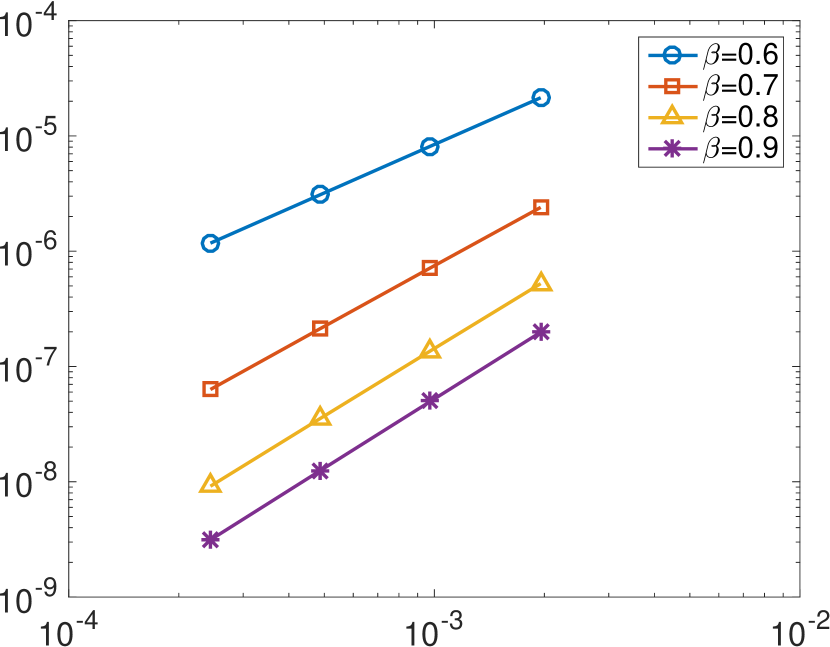
$f(u)=|u|^{2}$, $d=2$

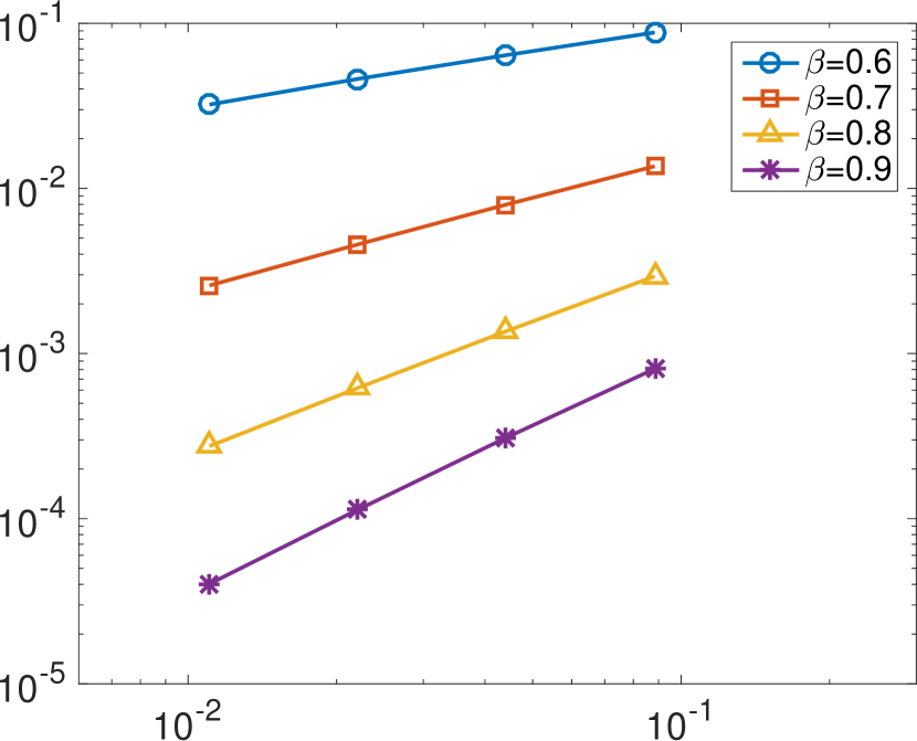
$f(u)=|u|^{3}$, $d=1$

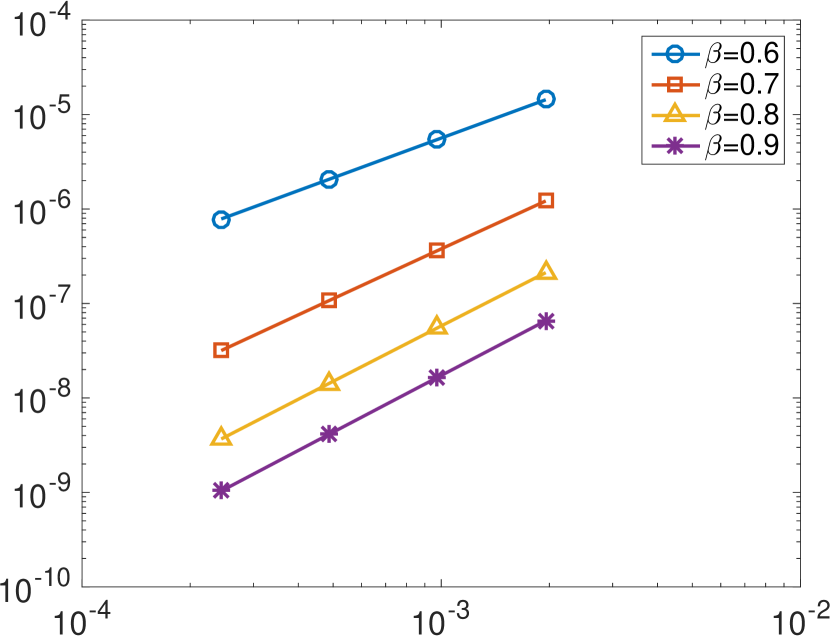
$f(u)=|u|^{3}$, $d=2$

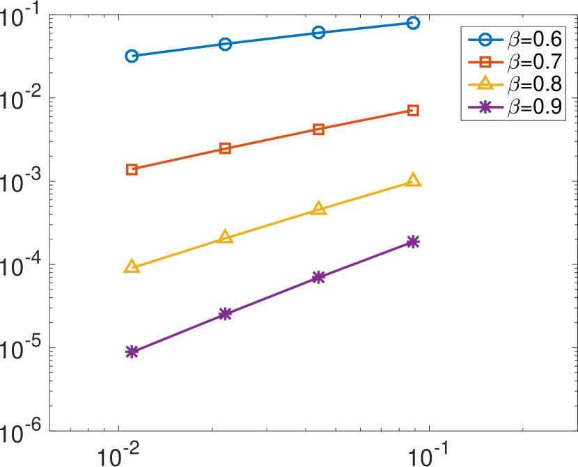
$f(u)=|u|^{4}$, $d=1$

$f(u)=|u|^{4}$, $d=2$

$f(u)=\Phi(20(u-0.5))$, $d=1$

$f(u)=\Phi(20(u-0.5))$, $d=2$

Figure 1. Observed weak errors for $d=1,2$ and different values of $\beta$. The errors for the four choices of $\varphi(u)=\int_{\mathcal{D}}f(u(\mathbf{x}))\,\mathrm{d}\mathbf{x}$ are shown as functions of the mesh size $h$ in a log-log scale. The corresponding observed convergence rates are shown in Table 2.

The resulting observed weak errors $\mathrm{err}_{\ell}:=|\mathbb{E}[\varphi(u)]-\mathbb{E}[\varphi(u_{h_{\ell},k}^{Q})]|$ are shown in Figure 1. For each function $\varphi$ and for each value of $\beta$, we compute the empirical convergence rate $\mathrm{r}$ by a least-squares fit of a line $\mathrm{c}+\mathrm{r}\ln h$ to the data set $\{h_{\ell},\mathrm{err}_{\ell}\}$. The results are shown in Table 2 and can be seen to validate the theoretical rates given in Theorem 2.4 for $d=1$. For $d=2$, the observed rates deviate slightly from the theoretical rates for $\beta=0.9$, which is caused by the fact that we had to use coarser finite element meshes for $d=2$ than for $d=1$ in order to be able to assemble the dense matrices $\mathbf{Q}_{h,k}^{\beta}\in\mathbb{R}^{N_{h}\times N_{h}}$ for performing the simulation study without Monte Carlo simulations.

Table 2. Observed (resp. theoretical) rates of convergence for the weak errors shown in Figure 1

		$\beta$
	$f(u)$	$0.6$	$0.7$	$0.8$	$0.9$
$d=1$	$|u|^{2}$	1.396 (1.4)	1.748 (1.8)	1.945 (2)	1.994 (2)
	$|u|^{3}$	1.397 (1.4)	1.753 (1.8)	1.949 (2)	1.995 (2)
	$|u|^{4}$	1.398 (1.4)	1.754 (1.8)	1.951 (2)	1.996 (2)
	$\Phi(20(u-0.5))$	1.398 (1.4)	1.755 (1.8)	1.952 (2)	1.996 (2)
$d=2$	$|u|^{2}$	0.483 (0.4)	0.800 (0.8)	1.139 (1.2)	1.442 (1.6)
	$|u|^{3}$	0.442 (0.4)	0.783 (0.8)	1.145 (1.2)	1.465 (1.6)
	$|u|^{4}$	0.409 (0.4)	0.768 (0.8)	1.143 (1.2)	1.472 (1.6)
	$\Phi(20(u-0.5))$	0.512 (0.4)	0.782 (0.8)	1.135 (1.2)	1.458 (1.6)

5. Conclusion

Gaussian random fields are of great importance as models in spatial statistics. A popular method for reducing the computational cost for operations, which are needed during statistical inference, is to represent the Gaussian field as a solution to an SPDE. In this work, we have investigated a recent extension of this approach to Gaussian random fields with general smoothness proposed in [4]. The method considers the fractional order equation (2.1) and is based on combining a finite element discretization in space with the quadrature approximation (2.4) of the inverse fractional power operator. This yields an approximate solution $u_{h,k}^{Q}$ of the SPDE, which in [4] was shown to converge to the solution $u$ of (2.1) in the strong mean-square sense with rate (2.7).

In many applications one is mostly interested in a certain quantity of the random field $u$ which can be expressed by $\varphi(u)$ for some real-valued function $\varphi$. For this reason, the focus of the present work has been the weak error $|\mathbb{E}[\varphi(u)]-\mathbb{E}[\varphi(u_{h,k}^{Q})]|$. The main outcome of this article, Theorem 2.4, shows convergence of this type of error to zero at an explicit rate for twice continuously Fréchet differentiable functions $\varphi$, which have a second derivative of polynomial growth. Notably, the component of the convergence rate stemming from the stochasticity of the problem is doubled compared to the strong convergence rate (2.7) derived in [4]. For proving this result, we have performed a rigorous error analysis in §3, which is based on an extension of the equation (2.1) to a time-dependent problem as well as an associated Kolmogorov backward equation and Itô calculus.

In order to validate the theoretical findings, we have performed a simulation study for the stochastic model problem (1.1) on the domain $\mathcal{D}=(0,1)^{d}$ for $d=1,2$ in §4. This model is highly relevant for applications in spatial statistics, since it is often used to approximate Gaussian Matérn fields. We have considered four different functions $\varphi$ and the fractional orders $\beta=0.6,0.7,0.8,0.9$. The observed empirical weak convergence rates can be seen to verify the theoretical results. One of the considered functions $\varphi$ is based on a transformation of the random field by a Gaussian cumulative distribution function. Quantities of this form are particularly important for applications to porous materials, as they are used to model the pore volume fraction of the material, see, e.g., [1]. Thus, we see ample possibilities for applying the outcomes of this work to problems in spatial statistics and related disciplines.

References

- [1] S. Barman and D. Bolin, A three-dimensional statistical model for imaged microstructures of porous polymer films, J. Microsc., 269 (2018), pp. 247–258.
- [2] D. Bolin, Spatial Matérn fields driven by non-Gaussian noise, Scand. J. Statist., 41 (2014), pp. 557–579.
- [3] D. Bolin and K. Kirchner, The rational SPDE approach for Gaussian random fields with general smoothness. arXiv preprint, arXiv:1711.04333v2, 2018.
- [4] D. Bolin, K. Kirchner, and M. Kovács, Numerical solution of fractional elliptic stochastic PDEs with spatial white noise. arXiv preprint, arXiv:1705.06565v2, 2018.
- [5] D. Bolin and F. Lindgren, Spatial models generated by nested stochastic partial differential equations, with an application to global ozone mapping, Ann. Appl. Statist., 5 (2011), pp. 523–550.
- [6] A. Bonito and J. E. Pasciak, Numerical approximation of fractional powers of elliptic operators, Math. Comp., 84 (2015), pp. 2083–2110.
- [7] Z. Brzeźniak, Some remarks on Itô and Stratonovich integration in 2-smooth Banach spaces, in Probabilistic methods in fluids, World Sci. Publ., River Edge, NJ, 2003, pp. 48–69.
- [8] R. Courant and D. Hilbert, Methods of Mathematical Physics: Vol. I, Interscience Publishers, Inc., New York, 1953.
- [9] G. Da Prato and J. Zabczyk, Second Order Partial Differential Equations in Hilbert Spaces, London Mathematical Society Lecture Note Series, Cambridge University Press, 2002.
- [10] G.-A. Fuglstad, F. Lindgren, D. Simpson, and H. Rue, Exploring a new class of non-stationary spatial Gaussian random fields with varying local anisotropy, Statistica Sinica, 25 (2015), pp. 115–133.
- [11] M. Kovács and J. Printems, Weak convergence of a fully discrete approximation of a linear stochastic evolution equation with a positive-type memory term, J. Math. Anal. Appl., 413 (2014), pp. 939 – 952.
- [12] F. Lindgren, H. Rue, and J. Lindström, An explicit link between Gaussian fields and Gaussian Markov random fields: the stochastic partial differential equation approach (with discussion), J. Roy. Statist. Soc. Ser. B Stat. Methodol., 73 (2011), pp. 423–498.
- [13] B. Matérn, Spatial variation, Meddelanden från statens skogsforskningsinstitut, 49 (1960).
- [14] A. Pazy, Semigroups of Linear Operators and Applications to Partial Differential Equations, Applied Mathematical Sciences, Springer, 1983.
- [15] S. Peszat and J. Zabczyk, Stochastic Partial Differential Equations with Lévy Noise, Encyclopedia of Mathematics and its Applications, Cambridge University Press, 2007.
- [16] H. Rue and L. Held, Gaussian Markov Random Fields: Theory and Applications, Chapman & Hall/CRC Monographs on Statistics & Applied Probability, CRC press, 2005.
- [17] M. L. Stein, Interpolation of Spatial Data: Some Theory for Kriging, Springer Series in Statistics, Springer New York, 1999.
- [18] G. Strang and G. Fix, An Analysis of the Finite Element Method, Wellesley-Cambridge Press, 2008.
- [19] V. Thomée, Galerkin Finite Element Methods for Parabolic Problems, Springer Series in Computational Mathematics, Springer Berlin Heidelberg, 2006.
- [20] J. Wallin and D. Bolin, Geostatistical modelling using non-Gaussian Matérn fields, Scand. J. Statist., 42 (2015), pp. 872–890.
- [21] P. Whittle, On stationary processes in the plane, Biometrika, 41 (1954), pp. 434–449.
- [22] , Stochastic processes in several dimensions, Bull. Internat. Statist. Inst., 40 (1963), pp. 974–994.