Observation of vortex-nucleated magnetization reversal in individual ferromagnetic nanotubes

Abstract

The reversal of a uniform axial magnetization in a ferromagnetic nanotube (FNT) has been predicted to nucleate and propagate through vortex domains forming at the ends. In dynamic cantilever magnetometry measurements of individual FNTs, we identify the entry of these vortices as a function of applied magnetic field and show that they mark the nucleation of magnetization reversal. We find that the entry field depends sensitively on the angle between the end surface of the FNT and the applied field. Micromagnetic simulations substantiate the experimental results and highlight the importance of the ends in determining the reversal process. The control over end vortex formation enabled by our findings is promising for the production of FNTs with tailored reversal properties.

The study of magnetization reversal in magnetic nanostructures is a topic of major fundamental and practical interest. In particular, a controllable, fast, and reproducible reversal is crucial for applications in high density magnetic storage. This process, however, is often conditioned by the presence of edge and surface domains. Near borders, magnetization tends to change direction in order to minimize stray field energy. As a result, the form of surfaces and edges – including any imperfections or roughness – determines the configuration of the magnetization in their vicinity. The resulting magnetization inhomogeneities tend to affect reversal by acting as nucleation sites for complex switching processes Coey (2010); Rothman et al. (2001). Furthermore, small differences in the initial configurations of edge and surface domains can lead to entirely different reversal modes, complicating the control and reproducibility of magnetic switching from nanomagnet to nanomagnet Zheng and Zhu (1997).

The high surface-to-volume ratio of magnetic nanostructures makes mitigating these effects essential in the design of high-density memory elements. One way to reduce the effect of edges and surfaces on magnetic reversal is to use magnetic structures that support flux-closure magnetization configurations Kent and Stein (2011). Since these configurations minimize stray field, edges and surfaces play a minor role in determining both their equilibrium state and their dynamics. Ferromagnetic nanotubes (FNTs) are one type of nanostructure supporting such states. In particular, reversal of uniform axial configurations in FNTs has been predicted to nucleate and propagate through vortex configurations, which appear at the FNT ends and whose magnetization curls around their hollow core Usov et al. (2007); Landeros et al. (2007, 2009); Landeros and Núñez (2010). Theory has so far only considered FNTs with perfect, flat ends, despite their importance as the nucleation sites of the reversal. Here, we show the experimental signatures of this nucleation and reveal its dependence on the angle of the FNT ends. Magnetization reversal in FNTs offers some potential advantages over the equivalent and well-understood process in ferromagnetic nanowires: in particular, the core-free geometry of FNTs has been predicted to favor uniform switching fields and high reproducibility Wang (2005); Escrig et al. (2007); Landeros et al. (2007). Understanding and controlling the switching process in real FNTs is a crucial step in enabling practical applications.

We study magnetization reversal in individual FNTs using dynamic cantilever magnetometry (DCM). This technique involves a measurement of the mechanical resonance frequency $f$ of a cantilever, to which the FNT of interest has been attached, as a function of a uniform externally applied magnetic field $\mathbf{H}$. The frequency shift $\Delta f=f-f_{0}$, where $f_{0}$ is the resonance frequency at $H=0$, reveals the curvature of the magnetic energy with respect to rotations about the cantilever oscillation axis Mehlin et al. (2015); Gross et al. (2016):

$$\Delta f=\frac{f_{0}}{2k_{0}l_{e}^{2}}\left(\left.\frac{\partial^{2}E_{m}}{\partial\theta_{c}^{2}}\right|_{\theta_{c}=0}\right),$$ (1)

where $k_{0}$ is the cantilever’s spring constant, $l_{e}$ its effective length, and $\theta_{c}$ its angle of oscillation. We simulate the DCM measurements by constructing a micromagnetic model of the experiment with the software package Mumax3 Vansteenkiste et al. (2014), which employs the Landau-Lifshitz-Gilbert micromagnetic formalism using finite-difference discretization. The simulations allow us to relate DCM signal to the magnetization configurations present in a FNT. These insights – combined with the high torque sensitivity provided by ultrasoft Si cantilevers – uncover magnetization reversal behavior of an individual FNT.

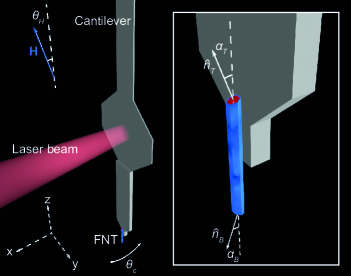
Figure 1: Schematic diagram of the measurement setup: Si cantilever (gray) and CoFeB FNT (blue) with GaAs core (red). The cantilever oscillates about $\hat{y}$ and the FNT axis is parallel to $\hat{z}$. The externally applied magnetic field $\mathbf{H}$ can be rotated in the $xz$-plane by an angle $\theta_{H}$ with respect to $\hat{z}$. The top (bottom) end of the FNT lies in a plane perpendicular to $\hat{n}_{T}$ ($\hat{n}_{B}$).

FNT samples consist of a 30-nm-thick ferromagnetic shell of CoFeB surrounding a non-magnetic GaAs core with hexagonal cross-section. The amorphous and homogeneous CoFeB shell is magnetron sputtered onto template GaAs nanowires, which are grown by molecular beam epitaxy Rüffer et al. (2014). Scanning electron micrographs (SEMs) of the studied FNTs reveal continuous and defect-free surfaces, whose roughness is less than 5 nm Sup . The FNTs have a diameter, which we define as the diameter of the circle circumscribing their hexagonal cross-section, between 270 and 300 nm. Lengths from 0.6 to 2.9 $\mathrm{\SIUnitSymbolMicro m}$ are obtained by cutting individual FNTs into segments using a focused ion beam (FIB) Wyss et al. (2017). This procedure ensures FNTs with smooth and well-defined ends, which – in general – are tilted relative to the plane normal to the FNT axis, as shown in Fig. 1. After cutting, each FNT is affixed to the end of an ultrasoft Si cantilever, which is mounted in the DCM measurement setup.

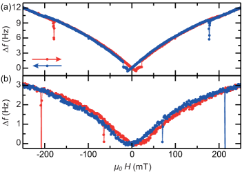
Figure 2: Magnetic reversal of (a) a 2.2-$\mathrm{\SIUnitSymbolMicro m}$-long and (b) a 0.6-$\mathrm{\SIUnitSymbolMicro m}$-long FNT measured by DCM at 280 K. $\mathbf{H}$ is applied approximately along $\hat{z}$. As in all following figures, color-coded arrows denote the direction that the magnetic field is stepped.

Fig. 2 shows DCM measurements at 280 K of two FNTs of different lengths: (a) 2.2 $\mathrm{\SIUnitSymbolMicro m}$ and (b) 0.6 $\mathrm{\SIUnitSymbolMicro m}$. For each FNT, measured $\Delta f(H)$ is plotted for $\mathbf{H}$ applied approximately along its long axis $\hat{z}$ and swept in the positive and negative direction. Since the cantilevers used here have similar mechanical properties, the magnitude of the frequency response is roughly proportional to the FNT length and therefore to the volume of magnetic material. Three major characteristics can be identified in the data sets. First, both show an overall V-shape, consistent with the near coincidence of the FNT easy axis and $\mathbf{H}$ Gross et al. (2016). Second, one or two spikes toward negative $\Delta f$ occur in forward applied field between $\pm 220$ and $\pm 60$ mT as well as weak echos of these features in reverse magnetic field. Third, around zero field, where the slope of $\Delta f(H)$ inverts, a distinct difference between the two FNTs is evident. The shorter FNT shows a parabolic dependence, without ever becoming negative, while the longer one crosses to negative values of $\Delta f$ before exhibiting two discontinuous steps. The latter behavior is similar to that found for an even longer 2.9-$\mathrm{\SIUnitSymbolMicro m}$-long FNT Sup . Measurements on FNTs of all three lengths were carried out at 4 K with similar results Sup .

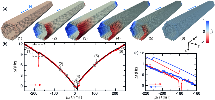
Figure 3: Simulated and measured reversal of a 2.2-$\mathrm{\SIUnitSymbolMicro m}$-long FNT. (a) Calculated magnetization configurations for $\Delta f(H)$ corresponding to the labels. (b) Simulated (lines) and measured (points) DCM signal. Squares highlight simulated vortex entry/exit features, which are difficult to see. (c) A detailed view of DCM signatures of vortex entrance and exit. For the simulation, $\alpha_{T}=6.5^{\circ}$, $\alpha_{B}=10.5^{\circ}$, and $\theta_{H}=11.0^{\circ}$.

The dimensions of a FNT are predicted to have a determining influence on its magnetic reversal. In particular, FNTs with a larger than critical diameter, reverse via nucleation of vortex rather than transverse domain walls Landeros et al. (2009); Landeros and Núñez (2010). Since this diameter ranges from a few nanometers to 20 nm, all experimentally fabricated FNTs should reverse through vortex domains. For long FNTs, i.e. 2 $\mathrm{\SIUnitSymbolMicro m}$ or longer for our cross-sectional geometry, the expected progression of the magnetization for $\mathbf{H}$ approximately along $\hat{z}$ can be summarized as shown in Fig. 3 (a). This specific progression is the result of our simulations, but similar progressions were predicted by previous analytical and numerical models Landeros et al. (2009); Gross et al. (2016). Starting from full saturation at negative $H$, vortices enter the two tube ends, setting the nucleation field of the reversal. At these fields, both relative circulation senses of the end domains have equal energy, such that the appearance of one or the other is likely driven by sample imperfections. As $H$ approaches zero and becomes positive, the vortices grow along the tube axis toward the center. At a small positive reverse field, the magnetization in the central axial domain irreversibly inverts, while the end vortices persist. From here on, the vortices shrink in size with progressively larger positive $H$, until they exit the FNT, marking the end of the reversal.

Fig. 3 (b) shows measured and simulated $\Delta f(H)$ for the 2.2-$\mathrm{\SIUnitSymbolMicro m}$-long FNT as $H$ is swept in the positive direction. The simulated $\Delta f(H)$ is calculated using the measured properties of the cantilever and the geometrical and material parameters of the FNT (adjusted within their error). Numerical labels indicate the magnetization configuration in Fig. 3 (a) corresponding to a particular value of $H$ in Fig. 3 (b). This correspondence allows us to attribute the discontinuous feature at $\mu_{0}H\approx-180$ mT in $\Delta f(H)$, between (1) and (2), to the entrance of the first end vortex. The entrance of the second vortex, marked by a square between (2) and (3), though not visible in the measurement, produces a tiny step in the simulated response at $\mu_{0}H\approx-40$ mT. Once at $H=0$, the FNT occupies configuration (3) with two end vortices and an axially aligned central domain. Between $\mu_{0}H\approx 10$ and 25 mT, an irreversible switching process causes the magnetization in the central domain to flip, forming configuration (4) and producing a change in the sign and slope of $\Delta f(H)$. The exit of the second vortex between (4) and (5) can then be attributed to the discontinuity at $\mu_{0}H\approx 100$ mT, while the first vortex exits between (5) and (6) producing the feature at $\mu_{0}H\approx 200$ mT.

In Fig. 3 (c) we highlight the entrance and exit of the first end vortex in both measured and simulated $\Delta f(H)$. The hysteresis marks the first and last irreversible processes of the magnetic reversal, indicating its nucleation and end, respectively. We find that both the magnitude in $\Delta f$ of the simulated vortex entry and exit features and the field, at which they occur, depend on the orientation of the FNT end surfaces (see $\hat{n}_{T}$ and $\hat{n}_{B}$ in inset to Fig. 1) with respect to $\mathbf{H}$. In the simulation, the angles of the ends with respect to the FNT long axis, $\alpha_{T}$ and $\alpha_{B}$, are carefully adjusted to match the measurements. For the 2.2-$\mathrm{\SIUnitSymbolMicro m}$-long FNT shown in Fig. 3 $\alpha_{T}\neq-\alpha_{B}$ ($\hat{n}_{T}\nparallel\hat{n}_{B}$), resulting in two distinct pairs of entrance and exit fields. One entrance and exit pair is barely visible in both experiment and simulation due to that end’s specific orientation with respect to $\mathbf{H}$ Sup . The strong negative spike in the measurements is not reproduced by the simulations. Although the origin of this feature is unclear, changes in $\Delta f$ toward more negative values correspond to a reduction in the angular magnetic confinement, indicating a disordered intermediate magnetic configuration. Simulations predicting DCM signatures of vortex entrance and exit in FNTs have been carried out before, however, no corresponding features were measured, likely due to the lack of well-defined ends, e.g. jagged ends or ends terminated by a growth-induced spherical shell Gross et al. (2016).

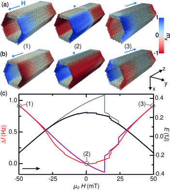
Figure 4: Simulated reversal of a 0.6-$\mathrm{\SIUnitSymbolMicro m}$-long FNT. Equilibrium magnetization configurations corresponding to the labeled points in $\Delta f(H)$ for a FNT initialized with vortex ends of (a) opposing and (b) matching circulation sense. (c) Plots of the simulated $\Delta f(H)$ in purple (red) and $E_{m}(H)$ in gray (black) for vortices of opposing (matching) circulation sense. For the simulation, $\alpha_{T}=6.0^{\circ}$, $\alpha_{B}=10.0^{\circ}$, and $\theta_{H}=10.0^{\circ}$.

Although the overall features of the measured and simulated $\Delta f(H)$ for the 2.2-$\mathrm{\SIUnitSymbolMicro m}$-long FNT match, there is a difference in the irreversible switching of the central domain (around $\mu_{0}H\approx\pm 20$ mT in Fig. 3 (b)). The measured response shows two distinct steps interrupted by a plateau-like feature, rather than the single step predicted by the simulations. Measurements at slightly different $\theta_{H}$ and of the 2.9-$\mathrm{\SIUnitSymbolMicro m}$-long FNT result in one to three such plateaus in the switching region Sup . These features indicate the presence of intermediate magnetization configurations near zero field Sup .

For short FNTs – FNTs less than 2-$\mathrm{\SIUnitSymbolMicro m}$-long for our cross-sectional dimensions – a different reversal process emerges. Since during reversal the two end vortices extend far enough to meet at the center of the FNT, the two relative circulation senses of the end domains lead to two different progressions, shown in Fig. 4 (a) and (b). For end domains of opposing circulation sense, simulations show that after the entrance of the vortices, the central axial domain shrinks until only a domain wall remains to separate the two vortex domains Chen et al. (2007, 2011). As $H$ becomes increasingly positive, the axial wall reverses in a series of irreversible steps, which are associated with the replacement of the axial wall in each facet with a Bloch or Neel-type vortex wall. After full reversal of the axial wall, the vortex domains recede, and exit.

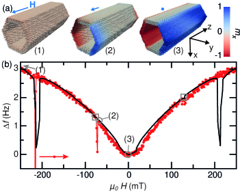
Figure 5: Simulated and measured reversal of a 0.6-$\mathrm{\SIUnitSymbolMicro m}$-long FNT. (a) Calculated magnetization configurations for $\Delta f(H)$ corresponding to the labels. (b) Simulated (lines) and measured (points) DCM response. Squares highlight simulated vortex entry/exit features, which are difficult to see. For the simulation, $\alpha_{T}=4.0^{\circ}$, $\alpha_{B}=6.5^{\circ}$, and $\theta_{H}=10.0^{\circ}$.

For end domains of matching circulation sense, simulations show a progression, in which the two vortex domains merge at the center of the FNT without forming a domain wall. In reverse field, this global vortex configuration progressively rotates toward $\mathbf{H}$, until it splits and the resulting end vortices exit as the FNT saturates. Steps occurring during this rotation are associated with the switching of the magnetization in each hexagonal edge, where two facets meet.

In Fig. 4 (c), we plot simulations of both $\Delta f(H)$ and the magnetic energy $E_{m}(H)$ associated with these two reversal progressions. Although end vortices with equal circulation represent the lower energy remanent configuration in short thin FNTs Chen et al. (2010); Wyss et al. (2017), both configurations have the same energy at high field within the accuracy of our simulation. Given the energy cost of switching between matching and opposing configurations, FNTs should – in principle – reverse via both reversal progressions. In fact, experiments on similar FNTs find both configurations in remanence after the application of an axial field Wyss et al. (2017), confirming the possibility of both reversal processes. Note that simulations plotted in Fig. 4 (c) predict distinct $\Delta f(H)$ signatures for short FNTs with end vortices of different relative circulation sense.

As shown in Fig. 5, the measured DCM response of the 0.6-$\mathrm{\SIUnitSymbolMicro m}$-long FNT matches the progression with vortices of matching circulation sense. $\Delta f(H)$ never drops below zero and is parabolic around zero field, indicating the presence of a remanent global vortex state. Features corresponding to the entrance and exit of the two end vortices match in field magnitude and to some extent also in $\Delta f$, with the exception of the large feature connected with the exit of the first vortex. This discrepancy is likely due to fine details of the end geometry not captured by our model.

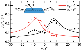
Figure 6: Simulated and measured dependence of vortex entrance field on field angle. Black (red) points show the measured $H_{en}$ as a function of $\theta_{H}$ for the top (bottom) end vortex in a single FNT. Black (red) solid lines show the corresponding simulations for $\alpha_{T}=6.0^{\circ}$ ($\alpha_{B}=6.0^{\circ}$). The schematic diagram depicts the FNT, its angled ends, and $\mathbf{H}$.

In all simulations, we tune the orientation of the plane in which the FNT ends lie ($\hat{n}_{T}$ and $\hat{n}_{B}$) with respect to $\mathbf{H}$ in order to reproduce the measured features in $\Delta f(H)$ associated with vortex entry and exit. We study this dependence in more detail by measuring DCM in the 0.6-$\mathrm{\SIUnitSymbolMicro m}$-long FNT as a function of $\theta_{H}$. Fig. 6 shows the experimentally determined and simulated entrance fields $H_{en}$ of the top (bottom) vortex domain in black (red) as a function of $\theta_{H}$. The corresponding exit fields, which are not shown, vary analogously. Measurements and simulations show that $H_{en}$ exhibits its absolute maximum just past $\theta_{H}=\pm\alpha_{T/B}$, i.e. $\mathbf{H}\parallel\hat{n}_{T/B}$. Upon a slight tilt of $\mathbf{H}$ away from this condition, $H_{en}$ is reduced. We attribute this behavior to the avoidance of magnetic surface charge density $\sigma$. In a saturated FNT, $\sigma$ at the ends is maximized for $\mathbf{H}\parallel\hat{n}_{T/B}$. As a consequence, this alignment also maximizes the reduction in magnetostatic energy resulting from the entrance of a vortex. At $H_{en}$, this reduction is equal to the corresponding Zeeman and exchange energy penalties. Given that the Zeeman penalty scales with field, a maximum in $H_{en}$ is expected for $\mathbf{H}\parallel\hat{n}_{T/B}$. The close agreement between experiment and simulation in Fig. 6 suggests that the simulated reversal nucleation process is an accurate description of the process occurring in the measured samples. Further simulations confirm that, for a fixed orientation of $\mathbf{H}$, $H_{en}$ – and therefore the reversal nucleation field – can be reduced from 250 to under 25 mT by increasing the the slant angle $\alpha_{T/B}$ from 0 to 30^∘ Sup .

In conclusion, we find that even slightly slanted ends considerably shift the nucleation field for axial magnetization reversal in FNTs. Still, the magnetization reversal process is observed to occur through vortex configurations, as originally predicted. This experimental confirmation of vortex-nucleated reversal and the demonstrated tunability of the vortex entry field set the stage for the realization of FNTs with fast and highly reproducible switching behavior.

Appendix A Ferromagnetic Nanotube Fabrication

The template nanowires (NWs), onto which the CoFeB shell forming the ferromagnetic nanotubes (FNTs) is sputtered, are grown by molecular beam epitaxy on a Si (111) substrate using Ga droplets as catalysts Rüffer et al. (2014). During CoFeB deposition, a wafer of upright and well-separated GaAs NWs is mounted with a 35^∘ angle between the long axis of the NWs and the deposition direction. The wafer is then continuously rotated in order to achieve a conformal coating. We cut individual FNTs into segments of different lengths and with well-defined ends using a focused ion beam (FIB). After cutting, we use an optical microscope equipped with precision micro-manipulators to pick up each FNT segment and affix it to the end of an ultrasoft Si cantilever. Non-magnetic epoxy (Gatan G1) is used as an adhesive.

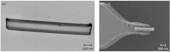
Figure 7: Scanning electron micrographs (SEMs) of the FIB milled 2.2 $\mu$m-long FNT (a) placed on a Si-surface and (b) attached to the tip of a ultra-soft Si cantilever.

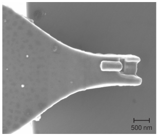
Figure 8: SEMs of the 0.6-$\mu$m-long FNT attached to the tip of a Si-cantilever. The FNT was shortened in a second FIB step after the FNT was already attached to the cantilever.

Appendix B Dynamic Cantilever Magnetometry

The dynamic cantilever magnetometry (DCM) measurement setup consists of a vibration-isolated vacuum chamber with a pressure below $10^{-4}$ mbar. A separate manually rotatable superconducting magnet allows the application of an external magnetic field $\mathbf{H}$ up to 4 T in any direction in the $xz$-plane. We use cantilevers made of undoped single-crystal Si with a length of 150 $\mu$m, width of 4 $\mu$m, and thickness of 0.1 $\mu$m. The spring constant $k_{0}=90$ $\mu$N/m and the effective length of the fundamental mode $l_{e}=105$ $\mu$m. Unlike the others, the cantilever used with the 2.2 $\mu$m-long FNT is 180 $\mu$m long, $k_{0}=70$ $\mu$N/m and $l_{e}=130$ $\mu$m. Deflection of the cantilever along $\hat{x}$ is measured using a fiber interferometer Rugar (1989) with 100 nW of 1550 nm laser light focused onto a 10-$\mu$m-wide paddle near the end of the cantilever. A piezo-electric actuator mechanically drives the cantilever at its resonance frequency with a constant oscillation amplitude of 40 nm using a feed-back loop implemented by a field-programmable gate array. This process of self-oscillation enables the fast and accurate extraction of the resonance frequency $f$ from the cantilever deflection signal. Before measurement, we stabilize the temperature and fully magnetize the sample at large $\mathbf{H}$. DCM data is then collected as the field is stepped toward zero and into reverse field.

Appendix C Mumax3 Simulations

We set $\mu_{0}M_{S}$ to its measured value of $1.3\text{\,}\mathrm{T}$ Gross et al. (2016) and the exchange stiffness to $A_{ex}=$28\text{\,}\mathrm{pJ}$/$\mathrm{m}$$. We model the FNTs as perfectly hexagonal tubes with slanted ends. Discretization of space with cubic mesh elements leads to a staircase effect on all slanted surfaces, which could have a impact on the magnetic states that are calculated to be stable. In order to exclude spurious results due to such simulation artifacts, we perform reference simulations with the finite element package nmag Fischbacher et al. (2007), which avoids staircase effects by using irregular tetragonal meshes. In particular, nmag simulations reveal the same stable magnetization configurations, the same vortex entry mechanism, and the same values for the vortex entry (exit) field $H_{en}$ ($H_{ex}$). As a result, we conclude that the staircase effect on the FNT ends does not have a significant effect on our simulation results.

Both Mumax3 and nmag are used to determine the equilibrium magnetization configuration for each external field value by numerically solving the Landau-Lifshitz-Gilbert equation. Since the microscopic processes in FNTs are expected to be much faster than the cantilever resonance frequency Landeros and Núñez (2010); Schwarze and Grundler (2013); Yan et al. (2012); Gross et al. (2016), the magnetization of the nanotube can always be assumed to be in its equilibrium orientation. The calculation also yields the total magnetic energy $E_{m}$ corresponding to each configuration. In order to simulate $\Delta f$ measured in DCM, we numerically calculate the second derivative of $E_{m}$ with respect to $\theta_{c}$ found in (1) in the main text. At each field, we calculate $E_{m}$ at the cantilever equilibrium angle $\theta_{c}=0$ and at small deviations from equilibrium $\theta_{c}=\pm\delta\theta_{c}$. For small $\delta\theta_{c}$, the second derivative can by approximated by a finite difference: $\left.\frac{\partial^{2}E_{m}}{\partial\theta_{c}^{2}}\right|_{\theta_{c}=0}\approx\frac{E_{m}(\delta\theta_{c})-2E_{m}(0)+E_{m}(-\delta\theta_{c})}{(\delta\theta_{c})^{2}}$. By setting $f_{0}$, $k_{0}$, and $l_{e}$ to their measured values, we then arrive at the $\Delta f$ corresponding to each magnetization configuration in the numerically calculated field dependence. Table 1 shows the exact parameters for the geometry of the FNT and the direction of the applied field used for the simulations shown in the main text.

Table 1: Parameters used for the simulations shown in the main text. $d$ is the FNT diameter, $t$ its thickness, $l$ its length, $\alpha_{T}$ ($\alpha_{B}$) the slant angle of its top (bottom) end, $\theta_{H}$ ($\phi_{H}$) is the polar (azimuthal) angle of $\mathbf{H}$, $\delta\theta_{c}$ is the cantilever deviation angle used to calculate $\Delta f$, and $\epsilon_{m}$ is the mesh size.

Fig.	$d$ (nm)	$t$ (nm)	$l$ ($\mu$m)	$\alpha_{T}$ (∘)	$\alpha_{B}$ (∘)	$\theta_{H}$ (∘)	$\phi_{H}$ (∘)	$\delta\theta_{c}$ (∘)	$\epsilon_{m}$ (nm)
3	280	30	2.180	6.5	10.5	11.0	-6.0	2.0	5
4	284	30	0.640	6.0	10.0	10.0	1.0	1.0	4
5	284	30	0.640	4.0	6.5	10.0	1.0	1.0	4
6	284	30	0.640	6.0	6.0	-	1.0	1.0	4

Appendix D Reversal Measured at Low Temperature

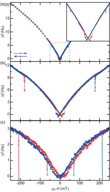
Figure 9: Magnetic reversal of the three FNTs of different lengths measured by DCM at 280 K: (a) the 2.9-$\mu$m-long, including a zoom of the low field region; (b) the 2.2-$\mu$m-long; and (c) the 0.6-$\mu$m-long FNT.

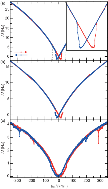
Figure 10: Magnetic reversal of the three FNTs of different lengths measured by DCM at 4 K: (a) the 2.9-$\mu$m-long, including a zoom of the low field region; (b) the 2.2-$\mu$m-long; and (c) the 0.6-$\mu$m-long FNT.

Fig. 9 shows DCM measurements at 280 K of three FNTs of different lengths. Measurements of a 2.9-$\mu$m-long FNT are shown in (a), while measurements of a 2.2-$\mu$m-long FNT and 0.6-$\mu$m-long FNT, which already appear in the main text, are shown in (b) and (c), respectively. As expected from numerical simulations and theory, the FNTs longer than 2 $\mu$m display a qualitatively similar behavior corresponding to a common magnetization reversal process.

Fig. 10 shows a second set of DCM measurements of the same three FNTs carried out at 4 K. Although the same qualitative features observed at 280 K can be recognized, various details of the reversal differ. First, the features in $\Delta f(H)$ indicating the entrance or exit of a vortex are less pronounced at low temperature than at 280 K (shown in Fig. 2). Second, for the two longer FNTs, the hysteric region marking an irreversible switching process spans a larger field range at low temperature than at high temperature. This behavior reflects the smaller amount of thermal energy available to the system at low temperature to overcome the energy barriers impeding magnetization reversal. Although the entrance and exit of the two vortices appear at similar fields for all FNTs at both 4 K and 280 K, differences in the angle of the magnetic field $\theta_{H}$ for each measurement preclude drawing conclusions about the dependence of entrance/exit field on temperature.

Appendix E Plateau in $\Delta f$ for small applied fields

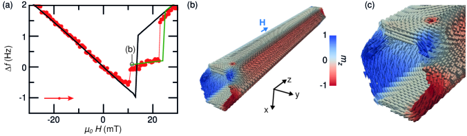
Figure 11: (a) A detailed view of the simulated (line) and measured (points) DCM signatures of the irreversible switching at low-field for the 2.2-$\mu$m-long FNT. The green line shows the DCM response of a magnetization configuration, shown in (b) and (c), which is initialized and calculated to be stable at $H=0$. The configuration includes two vortices each residing in a hexagonal facet of the FNT and produces a $\Delta f(H)$, which matches the plateau appearing in the measured response.

DCM measurements shown in Fig. 2 (a) and Fig. 10 (a) and (b) show plateau-like features in the irreversible switching region around zero field that are not predicted by the simulations. The behavior in $\Delta f(H)$ can be reproduced, however, by initializing the FNT configuration at $H=0$. For example, by initializing the FNT with two vortices each residing in a hexagonal facet of the FNT and sweeping $H$ from zero to positive fields, a plateau in the simulated $\Delta f(H)$ emerges, as shown in Fig. 11 (a). This plateau feature corresponds to an intermediate configuration with two facet vortices, shown in Fig. 11 (b) and (c). Following the irreversible switch around 25 mT, these facet vortices ’rotate’ around $\hat{y}$ and take their place as the end vortices of an FNT in a mixed state configuration. In this picture, the irreversible switching of the FNTs central axial domain is characterized by the ’rotation’ of end vortices into the facets – consuming the axial domain and resulting in the plateau in $\Delta f(H)$ – followed by a second rotation of the vortices from the facets back to the ends. Similar states are present in the simulations for short FNTs with opposing vortex circulation sense. For example, the plateau between 12 and 25 mT in the purple $\Delta f(H)$-curve in Fig. 4 (c) is the result of a configuration with two facet vortices. Although this reversal mode is a possibility which matches the measured $\Delta f(H)$ near zero field, we cannot rule out the possibility of other intermediate configurations resulting in the same DCM response.

Appendix F Simulated and Measured Vortex Entrance

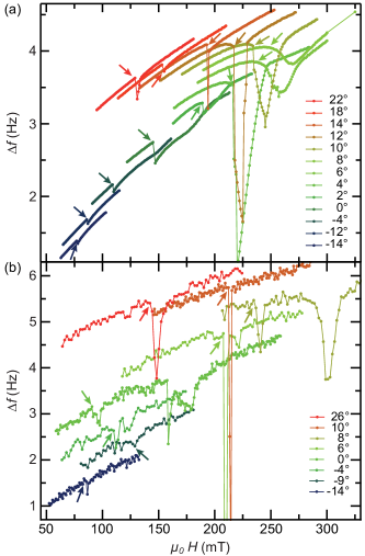
Figure 12: (a) simulated and (b) measured segments of $\Delta f(H)$ showing the vortex formation in a 0.6 $\mu$m-long NT for different values of $\theta_{H}$ as labeled in the plots. Arrows highlight the specific feature corresponding to the vortex entrance, as indicated in corresponding simulations of the FNT magnetization configuration.

Fig. 6 of the main text illustrates the dependence of the vortex entrance on the magnetic field angle $\theta_{H}$. The data plotted in that figure are extracted from the DCM measurements shown in Fig. 12. This figure shows a comparison between (a) simulated and (b) measured $\Delta f(H)$ in the region of one vortex entrance for the 0.6-$\mu$m-long FNT. Note the strong dependence of the magnitude in $\Delta f$ of the entrance features on $\theta_{H}$. As with the value of $H_{en}$, this magnitude is maximized for $\mathbf{H}\parallel\hat{n}_{T/B}$. In other words, the vortex entrance and exit features for an end whose normal is strongly misaligned with $\mathbf{H}$ are nearly invisible by DCM.

Appendix G Control of Reversal Nucleation Field

Fig. 6 makes clear that the angle of the applied magnetic field $\theta_{H}$ affects the entrance field of the vortex and thus the reversal nucleation field of the FNT. Fig. 13 shows the simulated dependence of the entrance of the top vortex on the slant angle of the top FNT end $\alpha_{T}$ for a fixed $\theta_{H}$. The entrance field can be tuned by over 225 mT by changing the slant angle by $30^{\circ}$. These simulations, combined with the experimental evidence shown in the main text, show that reversal nucleation in FNTs can be finely and predictably controlled by tuning the geometry of their ends.

Figure 13: Simulated dependence of the entrance field $H_{en}$ of the top vortex on the slant angle of the top end $\alpha_{T}$ for the 0.6-$\mu$m-long FNT. The magnetic field is applied parallel to $\hat{z}$, i.e. $\theta_{H}=0$.

Appendix H Simulation of Vortex Entrance

The supplementary animation VortexEntrance shows the progression of magnetization configurations present in the 0.6-$\mu$m-long FNT as the magnetic field is reduced from positive values towards zero. At the same time, the animation shows the simulated values of $\Delta f(H)$, making clear the correspondence between a discontinuous feature in $\Delta f(H)$ – similar to those observed in our measurements – and the vortex entrance. In this particular simulation, the field is applied with an angle $\theta_{H}=14^{\circ}$ with respect to the long axis of the FNT.

References

- Coey (2010) J. M. D. Coey, Magnetism and Magnetic Materials (Cambridge University Press, 2010).
- Rothman et al. (2001) J. Rothman, M. Kläui, L. Lopez-Diaz, C. A. F. Vaz, A. Bleloch, J. A. C. Bland, Z. Cui, and R. Speaks, Phys. Rev. Lett. 86, 1098 (2001).
- Zheng and Zhu (1997) Y. Zheng and J.-G. Zhu, J. Appl. Phys. 81, 5471 (1997).
- Kent and Stein (2011) A. D. Kent and D. L. Stein, IEEE Trans. Nanotechnol. 10, 129 (2011).
- Usov et al. (2007) N. A. Usov, A. Zhukov, and J. Gonzalez, J. Magn. Magn. Mater. 316, 255 (2007).
- Landeros et al. (2007) P. Landeros, S. Allende, J. Escrig, E. Salcedo, D. Altbir, and E. E. Vogel, Appl. Phys. Lett. 90, 102501 (2007).
- Landeros et al. (2009) P. Landeros, O. J. Suarez, A. Cuchillo, and P. Vargas, Phys. Rev. B 79, 024404 (2009).
- Landeros and Núñez (2010) P. Landeros and A. S. Núñez, J. Appl. Phys. 108, 033917 (2010).
- Wang (2005) Z. Wang, Phys. Rev. Lett. 94 (2005).
- Escrig et al. (2007) J. Escrig, P. Landeros, D. Altbir, E. E. Vogel, and P. Vargas, J. Magn. Magn. Mater. 308, 233 (2007).
- Mehlin et al. (2015) A. Mehlin, F. Xue, D. Liang, H. F. Du, M. J. Stolt, S. Jin, M. L. Tian, and M. Poggio, Nano Lett. 15, 4839 (2015).
- Gross et al. (2016) B. Gross, D. P. Weber, D. Rüffer, A. Buchter, F. Heimbach, A. Fontcuberta i Morral, D. Grundler, and M. Poggio, Phys. Rev. B 93, 064409 (2016).
- Vansteenkiste et al. (2014) A. Vansteenkiste, J. Leliaert, M. Dvornik, M. Helsen, F. Garcia-Sanchez, and B. Van Waeyenberge, AIP Adv. 4, 107133 (2014).
- Rüffer et al. (2014) D. Rüffer, M. Slot, R. Huber, T. Schwarze, F. Heimbach, G. Tütüncüoglu, F. Matteini, E. Russo-Averchi, A. Kovács, R. Dunin-Borkowski, R. R. Zamani, J. R. Morante, J. Arbiol, A. Fontcuberta i Morral, and D. Grundler, APL Mater. 2, 076112 (2014).
- (15) See supplemental material .
- Wyss et al. (2017) M. Wyss, A. Mehlin, B. Gross, A. Buchter, A. Farhan, M. Buzzi, A. Kleibert, G. Tütüncüoglu, F. Heimbach, A. Fontcuberta i Morral, D. Grundler, and M. Poggio, Phys. Rev. B 96, 024423 (2017).
- Chen et al. (2007) A. P. Chen, N. A. Usov, J. M. Blanco, and J. Gonzalez, J. Magn. Magn. Mater. 316, e317 (2007).
- Chen et al. (2011) A.-P. Chen, J. M. Gonzalez, and K. Y. Guslienko, J. Appl. Phys. 109, 073923 (2011).
- Chen et al. (2010) A. P. Chen, K. Y. Guslienko, and J. Gonzalez, J. Appl. Phys. 108, 083920 (2010).
- Kläui et al. (2001) M. Kläui, J. Rothman, L. Lopez-Diaz, C. A. F. Vaz, and J. A. C. Bland, Appl. Phys. Lett. 78, 3268 (2001).
- Han et al. (2008) X. F. Han, Z. C. Wen, and H. X. Wei, J. Appl. Phys. 103, 07E933 (2008).
- Rugar (1989) D. Rugar, H. J.. Mamin, and P. Guethner, Appl. Phys. Lett. 55, 2588 (1989).
- Fischbacher et al. (2007) T. Fischbacher, M. Franchin, G. Bordignon, and H. Fangohr, IEEE Trans. Magn. 43, 2896 (2007).
- Schwarze and Grundler (2013) T. Schwarze and D. Grundler, Appl. Phys. Lett. 102, 222412 (2013).
- Yan et al. (2012) M. Yan, C. Andreas, A. Kákay, F. García-Sánchez, and R. Hertel, Appl. Phys. Lett. 100, 252401 (2012).