The Argyris isogeometric space on unstructured multi-patch planar domains
Abstract
Multi-patch spline parametrizations are used in geometric design and isogeometric analysis to represent complex domains. We deal with a particular class of planar multi-patch spline parametrizations called analysis-suitable (AS-) multi-patch parametrizations (cf. [10]). This class of parametrizations has to satisfy specific geometric continuity constraints, and is of importance since it allows to construct, on the multi-patch domain, isogeometric spaces with optimal approximation properties. It was demonstrated in [22] that AS- multi-patch parametrizations are suitable for modeling complex planar multi-patch domains.
In this work, we construct a basis, and an associated dual basis, for a specific isogeometric spline space over a given AS- multi-patch parametrization. We call the space the Argyris isogeometric space, since it is across interfaces and at all vertices and generalizes the idea of Argyris finite elements (see [1]) to tensor-product splines. The considered space is a subspace of the entire isogeometric space , which maintains the reproduction properties of traces and normal derivatives along the interfaces. Moreover, it reproduces all derivatives up to second order at the vertices. In contrast to , the dimension of does not depend on the domain parametrization, and admits a basis and dual basis which possess a simple explicit representation and local support.
We conclude the paper with some numerical experiments, which exhibit the optimal approximation order of the Argyris isogeometric space and demonstrate the applicability of our approach for isogeometric analysis.
keywords:
Isogeometric Analysis , Argyris isogeometric space , analysis-suitable parametrization , planar multi-patch domain1 Introduction
Multi-patch spline parametrizations are a powerful tool in computer-aided geometric design for modeling complex domains (cf. [13, 17]). In the framework of isogeometric analysis (IGA) (cf. [4, 11, 18]) the underlying spline spaces of these parametrizations are used to define (smooth) discretization spaces for numerically solving partial differential equations (PDEs) over the multi-patch domains. When solving a fourth order PDE, such as the biharmonic equation, e.g. [3, 10, 20, 23, 35], the Kirchhoff-Love plate/shell problem, e.g. [2, 5, 25, 26, 27], or the Cahn-Hilliard equation, e.g. [14, 15, 30], by means of its weak formulation using a standard Galerkin projection, approximating functions of global -smoothness are needed.
In this work we construct an isogeometric space with global regularity over an unstructured multi-patch parametrization. Our construction takes inspiration from the Argyris finite element [1], which has been the progenitor of all the triangular finite elements. The original Argyris construction uses polynomials of total degree and the following degrees-of-freedom: The function values, first and second derivatives at the element vertices, and the normal derivatives at the element edge midpoints. These degrees-of-freedom determine the trace at the edges (a polynomial of degree on each edge) and the normal derivatives at the edges (a polynomial of degree ), and by that, determine the polynomial on the whole triangle (see Figure 1(a)). regularity follows from the gluing of the normal derivative at the edges.
After Argyris, other constructions on triangular meshes have been proposed, in the context of finite elements (see for example the book [9]). The Argyris triangular element has been used only recently for surface parametrizations, in [19]. However, splines on triangular meshes are commonly used in geometric design, often with smoothness at the mesh vertices, see the book [29] for references.
In the finite element literature, the results on quadrilateral elements are restricted to meshes of structured rectangles, where the first and most well-known construction is the Bogner-Fox-Schmit element, introduced in [8]. Isogeometric analysis has been reinvigorating this interest: The recent papers [10, 20, 21, 23] and the book [6] shed light on the conditions of global regularity for isogeometric spaces on unstructured quadrilateral meshes, showing at the same time that these spaces are difficult to characterize. This motivates our present work: We design a basis and the related degrees-of-freedom for a subspace of the complete isogeometric space, mimicking the Argyris construction. The space we propose is therefore named Argyris isogeometric space and denoted by .
Consider a quadrilateral element , i.e., given by a bilinear mapping of the reference square element. The lowest-degree polynomial version of contains functions such that is a (bi)quintic polynomial, and is a quartic polynomial on the edges of the reference element. There are two main differences with respect to the original Argyris triangle. The first is obvious: is not polynomial since is not linear, in general. The second is technical: is not the normal unitary vector to the edges of , it is instead a suitable non-constant direction, shared with the adjacent quadrilateral and dependent on it. The degrees-of-freedom are indeed:
-
1.
(vertex) degrees-of-freedom giving the value, first and second derivatives at each vertex, fully determining the trace of at the boundary of the element,
-
2.
(edge) degrees-of-freedom, one per edge, that with the previous information fully determine as a quartic polynomial on each edge,
-
3.
(interior) degrees-of-freedom that, with the trace and directional derivative given at the boundary, fully determine .
The total number of degrees-of-freedom is and they are depicted in Figure 1(c). However the condition that is a quartic polynomial on each edge is responsible for additional scalar constraints due to degree elevation to quintic polynomials. The degrees-of-freedom together with the constraints give conditions, which matches the dimension of the (bi)quintic polynomial space. We remark that the boundary degrees-of-freedom above correspond to the ones of the original Argyris triangular element, with replacing (as for the Argyris triangular element, these edge degrees-of-freedom depend on the mesh and do not admit a universal definition on the reference element). Interior degrees-of-freedom appear also in the higher-degree Argyris triangular element, see Figure 1(b). Our construction is generalizable to any degree , see Figure 1(d).
The construction above further extends in two ways. The first is that, instead of a quadrilateral element, we can allow a Bézier patch, that is can be a -degree polynomial. However there are compatibility conditions between adjacent patch parametrizations that guarantee that the Argyris isogeometric space does not get overconstrained: We need the to form an analysis-suitable multi-patch parametrization (see [10]). The second extension is from a polynomial space (on each patch) to a tensor-product spline space. Not only is this important in isogeometric analysis, it also allows a degree reduction. Indeed we can construct an Argyris isogeometric patch from (bi)cubic continuous splines, see Figure 1(e).
In this paper we show that the Argyris isogeometric space is well defined by constructing a suitable basis and dual basis possessing desirable properties, such as local support and an explicit representation, which can be evaluated and manipulated easily.
A key ingredient of our approach is the determination of the compatibility conditions that the parametrizations of the patches need to fulfill in order to guarantee that the Argyris isogeometric space possesses optimal approximation order. This is based on the mentioned work [10], where the class of AS- multi-patch parametrizations has been introduced. The paper [22] has then shown numerically that this class of parametrizations enables the geometric design of complex planar multi-patch domains. The construction can be extended to surfaces, and the isogeometric spaces constructed on AS- multi-patch parametrizations exhibit optimal convergence under -refinement.
Piecewise bilinear multi-patch parametrizations are a subclass of the class of AS- multi-patch parametrizations and were considered to generate a basis in [6, 20, 23]. The focus therein is however to characterize the full isogeometric space, which we denote in this paper. The papers [20, 23] study for uniform spline functions of degree . The work [6] focuses on Bézier polynomials of degree and and generates basis functions by means of minimal determining sets (cf. [28]) for the involved Bézier coefficients. These approaches can be extended to mapped piecewise bilinear multi-patch parametrizations, which are also AS- and allow to model certain domains with curved boundaries and interfaces, see [20, 23]. Still, more general AS- multi-patch parametrizations, such as domains with smooth boundaries, cannot be handled. In [21] an explicit basis construction was given allowing non-uniform isogeometric spline functions of arbitrary degree and regularity (with regularity up to ), but on a two-patch geometry, with AS- parametrization.
Unlike the Argyris isogeometric space , the dimension of the full space, that is , depends on the domain parametrization, see [21]. In fact possesses a simpler structure than , but maintains its reproduction properties for traces and normal derivatives along the interfaces. In the present work we only provide numerical evidence of the optimal approximation properties of , postponing the mathematical analysis to a further work.
In our setting, and in the papers [6, 7, 10, 20, 21, 23, 31], the isogeometric functions are defined over a domain given by a multi-patch parametrization which is not at the patch interfaces. However there is another possibility, that is, when the multi-patch parametrization is everywhere except in the vicinity of an extraordinary vertex, where the parametrization is singular. isogeometric spaces in this case are constructed and studied in [24, 32, 33, 34, 39, 40, 41]. A special case is when the parametrization is polar at the extraordinary vertex, see [36, 37, 38].
The remainder of the paper is organized as follows. Section 2 presents some basic definitions and notations which are used throughout the paper. This includes the presentation of the spline spaces and of the multi-patch domain parametrizations as well as the local and global indexing for the patches, edges and vertices that we use. In Section 3 we recall the concept of AS- multi-patch parametrizations and the framework of isogeometric spline spaces over this class of multi-patch parametrizations. Section 4 describes the construction of a basis and of its associated dual basis for the Argyris isogeometric space . In Section 5 we perform -approximation over different AS- parametrizations to demonstrate the potential of the Argyris isogeometric space for applications in IGA. After the concluding remarks in Section 6, we deliver technical proofs in A, and describe in B and C some extensions of our construction.
2 Preliminaries
We describe the general notation as well as the multi-patch framework, which will be considered and used throughout the paper. First, in Sections 2.1 and 2.2 we introduce the general notation, the uni- and bivariate B-spline spaces and bases as well as the multi-patch domain we consider. Then, we recall in Section 2.3 the standard global-to-local index mapping of mesh objects within our framework. Finally, we introduce in Section 2.4 a specific local reparametrization, which will simplify the definitions of the smooth basis functions in Section 4.
2.1 Basic notation and spline spaces
We consider an open domain , connected and regular, and being its boundary. If is a manifold of dimension (a point) or (a line), we denote by the set of piecewise smooth functions defined on for which the -order derivatives are continuous at each point of .
We denote by the spline space of degree and continuity on the parameter domain , constructed from an open knot vector with non-empty knot-spans (i.e., elements), then having mesh size . We restrict here to uniform knot spans for simplicity, see [21] and B for the generalization. The multiplicity of the interior knots is .
Definition 1 (Univariate B-spline basis).
Given a integers , , and , we denote by , with , the standard B-spline basis for the univariate -degree polynomial space on with uniform mesh of mesh size .
The tensor-product spline space on the parameter (reference) domain is , where and indicate double indices which we assume, for the sake of simplicity, to be the same in the the two directions.
Remark 1.
For any , is the space of polynomials of degree .
Definition 2 (Tensor-product B-spline basis).
We denote the standard tensor-product B-spline basis of the space by , with , where and .
Assumption 3 (Minimum regularity within the patches).
We assume , that is, .
2.2 Multi-patch domain parametrization
We consider a multi-patch domain parametrization, composed of four-sided subdomains, called patches, interfaces between those patches as well as vertices, where several interfaces meet. The index sets containing all patches, all edges and all vertices will be denoted by , and , respectively. Moreover, we will have , where collects all indices representing the patch interfaces and the indices in represent all boundary edges. Similarly, we will have , where the indices in represent all interior vertices and the ones in represent all boundary vertices. To avoid confusion, we will denote all index sets of patches, interfaces and vertices with a calligraphic , and all index sets of basis functions with a double struck .
Assumption 4 (Multi-patch domain ).
The domain is the image of a regular multi-patch spline parametrization, i.e.,
| (1) |
where is a regular and disjoint partition, without hanging nodes, and each is an open spline patch,
| (2) |
where are non-singular and orientation-preserving, i.e., for all and for all , it holds
| (3) |
The domain is partitioned into the union of patches, interfaces and interior vertices
The boundary of the domain is given by the collection of boundary edges and boundary vertices
2.3 Global to local index conversion for edges and vertices
Each edge and vertex of the multi-patch partition corresponds to a global index or , respectively. In order to relate the edges and vertices to the patch parametrizations, each global index will be associated with a set of local indices, depending on the patches that share the edge or vertex.
The local index, which we define in the following, is in fact a multi-index , comprised of a patch index and a local numbering .
Remark 2.
We always denote with or dependent (secondary) indices, which depend on a (primary) index , e.g. , being the patches sharing an interface .
The four edges of each patch are indexed as follows:
| (4) |
for its four vertices we set:
see Figure 2. Here and in what follows, the local coordinate system is depicted with green and blue arrows, corresponding to the - and -parameter directions, respectively.
The global to local index conversion for the edges is defined as follows.
Assumption 5 (Global to local index conversion for edges).
For each global index there exists a set , with , , and , and
| (5) |
For each global index we have , with and , and
| (6) |
Similarly, we can define the global to local index conversion for vertices.
Assumption 6 (Global to local index conversion for vertices).
For each there exists a set , with , being different patch indices, and , where
| (7) |
Here, is the patch valence of the vertex .
Note that we only consider even sub-indices for all patches. This is because later we introduce odd sub-indices for the adjacent interfaces (see Figure 3 and Definition 8). The patch valence coincides with the edge valence for interior vertices (this is the classical notion of valence). For boundary vertices the edge valence is larger by one than the patch valence.
Note that the inverse mapping from local to global indices is unique in the following sense: Each local edge index is associated to a unique global index of an interface or a boundary edge, i.e., for each and for each there exists exactly one , such that . Moreover, for each and for each there exists exactly one , such that .
2.4 Parametrization in standard form for edges and vertices
In order to simplify the construction of smooth basis functions across interfaces and vertices, we assume that the patch parametrizations are given in standard form, as depicted in Figure 3. This is obviously not always the case, but can be achieved by reparametrization, as we will demonstrate in Lemma 1.
For an interface in standard form, we assume that the two neighboring patches meet in a certain way, as given in the following definition.
Definition 7.
Given an interface , for , and let , be the corresponding patch indices as in Assumption 5. We have given a parametrization in standard form for the interface , if
| (8) |
This corresponds to a configuration as depicted in Figure 3 (left). Similarly, for a boundary edge , with , we say that a parametrization in standard form is given if .
For a vertex in standard form, we assume that the vertex is enclosed by edges and patches
in counterclockwise order and that the patches are parametrized in such a way that the vertex is at the origin, as depicted in Figure 3 (right). This is detailed in the following definition.
Definition 8.
Given a vertex , for , and let , …, be the corresponding patch indices as in Assumption 6. We have given a parametrization in standard form for the vertex , if
| (9) |
where for interior vertices while for boundary vertices. We have , with for interior vertices, and with for boundary vertices. For interior vertices we have , and for boundary vertices we set instead as well as .
In the case of Definition 8, all interfaces are in standard form. The even/odd indexing for patches/edges will come handy in Section 4.
When considering a single edge or a single vertex , it is not restrictive to assume that the given parametrizations are in standard form, as stated in the following lemma.
Lemma 1 (Reparametrizations that yield a standard form).
Let with . Given an interface , for , and , then and are suitable reparametrizations of the adjacent patches and that yield a parametrization in standard form for the interface . Similarly, yields a parametrization in standard form for a boundary edge with .
Given a vertex , , and . Assuming that the patches are arranged in counterclockwise order, then , for , are suitable reparametrizations of the adjacent patches that yield a parametrization in standard form for the vertex .
Here, corresponds to the counterclockwise rotation map in the parameter domain. We denote by the reparametrization of the patch (with parametrization ) by a rotation with an angle of , see Figure 4.
A proof of Lemma 1 is straightforward and will be omitted here. Actually, for each interface there exist two parametrizations in standard form, depending on the order of the indices and , (changing the order of the patches simply changes the orientation of the interface with respect to the two patches). Similarly, for an interior vertex the choice of the indices is not unique; moreover, in case of an interior vertex, all sub-indices are considered to be modulo , e.g., .
3 isogeometric spaces
In this section we define and then multi-patch isogeometric spaces, discuss the relation to geometric continuity of the graph parametrization, and the notion of AS- continuity of the multi-patch parametrization.
3.1 Isogeometric spaces
Definition 9 (Isogeometric spaces).
We define the isogeometric space as
| (10) |
and the isogeometric space as
| (11) |
3.2 regularity of isogeometric functions and graph regularity
The graph of an isogeometric function is naturally split into patches having the parametrizations
| (12) |
where .
The continuity at an interface is, by definition, the (geometric) continuity of its graph parametrization, as stated in the next proposition.
Proposition 1.
For a discussion and generalizations of the equivalence above see [10, 16, 23]. The definition of continuity, in our context, is detailed below.
Definition 10 ( continuity at ).
In the framework of Definition 10, it is useful to introduce functions and such that
| (15) |
We call the functions , , and the gluing data for the interface .
In the context of IGA, the multi-patch domain parametrizations are considered given (at least, at each linearization step) and determine the gluing data above, while are the unknowns which need to fulfill the gluing condition (third equation of (14)) in order to represent isogeometric functions. This is stated in the next result which combines Proposition 1 and Definition 10.
Proposition 2.
For each , assuming (i.e., and in standard form for ), let , and such that for all it holds and
| (16) |
Let . Then if and only if for all and , it holds
| (17) |
where .
Proof.
Due to the regularity condition (3), for each , (16) are two linearly independent equations for , whose solutions are, for completeness,
| (18) | ||||
where is arbitrary and we have used .
What this proposition shows, is that the gluing data are completely determined (up to a common factor ) by the patch parametrizations , . The condition on the isogeometric function is then a linear constraint on the functions , in the parameter domain. The proof above also shows that one can select the gluing data such that and . A special case is when the gluing data are polynomial functions. This happens in particular (but not only) for Bézier patches, which is often the case in literature. In this situation, since , and are determined up to a common multiplicative function, it is not restrictive to assume the following.
Assumption 11 (Simplification of gluing data).
If and are polynomial functions, we assume that they are relatively prime (i.e., ).
Note also that the choice of and is not unique.111Even if not necessary in this paper, from the practical point of view it is advisable to select stable gluing data e.g. by minimizing as well as . In case of parametric continuity, i.e., and , this implies and . One can show that there exist piecewise polynomial functions and that satisfy equation (15).
3.3 Analysis-suitable condition
In order to ensure optimal reproduction properties for the trace and normal derivative along the interfaces of the isogeometric space , we introduce an additional condition on the geometry parametrization, as in [10, 21], stated as a condition on the gluing data , , and .
Definition 12 (Analysis-suitable parametrization).
The class of AS- parametrizations contains, but is not restricted to, bilinear parametrizations, see [10, 22]. Note that this is a non-trivial requirement. However, it was shown in [22] that many multi-patch geometries can be reparametrized to satisfy the AS- constraints, motivating the following assumption.
Assumption 13.
We assume that for all interfaces , , the parametrizations and are analysis-suitable .
4 The Argyris isogeometric space
Unlike , the isogeometric space has a complex structure. Every interface generates certain constraints, which are usually not independent of each other. At every interior vertex, several interfaces meet, which may lead to possibly conflicting constraints. The geometry needs to satisfy additional conditions there. In the context of computer-aided geometric design these are sometimes called vertex enclosure constraints, see e.g. [17]. In addition to this issue concerning vertices, the dimension of depends also on the domain parametrization even for the simplest configuration of two bilinear patches, as shown in [21, 23]. For this reason, instead of dealing with itself, we introduce a suitable subspace which is simpler to construct and has a dimension which is independent of the geometry parametrization. The space is named Argyris isogeometric space since it represents an extension of the classical Argyris finite element space, as explained in the Introduction.
4.1 Description and properties of
The functions spanning the space are standard isogeometric functions within the patches, possess a special structure at the patch interfaces and edges (which is motivated by [10]) and are at all vertices.
Precisely, we define as the (direct) sum of interior, edge and vertex components:
| (19) |
The patch-interior basis functions spanning have their support entirely contained in one patch. They are taken as those functions supported on the patch which have vanishing function values and gradients at the entire boundary of the patch.
The edge-interior basis functions spanning have their support contained in an (-dependent) neighborhood of the edge . They span function values and normal derivatives along the interface and have vanishing derivatives up to second order at the endpoints of the interface (vertices of the multi-patch domain). They are thus supported in at most two patches.
The vertex basis functions spanning are supported within an (-dependent) neighborhood of the vertex . There are exactly six such functions per vertex and they span the function value and all derivatives up to second order at the vertex. Hence, they are at the vertex by definition, see Proposition 4.
The precise definitions of the different types of basis functions will be given in the three sections below, more precisely in Definitions 16, 18 and 21, for the patch-interior, edge-interior and vertex basis, respectively.
Note that for splines of maximal smoothness within the patches there is no convergence of the approximation error under -refinement even on a simple bilinear two-patch domain, see [10]. Hence, we have the following request.
Assumption 14 (Maximal regularity within the patches).
We assume .
The assumption above is needed to allow -refinement (see [10]). Moreover, the split (19) itself is well defined if the spline spaces are sufficiently refined, as stated in the next assumption.
Assumption 15 (Minimal mesh resolution within the patches).
We assume has elements per direction, that is .
Remark 3.
Remark 4.
The dimensions of the subspaces in (19) do not depend on the geometry and satisfy
for each ,
for each , as well as
for each , cf. Definition 16, 18, 19 and Lemma 3. Hence, the dimension of is completely determined by the degree , the regularity , the number of elements in each direction , as well as the number of patches, edges and vertices, via
4.2 The patch-interior function space
For each patch with , we define a function space as the span of all basis functions supported in , which have vanishing function value and vanishing gradients at the patch boundary . For the following definition, recall that , for , is the standard tensor-product B-spline basis for the spline space .
Definition 16 (Patch-interior basis).
Let , then we define
| (20) |
and
| (21) |
with .
With a little abuse of notation, we consider the functions of as defined on the whole by extending to zero outside . We easily have then and in particular
We also define straightforwardly a projection operator onto the subspace .
Definition 17 (Patch-interior dual basis and projector).
Let be a dual basis for the basis . For each , we define the projector such that
where .
4.3 The edge function space
In this section, we consider first the most interesting case of interior edges, that is when , for , is an interface between the patches and . The extension to boundary edges is straightforward and will be discussed briefly after Definition 18. The parametrizations , are assumed to be in standard form for , see Section 2.4. The first step is the definition of a space over , which contains isogeometric functions fulfilling the constraints at the interface . We define as the direct sum of two subspaces and , following the construction in [10]. The spaces span the function values and the cross derivative values along the interface, respectively222The complete space is slightly larger for certain configurations, see C and [21] for a construction of the complete basis.. The number of elements in the spaces and considered below is the same and is denoted by .
Definition 18 (Basis at the interfaces).
Let , for , be an interface in standard form. Consider the univariate spline spaces and , with bases , and , respectively, where with and . Recall that is the standard univariate B-spline basis for , where .
We define
| (22) |
with
| (23) | ||||
where and , and
| (24) |
with
| (25) | ||||
We define
| (26) |
with .
Finally we define the space as
| (27) |
with .
Remark 5.
For completeness, we give now the definition of the basis at the boundary edge, which is just a simplification of the previous one.
Definition 19 (Basis at the boundary edges).
Let , for , be a boundary edge in standard form. With the same notation as in Definition 18, we define
| (28) |
with
| (29) |
and
| (30) |
with
| (31) |
We set
| (32) |
with , and
| (33) |
with .
As for the patch-interior space, we can extend the functions of and to zero. Remarkably, we have the following two inclusions.
Lemma 2.
We have
Proof.
Proposition 3.
We have
Proof.
One can easily characterize as the subset of functions of having null value, gradient and Hessian at the edge endpoints. Then, by construction, the functions in have vanishing trace and derivative at , for all , . The statement follows. ∎
We further define a dual basis and projection operator onto .
Definition 20 (Edge-interior dual basis and projector).
Let be a dual basis for and a dual basis for . We define
where is the transversal vector
We define the projector such that
| (34) |
Remark 6.
The projector inherits its properties (such as the locality of the support) from the basis functions and from the univariate dual bases and .
Remark 7.
One can define beyond , e.g. , for , suffices.
4.4 The vertex function space
Let , and be a vertex with , , , …, , the sequence of edges and patches around in counterclockwise order. Throughout this section, we always assume that the parametrizations , …, are in standard form for the vertex , as stated in Section 2.4.
We define the vertex function space via a suitable projection operator.
Lemma 3.
There exists a function space of dimension and a suitable projector , such that for all it holds
| (35) |
for and .
We will give a constructive proof of this lemma later. To do so, we need to establish some preliminary constructions. Having given such an interpolatory projector, we can now define a basis for the vertex space .
Definition 21 (Basis at the vertices).
Remark 8.
The factor in (37) is introduced to guarantee a uniform scaling, in , of the basis functions. Indeed the vertex basis functions fulfill
for , and , where is the Kronecker delta.
The construction is organized in two steps: In the first part we identify in each patch a set of functions and with specific interpolation properties at the vertex ; then we combine the functions above to define global isogeometric functions that allow interpolation up to second order derivatives at the vertex .
Definition 22.
Lemma 4.
For even , there exists a unique projector
such that
| (38) |
for , .
Proof.
The existence of such an operator follows from the classical interpolation properties of the standard tensor-product B-spline basis. ∎
Definition 23.
Lemma 5.
Let be an odd index. There exists a unique projector
such that if , for , and it holds
| (39) |
if , for , and it holds
| (40) |
A proof of this lemma can be found in A.
Definition 24 (Vertex projector).
We define
| (41) |
With an abuse of notation, we assume returns functions defined on the whole domain , extending to zero outside the support.
Remark 9.
Since the projectors onto are defined by Hermite interpolation at the vertex , the projector inherits its properties (such as the support size) from the basis functions , for even, and , for odd.
The projector in Definition 24 will satisfy the properties required in Lemma 3. To complete the proof, we need one more preliminary result.
Lemma 6.
Let be any even integer index and . Then
| (42) |
for and . Moreover, if then .
This lemma states that the projector interpolates up to second order derivatives, when mapped into the parameter domain. A proof of this lemma can be found in A.
Proof of Lemma 3.
Given , since is supported in the region , we need to consider the interfaces therein, that are for an interior vertex or for a boundary vertex. Then for an even index , consider a generic , with adjacent patches and . We have
| (43) | ||||||
The term has vanishing trace and gradient at . Indeed, adopting again the abbreviated notation as in the proof of Lemma 6, we have
| (44) |
and, by plugging (A) and (A) into the right hand side of (44), it can be seen directly that the function and its gradient vanish at , for all . Similarly, has vanishing trace and gradient at . The only remaining term in (43) is , which is by Lemma 2.
A dual vertex basis is straightforwardly derived by interpolation of derivatives up to second order.
Definition 25.
The set , with
is a dual basis for .
We have by definition .
4.5 Basis, dual basis and projector for the Argyris isogeometric space
To summarize the results of this section, the functions
form a basis for the space . The global projector
is defined via
where
as in Definition 17,
as in Definition 20, and
The following result follows directly from the definition of the space .
Proposition 4.
We have for , that and for all .
5 Numerical examples
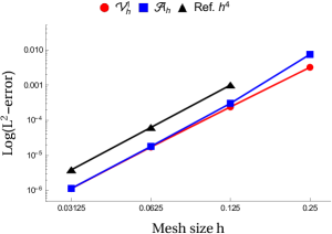
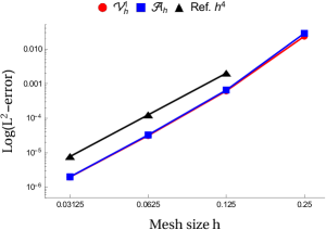
We perform -approximation over two AS- multi-patch parametrizations to numerically show that the Argyris isogeometric space maintains the polynomial reproduction properties of the entire space for the traces and normal derivatives along the interfaces, and that the space , being a subspace of , produces relative errors of the same magnitude as the entire space .
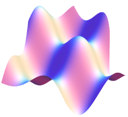
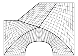
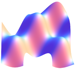
For this purpose, we consider the two AS- multi-patch parametrizations visualized in Fig. 5 (left). Both AS- geometries consist of single spline patches with , and , and are generated by using the method presented in [22]. The construction of the AS- five patch parametrization was already demonstrated in [22, Example 1]. The AS- three-patch parametrization can be obtained in an analogous manner.
For both AS- geometries we generate a sequence of nested spaces and for and by selecting the mesh size as , , and . While the bases of the Argyris spaces are simply constructed as described in Section 4, the bases of the entire spaces are obtained in the same way as in [22, Section 4.2] by means of the concept of minimal determining sets (cf. [28]). Note that in contrast to the basis functions of , the resulting basis functions of are in general not locally supported and possess a support over at least one entire interface.
We use now the basis functions for the spaces and to perform -approximation over the two AS- multi-patch parametrizations. Consider one of the spaces or , and let be the corresponding basis functions. The goal is to approximate the function
| (45) |
see Fig. 5 (middle), by the function
via minimizing the term
The isogeometric formulation of this linear problem was discussed in detail in [22, Section 4.2], and will be omitted here for the sake of brevity.
| AS- geometry | Exact solution | Relative -error |
 |
 |
 |
| Example: AS- three-patch geometry | ||
 |
 |
 |
| Example: AS- five-patch geometry | ||
Table 1 and Fig. 5 (right) report the resulting relative -errors and the estimated convergence rates for the two spaces and for the different mesh sizes . The numerical results indicate for both spaces convergence rates of optimal order in the -norm and show that resulting relative -errors are of the same magnitude for the two spaces.
| Subspace | Entire space | |||||
| AS- three-patch geometry (a) | ||||||
| e.c.r. | e.c.r. | |||||
| 1/4 | 177 | 7.46e-03 | - | 222 | 3.21e-03 | - |
| 1/8 | 729 | 3.03e-04 | 4.62 | 822 | 2.4e-04 | 3.74 |
| 1/16 | 2985 | 1.8e-05 | 4.07 | 3174 | 1.73e-05 | 3.79 |
| 1/32 | 12105 | 1.15e-06 | 3.97 | 12486 | 1.14e-06 | 3.92 |
| AS- five-patch geometry (b) | ||||||
| e.c.r. | e.c.r. | |||||
| 1/4 | 291 | 2.86e-02 | - | 372 | 2.35e-02 | - |
| 1/8 | 1211 | 6.5e-04 | 5.46 | 1376 | 6.14e-04 | 5.25 |
| 1/16 | 4971 | 3.28e-05 | 4.31 | 5304 | 3.14e-05 | 4.29 |
| 1/32 | 20171 | 2.02e-06 | 4.02 | 20840 | 1.99e-06 | 3.98 |
6 Conclusion
We presented for the class of AS- multi-patch parametrizations the construction of a basis and of an associated dual basis for the so-called Argyris isogeometric space , which generalizes the classical Argyris finite elements to multi-patch isogeometric spaces. It is a subspace of the entire isogeometric space maintaining the polynomial reproduction properties of for the traces and normal derivatives along the interfaces. This property of the subspace was shown numerically by performing -approximation over different AS- multi-patch parametrizations. The use of the Argyris space instead of the space is advantageous since the subspace has a simpler structure and allows a uniform and simple construction of the basis functions independent of the AS- domain parametrization. The construction of the basis (and of its dual basis) is based on the decomposition of the space into the direct sum of three subspaces called the patch-interior, the edge and the vertex function space. The resulting basis and the dual basis have a simple form, since the single functions are locally supported and are explicitly given by closed form representations.
This paper presents the foundation for further studies of isogeometric spaces over AS- multi-patch parametrizations, by providing a basis and corresponding projectors. A first planned topic for future research is the theoretical investigation of the properties of the space , such as approximation error and stability estimates for -refined meshes, which can be built upon a suitable dual basis. Moreover, one may also construct a basis forming a partition of unity, following the ideas presented in [12], based on local triangular Bézier surfaces at the vertices. We are also planning to extend the construction to surface domains and to use our approach to perform Kirchhoff-Love shell analysis for different linear and non-linear model configurations. Another challenging task will be the extension to volumetric domains. So far, no generalization of AS- parametrizations to volumetric domains is known.
Acknowledgments
G. Sangalli is member of the Gruppo Nazionale Calcolo Scientifico-Istituto Nazionale di Alta Matematica (GNCS-INDAM), and was partially supported by the European Research Council through the FP7 Ideas Consolidator Grant HIGEOM n.616563. This support is gratefully acknowledged.
Appendix A Proof of Lemma 5 and 6
Proof of Lemma 5.
Let . Assume (this is not true in general for boundary vertices, if so the proof below simplifies in a trivial way). On each patch , or , we can write the pull-back of and of the projection as
and
We have by definition, using the abbreviations and
and using the chain rule of differentiation, that
| (46) |
Consider the basis transformations from to and from to , with
where is the Kronecker delta. Then, recalling (23) and (25), we can rewrite the functions and in terms of the new bases:
| (47) |
and
| (48) |
Considering (47), we then have
| (49) |
using the abbreviated notation
and
we can determine all from the interpolation conditions
| (50) |
Hence, there exists a projector satisfying (39). We can reason similarly on (48), where we have
| (51) |
In fact, after inserting (50) into (51) and simplifying, we obtain (46) for . Hence, the projector also satisfies (40), which concludes the proof. ∎
Proof of Lemma 6.
We use again the abbreviated notation and , where by definition for .
Then we have
| (52) |
The active degrees-of-freedom of three terms in (52) with respect to the underlying tensor-product spline space are pictured in Figure 6.
Finally, if vanishes, then all the derivatives above are null and, by definition, , and are null. ∎
Appendix B Extension to non-uniform knots and (partially) matching meshes
Note that one can extend the presented construction easily to multi-patch domains with non-uniform meshes and partially matching interfaces. We will briefly sketch the necessary adaptions. We assume to have different spline spaces for every patch with . Every space satisfies
where is a univariate spline space of degree and regularity , having distinct inner knots
each with multiplicity and having and as boundary knots with multiplicity .
Having defined different spaces for every patch, we change Assumption 4 and Definition 9 and assume as well as . Now, in order to have a sufficiently large isogeometric space along every interface, we need that the knot meshes are (partially) matching along all interfaces.
Assumption 26.
Consider an interface , with . Assume , are in standard form for . Then the corresponding meshes are
-
1.
matching, i.e., , or
-
2.
partially matching, i.e., or .
Note that two meshes are matching along an interface, if the corresponding knots are the same. The meshes are partially matching along an interface, if the knots of one patch are a subset of the knots of the other.
The space can be constructed just as for uniform meshes. The patch-interior basis (Definition 16) needs no additional modification. The edge-interior basis (Definition 18) uses spaces and , which are built from by reducing the knot multiplicity by one or reducing the polynomial degree by one, respectively. See [21] for a construction of the complete basis for non-uniform knots. The vertex basis (Definition 21) is defined as a linear combination of patch and edge contributions and can be constructed analogously.
Appendix C Another approximating subspace
Instead of the space given in (19), one can consider a slightly larger subspace , which contains all isogeometric functions which are at the interior vertices and boundary vertices of valency and are everywhere else. The space is given by
where the indices in represents all boundary vertices of valency . In contrast to (19), different patch interior spaces, denoted by , and different edge function spaces, denoted by , are used to generate the space . A further difference is that the new edge function space will be now only taken for all interfaces, and that the vertex function space have to be only selected for all interior vertices and for all boundary vertices of valency . Below, we will present the definitions of the spaces and , which will be similar to the ones for the spaces and , see Definition 16 and 18, respectively.
Before, we will need some additional assumptions and definitions. We assume that in case of for , , the functions and are selected as . For each , , let
and
Since and are linear polynomials, and is a quadratic polynomial, we obtain that and , cf. [21]. For each , we denote by the univariate spline space of degree on the parameter domain , constructed from the open knot vector with non-empty knots spans with (mesh) size , where the inner knots , with , have multiplicity , and the inner knot has multiplicity . This means that functions of the space are on except at the inner knot , where they are only .
We first define the patch interior space . In contrast to the space , the isogeometric functions of the space need not have vanishing values and gradients at possible boundary edges of the multi-path domain , but still have vanishing values and gradients at the patch interfaces.
Definition 27.
Let , we define the space as
where the index set takes all which do not belong to the data of an interface , with , or to the data of a vertex , with .
The definition of the edge function space is based on the construction of the (entire) isogeometric space for AS- two-patch geometries presented in [21].
Definition 28.
Let , for , be an interface in standard form. Consider the univariate spline spaces and , with bases , and , respectively, where with and . For each , let be a B-spline of the space with the property which have vanishing derivatives up to second order at both interface vertices. We define the index set
and . In addition, let and . We define the space as
where
for ,
for , and
for . Let then be the subspace of , given by
Remark 10.
In contrast to the subspace , the dimension of the subspace depends on the domain parametrization. Let and let
Then, the subspace
with , would be another choice of a isogeometric subspace, and its dimension is as the dimension of the subspace independent of the domain parametrization.
References
References
- [1] J. H. Argyris, I. Fried, and D. W. Scharpf. The TUBA family of plate elements for the matrix displacement method. The Aeronautical Journal, 72(692):701–709, 1968.
- [2] F. Auricchio, L. Beirão da Veiga, A. Buffa, C. Lovadina, A. Reali, and G. Sangalli. A fully ”locking-free” isogeometric approach for plane linear elasticity problems: a stream function formulation. Comput. Methods Appl. Mech. Engrg., 197(1):160–172, 2007.
- [3] A. Bartezzaghi, L. Dedè, and A. Quarteroni. Isogeometric analysis of high order partial differential equations on surfaces. Comput. Methods Appl. Mech. Engrg., 295:446 – 469, 2015.
- [4] L. Beirão da Veiga, A. Buffa, G. Sangalli, and R. Vázquez. Mathematical analysis of variational isogeometric methods. Acta Numerica, 23:157–287, 5 2014.
- [5] D. J. Benson, Y. Bazilevs, M.-C. Hsu, and T. J.R. Hughes. A large deformation, rotation-free, isogeometric shell. Comput. Methods Appl. Mech. Engrg., 200(13):1367–1378, 2011.
- [6] M. Bercovier and T. Matskewich. Smooth Bézier Surfaces over Unstructured Quadrilateral Meshes. Lecture Notes of the Unione Matematica Italiana, Springer, 2017.
- [7] A. Blidia, B. Mourrain, and N. Villamizar. G1-smooth splines on quad meshes with 4-split macro-patch elements. Computer Aided Geometric Design, 52–53:106–125, 2017.
- [8] F. K. Bogner, R. L. Fox, and L. A. Schmit. The generation of interelement compatible stiffness and mass matrices by the use of interpolation formulae. In Proc. Conf. Matrix Methods in Struct. Mech., AirForce Inst. of Tech., Wright Patterson AF Base, Ohio, 1965.
- [9] Philippe G Ciarlet. The finite element method for elliptic problems. Classics in applied mathematics, 40:1–511, 2002.
- [10] A. Collin, G. Sangalli, and T. Takacs. Analysis-suitable G1 multi-patch parametrizations for C1 isogeometric spaces. Computer Aided Geometric Design, 47:93 – 113, 2016.
- [11] J. A. Cottrell, T.J.R. Hughes, and Y. Bazilevs. Isogeometric Analysis: Toward Integration of CAD and FEA. John Wiley & Sons, Chichester, England, 2009.
- [12] P. Dierckx. On calculating normalized Powell-Sabin B-splines. Computer Aided Geometric Design, 15(1):61–78, 1997.
- [13] G. Farin. Curves and Surfaces for Computer-Aided Geometric Design. Academic Press, 1997.
- [14] H. Gómez, V. M Calo, Y. Bazilevs, and T. J.R. Hughes. Isogeometric analysis of the Cahn–Hilliard phase-field model. Comput. Methods Appl. Mech. Engrg., 197(49):4333–4352, 2008.
- [15] H. Gomez, V. M. Calo, and T. J. R. Hughes. Isogeometric analysis of Phase–Field models: Application to the Cahn–Hilliard equation. In ECCOMAS Multidisciplinary Jubilee Symposium: New Computational Challenges in Materials, Structures, and Fluids, pages 1–16. Springer Netherlands, 2009.
- [16] D. Groisser and J. Peters. Matched Gk-constructions always yield Ck-continuous isogeometric elements. Computer Aided Geometric Design, 34:67 – 72, 2015.
- [17] J. Hoschek and D. Lasser. Fundamentals of computer aided geometric design. A K Peters Ltd., Wellesley, MA, 1993.
- [18] T. J. R. Hughes, J. A. Cottrell, and Y. Bazilevs. Isogeometric analysis: CAD, finite elements, NURBS, exact geometry and mesh refinement. Comput. Methods Appl. Mech. Engrg., 194(39-41):4135–4195, 2005.
- [19] Gašper Jaklič and Tadej Kanduč. Hermite parametric surface interpolation based on Argyris element. Computer Aided Geometric Design, 56:67–81, 2017.
- [20] M. Kapl, F. Buchegger, M. Bercovier, and B. Jüttler. Isogeometric analysis with geometrically continuous functions on planar multi-patch geometries. Comput. Methods Appl. Mech. Engrg., 316:209 – 234, 2017.
- [21] M. Kapl, G. Sangalli, and T. Takacs. Dimension and basis construction for analysis-suitable G1 two-patch parameterizations. Computer Aided Geometric Design, 52–53:75 – 89, 2017.
- [22] M. Kapl, G. Sangalli, and T. Takacs. Construction of analysis-suitable G1 planar multi-patch parameterizations. Computer-Aided Design, 97:41 – 55, 2018.
- [23] M. Kapl, V. Vitrih, B. Jüttler, and K. Birner. Isogeometric analysis with geometrically continuous functions on two-patch geometries. Comput. Math. Appl., 70(7):1518 – 1538, 2015.
- [24] K. Karčiauskas, T. Nguyen, and J. Peters. Generalizing bicubic splines for modeling and IGA with irregular layout. Computer-Aided Design, 70:23–35, 2016.
- [25] J. Kiendl, Y. Bazilevs, M.-C. Hsu, R. Wüchner, and K.-U. Bletzinger. The bending strip method for isogeometric analysis of Kirchhoff-Love shell structures comprised of multiple patches. Comput. Methods Appl. Mech. Engrg., 199(35):2403–2416, 2010.
- [26] J. Kiendl, K.-U. Bletzinger, J. Linhard, and R. Wüchner. Isogeometric shell analysis with Kirchhoff-Love elements. Comput. Methods Appl. Mech. Engrg., 198(49):3902–3914, 2009.
- [27] J. Kiendl, M.-Ch. Hsu, M. C. H. Wu, and A. Reali. Isogeometric Kirchhoff–Love shell formulations for general hyperelastic materials. Comput. Methods Appl. Mech. Engrg., 291:280 – 303, 2015.
- [28] M.-J. Lai and L. L. Schumaker. Spline functions on triangulations, volume 110 of Encyclopedia of Mathematics and its Applications. Cambridge University Press, Cambridge, 2007.
- [29] M-J-Jun Lai and L. L. Schumaker. Spline functions on triangulations. Cambridge University Press, 2007.
- [30] J. Liu, L. Dedè, J. A. Evans, M. J. Borden, and T. J. R. Hughes. Isogeometric analysis of the advective Cahn–Hilliard equation: Spinodal decomposition under shear flow. Journal of Computational Physics, 242:321 – 350, 2013.
- [31] B. Mourrain, R. Vidunas, and N. Villamizar. Dimension and bases for geometrically continuous splines on surfaces of arbitrary topology. Computer Aided Geometric Design, 45:108 – 133, 2016.
- [32] T. Nguyen, K. Karčiauskas, and J. Peters. A comparative study of several classical, discrete differential and isogeometric methods for solving poisson’s equation on the disk. Axioms, 3(2):280–299, 2014.
- [33] T. Nguyen, K. Karčiauskas, and J. Peters. finite elements on non-tensor-product 2d and 3d manifolds. Applied Mathematics and Computation, 272:148 – 158, 2016.
- [34] M.A. Scott, R.N. Simpson, J.A. Evans, S. Lipton, S.P.A. Bordas, T.J.R. Hughes, and T.W. Sederberg. Isogeometric boundary element analysis using unstructured t-splines. Comp. Methods Appl. Mech. Engrg., 254:197 – 221, 2013.
- [35] A. Tagliabue, L. Dedè, and A. Quarteroni. Isogeometric analysis and error estimates for high order partial differential equations in fluid dynamics. Computers & Fluids, 102:277 – 303, 2014.
- [36] T. Takacs. Construction of smooth isogeometric function spaces on singularly parameterized domains. In International Conference on Curves and Surfaces, pages 433–451. Springer, 2014.
- [37] T. Takacs and B. Jüttler. H2 regularity properties of singular parameterizations in isogeometric analysis. Graphical Models, 74(6):361–372, 2012.
- [38] D. Toshniwal, H. Speleers, R. Hiemstra, and T. J. R. Hughes. Multi-degree smooth polar splines: A framework for geometric modeling and isogeometric analysis. Comput. Methods Appl. Mech. Engrg., 316:1005–1061, 2017.
- [39] D. Toshniwal, H. Speleers, and T. J. R. Hughes. Analysis-suitable spline spaces of arbitrary degree on unstructured quadrilateral meshes. Technical Report 16, Institute for Computational Engineering and Sciences (ICES), 2017.
- [40] D. Toshniwal, H. Speleers, and T. J. R. Hughes. Smooth cubic spline spaces on unstructured quadrilateral meshes with particular emphasis on extraordinary points: Geometric design and isogeometric analysis considerations. Comput. Methods Appl. Mech. Engrg., 327:411–458, 2017.
- [41] M. Wu, B. Mourrain, A. Galligo, and B. Nkonga. Hermite type spline spaces over rectangular meshes with complex topological structures. Communications in Computational Physics, 21(3):835–866, 2017.