Fast and reliable inference algorithm for hierarchical stochastic block models

I Introduction

Network clustering reveals the organization of a network or corresponding complex system with elements represented as vertices and interactions as edges in a (directed, weighted) graph. Although the notion of clustering can be somewhat loose, network clusters or groups are generally considered as nodes with enriched interactions Newman:2001wm ; Leskovec:2008im and edges sharing common patterns Ahn:2010dj . Statistical inference often treats groups as latent variables, with observed networks generated from latent group structure, termed a stochastic block model Nowicki:2001id . Regardless of the definitions, statistical inference can be either translated to modularity maximization, which is provably an NP-complete problem Brandes:2008bu .

Here we present scalable and reliable algorithms that recover hierarchical stochastic block models fast and accurately. Our algorithm scales almost linearly in number of edges, and inferred models were more accurate that other scalable methods.

II Models

Stochastic block model

We represent a network data as an adjacency matrix $A$, where each element $A_{ij}$ captures the relationship between vertices $i,j\in V$. Let $n$ be a number of vertices, $n=|V|$, and $m$ be a number of (un)directed edges, or non-zero entries of (upper triangular) $A$. For a binary and undirected network, $A_{ij}$ takes on a value $1$ if $i$ and $j$ interact, $0$ otherwise. We assume that the set $V$ decomposes into an arbitrary $K$ disjoint subsets. We give a unique index $1,\ldots,K$ to these subsets. For simplicity let $g_{i}$ denotes membership mapping of vertex $i$ to a certain group, with $g_{i}\in[K]$. Assume each group (or block) is identifiable by a $K\times K$ block matrix $\boldsymbol{\theta}$ and $\theta_{ab}\in[0,1]$ for all ${a,b\in[K]\times[K]}$. We can define the data likelihood as

$$p(A|g,\theta)=\prod_{i<j}\theta_{g_{i}g_{j}}^{A_{ij}}(1-\theta_{g_{i},g_{j}})^{1-A_{ij}}.$$

Degree-corrected stochastic block model

In some situations, a degree-corrected stochastic block model (DSBM) provides more appealing group structures in a real-world network Karrer:2010vd . Again, we represent a network as an adjacency matrix $A$; a vertex set $V$ decomposes into $K$ disjoint subsets; the membership function is $g$, ${g:\,V\to[K]}$. However, $A_{ij}$ may takes on values of non-negative real number, and block-block relationships are captured by a $K\times K$ matrix $\boldsymbol{\lambda}$ and $\lambda_{ab}\in\mathbb{R}^{+}$ for all ${a,b\in[K]\times[K]}$.

Our DSBM generalizes a regular SBM, weighting edges based on degrees of endpoints by $\rho_{ij}$ for each $A_{ij}$. Here we define $\rho_{ij}\equiv d_{i}d_{j}/\sum_{j^{\prime}}d_{j^{\prime}}$. Note the denominator determines the scaling of edge weight, but does not strongly influence inference results. We define the data likelihood to have each block-block relationship follow the Poisson distribution:

$$p(A|g,\lambda)=\prod_{i<j}\frac{(\lambda_{g_{i},g_{j}}\rho_{ij})^{A_{ij}}}{A_{ij}!}e^{-\lambda_{g_{i},g_{j}}\rho_{ij}}.$$

Hierarchical group-group structure

Extensive empirical studies such as Leskovec:2008im suggest that the size of a group is limited to a certain number, meaning that ${n/K<\infty}$ and ${K\to\infty}$ as ${n\to\infty}$. Therefore a full modeling of the block matrices $\boldsymbol{\lambda}$ and $\boldsymbol{\theta}$ is inherently formidable Choi:2012ip since $K^{2}$ can easily exceed $n$ and $m$. However, most state-of-the-art algorithms require $O(K^{2})$ operations per pair and iteration (e.g., Airoldi:2008wi ), which essentially scales in $O(n^{2}K^{2})\approx O(n^{4})$. A model can be reduced that may include only within-group relationships, e.g., diagonalization of the matrix $\boldsymbol{\theta}$ Gopalan:2012vi , so that we achieve $O(mK)$ runtime where $m$ is number of edges. This strategy is useful if groups are identifiable by just “within-group” edges, and edges between groups are sampled with some background probability.

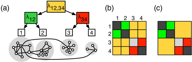
Figure 1: Hierarhical stochastic block model. (a) We assume that group-group relationships are shared hierarchically. (b) A full block matrix. (c) A shrunken block matrix by the hierarchical model.

Hierarchical assumption provides balance between the full and the diagonal block-block relationships. We adopt the idea of Clauset:2008fx and model the hierarchical group-group relations by a binary dendrogram (see Fig.1). For instance, the relationship between group $a$ and $b$ is captured by lowest common ancestor $\rm LCA(a,b)$ in the binary dendrogram and associated parameters. The model complexity of hierarchical structure scales in $O(K)$ while modeling group-group interactions.

For the hierarchical SBM (hSB), the likelihood function is defined

$$p(A|g,\boldsymbol{\theta})=\prod_{i<j}\theta_{\rm LCA(g_{i},g_{j})}^{A_{ij}}(1-\theta_{\rm LCA(g_{i},g_{j})})^{1-A_{ij}}$$ (1)

where the $\theta$ parameters follow the conjugate Beta distribution,

$$p(\theta|a_{0},b_{0})=\mathsf{Beta}(\theta|a_{0},b_{0})=\frac{\Gamma(a_{0}+b_{0})}{\Gamma(a_{0})\Gamma(b_{0})}\theta^{a_{0}-1}(1-\theta)^{b_{0}-1}.$$

For the hierarchical DSBM (hDSB), the likelihood function is defined

$$p(A|g,\lambda)=\prod_{i<j}\frac{(\lambda_{\rm LCA(g_{i},g_{j})}\rho_{ij})^{A_{ij}}}{A_{ij}!}e^{-\lambda_{\rm LCA(g_{i},g_{j})}\rho_{ij}},$$ (2)

where the rate parameters follow the Gamma distribution,

$$p(\lambda|a_{0},b_{0})=\mathsf{Gam}(\lambda|a_{0},b_{0})=\frac{b_{0}^{a_{0}}}{\Gamma(a_{0})}\lambda^{a_{0}-1}e^{-\lambda b_{0}}.$$

III Model inference

III.1 Variational Bayes inference

It is intractable to search over all binary dendrogram models. Instead, we restrict the model space to a class of complete binary trees with a fixed yet sufficiently deep depth. We then apply variational inference algorithms: mean-field approximation Xing:2003ua and locally collapsed variational inference Wang:2012uu .

We rewrite the likelihood of a tree model $\mathcal{T}$ (Eq.2) by introducing latent variables, $z_{ia}$ indicating membership of a vertex $i$ in a group $a$ if $z_{ia}=1$, otherwise $z_{ia}=0$.

$$p(A|z,\lambda)=\prod_{i<j}\prod_{r\in\mathcal{T}}\left[\frac{\lambda_{r}\rho_{ij}}{A_{ij}!}e^{-\lambda_{r}\rho_{ij}}\right]^{z_{ia}z_{jb}\mathbb{1}_{\{\rm LCA(a,b)=r\}}}$$

We approximate the posterior distribution of $z$ and $\lambda$ by the following surrogate distribution:

$$q(z,\lambda|\mu,\alpha,\beta) = \prod_{i=1}^{n}q(\mathbf{z}_{i}|\mu_{i})\prod_{r\in\mathcal{T}}q(\lambda_{r}|\alpha_{r},\beta_{r})$$ (3)

where $q(\mathbf{z}_{i}|\mu_{i})=\prod_{k=1}^{K}\mu_{ia}^{z_{ia}}$ and $q(\lambda_{r}|\alpha_{r},\beta_{r})=\mathsf{Gam}(\lambda_{r}|\alpha_{r},\beta_{r})$. As in Wang:2012uu , we distinguish random variables $\{\mathbf{z}_{i}\}$ as local variables and $\{\lambda_{r}\}$ as global variables.

Global update

Given $\left\langle z_{ia}\right\rangle\equiv\mu_{ia}$, by the generalized mean-field theory Xing:2003ua , we have variational distributions $q(\lambda_{r}|\alpha_{r},\beta_{r})$, for all $r$, characterized by

$$\alpha_{r}=a_{0}+\sum_{a,b}\sum_{i<j}\mathbb{1}_{\{r=\rm LCA(a,b)\}}\mu_{ia}\mu_{jb}A_{ij},\quad\beta_{r}=b_{0}+\sum_{a,b}\sum_{i<j}\mathbb{1}_{\{r=\rm LCA(a,b)\}}\mu_{ia}\mu_{jb}\rho_{ij}.$$ (4)

We can take expectation with respect to the variational Gamma distributions, ${\left\langle\lambda_{r}\right\rangle=\alpha_{r}/\beta_{r}}$ and ${\left\langle\ln\lambda_{r}\right\rangle=\psi(\alpha_{r})-\ln\beta_{r}}$, where $\psi(\cdot)$ denotes the digamma function. We let

$$\eta_{r}\equiv(\ln\lambda_{r},-\lambda_{r})^{\top}$$ (5)

for convenience.

Local update by mean-field theory

Let us consider that we update the probability $\mu_{i}$ of assignment of a vertex $i$ to a certain group $a$, given all other latent assignments ${\{\mu_{j}:\,j\neq i\}}$ and the global variables fixed. Note that this probability depends on the global variables $\eta_{r}$ located along the path from the leaf $a$ to the root of the tree model, which we denote by $\Pi(a)$.

For simplicity, let

$$d_{ia}\equiv\sum_{j}A_{ij}\mu_{ja},\quad\mathbf{s}_{ia}\equiv(d_{ia},\,\sum_{j}\mu_{ja}\rho_{ij})^{\top}.$$ (6)

At some $r\in\Pi(a)$, we may use the aggregated statistics:

$$\mathbf{s}_{ir}\equiv\sum_{b}\mathbb{1}_{\{r=\rm LCA(a,b)\}}\mathbf{s}_{ib},$$ (7)

which allows us to write the update equation sufficiently as

$$\mu_{ia}\propto\exp\{\sum_{r\in\Pi(a)}\left\langle\eta_{r}\right\rangle^{\top}\mathbf{s}_{ir}\}$$ (8)

subject to $\sum_{a=1}^{K}\mu_{ia}=1$ and $\mu_{ia}\geq 0$.

Local update by collapsed variational inference

Alternatively, we may update $\mu_{ia}$ by collapsing the global variables with respect to the global variational distributions. Again, we consider assigning a vertex $i$ to group $a$ and use $\mathbf{s}_{ir}$ (Eq.7) collected along the path $\Pi$ from the root of the tree to the group $a$. However, instead of using the expected natural parameters (Eq.5), we integrate them out.

$$\mu_{ia}\propto\prod_{r\in\Pi(a)}\left\langle p(\mathbf{s}_{ir}|\lambda_{r})\right\rangle_{q(\lambda|\alpha_{r},\beta_{r})}$$ (9)

where

$$\left\langle p(\mathbf{s}_{ir}|\lambda_{r})\right\rangle_{q(\lambda|\alpha_{r},\beta_{r})}\propto\int\exp\{\eta_{r}^{\top}\mathbf{s}_{ir}\}q(\eta_{r}|\alpha_{r},\beta_{r})\,d\lambda_{r}.$$

Since our model space has fixed size, we need not sample as proposed in Wang:2012uu , but just normalize $\mu_{i}$ to satisfy the constraints: $\sum_{k}\mu_{ia}=1$ and $\mu_{ia}\geq 0$.

III.2 Dynamic programming

The overall algorithm alternates between global and local updates. We approximate $q(\lambda_{r}|\alpha_{r},\beta_{r})$ by Eq. 4, then locally update $q(\mathbf{z}_{i}|\mu_{i})$ by Eq. 8 for meanfield, or 9 for locally collapsed variational inference.

Lazy evaluation of the sufficient statistics

To have it efficiently evaluate required statistics in the global update (Eq.4), we calculate the following statistics at the leaf-level,

$$d_{ia}=\sum_{j}A_{ij}\mu_{ja},\quad n_{ia}=\mu_{ia},\quad{\rm vol}_{a}=\sum_{i}\mu_{ia}d_{i},$$

then, for internal $r$, we can easily accumulate them using lower-level results,

$$d_{ir}=d_{i{\rm left}(r)}+d_{i{\rm right}(r)},\quad n_{ir}=n_{i{\rm left}(r)}+n_{i{\rm right}(r)},\quad{\rm vol}_{r}={\rm vol}_{{\rm left}(r)}+{\rm vol}_{{\rm right}(r)}.$$

We can rewrite the update equations (Eq.4) with respect to $d,n,{\rm vol}$ as follows. At the leaf group $a$,

$$\alpha_{a}=a_{0}+\sum_{i}d_{ia}\mu_{ia},\quad\beta_{a}=b_{0}+\frac{1}{4m}\sum_{i}d_{i}\mu_{ia}({\rm vol}_{a}-d_{i}\mu_{ia})$$

and for internal group $r$,

$$\alpha_{r}=a_{0}+\sum_{i}n_{i{\rm left}(r)}d_{i{\rm right}(r)},\quad\beta_{r}=b_{0}+\frac{1}{2m}\sum_{i}d_{i}n_{i{\rm left}(r)}({\rm vol}_{{\rm right}(r)}-d_{i}n_{i{\rm right}(r)}).$$

Deterministic local update

In practice, a majority of vertices can play a single role, i.e., $\left\langle\mathbf{z}_{i}\right\rangle$ has only one non-zero element filled with the value $1$. We evaluate $\mu_{i}$ by (Eq.8) or (Eq.9). Then we set $\mu_{ia^{*}}=1$ for $a^{*}=\arg\max_{a}\sum_{r\in\Pi(a)}\left\langle\eta_{r}\right\rangle\mathbf{s}_{ir}$; $mu_{ia}=0$ for $a\neq a^{*}$.

Hierarchical group structure allows us to efficiently search for the maximum assignments of vertices. While we perform a depth-first search over the binary tree model, the algorithm keeps track of maximum score $M$, corresponding group assignment $k$, and sufficient statistics $\mathbf{s}$ (See Alg.1 for details).

repeat

     for all $i\in V$ do

         $d_{ik}\leftarrow\sum_{j}A_{ij}\mu_{jk}$ for all $k$

         $(M,k_{\rm max},\mathbf{s})\leftarrow$ maxGradPath(root of ${\cal T}$)

         $\forall k\neq k_{\rm max},\,\mu_{ik}\leftarrow 0$ but $\mu_{ik_{\rm max}}\leftarrow 1$

     end for

until convergence of $\{n_{k}\}$

function maxGradPath($r$)

     if $r$ is leaf-level, cluster $k$ then

         $\mathbf{s}\leftarrow(d_{ik},d_{i}{\rm vol}[k]/2m)$

         $M\leftarrow\left\langle\eta_{k}\right\rangle^{\top}\mathbf{s}$ (Eq.8), or $\ln\left\langle p(\mathbf{s}|\lambda)\right\rangle_{q(\lambda|\alpha_{k},\beta_{k})}$ (Eq.9)

         return $(M,k,\mathbf{s})$

     else

         $(M_{\rm left},k_{\rm left},\mathbf{s}_{\rm left})\leftarrow$ maxGradPath(left($r$))

         $(M_{\rm right},k_{\rm right},\mathbf{s}_{\rm right})\leftarrow$ maxGradPath(right($r$))

         $M_{\rm left}\leftarrow M_{\rm left}+\left\langle\eta_{r}\right\rangle^{\top}\mathbf{s}_{\rm right}$ (Eq.8), or $\ln\left\langle p(\mathbf{s}_{\rm right}|\lambda)\right\rangle_{q(\lambda|\alpha_{r},\beta_{r})}$ (Eq.9)

         $M_{\rm right}\leftarrow M_{\rm right}+\left\langle\eta_{r}\right\rangle^{\top}\mathbf{s}_{\rm left}$ (Eq.8), or $\ln\left\langle p(\mathbf{s}_{\rm left}|\lambda)\right\rangle_{q(\lambda|\alpha_{r},\beta_{r})}$ (Eq.9)

         $M_{\rm max}\leftarrow\max\,\{M_{\rm left},M_{\rm right}\}$, and $k_{\rm max}\leftarrow\arg\max_{k^{\prime}\in\{{\rm left,right}\}}\,M_{k^{\prime}}$

         return $(M_{\rm max},k_{\rm max},\mathbf{s}_{\rm left}+\mathbf{s}_{\rm right})$

     end if

end function

Alg 1 Deterministic latent variable inference

Probabilistic local update

The similar lazy-evaluation approach can be applied to the probabilistic latent variable update for $\mu_{ia}$. With memoization of partial log-scores (Eq.9 or Eq.8), we can exactly evaluate $\mu$ within two passes of tree traversal (see Alg.2 for details).

repeat

     for all $i\in[n]$ do

         $d_{ik}\leftarrow\sum_{j}A_{ij}\mu_{jk}$ for all $k$

         calcGradPath(root of ${\cal T}$)

         sumGradPath(root of ${\cal T}$, 0)

         $\mu_{ik}\propto\exp\{\nabla[k]\}$

     end for

until convergence

function calcGradPath($r$)

     if $r$ is leaf-level, cluster $k$ then

         $\mathbf{s}\leftarrow(d_{ik},d_{i}{\rm vol}[k]/2m)$

         return $\mathbf{s}$

     else

         $\mathbf{s}_{\rm left}\leftarrow$ calcGradPath(left($r$))

         $\mathbf{s}_{\rm right}\leftarrow$ calcGradPath(right($r$))

         $\delta_{\rm left}[r]\leftarrow\left\langle\eta_{r}\right\rangle^{\top}\mathbf{s}_{\rm right}$ (Eq.8), or $\ln\left\langle p(\mathbf{s}_{\rm right}|\lambda)\right\rangle_{q(\lambda|\alpha_{r},\beta_{r})}$ (Eq.9)

         $\delta_{\rm right}[r]\leftarrow\left\langle\eta_{r}\right\rangle^{\top}\mathbf{s}_{\rm left}$ (Eq.8), or $\ln\left\langle p(\mathbf{s}_{\rm left}|\lambda)\right\rangle_{q(\lambda|\alpha_{r},\beta_{r})}$ (Eq.9)

         return $(\mathbf{s}_{\rm left}+\mathbf{s}_{\rm right})$

     end if

end function

function sumGradPath($r,\alpha$)

     if $r$ is bottom-level, cluster $k$ then

         $\mathbf{s}\leftarrow(d_{ik},n_{k})$

         $\nabla[k]\leftarrow\alpha+\left\langle\eta_{k}\right\rangle^{\top}\mathbf{s}$ (Eq.8), or $\ln\left\langle p(\mathbf{s}|\lambda)\right\rangle_{q(\lambda|\alpha_{k},\beta_{k})}$ (Eq.9)

     else

         sumGradPath(left($r$), $\alpha+\delta_{\rm left}$[r])

         sumGradPath(right($r$), $\alpha+\delta_{\rm right}$[r])

     end if

end function

Alg 2 Recursive latent variable inference

Both global and local update steps scale in $O(mK)$. The deterministic update converges faster (in $5$ to $10$ iterations), while the probabilistic one converges in tens of iterations.

Pruning unnecessarily branching subtrees

Allowing sufficient depth of the tree model, we may generate an over-complicated model fitted to noisy observation. To reduce model complexity, we apply final pruning steps. At each subtree of the full model, we compared this subtree with the collapsed model under the single group. We determine whether to collapse or not via the Bayse factor, or log-ratio of the marginal likelihood Heller:2005el . This automatically determines the number of groups from the data.

Initialization

Variational inference algorithms not necessarily guarantee the convergence to global optima. To avoid bad local optima, we may restart the algorithm multiple times from random configuration. However, the model space grows super-exponentially and an algorithm may require exponentially many random restarts. Instead, we found that iterative bisections of network provide a good starting point. Since each bisection using the deterministic inference with $2$ groups can be completed in $O(m)$, we can finish the whole initialization in $O(m\log K)$.

Approximation for speed up

Although $O(mK)$ runtime is practical for small $K$, a network of 10,000 nodes and 100,000 edges could have $K$ as large as 1000. Therefore, full computation of each variational update could make the overall algorithm scales essentially in $O(mn)$ (if $O(n)=O(K)$). We may reduce $m$ as in the previous work Gopalan:2012vi by stochastic variational inference. Here, we address different aspect, reducing $K$ to some $k^{*}\ll K$.

Suppose we want to re-assign a vertex $i$ by evaluating ${\{\mu_{ik}:\,k\in[K]\}}$. In assortative networks, vertices tend to form a group only with connected vertices. This allows us to locally carry out the computation of latent and global updates. Let $U$ be a subset of leaf groups, to which the vertex $i$ is connected, i.e., $U=\{k\in[K]:d_{ik}>0\}$ (see Eq.6). Let $k_{\min}=\min U$ and $k_{\max}=\max U$. With a proper initial configuration (e.g., iterative bisections), we get $|U|\ll K$. Then, we can restrict maxGradPath (Alg.1), and calcGradPath and sumGradPath (Alg.2) to a small subtree. We can call them from $\rm LCA(k_{\min},k_{\max})$. Moreover, this locality can be determined in constant time.

IV Results and Discussions

Simulation study

The hDSB outperforms in various benchmark networks. We generated sparse network data with average degree $10$ and maximum degree $100$ using the LFR benchmark Lancichinetti:2008ge . We also tested on benchmark networks with higher degrees (e.g., $30,50,100$) and found that hDSB was still the best performing algorithm, and its performance can easily attain to the mutual information $1$. However, this setting is far from real-world networks, so we omit the result. With the fixed degree distribution, we varied size of the networks ($5000,10000$). We also varied the maximum size of groups ($20,50,100,150$) while fixing the minimum size to $10$. Although our method can provide mixed membership probability, we did not allow mixed membership to compare with other community detection methods.

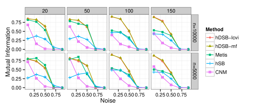
Figure 2: The benchmark result. x-axis: noise parameter (the $\mu$ parameter of LFR Lancichinetti:2008ge ); y-axis: normalized mutual information Lancichinetti:2009dy ; Top titles: the maximum size of a group; Right titles: total number of vertices. See the text for details.

Fig.2 compares hDSB with locally collapsed variational inference (hDSB-lcvi), hDSB with mean-field (hDSB-mf), $k$-metis provided with true $K$ Karypis:1998by (Metis), hSB with mean-field (hSB), and modularity maximization Clauset:2004uy (CNM). We measured the normalized mutual information (NMI) Lancichinetti:2009dy between the inferred and the ground truth groups. The NMI scales in between $0$ and $1$, and higher value means higher similarity.

In overall, the performance of hDSB dominates the other methods. The effect of different latent variable inference was not so significant. For networks with balanced group structure, with the maximum group size $\leq 50$, Metis algorithm performs nearly as well as hDSB. However, it requires the number of groups as a parameter, and real-world networks may contain heterogeneous group structures. The degree-correction provides more realistic group structure than regular SBM; in fact, we found that it prevents from over-segmentation. Not surprisingly, since CNM algorithm relies on local greedy steps, it was most sensitive to noise and resolution limit problem Fortunato:2007js (under-segmentation).

Cross-validation: link prediction tests

We used 6 real-world datasets (2 biological and 4 social networks): NCAA: NCAA college football network Girvan:2002ez ; NetSci: coauthorship network on the network science Newman:2006uo ; Hep-Th: co-authorship network on the High-Energy Theory Archive Newman:2001wm ; Cond: co-authorship network on the Condensed Matter Archive Newman:2001wm ; Reactome: co-reaction network Croft:2011ga ; CoExp: Genemania co-expression network Mostafavi:2008bz .

With true group structure unknown, performance may be assessed by link prediction. We removed links chosen uniformly from the observed network. For large networks, such as Hep-TH, Cond, CoExp, we chose the same number of non-links. For smaller networks, NCAA, NetSci, Reactome, we chose non-links while preserving the original ratio of links to non-links. We preprocessed the networks by iteratively removing vertices with degree $\leq 2$, since these vertices do not form a group.

In addition to the methods used in the benchmark study, we considered the sampling method of hierarchical random graph Clauset:2008fx (HRG) and the link community optimization by the maximum likelihood Ball:2011wz (LC). These methods do not provide a fixed group structure, rather scores $s_{ij}$ for a pair $ij$, and a high scoring pair means a possible link. For the algorithms that provide a group structure, we estimated the score $s_{ij}$ by group-wise frequency,

$$\hat{\theta}_{ab}=\frac{\textrm{\# links observed between one end in group $a$ and the other in group $b$}}{\textrm{\# possible links between groups $a$ and $b$}}.$$

For instance, a pair $ij$ takes $\hat{\theta}_{ab}$ as a score if $i$ and $j$ belong to groups $a$ and $b$ respectively. We allowed 10 random restarts for LC method. Metis and LC require pre-specified number of blocks or colors. We performed discrete grid search over the parametric space and reported the best results. As a summary statistic, we estimated the area under the precision-recall curve (AUPRC) Davis:2006kr . AUPRC scales in $[0,1]$ on the small datasets (NCAA, NetSci, and Reactome); $[0.5,1]$ on the large networks (Hep-Th, Cond2005, CoExp).

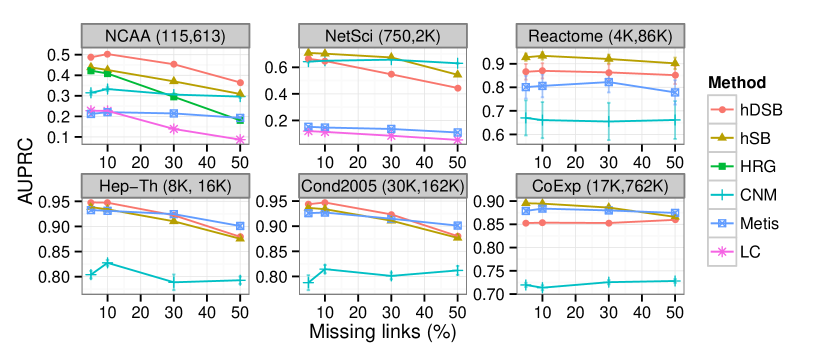
Figure 3: The missing link prediction results. x-axis: a fraction of missing links; y-axis: area under the precision recall curve; (n,m): $n=$ number of vertices and $m=$ number of edges.

Fig.3 shows the results on these networks. Either hDSB or hSB was consistently top-ranked on all datasets over all range of missing links. Notably hSB performed best in some networks. We may conclude that groups of hSB are as robust as hDSB, and groups of the benchmark networks can be reasonably further decomposed into smaller groups. In the NCAA network, our algorithms even outperformed the exhaustive sampling method (HRG). Link community optimization (LC) works poorly in both scalability and accuracy if a network consists of many groups. It appears that the proposed algorithm of Ball & Newman Ball:2011wz can easily overfit the training data. A similar argument was also made previously Gopalan:2012vi .

Runtime

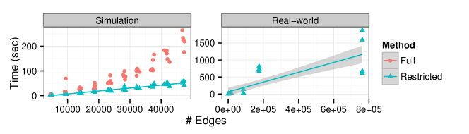
Figure 4: Runtime of the algorithms.

Fig.4 shows runtime as a function of number of edges. We ran Alg. 2 with full or restricted calculation. While the full version increases almost quadratically (red dots), runtime of the restricted grows linearly (blue triangles) on simulation and real-world networks. In terms of accuracy, the restricted version worked equally well.

Acknowledgments

Source codes available at https://code.google.com/p/hsblock/ or from the authors by e-mail.

References

• [1] Yong-Yeol Ahn, Jamesย P Bagrow, and Sune Lehmann. Link communities reveal multiscale complexity in networks. Nature, 466(7307):761โ€“764, August 2010.
• [2] Edoardoย M Airoldi, Davidย M Blei, Stephenย E. Fienberg, and Ericย P. Xing. Mixed membership stochastic blockmodels. Journal of Machine Learning Research, 9:1981โ€“2014, October 2008.
• [3] Brian Ball, Brian Karrer, and M.ย E.ย J. Newman. Efficient and principled method for detecting communities in networks. Physical Review E, 84(3-2):036103, September 2011.
• [4] Uย Brandes, Dย Delling, Mย Gaertler, Rย Gorke, Mย Hoefer, Zย Nikoloski, and Dย Wagner. On Modularity Clustering. IEEE Transactions on Knowledge and Data Engineering, 20(2):172โ€“188, 2008.
• [5] Dย S Choi, Pย J Wolfe, and Eย M Airoldi. Stochastic blockmodels with a growing number of classes. Biometrika, 99(2):273โ€“284, January 2012.
• [6] Aaron Clauset, Cristopher Moore, and M.ย E.ย J. Newman. Hierarchical structure and the prediction of missing links in networks. Nature, 453(7191):98โ€“101, 2008.
• [7] Aaron Clauset, M.ย E.ย J. Newman, and Cristopher Moore. Finding community structure in very large networks. Physical review E, Statistical, nonlinear, and soft matter physics, 70(6 Pt 2):66111, 2004.
• [8] David Croft, Gavin Oโ€™Kelly, Guanming Wu, Robin Haw, Marc Gillespie, Lisa Matthews, Michael Caudy, Phani Garapati, Gopal Gopinath, Bijay Jassal, Steven Jupe, Irina Kalatskaya, Shahana Mahajan, Bruce May, Nelson Ndegwa, Esther Schmidt, Veronica Shamovsky, Christina Yung, Ewan Birney, Henning Hermjakob, Peter Dโ€™Eustachio, and Lincoln Stein. Reactome: a database of reactions, pathways and biological processes. Nucleic Acids Res, 39(Database issue):D691โ€“7, January 2011.
• [9] Jesse Davis and Mark Goadrich. The relationship between Precision-Recall and ROC curves. In ICML โ€™06: Proceedings of the 23rd international conference on Machine learning. ACM, June 2006.
• [10] Santo Fortunato and Marc Barthelemy. Resolution limit in community detection. Proc Natl Acad Sci USA, 104(1):36โ€“41, 2007.
• [11] M.ย Girvan and M.ย E.ย J. Newman. Community structure in social and biological networks. Proceedings of the National Academy of Sciences, 99(12):7821โ€“7826, January 2002.
• [12] Prem Gopalan, David Mimno, Seanย M Gerrish, Michaelย J Freedman, and Davidย M Blei. Scalable Inference of Overlapping Communities. Advances in Neural Information Procesing Systems (NIPS), 2012.
• [13] Katherineย A Heller and Zoubin Ghahramani. Bayesian Hierarchical Clustering. In Proceedings of the 22nd international conference on Machine learning - ICML โ€™05, pages 297โ€“304, New York, New York, USA, 2005. ACM Press.
• [14] Brian Karrer and M.ย E.ย J. Newman. Stochastic blockmodels and community structure in networks. Physical Review E, pageย 11, 2010.
• [15] George Karypis and Vipin Kumar. A Fast and High Quality Multilevel Scheme for Partitioning Irregular Graphs. SIAM J. Sci. Comput., 20(1):359โ€“392, 1998.
• [16] Andrea Lancichinetti, Santo Fortunato, and Jรกnos Kertย e sz. Detecting the overlapping and hierarchical community structure in complex networks. New Journal of Physics, 11(3):033015, 2009.
• [17] Andrea Lancichinetti, Santo Fortunato, and Filippo Radicchi. Benchmark graphs for testing community detection algorithms. Phys. Rev. E, 78(4):46110, 2008.
• [18] Jure Leskovec, Kevinย J. Lang, Anirban Dasgupta, and Michaelย W. Mahoney. Statistical properties of community structure in large social and information networks. In WWW โ€™08: Proceeding of the 17th international conference on World Wide Web. ACM, April 2008.
• [19] Sara Mostafavi, Debajyoti Ray, David Warde-Farley, Chris Grouios, and Quaid Morris. GeneMANIA: a real-time multiple association network integration algorithm for predicting gene function. Genome biology, 9 Suppl 1:S4, 2008.
• [20] M.ย E.ย J. Newman. The structure of scientific collaboration networks. Proceedings of the National Academy of Sciences, 98(2):404โ€“409, January 2001.
• [21] M.ย E.ย J. Newman. Modularity and community structure in networks. Proc Natl Acad Sci USA, 103(23):8577โ€“8582, 2006.
• [22] Krzysztof Nowicki and Tom Aย B Snijders. Estimation and prediction for stochastic blockstructures. Journal of the American Statistical Association, 96(455):1077โ€“1087, 2001.
• [23] Chong Wang and Davidย M Blei. Truncation-free Stochastic Variational Inference for Bayesian Nonparametric Models. In Advances in Neural Information Procesing Systems (NIPS). Computer Science Department, Princeton University, 2012.
• [24] Ericย P. Xing, Michaelย I Jordan, and Stuart Russell. A generalized mean field algorithm for variational inference in exponential families. In Uncertainty in Artificial Intelligence (UAI 2003). Computer Science Division, Unifersity of California Berkeley, 2003.