On the Quasi-Stationary Distribution of the Shiryaev MartingaleA. S. Polunchenko, S. Martínez, and J. San Martín \WarningFilterrefcheckUnused label ‘sec:intro’
A Note on the Quasi-Stationary Distribution
of the Shiryaev Martingale on the Positive Half-Line††thanks: Submitted to the editors DATE.
\fundingThe effort of A. S. Polunchenko was partially supported by the Simons Foundation via a Collaboration Grant in Mathematics under Award # 304574.
Abstract
We obtain a closed-form formula for the quasi-stationary distribution of the classical Shiryaev martingale diffusion considered on the positive half-line with fixed; the state space’s left endpoint is assumed to be the killing boundary. The formula is obtained analytically as the solution of the appropriate singular Sturm–Liouville problem; the latter was first considered in [7, Section 7.8.2], but has heretofore remained unsolved.
keywords:
Quasi-stationary distribution, Shiryaev martingale, Whittaker functions60J60, 60F99, 33C15
1 Introduction and problem formulation
This work centers around the stochastic process known as the Shiryaev martingale. Specifically, the latter is defined as the solution of the stochastic differential equation (SDE)
| (1) |
where is standard Brownian motion (i.e., , , and ); the initial value is sometimes also referred to as the headstart. The name “Shiryaev martingale” has apparently been introduced in [7, Section 7.8.2] and is due to two reasons. The first reason is to acknowledge the fact that equation (1) was first arrived at and extensively studied by Prof. A.N. Shiryaev in his fundamental work (see [34, 35]) in the area of quickest change-point detection where the process has become known as the Shiryaev–Roberts detection statistic, and it is one of the “central threads” in the field. See also, e.g., [29, 36, 14, 3, 31, 30]. The second reason is that the time-homogeneous Markov diffusion is easy to see to have the martingale property for any , i.e., the process is a zero-mean martingale.
The SDE (1) is a special case of the more general SDE where , , and are fixed; note that the process is not a zero-mean martingale, unless and . The process is sometimes called the Shiryaev process or the Shiryaev diffusion, for it, too, was arrived at and studied by Prof. A.N. Shiryaev in [34, 35] in the context of quickest change-point detection. However, the Kolmogorov [18] forward and backward equations corresponding to the Shiryaev process have also arisen independently in areas far beyond quickest change-point detection, notably in mathematical physics, and, more recently, in mathematical finance. By way of example, in mathematical physics, the authors of [27, 8] dealt with interpreting it as the position at time of a particle moving around in an inhomogeneous environment driven by a combination of random forces (e.g., thermal noise). Financial significance of the Shiryaev process has been understood, e.g., in [15, 11, 21], in relation to so-called arithmetic Asian options where represents the option’s price at time . Moreover, the Shiryaev process also proved useful as a stochastic interest rate model. See, e.g., [15, 39, 10, 26, 9]. Last but not least, the Shiryaev diffusion is also of interest in itself as a stochastic process, especially due to its close connection to geometric Brownian motion (which is when ). See, e.g., [42, 43, 11, 12, 33, 28, 32].
The Shiryaev process—whether or —is typically considered either on a compact subset of the real line, or on the entire real line, or on one of the two half-lines or . This work draws attention to the case when the state space for is the set where is given. Specifically, we shall assume that is started off a point inside the interval , i.e., , and then the process is let continue until it hits the lower boundary whereat the process is terminated. The question of interest is the process’ long-term behavior, conditional that the process is not killed. More formally, consider the stopping time
| (2) |
where is given. The specific aim of this paper is to obtain an exact closed-form formula for the Shiryaev martingale’s quasi-stationary distribution. Specifically, this distribution is defined as
| (3) |
and and are preset. The existence of this distribution has been previously asserted in [7, Section 7.8.2], which, to the best of our knowledge, is also where the very problem of finding either or in a closed form was first formulated, but has heretofore remained unsolved. The solution we obtain analytically in Section 3 elucidates the general theory of quasi-stationary phenomena associated with killed one-dimensional Markov diffusions set forth in the seminal work of Mandl [23] and then further developed by Collet, Martínez and San Martín in [6, 24, 25, 7]; see also [4]. The obtained formulae for or complement those previously found by Polunchenko [31] for the case when the Shiryaev martingale is restricted to the interval with fixed.
2 Preliminaries
For notational brevity, we shall henceforth omit the subscript “” in “” as well as in “”, unless the dependence on is noteworthy. Also, for technical convenience and without loss of generality, we shall primarily deal with rather than with .
It is has already been established in the literature (see, e.g., [7, Section 7.8.2] or [23, 4]) that , formally defined in (3), is the solution of a certain boundary-value problem composed of a second-order ordinary differential equation (ODE) considered on the half line , a normalization constraint, a set of boundary conditions along with a square-integrability restriction. Specifically, the ODE—which we shall refer to as the master equation—is of the form
| (4) |
where is the smallest eigenvalue of the differential operator
| (5) |
which is the infinitesimal generator of the Shiryaev diffusion governed by SDE (1); we remark that the nonnegativity of is not an assumption, and it will be formally asserted below that, in fact, . It goes without saying that is dependent on , and, wherever necessary, we shall emphasize this dependence via the notation .
The relation
| (6) |
where is the stopping time defined in (2), lends the flavor of the killing rate for ; cf. [7]. In fact, in [7], the relation (6) is used to argue that is an increasing function of . Moreover, it is also established in [7, Section 7.8.2] that is guaranteed for . We shall see in the next section that is attained for much smaller values of , namely for with being the solution of a certain transcendental equation.
The normalization constraint that is to satisfy is the natural requirement
| (7) |
which is merely the statement that , as a pdf supported on , must integrate to unity over its entire support.
It is easily checked that the state space’s lower boundary is a regular absorbing boundary, and the upper boundary is a natural boundary. Therefore, there is only one boundary condition to impose on , and this condition is at , and it is as follows:
| (8) |
which, in “differential equations speak”, is a Dirichlet-type boundary condition. While no boundary condition is required at , there is a certain square-integrability restriction required to hold for around . This restriction will be explained below.
Subject to the absorbing boundary condition (8), the normalization constraint (7), and the square-integrability restriction yet to be discussed, the master equation (4) is a Sturm–Liouville problem. It is a singular problem, for the domain, i.e., the interval , is unbounded. The singular nature of the problem affects the spectrum of the corresponding operator given by (5). By virtue of the multiplying factor
| (9) |
the master equation can be brought to the canonical Sturm–Liouville form
| (10) |
where the unknown function is such that , i.e., is a multiple of . Hence, the operator given by (5) is equivalent to the Sturm–Liouville operator
| (11) |
with given by (9). Although operators and are essentially formal adjoints of one another, the former is more convenient to deal with because it is in a canonical Sturm–Liouville form, so that the general theory of Sturm–Liouville operators can be readily utilized to gain preliminary insight into the spectral characteristics of . It is evident from (5) and (11) that and have the same spectra, and that their corresponding eigenfunctions differ by a factor of given by (9).
The general theory of second-order differential operators or Sturm–Liouville operators (such as our operators and introduced above) is well-developed, and, in particular, the spectral properties of such operators are well-understood. The classical fundamental references on the subject are [38], [19], [5], [13], and [20]; for applications of the theory to diffusion processes, see, e.g., Ito and McKean [17, Section 4.11], and especially Linetsky [22] who provides a great overview of the state-of-the-art in the field considered in the context of stochastic processes. For our specific problem, the general Sturm–Liouville theory immediately establishes that the eigenfunctions indexed by of the operator given (11) form an orthonormal basis in the Hilbert space of real-valued -measurable, square-integrable (with respect to the measure) functions defined on the interval equipped with the “”-weighted inner product:
More specifically, the foregoing means that if and are any two eigenvalues of , and and are the corresponding eigenfunctions, then
where and are each assumed to be of unit “length”, in the sense that , with the “length” defined as
| (12) |
We are now in a position to state the square-integrability restriction on : it is the requirement that for the very same that is present in (4).
To gain further insight into the spectral properties of the operator we turn to the work of Linetsky [22] who introduces three mutually exclusive Spectral Categories of Sturm–Liouville operators, and establishes easy-to-use criteria to determine which specific category a given Sturm–Liouville operator falls under. The classification is based on the nature of the corresponding domain boundaries, viz. whether the boundaries are oscillatory or non-oscillatory. The classification criteria are given by [22, Theorem 3.3, p. 248]. Specifically, by appealing to [22, Theorem 3.3(ii), p. 248] it is straightforward to verify that our Sturm–Liouville problem belongs to Spectral Category II introduced in [22, Theorem 3.2(ii), p. 246]. This means that the spectrum of the operators and is simple and nonnegative, i.e., all . Moreover, the spectrum is purely absolutely continuous in where the is the spectrum cutoff point. Finally, since [22, Theorem 3.3(ii), p. 248] shows that is a non-oscillatory boundary, the operators and may also have a finite set of simple eigenvalues inside the interval , and these eigenvalues are determined entirely by the Dirichlet boundary condition (8) or equivalently .
We conclude this section with a remark that is not an option. Indeed, observe that in this case the function for some constant does solve (10) and is square-integrable with respect to the measure given by (9). However, the function , although does solve (4), is possible to normalize in accordance with the normalization constraint (7) only if . Yet, if , then the absorbing boundary condition (8) is impossible to fulfil, because, in view of (9), no nontrivial multiple of can be turned into zero at any finite . On the other hand, if , then the absorbing boundary condition (8) is trivially satisfied, but the normalization constraint (7) can never be. Therefore is not an eigenvalue of the operator given by (5), and its spectrum lies entirely inside the interval . This was previously conjectured in [7, Section 7.8.2]. The strict positivity of the smallest eigenvalue of enables us to enjoy all of the results already obtained in [7, Section 7.8.2], starting from the very fact that must exist. In the next section this distribution will be expressed in a closed form through analytic solution of the corresponding Sturm–Liouville problem.
3 The quasi-stationary distribution formulae
The plan now is to fix and solve the master equation (4) analytically and thereby recover both and in a closed form for all . To that end, it is easier to deal with the equivalent equation (10), and the first step to treat it is to apply the change of variables
| (13) |
along with the substitution
| (14) |
to bring the equation to the form
| (15) |
where
| (16) |
and on account of concluded in the previous section. The restriction will be invoked repeatedly throughout the remainder of this section. The change of variables (13) and the substitution (14) were devised to treat a similar Sturm–Liouville problem in the closely related work of Polunchenko [31]; see also [21] and [32]. We also remark that equation (15) is symmetric with respect to the sign of , i.e., one could also define as . However, as will become clear shortly, this ambiguity in the definition of has no effect on the sought quasi-stationary density whatsoever.
The obtained equation (15) is a particular case of the classical Whittaker [40] equation
| (17) |
where is the unknown function of , and are specified parameters. This self-adjoint homogeneous second-order ODE is well-known in mathematical physics as well as in mathematical finance. Its two linearly independent fundamental solutions are known as the Whittaker functions. These functions are special functions that take a variety of forms depending on the specific values of and . The classical references on the general theory of the Whittaker equation (17) and Whittaker functions are [37] and [2]. For our purposes it will prove convenient and sufficient to deal with the Whittaker and functions, which are conventionally denoted, respectively, as and , where the indices and are the Whittaker’s equation (17) parameters.
By combining (17), (15), (14) and (13), one can now see that the general form of is
| (18) |
where is as in (16), and and are arbitrary constants such that . It is of note that both of the two Whittaker functions involved in the obtained formula for are well-defined, real-valued, and linearly independent of each other for any . Also, from [1, Identity 13.1.34, p. 505], i.e., from the identity
| (19) |
where here and onward denotes the Gamma function (see, e.g., [1, Chapter 6]), one can readily conclude that (18) is unaffected by the sign ambiguity in the definition (16) of .
The obvious next step is to recall that , where is given by (9), and, in view of (18), conclude that the quasi-stationary density has the general form
| (20) |
where and are constant factors to be designed so as to make satisfy the absorbing boundary condition (8) as well as the normalization constraint (7). With regard to the former, it is straightforward to see from (20) that and must satisfy the equation
| (21) |
and it is not a degenerate equation in the sense that the Whittaker and involved in it are never zeros simultaneously, for the Whittaker and functions with the same indices and arguments (finite) may become zeros at the same time only at the origin.
To proceed, observe that
| (22) |
which is a direct consequence of (19) and the asymptotics
| (23) |
established, e.g., in [41, Section 16.1, p. 337]. Recalling yet again that , it follows from (20) and the asymptotics (22) and (23) that is -measurable for any . Hence, let us fix and attempt to normalize given by (20) in accordance with the normalization constraint (7). To do so, we turn to [16, Integral 7.623.3, p. 832] which states that
| (24) |
and to [16, Integral 7.623.8, p. 833] which states that
| (25) |
and obtain
whence
| (26) |
which is another equation that the constants and involved in (20) are to satisfy, and, just as (21), this equation is also nondegenerate. Therefore, by solving equations (21) and (26) for and , and then plugging them over into (20), we arrive at the formula
| (27) |
where and is as in (16) with arbitrary, and is the normalizing factor given by
| (28) |
It turns out that the above formula for can be substantially simplified with the aid of the identity
which can be established through an astute use of various properties of the Whittaker functions. From this identity it is easy to see that (28) can be reduced down to
| (29) |
whence, recalling again that , it can be concluded at once that for any ; the positivity of the normalizing factor is equivalent to saying that the integral of the general given by (27) with respect to over the interval is always positive.
We are now in a position to make the following claim.
Lemma 3.1.
For any fixed and arbitrary , the function
| (30) |
with as in (16) and given by either (28) or (29), solves the master equation (4), and satisfies the absorbing boundary condition (8) as well as the normalization constraint (7). Moreover, the following definite integral identity also holds:
| (31) |
for any .
Proof 3.2.
The only question that has not yet been addressed is that of actually finding . To that end, recall that given by (18) must be square-integrable with respect to the measure given by (9). More concretely, this means that must be such that where the norm is defined in (12). Due to the Whittaker and functions’ near-origin behavior given by (22) and (23), respectively, the function is not square-integrable near , unless either or in the right-hand side of (18). As a result, we are to distinguish two separate cases: (a) and in (18), and (b) .
Let us first suppose that . Since in this case we must set in (18) to achieve , it follows that we must also set in (20). If then from (21) it is clear that the only way for to have a nontrivial value is to demand that and be connected via the equation
| (32) |
where is as in (16). Although this equation does not permit a closed form solution as a function of , it can be gleaned from [2, p. 182] that this equation does have at most one solution for any . More concretely, this solution is an increasing function of , and it ceases to exist as soon as reaches the value that is the solution of the equation
| (33) |
and although this equation is also transcendental, it is easily solvable numerically with any desired accuracy, yielding .
We wrote a Mathematica script to solve equation (32) for numerically. Figure 1 was obtained with the help of our Mathematica script, and it shows the behavior of as a function of . It is clear from the figure that is an increasing function of rapidly growing up to the value of , which is the cutoff point of the spectrum of the operator given by (5). Moreover, the figure also shows that the value of is attained by at where is the solution of equation (33). All this not only fulfills but also improves some of the predictions previously made in [7, Section 7.8.2], where, in particular, it was shown that is guaranteed for .
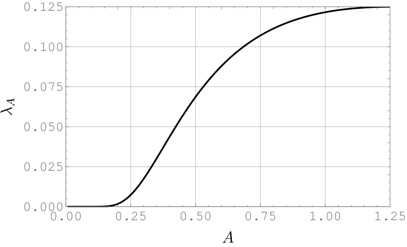
We can now conclude that, if , then the quasi-stationary distribution’s pdf and cdf are given by (30) and (31), respectively, with determined as the only solution of equation (32).
Let us now switch attention to the case when . From the above discussion it follows that this case takes effect for . The quasi-stationary distribution formulae (30) and (31) remain valid “as is”, except that becomes .
At this point we have effectively proved the following two theorems.
Theorem 3.3.
If is the solution of the equation
then for every fixed the equation
has exactly one solution , and the quasi-stationary density is given by
| (34) |
while the respective quasi-stationary cdf is given by
| (35) |
Theorem 3.4.
If is the solution of the equation
then for every fixed the equation
has no solution except attained at , and the quasi-stationary density is given by
| (36) |
while the respective quasi-stationary cdf is given by
| (37) |
Theorems 3.3 and 3.4 both easily follow directly from Lemma 3.1 and the discussion preceding it. It is also worth pointing out that, in view of (28) and (29), formulae (34) and (35) each permit a different expression, similar to that of formulae (36) and (37), respectively. The possibility of formulae (34) and (35) taking the form akin to that of formulae (36) and (37), respectively, is an indication that the quasi-stationary distribution is a smooth, continuous function of .
As complicated as the obtained formulae (34)–(35) and (36)–(37) may seem, they are all perfectly amenable to numerical evaluation, meaning that the quasi-stationary distribution’s pdf and cdf can all be evaluated numerically to within any desired accuracy, for any . To illustrate this point, we implemented the formulae in a Mathematica script, and used it to perform a few numerical experiments each corresponding to a specific value of . The obtained results are presented next.
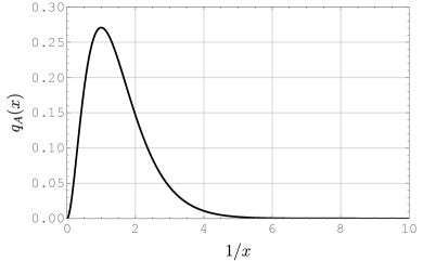
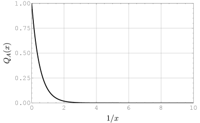
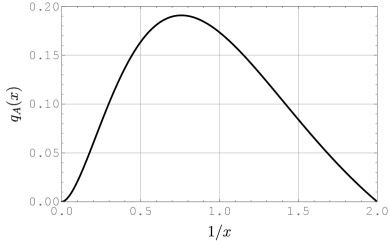
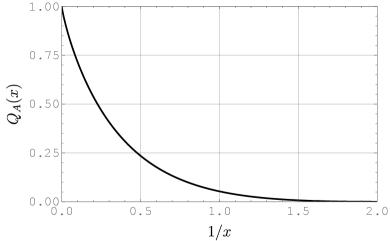
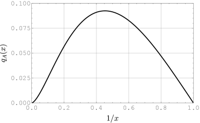
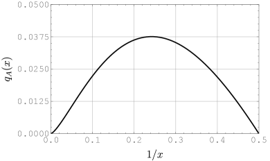
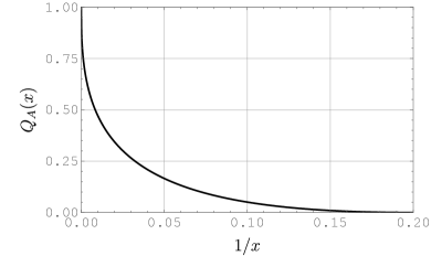
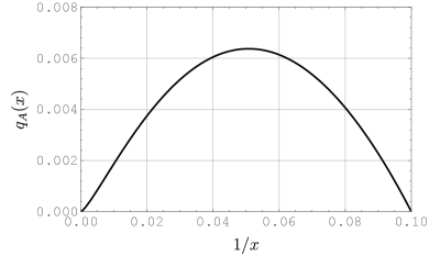
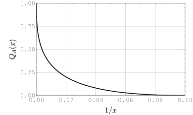
Figures 2, 3, and 4 depict the quasi-stationary pdf and the corresponding cdf as functions of for , , and for , respectively. We stress that the -axis scale is not but is . This is intentional, and is done to achieve finiteness of the domain of the quasi-stationary distribution. On the flip side, however, this transformation effectively reverses the direction of the -axis, which is why the cdf appears as a decreasing function of : it is not, as long as one keeps in mind that the -axis is the reciprocal of . It is also of note that are all smaller than , so that and the corresponding pdf and cdf are given by Theorem 3.3.

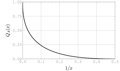
Figures 5, 6, and 7 show the quasi-stationary pdf and cdf for , , and , respectively. Since are all higher than , it follows that and the corresponding pdf and cdf are given by Theorem 3.4.

To draw a line under the entire paper, we remark that formulae (27)–(29) actually give a whole family of quasi-stationary densities indexed by where is the “bottom” of the spectrum of the operator defined in (5). Put another way, for any fixed and any fixed , the function given by formulae (27)–(29) is “legitimate” pdf supported on , because it is nonnegative for any and integrates to unity over the interval . Indeed, first note that if , then must be different from zero for all , for otherwise would not be the smallest eigenvalue. Therefore is either positive or negative for all . To see that cannot be negative, observe that from (31) we have
where we recall that is a constant (independent of but dependent on ) given by either (28) or (29). However, according to (22) and (23), the limit in the right-hand side of the foregoing formula is zero, because whenever , as can be easily seen from (16). Thus given by (27)–(29) integrates to one over the interval . This necessitates that the sign maintained by in the interior of this interval be positive. We therefore arrive at the curious conclusion: formulae (27)–(29) yield a “legitimate” quasi-stationary pdf for any . However, while given (18) is still an eigenfunction of , it satisfies the square-integrability condition only for , i.e., is false, unless . The existence such a continuum of quasi-stationary distributions was also previously predicted in [7, Section 7.8.2]; see also [7, Corollary 6.19, p. 144, and Theorem 6.34, p. 157].
Acknowledgments
The authors would like to thank Dr. E.V. Burnaev of the Kharkevich Institute for Information Transmission Problems, Russian Academy of Sciences, Moscow, Russia, and Prof. A.N. Shiryaev of the Steklov Mathematical Institute, Russian Academy of Sciences, Moscow, Russia, for their interest in and attention to this work.
References
- [1] M. Abramowitz and I. Stegun, eds., Handbook of Mathematical Functions with Formulas, Graphs, and Mathematical Tables, vol. 55 of Applied Mathematics Series, United States National Bureau of Standards, tenth ed., 1964.
- [2] H. Buchholz, The Confluent Hypergeometric Function, vol. 15 of Springer Tracts in Natural Philosophy, Springer-Verlag, New York, NY, 1969. Translated from German into English by H. Lichtblau and K. Wetzel.
- [3] E. V. Burnaev, E. A. Feinberg, and A. N. Shiryaev, On asymptotic optimality of the second order in the minimax quickest detection problem of drift change for Brownian motion, Theory of Probability and Its Applications, 53 (2009), pp. 519–536, https://doi.org/10.1137/S0040585X97983791.
- [4] P. Cattiaux, P. Collet, A. Lambert, S. Martínez, S. Méléard, and J. S. Martín, Quasi-stationary distributions and diffusion models in population dynamics, Annals of Probability, 37 (2009), pp. 1926–1969, https://doi.org/10.1214/09-AOP451.
- [5] E. A. Coddington and N. Levinson, Theory of Ordinary Differential Equations, McGraw-Hill, New York, NY, 1955.
- [6] P. Collet, S. Martínez, and J. S. Martín, Asymptotic laws for one-dimensional diffusions conditioned to nonabsorption, Annals of Probability, 23 (1995), pp. 1300–1314, https://doi.org/10.1214/aop/1176988185.
- [7] P. Collet, S. Martínez, and J. S. Martín, Quasi-Stationary Distributions Markov Chains, Diffusions and Dynamical Systems, Probability and Its Applications, Springer, New York, NY, 2013.
- [8] A. Comtet and C. Monthus, Diffusion in a one-dimensional random medium and hyperbolic Brownian motion, Journal of Physics A: Mathematical and General, 29 (1996), pp. 1331–1345, https://doi.org/10.1088/0305-4470/29/7/006.
- [9] A. De Schepper and M. J. Goovaerts, The GARCH(1,1)-M model: Results for the densities of the variance and the mean, Insurance: Mathematics and Economics, 24 (1999), pp. 83–94, https://doi.org/10.1016/S0167-6687(98)00040-7.
- [10] A. De Schepper, M. Teunen, and M. J. Goovaerts, An analytical inversion of a Laplace transform related to annuities certain, Insurance: Mathematics and Economics, 14 (1994), pp. 33–37, https://doi.org/10.1016/0167-6687(94)00004-2.
- [11] C. Donati-Martin, R. Ghomrasni, and M. Yor, On certain Markov processes attached to exponential functionals of Brownian motion: Application to Asian options, Revista Matemática Iberoamericana, 17 (2001), pp. 179–193, https://doi.org/10.4171/RMI/292.
- [12] D. Dufresne, The integral of geometric Brownian motion, Advances in Applied Probability, 33 (2001), pp. 223–241, https://doi.org/10.1239/aap/999187905.
- [13] N. Dunford and J. T. Schwartz, Linear Operators. Part II: Spectral Theory. Self Adjoint Operators in Hilbert Space, John Wiley & Sons, Inc., New York, NY, 1963.
- [14] E. A. Feinberg and A. N. Shiryaev, Quickest detection of drift change for Brownian motion in generalized Bayesian and minimax settings, Statistics & Decisions, 24 (2006), pp. 445–470, https://doi.org/10.1524/stnd.2006.24.4.445.
- [15] H. Geman and M. Yor, Bessel processes, Asian options, and perpetuities, Mathematical Finance, 3 (1993), pp. 349–375, https://doi.org/10.1111/j.1467-9965.1993.tb00092.x.
- [16] I. S. Gradshteyn and I. M. Ryzhik, Table of Integrals, Series, and Products, Academic Press, eighth ed., 2014.
- [17] K. Itô and H. P. McKean, Jr., Diffusion Processes and Their Sample Paths, Springer, Berlin, Germany, 1974.
- [18] A. Kolmogoroff, Über die analitische Methoden in der Wahrscheinlichkeitsrechnung, Mathematische Annalen, 104 (1931), pp. 415–458, https://doi.org/10.1007/BF01457949. (in German).
- [19] B. M. Levitan, Eigenfunction expansions of second-order differential equations, Gostechizdat Moscow–Leningrad, Leningrad, USSR, 1950. (in Russian).
- [20] B. M. Levitan and I. S. Sargsjan, Introduction to Spectral Theory: Selfadjoint Ordinary Differential Operators, vol. 39 of Translations of Mathematical Monographs, American Mathematical Society, Providence, RI, 1975.
- [21] V. Linetsky, Spectral expansions for Asian (average price) options, Operations Research, 52 (2004), pp. 856–867, https://doi.org/10.1287/opre.1040.0113.
- [22] V. Linetsky, Spectral methods in derivative pricing, vol. 15 of Handbooks in Operations Research and Management Sciences, North–Holland, Netherlands, 2007, ch. 6, pp. 223–299.
- [23] P. Mandl, Spectral theory of semi-groups connected with diffusion processes and its application, Czechoslovak Mathematical Journal, 11 (1961), pp. 558–569.
- [24] S. Martínez and J. S. Martín, Rates of decay and -processes for one dimensional diffusions conditioned on non-absorption, Journal of Theoretical Probability, 14 (2001), pp. 199–212, https://doi.org/10.1023/A:1007881317492.
- [25] S. Martínez and J. S. Martín, Classiffication of killed one-dimensional diffusions, Annals of Probability, 32 (2004), pp. 530–552, https://doi.org/10.1214/aop/1078415844.
- [26] M. A. Milevsky, The present value of a stochasic perpetuity and the Gamma distribution, Insurance: Mathematics and Economics, 20 (1997), pp. 243–250, https://doi.org/10.1016/S0167-6687(97)00013-9.
- [27] C. Monthus and A. Comtet, On the flux distribution in a one dimensional disordered system, Journal de Physique I: France, 4 (1994), pp. 635–653, https://doi.org/10.1051/jp1:1994167.
- [28] G. Peskir, On the fundamental solution of the Kolmogorov–Shiryaev equation, in From Stochastic Calculus to Mathematical Finance: The Shiryaev Festschrift, Y. Kabanov, R. Liptser, and J. Stoyanov, eds., Springer, Berlin, 2006, pp. 535–546, https://doi.org/10.1007/978-3-540-30788-4_26.
- [29] M. Pollak and D. Siegmund, A diffusion process and its applications to detecting a change in the drift of Brownian motion, Biometrika, 72 (1985), pp. 267–280, https://doi.org/10.1093/biomet/72.2.267.
- [30] A. S. Polunchenko, Asymptotic near-minimaxity of the randomized Shiryaev–Roberts–Pollak change-point detection procedure in continuous time, Theory of Probability and Its Applications, 64 (2017), pp. 769–786, https://doi.org/10.4213/tvp5142.
- [31] A. S. Polunchenko, On the quasi-stationary distribution of the Shiryaev–Roberts diffusion, Sequential Analysis, 36 (2017), pp. 126–149, https://doi.org/10.1080/07474946.2016.1275512.
- [32] A. S. Polunchenko and G. Sokolov, An analytic expression for the distribution of the generalized Shiryaev–Roberts diffusion: The Fourier spectral expansion approach, Methodology and Computing in Applied Probability, 18 (2016), pp. 1153–1195, https://doi.org/10.1007/s11009-016-9478-7.
- [33] M. Schröder, On the integral of geometric Brownian motion, Advances in Applied Probability, 35 (2003), pp. 159–183, https://doi.org/10.1239/aap/1046366104.
- [34] A. N. Shiryaev, The problem of the most rapid detection of a disturbance in a stationary process, Soviet Mathematics—Doklady, 2 (1961), pp. 795–799. (Translated from Dokl. Akad. Nauk SSSR 138:1039–1042, 1961).
- [35] A. N. Shiryaev, On optimum methods in quickest detection problems, Theory of Probability and Its Applications, 8 (1963), pp. 22–46, https://doi.org/10.1137/1108002.
- [36] A. N. Shiryaev, Quickest detection problems in the technical analysis of the financial data, in Mathematical Finance—Bachelier Congress 2000, H. Geman, D. Madan, S. R. Pliska, and T. Vorst, eds., Springer Finance, Springer, Berlin, 2002, pp. 487–521, https://doi.org/10.1007/978-3-662-12429-1_22.
- [37] L. J. Slater, Confluent Hypergeometric Functions, Cambridge University Press, Cambirdge, UK, 1960.
- [38] E. C. Titchmarsh, Eigenfunction Expansions Associated with Second-Order Differential Equations, Clarendon, Oxford, UK, 1962.
- [39] M. Vanneste, M. J. Goovaerts, and E. Labie, The distribution of annuities, Insurance: Mathematics and Economics, 15 (1994), pp. 37–48, https://doi.org/10.1016/0003-4916(88)90283-7.
- [40] E. T. Whittaker, An expression of certain known functions as generalized hypergeometric functions, Bulletin of the American Mathematical Society, 10 (1904), pp. 125–134.
- [41] E. T. Whittaker and G. N. Watson, A Course of Modern Analysis, Cambridge University Press, fourth ed., 1927.
- [42] E. Wong, The construction of a class of stationary Markoff processes, in Stochastic Processes in Mathematical Physics and Engineering, R. Bellman, ed., American Mathematical Society, Providence, RI, 1964, pp. 264–276.
- [43] M. Yor, On some exponential functionals of Brownian motion, Advances in Applied Probability, 24 (1992), pp. 509–531.