A unified decision making framework for supply and demand management in microgrid networks

Abstract

This paper considers two important problems - on the supply-side and demand-side respectively and studies both in a unified framework. On the supply side, we study the problem of energy sharing among microgrids with the goal of maximizing profit obtained from selling power while at the same time not deviating much from the customer demand. On the other hand, under shortage of power, this problem becomes one of deciding the amount of power to be bought with dynamically varying prices. On the demand side, we consider the problem of optimally scheduling the time-adjustable demand - i.e., of loads with flexible time windows in which they can be scheduled. While previous works have treated these two problems in isolation, we combine these problems together and provide a unified Markov decision process (MDP) framework for these problems. We then apply the Q-learning algorithm, a popular model-free reinforcement learning technique, to obtain the optimal policy. Through simulations, we show that the policy obtained by solving our MDP model provides more profit to the microgrids.

I Introduction

A microgrid is a networked group of distributed energy sources with the goal of generating, converting and storing energy. While the main power stations are highly connected, microgrids with local power generation, storage and conversion capabilities, act locally or share power with a few neighboring microgrid nodes [1]. This scenario is being envisaged as an important alternative to the conventional scheme with large power stations transmitting energy over long distances.

In order to take full advantage of the modularity and flexibility of microgrid technologies, smart control mechanisms are required to manage and coordinate these distributed energy systems so as to minimize the costs of energy production, conversion and storage, without jeopardizing the central smart grid stability. Augmenting microgrid with smart controls however involves addressing many problems. In this paper, we address two problems. (i) Supply-side management (SSM) problem: energy sharing among microgrids under stochastic supply and demand along with optimal battery scheduling of each microgrid and (ii) Demand-side management (DSM) problem: efficiently scheduling the time adjustable demand from smart appliances in a smart home environment along with non-adjustable demand. Our goal here is to maximize profit earned by microgrids from selling excess energy while maintaining a low gap between demand and supply. We address these learning and scheduling problems by modeling them in the framework of Markov decision process (MDP) [2].

A simple example which explains the specific problem that we are trying to solve on the supply side using our proposed framework is the following. Consider three microgrids MG-1, MG-2, and MG-3 with their respective forecasted demand and supply profiles over two time intervals as in Table I. Here, supply denotes the power available to the microgrid from its renewable energy sources (though, accurate prediction of the supply from renewable energy sources is a challenge). Let us assume for this example, that the microgrids do not buy power from the central main grid to which they are connected. Let the price of the power (per unit) in time interval 2 be higher than the price in time interval 1 (this information is not known to the microgrids a priori). Below are three possible power sharing scenarios, between these microgrids.

Table I: Sample forecasted demand & supply profiles

Microgrid #	Interval 1		Interval 2
	demand	supply	demand	supply
MG-1	1	2	1	0
MG-2	1	0	1	1
MG-3	1	2	1	1

1. Power sharing is not allowed between microgrids. Then there is power deficiency in microgrid MG-2 during the time interval 1 and in the microgrid MG-1 during the time interval 2.

2. Power sharing is allowed between microgrids, MG-2 buys power from MG-1 in interval 1, MG-3 stores it’s excess power in the battery in interval 1, and MG-1 buys power from MG-3 in interval 2.

3. Power sharing is allowed between microgrids, MG-2 buys power from MG-3 in interval 1, and MG-1 stores it’s excess power in the battery in interval 1 for consumption in interval 2.

Scenario 2 addresses the power deficiency issue in Scenario 1. However a more intelligent way of handling the power deficiency for MG-1 is possible in Scenario 3. In the Scenario 2, the profit obtained by MG-1 (which is negative as it sells the power when the price is low and buys it when the price is high) is less than the profit obtained by it in the Scenario 3 (which is zero). Our objective, therefore in this framework, is to obtain an optimal power buying and selling policy for microgrids, so as to maximize the overall profits , in the presence of renewable energy supply sources and dynamically varying power prices.

An assumption we make in this work is that, in any microgrid, when supply meets the demand in a given interval, it is to be understood that the demand represents the actual power consumption by the consumers, plus the electric power transmission and distribution losses. We however do not explicitly try to minimize the power transmission and distribution losses. Our framework inherently tries to minimize these power losses, by drawing power preferably from nearby peer microgrids as opposed to far-away microgrids.

I-A Supply-side management (SSM) problem

Cooperative energy exchange among microgrids is a popular technique in SSM for efficient energy distribution. Local energy sharing/exchange between microgrids has the following advantages: (a) it can significantly reduce power wastage that would otherwise result over long-distance transmission lines, and (b) it helps satisfy demand and reduce reliance on the main/central grid. Figure 1 shows a cooperative energy exchange model with multiple microgrids (on the distribution side of the network) that can cater to their individual local loads. Each microgrid controls its local sub-network through its controller (labeled $\mbox{C}_{1}$, $\mbox{C}_{2}$ etc.) that mainly has access to its local state information.

Figure 1: Cooperative Energy Exchange Model

In classical power grids, system level optimization is done based on a centralized objective function, where as a microgrid network has heterogeneous nature right from the manner in which electricity is generated such as from wind turbines, solar farms and diesel generators to energy storage devices such as batteries and capacitors. Because of this heterogeneity and the fact that energy can be shared between microgrids depending on requirements, one needs to consider distributed techniques to control and optimize a smart grid system with a distribution network catering to multiple microgrids.

Related work : The literature considering the energy exchange among the microgrids is vast. A survey on game theoretic approaches for microgrids is considered in [3]. This survey examines both cooperative energy sharing models as well as non-cooperative game models for distributed control of microgrids assuming that the system model is known. Energy sharing among the microgirds is studied in [4] with the objective of minimizing the energy bills for the microgrids. This work is later extended in [5] to consider the price-based demand response. [6, 7, 8] and [9] consider multi-agent systems for energy trading and control of microgrids under various objectives and formulations. However, most of the existing literature assumes that the underlying distributions for both supply and demand are known. But this doesn’t hold good especially in the context of microgrids with renewable energy sources as there is significant randomness in the amount of energy generated. Since models for energy dynamics are very unreliable [10] due to randomness at various stages, one needs to use model-free and data-driven algorithms to address these problems. Because of their model-free nature, Reinforcement Learning (RL) [11] approaches that are primarily data-driven control techniques play a significant role in solving these problems. The first step in this direction is to formulate the problem in the Markov Decision Process (MDP) framework. In section II, we provide the details of our proposed model for the energy trading problem among the microgrids in order to maximize profits, adhering to the average-cost MDP framework [12].

I-B Demand-side management (DSM) problem

Load shifting is a popular technique used in demand-side management (DSM) [13]. It involves moving the consumption of load to different times within an hour, a day, or a week. It does not result in reduction in the net quantity of energy consumed, but simply involves changing the time when the energy is consumed. Load shifting facilitates the customer in reducing the energy consumption cost and at the same time it helps the smart grid in managing the peak load.

With increased use of smart appliances and smart home environments, the concept of load shifting is becoming increasingly popular for the smart grid as the demand from smart appliances is time adjustable in general. One or more of these smart appliances collectively achieve some activity in the smart home environment, called ADL (activity of daily living). It is possible to monitor and identify the ADLs in smart home environments [14]. With the help of smart home technology, it is possible to find the amount of load each ADL puts on the grid, and also the allowed time window during which the ADL would perform the activity (e.g., scheduling a washing machine for an hour to clean the clothes anytime between 3PM to 6PM). The demand from ADLs need not be met during a fixed time period, instead it could be met during any time period within a flexible time window. With the help of the advanced metering infrastructure (AMI) that provides a two-way communication between the utility and customers, it is possible to make a decision on when to schedule the ADL demand at the smart grid and convey the same to the customer’s smart meter.

There is regular demand that needs to be met at fixed time periods, apart from the ADL related demand associated with any customer. This regular demand of a smart home will be called non-ADL demand in the rest of the paper. Similarly, the demand from ADL of the smart home will be called ADL demand.

There is prior work around scheduling the ADL-demand using the load shifting technique for handling peak load scenarios [15]. However, the authors make the unrealistic assumption of precisely knowing the supply profile while doing such a scheduling of the ADL-demand. In this paper, we propose scheduling of ADL-demand using the load shifting technique with uncertainty in the supply profile generated (e.g., renewable energy sources like solar or wind being the primary sources of power generation).

Our main contributions:
(i) To the best of our knowledge, we are the first to integrate both the demand-side and supply-side management problems of a network of microgrids in a unified Markov decision process framework. We apply Reinforcement Learning (RL) algorithms which do not require knowledge of the underlying system model to address these problems. Our algorithms are easy to implement.
(ii) We perform for the first time, optimal scheduling of ADL demand when both demand and power generation are stochastic in nature. Even though this is the most natural scenario, it had not been studied previously.
The rest of the paper is organized as follows. In section II, we discuss in detail about the problem formulation using the MDP framework. We present in section III the Q-learning algorithm. In section IV, we present simulation experiments along with other algorithms for comparison. Finally, in section V, we provide the concluding remarks.

II Problem formulation and the mdp model

We consider $N$ microgrids denoted by $1,\ldots,N$ which are inter-connected through the central electric grid distribution network. Each microgrid comprises of the distributed small scale renewable power generation sources that are equipped with energy storage devices. We divide a day into $t$ time units during which the decisions about power allocation are made. At every time instant $t$ of a day, the $i^{th}$ microgrid controller $C_{i}$ has access to the following information:

1. Total renewable energy ($r_{t}^{i}$) generated from it’s energy sources.

2. Price per unit energy ($p_{t}$) decided by the main grid
   at time $t$.

3. Accumulated non-ADL demand ($d_{t}^{i}$) from each load.

4. Set of all ADL jobs ($J_{t}^{i}$). $J_{t}^{i}$ has the form $\{\gamma_{1}^{i},\ldots,\gamma_{n}^{i}\}$, where the $j^{th}$ ADL job $\gamma_{j}^{i}=(a_{j}^{i},f_{j}^{i})$. Here, $a_{j}^{i}$ represents the number of units of energy required to finish the job, and $f_{j}^{i}$ represents the number of future time instants remaining (after the current time instant $t$) by when the controller $C_{i}$ can schedule the job $\gamma_{j}^{i}$ without incurring a penalty.

5. Let $B_{i}$ represent the maximum battery capacity of the microgrid $i$ and $b_{t}^{i}$ the amount of power available in the battery at time $t$. Here $0\leq b_{t}^{i}\leq B_{i}$ for any time instant $t$.

From the above available information, microgrid controller $C_{i}$ at every time step $t$ has to decide on the following choices:

1. Amount of energy it needs to buy (sell) from (to) the main grid.

2. Amount of energy it needs to buy (sell) from (to) the neighboring microgrids.

3. Amount of energy it needs to store (retrieve) into (from) its storage device.

4. The subset of ADL jobs it needs to schedule.

Both the demand and energy generated at each microgrid are uncertain due to the random nature of loads ($d_{t}^{i}$ and $J_{t}^{i}$) and the amount of renewable energy generation ($r_{t}^{i}$) in time slot $t$. Therefore, this problem falls in the realm of Markov Decision Process (MDP). In the next subsection we provide the details of our MDP model.

Figure 2: Actions of an RL agent at each time instant $t$

II-A MDP framework

MDP is a general framework for modeling problems of dynamic optimal decision making under uncertainty. An MDP is a tuple $<\mathcal{S},\mathcal{U},\mathcal{R},\mathcal{P}>$, where $\mathcal{S}$ is the set of all states, $\mathcal{U}$ is the set of feasible actions, $\mathcal{R}:\mathcal{S}\times\mathcal{U}\times\mathcal{S}\to\mathbb{R}$ is the single- stage reward function and $\mathcal{P}$ is the state transition probability matrix. In RL, an agent interacts with the environment by observing state $s_{t}\in\mathcal{S}$ and picking an action $u_{t}\in\mathcal{U}$. The new state $s_{t+1}$ is obtained from the state transition probability $\mathcal{P}(s_{t+1}|s_{t},u_{t})$ and yields a reward $g_{t}=\mathcal{R}(s_{t},u_{t},s_{t+1})$. The goal of the RL agent is to learn the optimal sequence $\{u_{t}\}$ of actions so as to maximize its average expected return (see Section II-B).

We begin by specifying the states, actions and single-stage rewards, for our MDP model.

II-A1 State space

The state $s_{t}^{i}$ at time instant $t$ for the microgrid $i$ is the following tuple:

$$s_{t}^{i}=(t,nd_{t}^{i},p_{t},J_{t}^{i}),$$ (1)

where the net demand $nd_{t}^{i}=r_{t}^{i}+b_{t}^{i}-d_{t}^{i}$. If $nd_{t}^{i}>0$, then there is excess of power after meeting the non-ADL demand and if $nd_{t}^{i}<0$, there is a deficit in power even to meet the non-ADL demand. The state also includes time $t$ since optimal action can depend on it. For example, a microgrid operating on solar renewable generation can sell excess power during the morning as the solar power will be available even during afternoon. But it may not be a good choice to aggressively sell it in the evening as there will be no solar power generation during the night.

II-A2 Action space

Let $P_{t}^{i}$ be the power set of $J_{t}^{i}$, which consists of all possible combinations of the ADL jobs that can be scheduled at time instant $t$ at microgrid $i$. We define another set $A_{t}^{i}$, that denotes the total aggregated ADL demand for each element in $P_{t}^{i}$. For example, the $j^{th}$ element $A_{t}^{i}(j)=\sum_{k=1,\gamma_{k}^{i}\in P_{t}^{i}(j)}^{n}a_{k}^{i}$, where $P_{t}^{i}(j)$ is the $j^{th}$ element in $P_{t}^{i}$ and $n$ is the total number of elements in $P_{t}^{i}(j)$.

At each time instant $t$, the microgrid controller needs to make two decisions $u_{t}^{i}$ and $v_{t}^{i}$.

• When $u_{t}^{i}$ is negative, $|u_{t}^{i}|$ represents the amount of power drawn from the peer microgrids/maingrid to meet the non-ADL demand along with optionally storing in the battery (if the power is bought, it is first used to meet the non-ADL demand).

• When $u_{t}^{i}$ is positive, $|u_{t}^{i}|$ represents the amount of power sold to the peer microgrids/maingrid from the battery storage and energy generated from renewable sources.

• The second action $v_{t}^{i}$ pertains to the scheduling decision of ADL jobs taken by microgrid controller $C_{i}$. $v_{t}^{i}$ is always non-positive, and $|v_{t}^{i}|$ represents the power needed to meet the ADL demand in time interval $t$ at microgrid $i$. Formally, if the $j^{th}$ element of the set $P_{t}^{i}$ is selected at time $t$, $|v_{t}^{i}|$ is equal to $A_{t}^{i}(j)$.

The feasible region for the action $u_{t}^{i}$ is as follows:

$$-min(M,B_{i}-nd_{t}^{i}+ \max_{1\leq j\leq 2^{n}}A_{t}^{i}(j))\leq u_{t}^{i}+v_{t}^{i}$$

$$\leq max(0,nd_{t}^{i}),$$ (2)

where $M$ denotes the maximum amount of power a microgrid can buy to meet the demand. This constraint is to maintain the stability of the main grid. The above bounds indicate that the microgrid can sell the surplus; or can buy energy to meet the non-ADL demand, ADL demand and to fill its battery. Note that there is flexibility for microgrids to buy (sell) this power from (to) the neighboring microgrids. If it needs to buy (sell) more power, only then it buys (sells) it from (to) the main grid. In this way, we allow for cooperation among the microgrids. Further this makes sure that the demand at the main grid is controlled at all the times.

Let $\widehat{J}_{t+1}^{i}$ be the new set of ADL jobs received by the microgrid $i$ in the time interval $t+1$. Depending on the action $v_{t}^{i}$, not all the ADL jobs might have got scheduled in the time interval $t$. The ADL jobs which are not scheduled in the time interval $t$ but are eligible to be scheduled beyond time interval $t$ are considered in the time interval $t+1$ along with the new jobs $\widehat{J}_{t+1}^{i}$. Thus, we have $J_{t+1}^{i}=\widehat{J}_{t+1}^{i}\cup\widetilde{J}_{t}^{i}$, where $\widetilde{J}_{t}^{i}=\{\,(a_{j}^{i},f_{j}^{i}-1)\,\,|\,\,(a_{j}^{i},f_{j}^{i})\in\overline{J}_{t}^{i}\,\,and\,\,f_{j}^{i}>0\,\}$ and $\overline{J}_{t}^{i}=J_{t}^{i}-P_{t}^{i}$.

The battery information is updated as follows:

$$b_{t+1}^{i}=max(0,nd_{t}^{i}-u_{t}^{i}),$$ (3)

which denotes the power available after meeting the non-ADL demand. Figure 2 illustrates the actions of a microgrid at every time instant $t$.

II-A3 Single-stage reward function

We want to maximize the profit of each microgrid obtained by selling power while reducing the demand and supply deficit. Our single-stage reward function has components for both the reward obtained by selling power and penalty for unmet demand. The single-stage reward function for the microgrid $i$ at time $t$ is as follows:

$$g^{i}(s_{t}^{i},u_{t}^{i},v_{t}^{i})= p_{t}*(u_{t}^{i}+v_{t}^{i})+c*min(0,nd_{t}^{i}-u_{t}^{i})$$

$$-c*\sum_{k=1}^{n}I_{\{f_{k}^{i}=0\}}a_{k}^{i}.$$ (4)

The first term in (II-A3) represents the loss/gain incurred for buying/selling power while the second and third terms represent the penalty incurred for not meeting the non-ADL and the ADL demands respectively. Here, $c\,\,(\geq 0)$ is the penalty per unit of unmet demand and $I_{\{f_{k}^{i}=0\}}$ is the indicator random variable which equals one if $f_{k}^{i}=0$ and is zero otherwise. Here $c$ acts as a threshold between the profit of the microgrid and the penalty for not satisfying the demand. For example, when $c=0$, each microgrid takes decision to maximize its profit without satisfying any customer demand. On the other hand, if the value of $c$ is very high, microgrids need to satisfy customer demand at every time instant as they incur huge penalty otherwise. Next, we provide the long-run average cost objective function.

II-B Average cost setting

The objective is to maximize the expected average profit obtained by all the microgrids. The long-run average profit objective function $J^{i}(\pi)$ of the microgrid $i$ for a given policy $\pi$ is given as follows:

$$J^{i}(\pi):=\lim\sup_{n\rightarrow\infty}\frac{1}{n}\,\,\mathbb{E}\left(\left.\sum_{t=0}^{n}g^{i}(s_{t},u_{t},v_{t})\right|\pi\right),$$ (5)

where $E(.)$ denotes the expected value. Here we view a policy $\pi$ as the map $\pi:S\to A$ which assigns for any state $s$, a certain feasible action $a$. The goal of our RL agent $i$ is to find $\pi_{i}^{*}=\mathop{\rm arg\,max}_{\pi\in\Pi}J^{i}(\pi)$, where $\Pi$ is the set of all feasible policies.

III Algorithm

In this work, we do not assume any model of the system (i.e., probability transition model of the demand, supply as well as renewable energy generation). We apply Reinforcement Learning algorithms that do not assume any model of the environment to provide optimal solution. We assume that we have access to a simulator that provides the state samples (i.e., Non-ADL and ADL demand, price) at every time instant to the algorithm. This can be achieved, for instance, through smart meters deployed in households. We employ the Average-Cost Q-Learning algorithm, a popular RL method for solving the average cost problem in section II-B. We apply the Relative Value Iteration (RVI) based Q-Learning algorithm for each agent $i$, proposed in [12]. The algorithm is described below.

Let $Q_{t}^{i}(s^{i}_{t},u^{i}_{t})$ represent the Q-value estimate corresponding to state $s^{i}_{t}$ and action $u^{i}_{t}$ for the agent $i$ in the $t^{th}$ iteration. The initial Q-values associated with all states and actions are set to zero i.e., $Q_{0}^{i}(s^{i},u^{i})=0$ $\forall\hskip 2.84544pt(s,u)$ and $\forall i$. Subsequently, the Q-values are updated as follows (using similar notations as in [12]):

$$Q^{i}_{t+1}(s^{i}_{t},u^{i}_{t}) =Q^{i}_{t}(s^{i}_{t},u^{i}_{t})+\alpha(t,s^{i},u^{i})(g^{i}(s^{i}_{t},u^{i}_{t},s^{i}_{t+1})+$$

$$max_{u}Q^{i}_{t}(s^{i}_{t+1},u)-f(Q^{i}_{t})-Q^{i}_{t}(s^{i}_{t},u^{i}_{t})),$$ (6)

where $\alpha(.)$ is the learning rate, $g^{i}(s^{i}_{t},u^{i}_{t},s^{i}_{t+1})$ is the reward obtained by taking an action $u^{i}_{t}$ in state $s^{i}_{t}$ and transitioning to the state $s^{i}_{t+1}$ and $f(Q^{i}_{t})$ is a Lipschitz continuous function satisfying suitable conditions specified in [12]. This term is subtracted from (III) to maintain stability of the update equation. It is shown in [12] that $f(Q^{i}_{t})$ converges to the optimal average cost as $t\rightarrow\infty$. One such function $f(.)$ that satisfies the conditions is $max_{u}Q^{i}_{t}(s^{{}^{\prime}},u)$, where $s^{{}^{\prime}}$ is an arbitrarily chosen, fixed state. Therefore the final update equation for the Q-values for each agent $i$ is as follows:

$$Q^{i}_{t+1}(s^{i}_{t},u^{i}_{t}) =Q^{i}_{t+1}(s^{i}_{t},u^{i}_{t})+\alpha(t,s^{i},u^{i})(g^{i}(s^{i}_{t},u^{i}_{t},s^{i}_{t+1})+$$

$$max_{u}Q^{i}_{t}(s^{i}_{t+1},u)-max_{u}Q^{i}_{t}(s^{{}^{\prime}},u)-Q^{i}_{t}(s^{i}_{t},u^{i}_{t})),$$ (7)

At each iteration of this algorithm, the agent $i$ selects an action $u^{i}_{t}$ for the current state $s^{i}_{t}$ using the $\epsilon-$greedy policy. That is, a random action is selected with probability $\epsilon$ and the action that maximizes the current Q-estimate is selected with probability $1-\epsilon$. The simulator takes the current $(s^{i}_{t},u^{i}_{t})$ pair and generates the current stage reward and the next state. In [12], it is shown that under an appropriate learning rate, the algorithm converges to the optimal Q-values which implicitly give the optimal policy. Each microgrid runs a version of this algorithm independently until convergence. The optimal policy of microgrid $i$ is obtained as follows:

$$\pi_{i}^{*}(s)=\mathop{\rm arg\,max}_{u}Q_{*}^{i}(s,u)$$ (8)

that is, the optimal action in state $s$ is obtained by taking the maximum over all actions of the Q-values in state $s$.

IV Simulation Experiments

We implement our model on networks with three and five microgrids, respectively. In the three microgrid setup, two of the microgrids have solar renewable energy as the power supply source while the third operates on wind energy. In the five microgrid network, two of the microgrids use solar renewable energy as the power supply source, two of them use wind renewable energy as the power supply source and one does not have any access to renewable energy. To simulate the renewable generation, we use the RAPsim software [16]. RAPsim is an open source simulator for analyzing the power flow in microgrids. It has a provision for simulating the renewable generation, which is the main feature that we use in our experiments.

IV-A Implementation

We solve the MDP model described in section II and refer to it as the ADL-sharing model. For comparison purposes, we also solve the following MDP models.

• Greedy-ADL model: In this model, microgrids exhibit greedy behavior. They share power only after filling their respective batteries fully. The actions $u_{t}^{i}$ and $v_{t}^{i}$ at each time instant $t$ are bounded as follows:

  $$-min(M, B_{i}-nd_{t}^{i}+\max_{1\leq j\leq 2^{n}}A_{t}^{i}(j))\leq u_{t}^{i}+v_{t}^{i}$$

  $$\leq max(0,nd_{t}^{i}-B_{i}).$$ (9)

  Thus, if $nd_{t}^{i}<0$, decision is taken on the amount of power to buy in order to satisfy the demand and to fill the battery. If $nd_{t}^{i}>0$, then the generated excess power by the microgrid $i$ in time interval $t$ is first used to fill the battery fully and if more power is left, it will be sold to the other microgrids/main grid.

• Non-ADL model: In this model, ADL demand is treated as normal demand. Penalty is levied immediately if the demand is not met in the current time slot.

IV-B Simulation setup

We used the RAPsim simulator to generate per hour renewable energy data for each of the microgrids. We used this data to fit a Poisson distribution for energy generation at each microgrid. We limit the maximum renewable energy available at each time instant to 8 units. The number of decision time intervals in a day is taken to be 4.

For each time period, non-ADL demand ($d_{t}^{i}$) at each of the microgrids can be one of the following three values: 2, 4 or 6 units. The price ($p_{t}^{i}$) per unit energy value (in USD) is considered to be one of 5, 10 or 15. The transition probability matrix for non-ADL demand and the price values are generated randomly.

For our experiments, the maximum size of the battery ($B_{i}$) is set to 8 units and the maximum power that a microgrid can obtain from the main grid ($M$) is limited to 14 units. At each microgrid, we consider 3 ADL jobs, $\{\gamma_{1}^{i}=(1,2),\gamma_{2}^{i}=(1,3),\gamma_{3}^{i}=(2,4)\}$ at the start of the day, where ADL job $\gamma_{j}^{i}=(a,b)$ requires $a$ units of demand within $b\,\,(>0)$ time slots. In the $Non-ADL$ model, the ADL demand is added to the demand at $t=1$ each day. We ran all our simulations for each of the following $c$ (penalty in USD per unit of unmet demand) values : 0, 5, 10 and 30, respectively.

IV-C Results

The algorithms are trained for $10^{7}$ cycles. We used the average profit obtained by each microgrid as a performance metric to evaluate the models.

Figures  3 and  5 plot the average profit obtained for each microgrid in the two settings of three and five microgrid networks, respectively, versus the number of iterations, when $c=0$ in each case. We can see that the algorithms show convergence as the number of iterations increase.

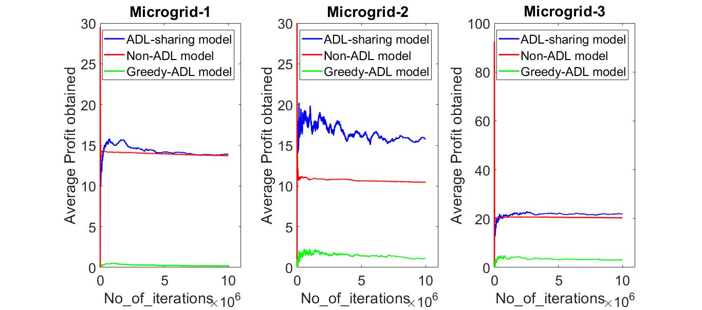
Figure 3: Convergence of algorithms for the three models when $c=0$ for the three microgrid network as a function of number of iterations.

Figures  4 and  6 on the other hand plot the average profit obtained for each microgrid versus $c$ (i.e., penalty per each unit of unmet demand) for all the three models. We run the trained models for 1000 runs to obtain the average profit in each case.

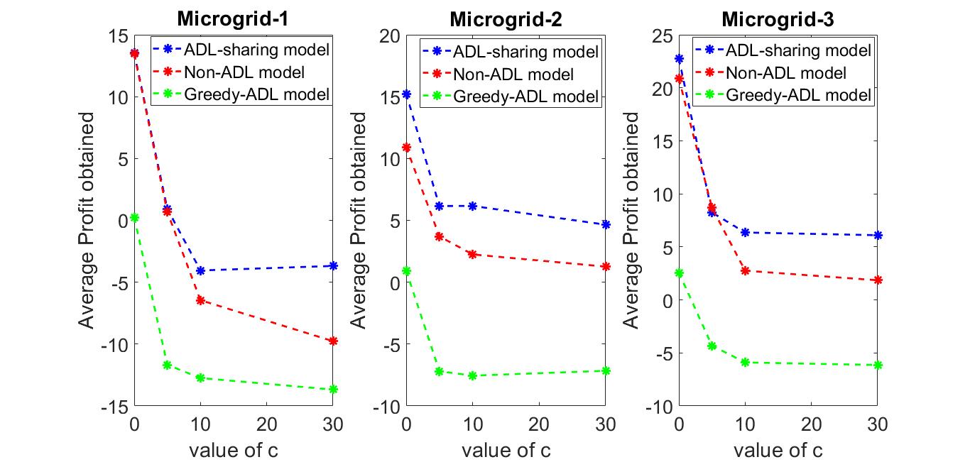
Figure 4: Performance Comparisons of the three models on each microgrid in the three microgrid network as a function of $c$.

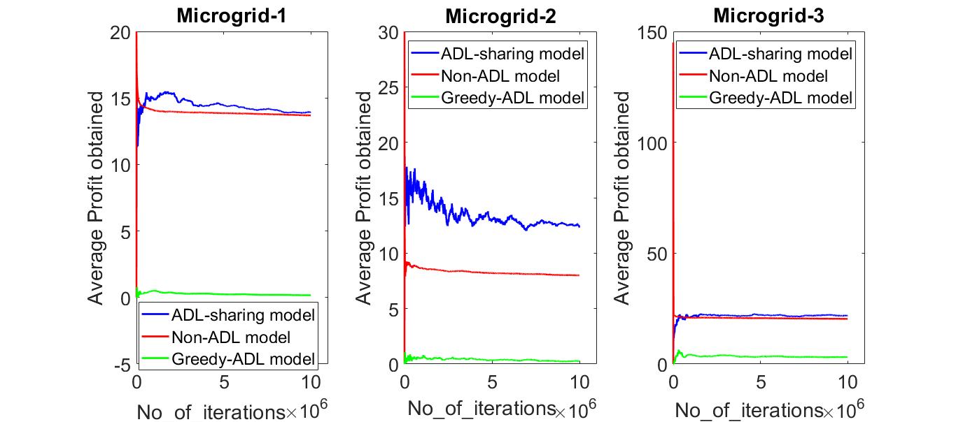
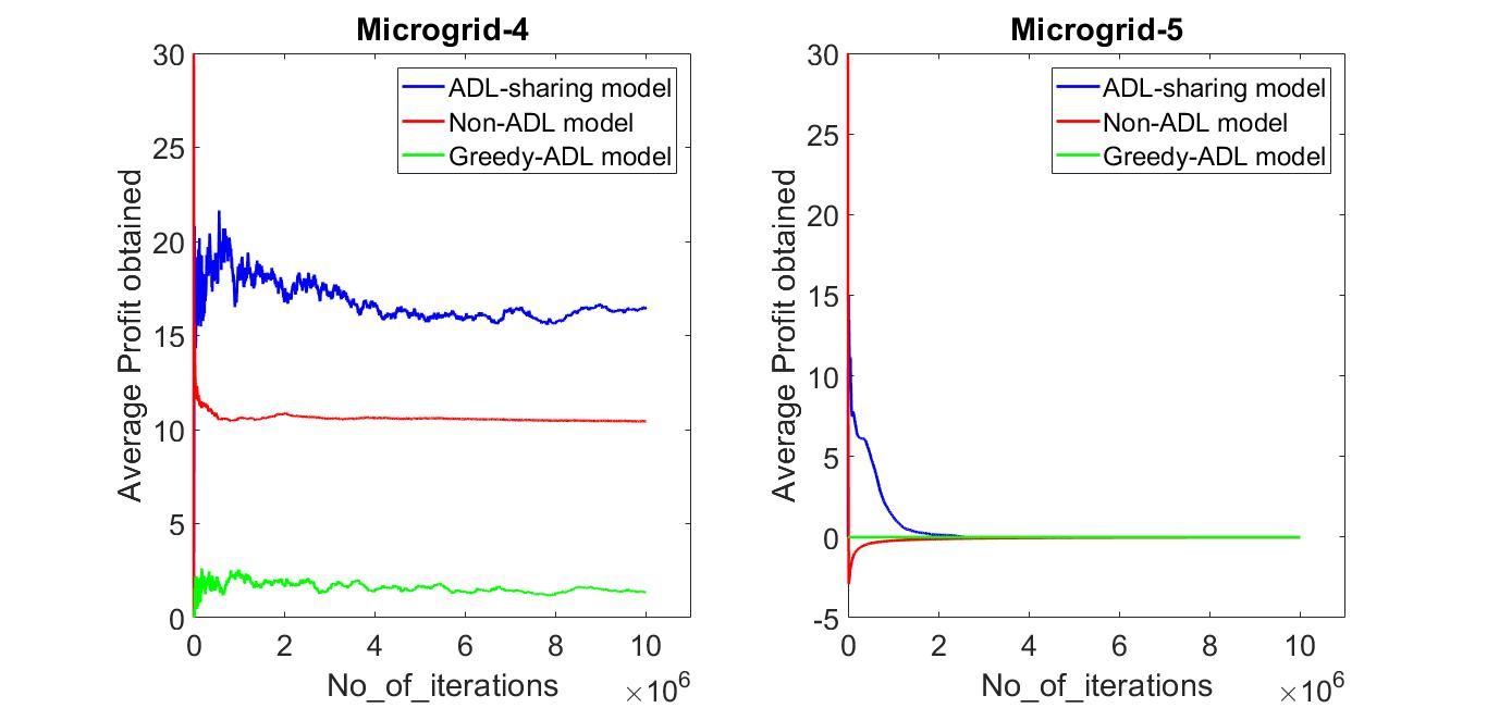
Figure 5: Convergence of algorithms for the three models when $c=0$ for the five microgrid network as a function of number of iterations.

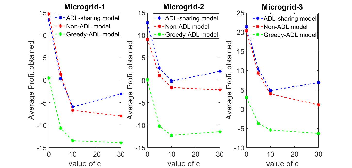
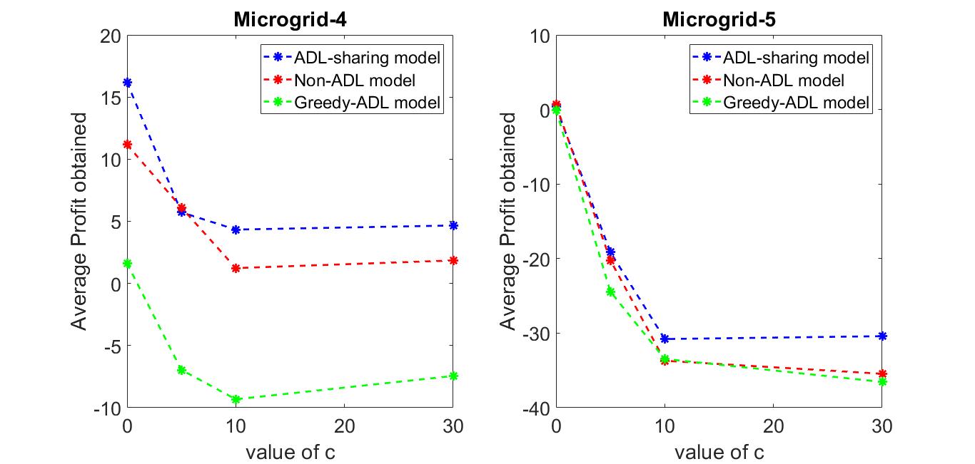
Figure 6: Performance Comparisons of the three models on each microgrid in the five microgrid network as a function of $c$.

IV-D Discussion

From our experiments we make the following observations:

• When $c=0$, the microgrid controllers need not buy power to satisfy the excess demand as they do not incur penalty for not meeting the demand. In the $ADL-sharing$ and $Non-ADL$ models, we observe that all the controllers fill the battery when the price is low while they sell power when the price is high. Hence, the profit obtained is very high compared to the $Greedy-ADL$ model where the power is bought to first fill the battery.

• As the value of $c$ increases, we expect that the profit earned by the microgrid would decrease. This is because the penalty for not meeting the demand would increase. From Figure  6, we observe that profit for $c=30$ is slightly higher than when compared with the case of $c=10$ for $ADL-Sharing$ model. This is due to the high variance in the solar generation during the testing phase. When the value of $c$ is set to 30, the demand at all times will be met without any penalty.

• We observe that the profit gap between the $ADL-sharing$ method and the $Non-ADL$ method increases as the value of $c$ increases. This shows that the profit of the microgrids increases due to the flexibility available to the controllers in scheduling the demand by following the $ADL-sharing$ model.

• The sharing among the microgrids happens as follows: A microgrid operating on solar renewable energy source in the second time period shares the excess power with the other microgrids, as it generates more power as the day progresses. At the same time, a microgrid operating on wind renewable energy source buys power to store in its battery, if it expects more demand than the power it generates in future time periods.

From the above discussion we conclude that our proposed $ADL-sharing$ model provides more profits by exhibiting the following intelligent behavior:

1. Schedules few of the ADL jobs at the beginning, few at the end and few in the middle of their allowed execution time window to exploit flexible nature of the ADL demand.

2. Microgrids do not sell all of their surplus energy to the other microgrids if there is more demand than supply in the future (particularly, solar microgrids sell excess energy during the midday but not at the end of the day).

V Conclusion

Providing a unified solution framework for modeling both demand-side management problem (scheduling ADL jobs) and supply-side management problem (enabling cooperative energy exchange among the microgrids) is a challenging task, particularly when both demand and supply are considered stochastic. We have studied these two problems, for the first time, in a unified framework by using MDPs. Also, for the first time in the literature, we proposed the method of scheduling ADL demand at the microgrid level as a load shifting technique. RL algorithms provide an optimal solution methodology for solving MDP when the underlying model is not known. We apply the Q-learning algorithm to maximize the profit earned by microgrids by selling excess energy while maintaining a low gap between demand and supply. Based on the simulation experiments, we show that the policy obtained by our MDP model (ADL-sharing model) consistently outperforms the policies obtained by other models.

As future work, we would like to consider the pricing mechanism for microgrids. In the current model, the transaction of power is carried out at the price decided by the main grid. The pricing mechanism allows microgrids to bid for the selling price as well as buying price. One can use RL agents to bid for adaptive prices in such a way that microgrids maximize their profits. Another important future work is to use RL algorithms with function approximation to scale the proposed algorithms. The challenge here is to select the appropriate features to obtain an optimal policy.

References

- [1] H. Farhangi, “The path of the smart grid,” IEEE power and energy magazine, vol. 8, no. 1, 2010.
- [2] M. L. Puterman, Markov decision processes: discrete stochastic dynamic programming. John Wiley & Sons, 2014.
- [3] W. Saad, Z. Han, H. V. Poor, and T. Basar, “Game-theoretic methods for the smart grid: An overview of microgrid systems, demand-side management, and smart grid communications,” IEEE Signal Processing Magazine, vol. 29, no. 5, pp. 86–105, 2012.
- [4] T. Liu, X. Tan, B. Sun, Y. Wu, X. Guan, and D. H. Tsang, “Energy management of cooperative microgrids with p2p energy sharing in distribution networks,” in Smart Grid Communications (SmartGridComm), 2015 IEEE International Conference on. IEEE, 2015, pp. 410–415.
- [5] N. Liu, X. Yu, C. Wang, C. Li, L. Ma, and J. Lei, “Energy-sharing model with price-based demand response for microgrids of peer-to-peer prosumers,” IEEE Transactions on Power Systems, vol. 32, no. 5, pp. 3569–3583, 2017.
- [6] M. Mao, P. Jin, N. D. Hatziargyriou, and L. Chang, “Multiagent-based hybrid energy management system for microgrids,” IEEE Transactions on Sustainable Energy, vol. 5, no. 3, pp. 938–946, 2014.
- [7] M. H. Cintuglu, H. Martin, and O. A. Mohammed, “Real-time implementation of multiagent-based game theory reverse auction model for microgrid market operation,” IEEE Transactions on Smart Grid, vol. 6, no. 2, pp. 1064–1072, 2015.
- [8] C. Dou, D. Yue, X. Li, and Y. Xue, “Mas-based management and control strategies for integrated hybrid energy system,” IEEE Transactions on Industrial Informatics, vol. 12, no. 4, pp. 1332–1349, 2016.
- [9] T. Logenthiran, R. T. Naayagi, W. L. Woo, V.-T. Phan, and K. Abidi, “Intelligent control system for microgrids using multiagent system,” IEEE Journal of Emerging and Selected Topics in Power Electronics, vol. 3, no. 4, pp. 1036–1045, 2015.
- [10] R. Zamora and A. K. Srivastava, “Controls for microgrids with storage: Review, challenges, and research needs,” Renewable and Sustainable Energy Reviews, vol. 14, no. 7, pp. 2009–2018, 2010.
- [11] R. S. Sutton and A. G. Barto, Reinforcement learning: An introduction. MIT press Cambridge, 1998, vol. 1, no. 1.
- [12] J. Abounadi, D. Bertsekas, and V. S. Borkar, “Learning algorithms for markov decision processes with average cost,” SIAM Journal on Control and Optimization, vol. 40, no. 3, pp. 681–698, 2001.
- [13] B. Davito, H. Tai, and R. Uhlaner, “The smart grid and the promise of demand-side management,” McKinsey, 2010.
- [14] G. Baryannis, P. Woznowski, and G. Antoniou, “Rule-based real-time ADL recognition in a smart home environment,” in Rule Technologies. Research, Tools, and Applications - 10th International Symposium, RuleML 2016, Stony Brook, NY, USA, July 6-9, 2016. Proceedings, ser. Lecture Notes in Computer Science, vol. 9718. Springer, 2016, pp. 325–340.
- [15] C. O.Adika and L. Wang, “Smart charging and appliance scheduling approaches to demand side management,” International Journal of Electrical Power & Energy Systems, vol. 57, pp. 232–240, 2014.
- [16] M. Pochacker, T. Khatib, and W. Elmenreich, “The microgrid simulation tool rapsim: description and case study,” in Innovative Smart Grid Technologies-Asia (ISGT Asia), 2014 IEEE. IEEE, 2014, pp. 278–283.