Coulomb repulsion of holes and competition between $d_{x^{2}-y^{2}}$-wave and $s$-wave parings in cuprate superconductors

Abstract

The effect of the Coulomb repulsion of holes on the Cooper instability in an ensemble of spin-polaron quasiparticles has been analyzed, taking into account the peculiarities of the crystallographic structure of the CuO₂ plane, which are associated with the presence of two oxygen ions and one copper ion in the unit cell, as well as the strong spin fermion coupling. The investigation of the possibility of implementation superconducting phases with $d$-wave and $s$-wave pairing of the order parameter symmetry has shown that in the entire doping region only the $d$-wave pairing satisfies the self-consistency equations, while there is no solution for the $s$-wave pairing. This result completely corresponds to the experimental data on cuprate HTSC. It has been demonstrated analytically that the intersite Coulomb interaction does not affect the superconducting $d$-wave pairing, because its Fourier transform $V_{q}$ does not appear in the kernel of the corresponding integral equation.

1 INTRODUCTION

Analysis of specific properties of the normal phase of high-temperature superconductors (HTSCs) leads to the conclusion [1] that the insulator state of these materials is of the Mott-Hubbard type [2, 3]. Accordingly, it was proposed that weakly doped HTSCs be described on the basis of the Hubbard model [3] in the strong electron correlation (SEC) regime. In [1], the subsystem of the spin moments of copper ions was considered in accordance with the scenario of resonant valence bonds, while the charge excitation ensemble formed as a result of doping was interpreted as the Fermi subsystem exhibiting the Cooper instability. The mechanism of formation of the superconducting phase appearing in such an approach was of the electronic origin and led to high values of superconducting transition temperature $T_{c}$.

Another solution to the problem of superconducting pairing with high $T_{c}$ was proposed in [4], where it was shown that in the range of low hole concentrations, the fermion ensemble described by the Hubbard model in the limiting SEC regime ($U\rightarrow\infty$) exhibits the Cooper instability in the $s$-wave channel. The new scenario of superconducting pairing was based on the kinematic interaction that is initiated in the Hubbard fermion ensemble due to the quasi-Fermi anticommutation relations between the Hubbard operators [5]. The kinematic mechanism of Cooper instability was also of the electron origin and ensured high superconducting transition temperatures. The inclusion of the intersite Coulomb interaction between fermions in the Shubin Vonsovsky model [6, 7] leads to a decrease in the superconducting transition temperature [8-10] and gives temperatures matching the experimental data.

The single-orbital Hubbard model, which basically reflects the role of the SEC in the properties of the ground state and makes it possible to analyze new mechanisms of Cooper instability in an ensemble of strongly correlated fermions, disregarded specific features of the crystalline structure of HTSCs. As a result, important properties of the Fourier transforms of the matrix elements for the intersite Coulomb repulsion, which are inherent in the actual HTSC structure, were lost. This gave rise to the problem (see below) associated with the strong suppression of the superconducting phase with the $d$-wave type of the order parameter symmetry in the case when the Coulomb repulsion of fermions located at the nearest crystal lattice sites is taken into account.

The model reflecting the actual structure of the CuO₂ plane was formulated in [11]. The model took into account the fact that one copper ion and two oxygen ions are located in the unit cell on the CuO₂ plane. The inclusion of on-site Coulomb correlations made it possible to pass to the SEC regime and to correctly describe the Mott-Hubbard ground state of the system in the case of one hole per unit cell. The papers [12-14] should also be mentioned in this connection, in which the models that took into account the HTSC structure, but differing either in the number of electron orbitals of copper and the type of filling of electron orbitals for Cu³⁺ ions [13] or in the structure of included interactions were proposed.

In the so-called Emery model that is used most frequently [11], it was shown that the emergence of an additional hole in the CuO₂ plane leads to the formation of the spin singlet state of the hole located on the copper ion and an additional hole moving in the oxygen binding orbital [15]. This stimulated attempts at constructing an effective one-band model for cuprate HTSCs [16-19].

Presuming that an effective Hubbard model or its low-energy versions in the SEC limit must ultimately appear, most papers devoted to the HTSC problem were based on the $t-J$ model on a simple square lattice. In such an approach, the same fermions formed both the charge and the spin subsystems, and the exchange and spin-fluctuation mechanisms initiated Cooper pairing in the $d$-wave channel [20-22].

Therefore, it seemed that the origin of the effective attraction between the Hubbard fermions had basically been revealed. However, the problem associated with the intersite Coulomb repulsion of holes at oxygen remained unsolved. As a matter of fact, the Cooper instability in the Hubbard model [4], $t-J$ model [21, 22], or $t-J^{*}$ model [23, 24] was suppressed when the intersite Coulomb repulsion of charge carriers was taken into account. This effect manifested itself most strongly in the $d$-wave channel so that superconductivity was suppressed completely for $V_{1}\sim 1-2$ eV. As a result, the contributions associated with the electron- phonon, spin-fluctuation, and charge-fluctuations contributions [25, 26] had to be taken into account additionally to compensate the strong repulsion associated with the intersite Coulomb interaction of holes. It should be noted, however, that the Coulomb interaction potential between holes in different cells was chosen in [25, 26] equal to $V=0.2$ eV, which is much lower than the spin fluctuation pairing potential $g_{sf}=1.5$ eV caused by the kinematic interaction; it is only for this reason that the superconducting $d$-wave phase was preserved. Due to a stronger kinematic mechanism [4], Cooper pairing was also observed at comparatively high values of $V$.

As a result, the following problem obviously arose: the superconducting $d$-wave phase required for explaining experimental results was strongly suppressed by the Coulomb repulsion of holes located at the nearest sites. Note that argumentation associated with the screening of the Coulomb interaction, which is sometimes used in this connection, appears as unconvincing in the given case because the repulsion of holes at the shortest distances was considered [27]. Low effectiveness of screening in HTSCs was noted in [14] and was associated with the low concentration of holes at oxygen ions.

The problem of neutralization for the Coulomb repulsion of holes at oxygen has required the revision of the existing theories of Cooper instability in HTSCs. It should be noted in this connection that an analogous problem also existed in the theory of classical superconductors. Its solution had become possible after it was shown [28, 29] that the electron-phonon interaction in a certain region of the momentum space initiated effective attraction between fermions, which could compensate for the bare repulsion.

It was shown in our recent paper [30] that the solution for the problem of stability of the superconducting $d$-wave phase in cuprates is associated with the rejection of the Hubbard model as well as its low-energy modifications and with the return to the model taking into account the actual structure of the CuO₂ plane in HTSCs. The role of such a model is played by the spin-fermion model (SFM) formulated at early stages of development of the HTSC theory [31-36]. This model follows directly from the Emery model [11] if we take into account the effects of covalent mixing of copper and oxygen orbitals in perturbation theory with allowance for the actual relations between the initial Hamiltonian parameters. Specific features of the SFM are associated with the following factors. First, the SFM takes into account the spatial separation of the subsystems of copper and oxygen ions (homeopolar states of copper describe one hole). Second, which is significant, the presence in the unite cell of two oxygen ions with the $p_{x}$ and $p_{y}$ orbitals is taken into account.

It was demonstrated in [30] that the allowance for the above-indicated features of the SFM leads to the stability of the phase with the $d_{x^{2}-y^{2}}$-wave symmetry of the order parameter towards the strong Coulomb repulsion of holes located at the nearest oxygen ions. However, the following two problems remain unsolved: (i) the manifestation of the Coulomb interaction of holes at the same oxygen ion in the problem of Cooper instability and (ii) the competition of the superconducting $d$-wave and $s$-wave phases. This study is devoted to the solution of these problems.

This article is organized as follows. In Section 2, the Emery model for cuprate superconductors is formulated. In Section 3, the spin-fermion model is described, which follows from the Emery model in the SEC regime. Section 4 is devoted to the derivation of the equations for the normal and anomalous Green functions. The system of integral equations for the superconducting order parameter components is given in Section 5. In Section 6, the influence of the Coulomb interaction on the evolution of the Cooper instability in a spin-polaron ensemble is analyzed. The stability of the superconducting $d$-wave pairing towards the Coulomb repulsion of holes at the same and adjacent oxygen ions is demonstrated. The competition between the $d$-wave and $s$-wave pairings is investigated based on the calculated concentration dependences of the superconducting transition temperature. In the concluding section, the results of this study are discussed. For convenience of presentation of the results, cumbersome analytic expressions are given in Appendix A and Appendix B.

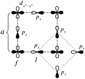
Figure 1: Fig. 1. The $d_{x^{2}-y^{2}}$-orbitals of fermions on copper ions and $p_{x}$ and $p_{y}$ orbitals of fermions at the oxygen ions on the CuO₂ plane, which are taken into account in the Emery model. The dashed lines bound the unit cell with parameter $a$. The dotted lines connect four oxygen orbitals that are closest to the copper orbital.

2 HAMILTONIAN OF THE EMERY MODEL

It is well known that the main features of the electronic structure of the CuO₂ plane in HTSCs is correctly described by the Emery model [11, 12, 14], in which the Hamiltonian in the representation of the secondary quantization operators can be written in the form

$$\hat{H}=\hat{H}_{0}+\hat{U}_{p}+\hat{T}_{pd}+\hat{T}_{pp}+\hat{V}_{pp},$$ (1)

$$\hat{H}_{0}=\varepsilon_{d}\sum_{f}\hat{n}^{d}_{f}+U_{d}\sum_{f}\hat{n}^{d}_{f\uparrow}\hat{n}^{d}_{f\downarrow}+\varepsilon_{p}\sum_{l}\hat{n}^{p}_{l}$$

$$\qquad+V_{pd}\sum_{f\delta}\hat{n}^{d}_{f}\hat{n}^{p}_{f+\delta},$$

$$\hat{U}_{p}=U_{p}\sum_{l}\hat{n}^{p}_{l\uparrow}\hat{n}^{p}_{l\downarrow},\qquad\hat{T}_{pp}=\sum_{l\Delta\sigma}t_{pp}(\Delta)p^{\dagger}_{l\sigma}p_{l+\Delta,\sigma},$$

$$\hat{T}_{pd}=t_{pd}\sum_{f\delta\sigma}\vartheta(\delta)(d^{\dagger}_{f\sigma}p_{f+\delta,\sigma}+\textrm{h.c.}),$$

$$\hat{T}_{pp}=\sum_{l\Delta\sigma}t_{pp}(\Delta)p^{\dagger}_{l\sigma}p_{l+\Delta,\sigma},$$

$$\hat{V}_{pp}=\sum_{ll^{\prime}(l\neq l^{\prime})}V_{pp}(l-l^{\prime})\hat{n}^{p}_{l}\hat{n}^{p}_{l^{\prime}}.$$

Here $d_{f\sigma}^{\dagger}(d_{f\sigma})$ and $p_{l\sigma}^{\dagger}(p_{l\sigma})$ are the creation (annihilation) operators for the $d$- and $p$-fermions, respectively, at copper $f$ and oxygen $l$ sites with spin projections $\sigma=+1/2,-1/2$. One of the four vectors connecting the copper ion with the oxygen ions in the CuO₂ plane is denoted by $\delta=\{\pm x/2,~{}\pm y/2\}$, where $x=(a,0)$ and $y=(0,a)$, $a$ being the unit cell parameter. Vector $\delta$ connects the copper ion at site $f$ with the oxygen ions in the position $l=f+\delta$ (Fig. 1). The particle number operators at copper and oxygen ions are defined as $\hat{n}^{d}_{f}=\sum_{\sigma}\hat{n}^{d}_{f\sigma}=\sum_{\sigma}d_{f\sigma}^{\dagger}d_{f\sigma}$ $\hat{n}^{p}_{l}=\sum_{\sigma}\hat{n}^{p}_{l\sigma}=\sum_{\sigma}p_{l\sigma}^{\dagger}p_{l\sigma}$. By $\varepsilon_{d}$ and $\varepsilon_{p}$ we denote the bare on-site energies of fermions on copper and oxygen ions, respectively. Parameters $U_{d}$ and $U_{p}$ in the Hamiltonian indicate the Coulomb repulsion energy for two particles with opposite spin projections at a copper and an oxygen site, respectively; $V_{pd}$ is the Coulomb repulsion energy for fermions at the copper and oxygen ions, and $V_{pp}$ is the parameter of the Coulomb interaction of fermions at oxygen ions. By $t_{pd}$ we denote the hopping integral for a charge carrier from an oxygen ion to a copper ion. Function $\vartheta(\delta)$ takes into account the effect of the relation between the phases of copper and oxygen orbitals on the hybridization processes. For the orbital profiles shown in Fig. 1, function $\vartheta(\delta)$ assumes the following values upon the variation of $\delta$: $\vartheta(\delta)=\mp 1$ for $\delta=\pm x/2$ or $\delta=\pm y/2$ [15]. By $t_{pp}(\Delta)=t\cdot\rho(\Delta)$, we denote the fermion hopping integral between nearest oxygen orbitals. Its sign is determined by function $\rho(\Delta)$, where vector $\Delta$ connects the nearest oxygen ions. For the chosen sequence of phases of oxygen orbitals, $\rho(\Delta)=1$ for $\Delta=\pm(x+y)/2$ and $\rho(\Delta)=-1$ if $\Delta=\pm(x-y)/2$.

The Hamiltonian of the Emery model is a typical Hamiltonian in the multiband theory of metals in the tight-binding approximation. It belongs to the Hubbard type (the Emery model is often referred to in the literature as the three-band or extended Hubbard model) because it describes both intraatomic Coulomb correlations and hopping between one-ion states of copper and oxygen. However, the Emery model is more realistic as compared to the Hubbard model because it takes into account the chemical composition of copper oxides.

3 SPIN-FERMION MODEL

According to experimental data, in the undoped state with one hole per unit cell, the system is in the state of a Mott-Hubbard insulator [2]. In the Emery model, this corresponds to the SEC regime

$$\Delta_{pd},\,(U_{d}-\Delta_{pd})\gg t_{pd}>0.$$ (2)

These inequalities require, on the one hand, that the Coulomb correlations at the copper ion be taken into account correctly; on the other hand, these inequalities make it possible to carry out the reduction of the Hamiltonian in the Emery model and to obtain the SFM [31, 32, 33, 34, 35, 36]:

$$\hat{H}_{\textrm{sp-f}}=\hat{H}_{\textrm{h}}+\hat{U}_{p}+\hat{V}_{pp}+\hat{J}+\hat{I},$$ (3)

where

$$\hat{H}_{\textrm{h}}=\sum_{k\alpha}\Bigl{(}\xi_{k_{x}}a_{k\alpha}^{\dagger}a_{k\alpha}+\xi_{k_{y}}b_{k\alpha}^{\dagger}b_{k\alpha}$$

$$\qquad+t_{k}(a_{k\alpha}^{\dagger}b_{k\alpha}+b_{k\alpha}^{\dagger}a_{k\alpha})\Bigr{)},$$ (4)

$$\hat{U}_{p}=\frac{U_{p}}{N}\sum_{1,2,3,4}[a^{{\dagger}}_{1\uparrow}a^{{\dagger}}_{2\downarrow}a_{3\downarrow}a_{4\uparrow}+(a\to b)]~{}\delta_{1+2-3-4},$$ (5)

$$\hat{V}_{pp}=\frac{4V_{1}}{N}\sum_{1,2,3,4\atop{\alpha\beta}}\phi_{3-2}~{}a^{{\dagger}}_{1\alpha}b^{{\dagger}}_{2\beta}b_{3\beta}a_{4\alpha}~{}\delta_{1+2-3-4},$$ (6)

$$\hat{J}=\frac{J}{N}\sum_{fkq\alpha\beta}e^{if(q-k)}u_{k\alpha}^{{\dagger}}(\textbf{S}_{f}\boldsymbol{\sigma}_{\alpha\beta})u_{q\beta},$$ (7)

$$\hat{I}=\frac{I}{2}\sum_{f\delta}\textbf{S}_{f}\textbf{S}_{f+2\delta}.$$ (8)

The relation between the operators of the oxygen subsystem in the initial Emery model and the secondary quantization operators in the SFM in the momentum representation is established by the relations

$$p_{f\pm\frac{x}{2},\sigma}=\frac{1}{\sqrt{N}}\sum_{k}e^{ik(f\pm\frac{x}{2})}a_{k\sigma},$$

$$p_{f\pm\frac{y}{2},\sigma}=\frac{1}{\sqrt{N}}\sum_{k}e^{ik(f\pm\frac{y}{2})}b_{k\sigma}.$$ (9)

Operators $a_{k\sigma}$ and $b_{k\sigma}$ correspond to the annihilation of a hole with momentum $k$ and spin projection $\sigma$, respectively, in the $x$- and $y$-sublattices of the oxygen ions.

In the expression for the Hamiltonian $\hat{H}_{\textrm{h}}$, we have introduced the functions

$$\xi_{k_{x(y)}}=\varepsilon_{p}+2V_{pd}+\tau(1-\cos k_{x(y)})-\mu,$$ (10)

where $\mu$ is the chemical potential and parameter $\tau=t^{2}_{pd}/\Delta_{pd}$. The function

$$t_{k}=(2\tau-4t)~{}\psi_{k},$$ (11)

$$\psi_{k}=s_{k,x}s_{k,y},\qquad s_{k,x(y)}=\sin\frac{k_{x(y)}}{2}$$ (12)

describes the hybridization processes in the second order of perturbation theory (parameter $\tau$) as well as direct hopping of holes between the oxygen ions (parameter $t$). The dependence for the sign of the hopping integrals on the direction of vector $\Delta$ leads to the emergence of function $\psi_{k}$ in expression (11).

For brevity, the momenta over which the summation is performed are denoted by $1,\ldots,4$. The delta function $\delta_{1+2-3-4}$ in the above expressions takes into account the momentum conservation law. For operator $\hat{V}_{pp}$ of the intersite Coulomb repulsion, we take into account the interactions only between the nearest oxygen ions. The intensity of these interactions is characterized by parameter $V_{1}$. Function $\phi_{k}$ in $\hat{V}_{pp}$ is defined as

$$\phi_{k}=\cos(k_{x}/2)\cos(k_{y}/2).$$ (13)

Operator $\hat{J}$ describes in the $k$ representation both spincorrelated hopping of holes between oxygen ions and the exchange interaction of a hole at the oxygen ion with the spins at the nearest copper ions. Parameter $J$ of this interaction is defined as $J=4t^{2}_{pd}/\Delta_{pd}$. In operator $\hat{J}$, $\textbf{S}_{f}$ denotes the vector operator of the spin localized at site $f$, while vector operator $\boldsymbol{\sigma}$ is composed of the Pauli matrices: $\boldsymbol{\sigma}=(\sigma^{x},\sigma^{y},\sigma^{z})$. For brevity of notation, we have introduced in expression (7) the operator

$$\quad u_{k\beta}=s_{k,x}a_{k\beta}+s_{k,y}b_{k\beta}.$$ (14)

The last term $\hat{I}$ in the Hamiltonian (3) appears in the fourth order of perturbation theory and describes the exchange interaction of spins localized at copper ions.

The Hamiltonian in the SFM in the momentum representation was considered earlier in [38], where the spectrum of the Fermi quasiparticles in Sr₂CuO₂Cl₂ was analyzed in the self-consistent Born approximation. However, the Coulomb interaction operators $\hat{V}_{pd}$, $\hat{U}_{p}$ and $\hat{V}_{pp}$ were not taken into account.

When deriving expression (3) for the Hamiltonian in the SFM, we assumed that the Coulomb repulsion parameter for holes at copper ions was $U_{d}=\infty$. In further analysis of the conditions for the evolution of the Cooper instability in the SFM, we will use the wellestablished values of parameters for the Emery model [40, 39]: $t_{pd}=1.3,\,\Delta_{pd}=3.6,\,U_{p}=4.0,\,V_{pd}=1.2$ (in eV). For the hole hopping integral at oxygen, we will use the value of $t=0.12$ eV [45], and the exchange interaction constant between the spins of the copper ions is chosen to be $I=0.136$ eV, which is in conformity with the available experimental data on cuprate superconductors. The parameter of the intersite Coulomb repulsion of holes is chosen as $V_{1}=1\div 2$ eV [37].

4 EQUATIONS FOR THE GREEN FUNCTIONS

An important feature of the SFM is that the exchange coupling between localized spins and the spins of holes turns out to be strong: $J=1.88$ eV $\gg\tau\approx 0.47$ eV. This means that when describing the oxygen ion subsystem, the strong coupling between holes at oxygen ions and the subsystems of spins at copper ions must be taken into account exactly. For this purpose, it is convenient to use the Zwanzig-Mori projection method [41, 42, 43]. The method for calculating the dispersion curves for spin-polaron excitations in the SFM, which is based on this approach, was described in detail in [44] and was actively used in subsequent studies [45, 46, 47].

For taking into account the aforementioned strong spin-charge coupling, it is necessary to introduce one more operator into the basis set of operators (apart of operators $a_{k\alpha}$ and $b_{k\alpha}$), viz.,

$$L_{k\alpha}=\frac{1}{N}\sum_{fq\beta}e^{if(q-k)}(\textbf{S}_{f}\boldsymbol{\sigma}_{\alpha\beta})u_{q\beta}.$$ (15)

For analyzing the conditions for Cooper instability, we must supplement the above set of three operators with three extra operators [30, 47] ($\bar{\alpha}~{}=~{}-\alpha$)

$$a_{-k\bar{\alpha}}^{{\dagger}},\quad b_{-k\bar{\alpha}}^{{\dagger}},\quad L_{-k\bar{\alpha}}^{{\dagger}}.$$ (16)

The addition of these operators to the basis makes it possible to analyze not only normal, but also anomalous thermodynamic means using a unified approach.

The exact equations of motion for the first three basis operators have the form

$$i\frac{da_{k\uparrow}}{dt}=\xi_{k_{x}}a_{k\uparrow}+t_{k}b_{k\uparrow}+Js_{k,x}L_{k\uparrow}$$

$$\qquad+\frac{U_{p}}{N}\sum_{1,2,3}a^{{\dagger}}_{1\downarrow}a_{2\downarrow}a_{3\uparrow}\delta_{k+1-2-3}$$

$$\qquad+\frac{4V_{1}}{N}\sum_{1,2,\alpha}\phi_{k-2}~{}b^{{\dagger}}_{1\alpha}b_{1-2+k,\alpha}a_{2\uparrow},$$ (17)

$$i\frac{db_{k\uparrow}}{dt}=\xi_{k_{y}}b_{k\uparrow}+t_{k}a_{k\uparrow}+Js_{k,y}L_{k\uparrow}$$

$$\qquad+\frac{U_{p}}{N}\sum_{1,2,3}b^{{\dagger}}_{1\downarrow}b_{2\downarrow}b_{3\uparrow}\delta_{k+1-2-3}$$

$$+\frac{4V_{1}}{N}\sum_{1,2,\alpha}~{}\phi_{1-2}~{}a^{{\dagger}}_{1\alpha}a_{2\alpha}b_{1-2+k,\uparrow},$$ (18)

$$i\frac{dL_{k\uparrow}}{dt}=\sum_{q\beta}(\textbf{S}_{k-q}\boldsymbol{\sigma}_{\uparrow\beta})\left[\Bigl{(}\xi_{q_{x}}s_{q,x}+t_{q}s_{q,y}\Bigr{)}a_{q\beta}\right.$$

$$\left.+\Bigl{(}\xi_{q_{y}}s_{q,y}+t_{q}s_{q,x}\Bigr{)}b_{q\beta}\right]$$

$$+\frac{U_{p}}{N}\sum_{1,2,3,4}\delta_{1-2+3-4}\left[s_{1,x}(\textbf{S}_{k-1}\boldsymbol{\sigma}_{\downarrow\alpha})a^{{\dagger}}_{3\alpha}a_{4,\downarrow}a_{2\uparrow}\right.$$

$$\left.+s_{1,y}(\textbf{S}_{k-1}\boldsymbol{\sigma}_{\downarrow\alpha})b^{{\dagger}}_{3\alpha}b_{4,\downarrow}b_{2\uparrow}\right]$$

$$+\frac{4V_{1}}{N}\sum_{1,2,3\atop{\alpha\beta}}\phi_{1-2}\left[s_{1,x}(\textbf{S}_{k-1}\boldsymbol{\sigma}_{\uparrow\alpha})b^{{\dagger}}_{3\beta}b_{1-2+3,\beta}a_{2\alpha}\right.$$

$$\left.+s_{3,y}(\textbf{S}_{k-3}\boldsymbol{\sigma}_{\uparrow\alpha})a^{{\dagger}}_{1\beta}a_{2\beta}b_{1-2+3,\alpha}\right]$$

$$+J\sum_{qp\alpha\beta}s^{2}_{p}(\textbf{S}_{k-p}\boldsymbol{\sigma}_{\uparrow\alpha})(\textbf{S}_{p-q}\boldsymbol{\sigma}_{\alpha\beta})u_{q\beta}$$

$$+\frac{iJ}{N}\sum_{pqq_{1}\atop{\alpha\beta\nu}}(\boldsymbol{\sigma}_{\uparrow\nu}\times\boldsymbol{\sigma}_{\alpha\beta})\textbf{S}_{k+p-q-q_{1}}u^{{\dagger}}_{p\alpha}u_{q\beta}u_{q_{1}\nu}$$

$$-4iI\sum_{qp\alpha}\gamma_{1p}u_{q\alpha}\boldsymbol{\sigma}_{\uparrow\alpha}(\textbf{S}_{k-q+p}\times\textbf{S}_{-p}),$$ (19)

where $s^{2}_{k}=s^{2}_{k,x}+s^{2}_{k,y}$, and invariant $\gamma_{1p}$ of the square lattice will be defined later (see relation (4) below). In addition, in equation of motion (4), we have introduced the Fourier transform of the spin operator

$$\textbf{S}_{k}=\frac{1}{N}\sum_{f}e^{-ikf}\textbf{S}_{f}.$$

Within the projection method [41, 42], the system of the equations of motion for the Green functions can be written as

$$\omega~{}{\hat{G}}(k,\omega)=\hat{K}(k)+\hat{D}(k)\hat{K}^{-1}(k)~{}{\hat{G}}(k,\omega),$$ (20)

where the matrix retarded Green function is defined by elements ${G}_{ij}(k,\omega)=\langle\langle A_{ik}|A^{{\dagger}}_{jk}\rangle\rangle_{\omega}$, and the elements of the energy matrix $\hat{D}(k)$ and the normalization matrix $\hat{K}(k)$ are defined as

$$D_{ij}(k)=\langle\{[A_{ik},\hat{H}_{\textrm{sp-f}}],A^{{\dagger}}_{jk}\}\rangle,$$

$$K_{ij}(k)=\langle\{A_{ik},A^{{\dagger}}_{jk}\}\rangle.~{}~{}~{}$$ (21)

Operators $A_{ik}$ on the right-hand sides of these expressions run through a set of six basis operators

$$\{a_{k\uparrow},b_{k\uparrow},L_{k\uparrow},a^{{\dagger}}_{-k\downarrow},b^{{\dagger}}_{-k\downarrow},L^{{\dagger}}_{-k\downarrow}\},$$

and the angle brackets in relation (4) denote thermodynamic mean.

Evaluating elements (4) and substituting them into matrix equation (20), we obtain a closed system of equations for the normal $G_{ij}$ and anomalous $F_{ij}$ Green functions ($j=1,2,3$)

$$(\omega-\xi_{x})G_{1j}=\delta_{1j}+t_{k}G_{2j}+J_{x}G_{3j}+\Delta_{1k}F_{1j}+\Delta_{2k}F_{2j},$$

$$(\omega-\xi_{y})G_{2j}=\delta_{2j}+t_{k}G_{1j}+J_{y}G_{3j}+\Delta_{3k}F_{1j}+\Delta_{4k}F_{1j},$$

$$(\omega-\xi_{L})G_{3j}=\delta_{3j}K_{k}+(J_{x}G_{1j}+J_{y}G_{2j})K_{k}+\frac{\Delta_{5k}}{K_{k}}F_{3j},$$

$$(\omega+\xi_{x})F_{1j}=\Delta_{1k}^{*}G_{1j}+\Delta_{3k}^{*}G_{2j}-t_{k}F_{2j}+J_{x}F_{3j},$$

$$(\omega+\xi_{y})F_{2j}=\Delta_{2k}^{*}G_{1j}+\Delta_{4k}^{*}G_{2j}-t_{k}F_{1j}+J_{y}F_{3j},$$

$$(\omega+\xi_{L})F_{3j}=\frac{\Delta^{*}_{5k}}{K_{k}}G_{3j}+(J_{x}F_{1j}+J_{y}F_{2j})K_{k}.$$ (22)

Here, we have introduced the following notation for the normal Green functions:

$$G_{11}=\langle\langle a_{k\uparrow}|a_{k\uparrow}^{{\dagger}}\rangle\rangle_{\omega},\qquad G_{21}=\langle\langle b_{k\uparrow}|a_{k\uparrow}^{{\dagger}}\rangle\rangle_{\omega},$$

$$\qquad\qquad G_{31}=\langle\langle L_{k\uparrow}|a_{k\uparrow}^{{\dagger}}\rangle\rangle_{\omega}.$$

Functions $G_{i2}$ and $G_{i3}$ ($i=1,2,3$) are defined analogously, the only difference being that instead of $a^{{\dagger}}_{k\uparrow}$, we have operators $b^{{\dagger}}_{k\uparrow}$ and $L^{{\dagger}}_{k\uparrow}$, respectively. The anomalous Green functions are defined as

$$F_{11}=\langle\langle a_{-k\downarrow}^{{\dagger}}|a_{k\uparrow}^{{\dagger}}\rangle\rangle_{\omega},\qquad F_{21}=\langle\langle b_{-k\downarrow}^{{\dagger}}|a_{k\uparrow}^{{\dagger}}\rangle\rangle_{\omega},$$

$$\qquad\qquad F_{31}=\langle\langle L_{-k\downarrow}^{{\dagger}}|a_{k\uparrow}^{{\dagger}}\rangle\rangle_{\omega}.$$

For $F_{i2}$ and $F_{i3}$ ($i=1,2,3$), we are using the same notation for the second subscript.

When writing system of equations (4), we have used the following functions:

$$\xi_{x(y)}=\xi_{k_{x(y)}},\quad J_{x(y)}=Js_{k,x(y)},$$

$$\xi_{L}(k)=\tilde{\varepsilon}_{p}-\mu-2t+5\tau/2-J$$

$$\quad\quad+[(\tau-2t)(-C_{1}\gamma_{1k}+C_{2}\gamma_{2k})$$

$$\quad\quad+\tau(-C_{1}\gamma_{1k}+C_{3}\gamma_{3k})/2$$

$$\quad\quad+JC_{1}(1+4\gamma_{1k})/4-IC_{1}(\gamma_{1k}+4)]K_{k}^{-1},$$ (23)

where $K_{k}=\langle\{L_{k\uparrow},L^{{\dagger}}_{k\uparrow}\}\rangle=3/4-C_{1}\gamma_{1k}$, and $\gamma_{jk}$ denote invariants of the square lattice:

$$\gamma_{1k}=(\cos k_{x}+\cos k_{y})/2,$$

$$\gamma_{2k}=\cos k_{x}\,\cos k_{y},$$

$$\gamma_{3k}=(\cos 2k_{x}+\cos 2k_{y})/2.$$ (24)

For the components of the superconductor order parameter, which are defined as

$$\Delta_{1k}=\langle\{[a_{k\uparrow},\hat{H}_{\textrm{sp-f}}],a_{-k\downarrow}\}\rangle,$$

$$\Delta_{2k}=\langle\{[a_{k\uparrow},\hat{H}_{\textrm{sp-f}}],b_{-k\downarrow}\}\rangle,$$

$$\Delta_{3k}=\langle\{[b_{k\uparrow},\hat{H}_{\textrm{sp-f}}],a_{-k\downarrow}\}\rangle,$$

$$\Delta_{4k}=\langle\{[b_{k\uparrow},\hat{H}_{\textrm{sp-f}}],b_{-k\downarrow}\}\rangle,$$

$$\Delta_{5k}=\langle\{[L_{k\uparrow},\hat{H}_{\textrm{sp-f}}],L_{-k\downarrow}\}\rangle,$$ (25)

we obtain

$$\Delta_{1k}=-\frac{U_{p}}{N}\sum_{q}\langle a_{q\uparrow}a_{-q\downarrow}\rangle,$$

$$\Delta_{2k}=-\frac{4V_{1}}{N}\sum_{q}\phi_{k-q}\langle a_{q\uparrow}b_{-q\downarrow}\rangle,$$

$$\Delta_{3k}=-\frac{4V_{1}}{N}\sum_{q}\phi_{k-q}\langle b_{q\uparrow}a_{-q\downarrow}\rangle,$$

$$\Delta_{4k}=-\frac{U_{p}}{N}\sum_{q}\langle b_{q\uparrow}b_{-q\downarrow}\rangle,$$

$$\Delta_{5k}=\frac{1}{N}\sum_{q}\biggl{\{}I_{k-q}\bigl{(}\langle L_{q\uparrow}L_{-q\downarrow}\rangle-C_{1}\langle u_{q\uparrow}u_{-q\downarrow}\rangle\bigr{)}$$

$$\quad+8IC_{1}\langle u_{q\uparrow}u_{-q\downarrow}\rangle\biggr{\}}+\frac{J}{N}\sum_{q}\biggl{\{}-2\gamma_{1q}\langle L_{q\uparrow}L_{-q\downarrow}\rangle$$

$$\quad+\bigl{(}3/2-4C_{1}\gamma_{1k}\bigr{)}\langle u_{q\uparrow}u_{-q\downarrow}\rangle\biggr{\}}$$

$$\quad-\frac{U_{p}}{N}\sum_{q}\biggl{\{}(3/8-C_{1}/2\cos k_{x})\langle a_{q\uparrow}a_{-q\downarrow}\rangle$$

$$\quad+(3/8-C_{1}/2\cos k_{y})\langle b_{q\uparrow}b_{-q\downarrow}\rangle\biggr{\}}$$

$$\quad-\frac{V_{1}}{N}\sum_{q}\biggl{\{}(3/4-2C_{1}\gamma_{1k}+C_{2}\gamma_{2k})\psi_{q}$$

$$\quad+C_{2}\sin k_{x}\sin k_{y}\phi_{q}\biggr{\}}\bigl{(}\langle a_{q\uparrow}b_{-q\downarrow}\rangle+\langle b_{q\uparrow}a_{-q\downarrow}\rangle\bigr{)}$$

$$\quad+\frac{2}{N}\sum_{q}\left(\xi(q_{x})s_{q,x}+t_{q}s_{q,y}\right)\langle a_{q\uparrow}L_{-q\downarrow}\rangle$$

$$\quad+\frac{2}{N}\sum_{q}\left(\xi(q_{y})s_{q,y}+t_{q}s_{q,x}\right)\langle b_{q\uparrow}L_{-q\downarrow}\rangle,$$ (26)

where $I_{k}=4I\gamma_{1k}$, and the mean is given by

$$\langle u_{q\uparrow}u_{-q\downarrow}\rangle = -s^{2}_{q,x}\langle a_{q\uparrow}a_{-q\downarrow}\rangle-s^{2}_{q,y}\langle b_{q\uparrow}b_{-q\downarrow}\rangle$$ (27)

$$-\psi_{q}\bigl{(}\langle a_{q\uparrow}b_{-q\downarrow}\rangle+\langle b_{q\uparrow}a_{-q\downarrow}\rangle\bigr{)}.$$

When deriving expressions (4) and (4), we took into account the fact that the subsystem of spins localized at copper ions is in the state of a quantum spin liquid. In this case, spin correlation functions $C_{j}=\langle S_{0}S_{r_{j}}\rangle$ appearing in expressions (4) and (4), satisfy the relations

$$C_{j}=3\langle S^{x}_{0}S^{x}_{r_{j}}\rangle=3\langle S^{y}_{0}S^{y}_{r_{j}}\rangle=3\langle S^{z}_{0}S^{z}_{r_{j}}\rangle,$$ (28)

where $r_{j}$ is the coordinate of the copper ion in the $j$th. coordination sphere. In this case, $\langle S^{x}_{f}\rangle=\langle S^{y}_{f}\rangle=\langle S^{z}_{f}\rangle=0$.

When deriving the fifth equation in (4) for the mean values of the product of operators that cannot be reduced to the basis operators, we have used the relation

$$\langle\left(\textbf{S}_{f}\boldsymbol{\sigma}_{\downarrow\alpha}c_{k\alpha}\right)\left(\textbf{S}_{g}\boldsymbol{\sigma}_{\uparrow\beta}c_{p\beta}\right)\rangle~{}~{}~{}~{}~{}~{}~{}~{}~{}~{}~{}~{}~{}~{}$$

$$=2\langle\left(\textbf{S}_{f}\textbf{S}_{g}\right)c_{k\uparrow}c_{p\downarrow}\rangle-\langle\left(\textbf{S}_{f}\boldsymbol{\sigma}_{\downarrow\alpha}c_{p\alpha}\right)\left(\textbf{S}_{g}\boldsymbol{\sigma}_{\uparrow\beta}c_{k\beta}\right)\rangle,$$ (29)

where summation over indices $\alpha$ and $\beta$ is implied. Relation (4) is valid in the SU(2) invariant phase and makes it possible to express this mean in terms of the mean value of the basis operators. The anomalous mean $\langle L_{q\uparrow}L_{-q,\downarrow}\rangle$ playing the decisive role in the realization of the $d$-wave superconductivity in the ensemble of spin-polaron quasiparticles appears in the sum in the equation for the order parameter component $\Delta_{5k}$ in the system (4) only when relation (4) is used.For thermodynamic means containing the scalar product of the spin operators, the uncoupling procedure was used. This explains, in particular, the emergence of magnetic correlator $C_{1}$, which is proportional to exchange integral $I$, in the first term on the right-hand side of the expression for $\Delta_{5k}$.

The contributions to $\Delta_{5k}$ from the intersite Coulomb interaction immediately after the evaluation of the commutators have the form

$$-\frac{4V_{1}}{N}\sum_{1,2,3,4\atop{\alpha\beta}}\phi_{1-2}s_{1x}s_{3y}\delta_{1-2+3-4}$$

$$\times\left[\langle(\textbf{S}_{k-1}\boldsymbol{\sigma}_{\uparrow\alpha}a_{2\alpha})(\textbf{S}_{-k-3}\boldsymbol{\sigma}_{\downarrow\beta}b_{4\beta})\rangle\right.$$

$$\left.+\langle(\textbf{S}_{k-3}\boldsymbol{\sigma}_{\uparrow\alpha}b_{4\alpha})(\textbf{S}_{-k-1}\boldsymbol{\sigma}_{\downarrow\beta}a_{2\beta})\rangle\right].$$ (30)

Since the operators in the mean cannot be reduced to basis operators even when relation (4) is used, the uncoupling procedure is employed for the mean values in expression (4) taking into account the SU(2) invariance of the spin subsystem. This procedure leads to the emergence of the term proportional to $V_{1}$ in the fifth equation in (4).

It should also be noted that since we are interested in the weak doping regime, the contributions appearing in expressions (4) and (4) as a result of uncoupling of the means and proportional to correlators of the density-density type are not considered here.

Analysis of system of equations (4) in the normal phase leads to the conclusion that the Fermi excitation spectrum in the SFM is determined by the solutions to the dispersion equation

$$\mathrm{det}_{k}(\omega)=(\omega-\xi_{x})(\omega-\xi_{y})(\omega-\xi_{L})-2J_{x}J_{y}t_{k}K_{k}$$

$$-(\omega-\xi_{y})J_{x}^{2}K_{k}-(\omega-\xi_{x})J_{y}^{2}K_{k}-(\omega-\xi_{L})t_{k}^{2}=0,~{}$$ (31)

and contains three branches: $\epsilon_{1k}$, $\epsilon_{2k}$ and $\epsilon_{3k}$ [47]. Lower branch $\epsilon_{1k}$ is characterized by a minimum near point ($\pi/2$, $\pi/2$) of the Brillouin zone and is separated considerably from the two upper branches $\epsilon_{2k}$ and $\epsilon_{3k}$. The lower branch appears due to the strong spin charge coupling that induces the exchange interaction between holes and localized spins at the nearest copper ions, as well as spin-correlated hopping. At low doping levels, the dynamics of holes at oxygen ions is determined predominantly by the lower branch $\epsilon_{1k}$.

5 SYSTEM OF EQUATIONS FOR THE SUPERCONDUCTING ORDER PARAMETER COMPONENTS

For analyzing the conditions for the Cooper instability, let us express the required anomalous Green functions in terms of parameters $\Delta^{*}_{lk}$. in the linear approximation. These functions have the form

$$F_{ij}(k,\omega)=\sum_{i,j=1}^{3}\sum_{l=1}^{5}\frac{S_{ij}^{(l)}(k,\omega)}{{\rm Det}_{k}(\omega)}\Delta_{lk}^{*}.$$ (32)

The Green functions required for analyzing the conditions for the emergence of superconductivity are $F_{11}(k,\omega)$, $F_{12}(k,\omega)$, $F_{21}(k,\omega)$, $F_{22}(k,\omega)$, $F_{31}(k,\omega)$, $F_{32}(k,\omega)$ and $F_{33}(k,\omega)$. Here, $\textrm{Det}_{k}(\omega)=-\textrm{det}_{k}(\omega)\textrm{det}_{k}(-\omega)$, and corresponding functions $S_{ij}^{(l)}(k,\omega)$ are given in Appendix A.

Using the spectral theorem [48], we obtain the following expressions for anomalous means and the closed system of homogeneous integral equations for the superconducting order parameter components ($l=1,\ldots,5$)

$$\Delta_{1k}^{*}=-\frac{U_{p}}{N}\sum_{lq}M^{(l)}_{11}(q)\Delta_{lq}^{*},$$ (33)

$$\Delta_{2k}^{*}=-\frac{4V_{1}}{N}\sum_{lq}\phi_{k-q}M^{(l)}_{21}(q)\Delta_{lq}^{*},$$

$$\Delta_{3k}^{*}=-\frac{4V_{1}}{N}\sum_{lq}\phi_{k-q}M^{(l)}_{12}(q)\Delta_{lq}^{*},$$

$$\Delta_{4k}^{*}=-\frac{U_{p}}{N}\sum_{lq}M^{(l)}_{22}(q)\Delta_{lq}^{*},$$

$$\Delta_{5k}^{*}=-\frac{1}{N}\sum_{lq}R^{(l)}_{0}(q)\Delta_{lq}^{*}+\frac{1}{N}\sum_{lq}I_{k-q}R^{(l)}_{1a}(q)\Delta_{lq}^{*}$$

$$\quad+\cos k_{x}\frac{1}{N}\sum_{lq}R^{(l)}_{1b}(q)\Delta_{lq}^{*}+\cos k_{y}\frac{1}{N}\sum_{lq}R^{(l)}_{1c}(q)\Delta_{lq}^{*}$$

$$\quad-\gamma_{2k}\frac{1}{N}\sum_{lq}\psi_{q}R^{(l)}_{2}(q)\Delta_{lq}^{*}$$

$$\quad-\sin k_{x}\sin k_{y}\frac{1}{N}\sum_{lq}\phi_{q}R^{(l)}_{2}(q)\Delta_{lq}^{*},$$

where the following functions have been introduced:

$$R^{(l)}_{0}(q)=\displaystyle\frac{3}{4}V_{1}\psi_{q}M^{(l)}_{ab}(q)+2J\gamma_{1q}M^{(l)}_{33}(q)$$

$$\quad-(8IC_{1}+3J/2)M^{(l)}_{uu}(q)+\displaystyle\frac{3}{8}U_{p}(M^{(l)}_{11}(q)+M^{(l)}_{22}(q))$$

$$\quad-2\left(\xi(q_{x})s_{q,x}+t_{q}s_{q,y}\right)M^{(l)}_{31}(q)$$

$$\quad-2\left(\xi(q_{y})s_{q,y}+t_{q}s_{q,x}\right)M^{(l)}_{32}(q),$$

$$R^{(l)}_{1a}(q)=M^{(l)}_{33}(q)-C_{1}M^{(l)}_{uu}(q),$$

$$R^{(l)}_{1b}(q)=C_{1}(V_{1}\psi_{q}M^{(l)}_{ab}(q)-2JM^{(l)}_{uu}(q)+U_{p}M^{(l)}_{11}(q)),$$

$$R^{(l)}_{1c}(q)=C_{1}(V_{1}\psi_{q}M^{(l)}_{ab}(q)-2JM^{(l)}_{uu}(q)+U_{p}M^{(l)}_{22}(q)),$$

$$R^{(l)}_{2}(q)=V_{1}C_{2}M^{(l)}_{ab}(q),$$ (34)

$$M^{(l)}_{uu}(q)=-s_{qx}^{2}M^{(l)}_{11}(q)-s_{qy}^{2}M^{(l)}_{22}(q)-\psi_{q}M^{(l)}_{ab}(q),$$

$$M^{(l)}_{ab}(q)=M^{(l)}_{21}(q)+M^{(l)}_{12}(q),$$

$$M^{(l)}_{nm}(q)=\frac{S^{(l)}_{nm}(q,E_{1q})+S^{(l)}_{nm}(q,-E_{1q})}{4E_{1q}(E_{1q}^{2}-E_{2q}^{2})(E_{1q}^{2}-E_{3q}^{2})}\tanh\left(\frac{E_{1q}}{2T}\right).$$

System of equations (33) will be used below for determining the temperature of transition of an ensemble of polarons to the superconducting state with preset type of order parameter symmetry.

6 COMPETITION OF $d$- AND $s$-WAVE PAIRINGS OF SPIN POLARONS TAKING INTO ACCOUNT THE COULOMB INTERACTIONS

It can be seen from system (33) that the kernels of integral equations are uncoupled; therefore, the solution to this system can be sought in the form

$$\Delta_{1k}=B_{1},$$

$$\Delta_{2k}=B_{1\phi}\phi_{k}+B_{1\psi}\psi_{k},$$

$$\Delta_{3k}=B_{2\phi}\phi_{k}+B_{2\psi}\psi_{k},$$

$$\Delta_{4k}=B_{2},$$

$$\Delta_{5k}=B_{3}+B_{cx}\cos k_{x}+B_{cy}\cos k_{y}$$

$$\qquad+B\cos{k_{x}}\cos{k_{y}}+B_{ss}\sin{k_{x}}\sin{k_{y}},$$ (35)

where eleven amplitudes $B_{j}$ ($j=1,1\phi,1\psi,...$) determine the contribution of the corresponding basis functions to the expansion of the order parameter components. Substituting these expressions into Eqs. (33) and equating the coefficients of the corresponding trigonometric functions, we obtain the system of eleven algebraic equations for determining amplitudes $B_{j}$. Actually, the situation is simplified because the system splits into two independent subsystems. The first subsystem defines three amplitudes ($B_{1\phi}$, $B_{2\phi}$ and $B_{ss}$). Numerical calculations show that in the entire doping range of interest, this system has no solutions and will not be considered here.

The second subsystem of equations defines the remaining eight amplitudes $B_{j}$, which can be conveniently written in the form of a column vector

$$B=(B_{3},B_{cx},B_{cy},B_{cc},B_{1\psi},B_{2\psi},B_{1},B_{2})^{T}.$$ (36)

In matrix form, the system of eight equations can be written as

$$B=\hat{W}B,$$ (37)

where components of eighth-order matrix $\hat{W}$ can be calculated using the expressions

$$W_{ij}=\frac{1}{N}\sum_{k}w_{ij}(k),~{}~{}~{}(i,j=1,\dots,8),$$ (38)

and functions $w_{ij}(q)$ are given in Appendix B.

To determine the dependence of superconducting transition temperature $T_{c}$ on doping level $x$ for different types of the order parameter symmetry, we should solve Eq. (37) together with the equation for chemical potential $\mu$. In deriving the equation for $\mu$, we should take into account the fact that all order parameters $\Delta_{jk}\to 0$ in the limit of interest $T\to T_{c}$. As a result, we obtain the following equation for determining the chemical potential:

$$x=\frac{2}{N}\sum_{q}\frac{f(\epsilon_{1q})\left[Q_{3x}(q,\epsilon_{1q})+Q_{3y}(q,\epsilon_{1q})\right]}{\left(\epsilon_{1q}-\epsilon_{2q}\right)\left(\epsilon_{1q}-\epsilon_{3q}\right)},$$ (39)

where $f(E)=(e^{E/T}+1)^{-1}$ is the Fermi-Dirac distribution function.

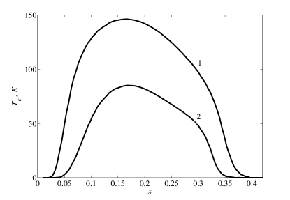
Figure 2: Fig. 2. Doping dependences of the superconducting transition temperature for the $d_{x^{2}-y^{2}}$-wave pairing, obtained for the model parameters $J$=1.88, $\tau$ =0.47, $t$=0.12, $I$=0.136. Curves 1 and 2 describe $T_{c}(x)$ for $U_{p}=0$ and $U_{p}=3$, respectively. The inclusion of intersite Coulomb interaction $V_{1}$ does not influence on these dependencies. All energy parameters are given in eV.

The results of numerical self-consistent solution of system of equations (37) together with equation (39), for the chemical potential are represented in Fig. 2. Solid curve 1 shows the dependence of the critical temperature of superconducting $d_{x^{2}-y^{2}}$-wave pairing on the doping level for $U_{p}=0$ and $V_{1}=0$. This curve was obtained earlier in [47] and is in good agreement with experimental data on the absolute value of $T_{c}$ and on the doping region in which the Cooper instability evolves.

An important aspect of the approach developed here is that the inclusion of Coulomb interaction $V_{1}$ of fermions located at the nearest oxygen ions does not affect the $T_{c}(x)$ dependence for the superconducting $d_{x^{2}-y^{2}}$-wave pairing: curve 1 in Fig. 2 remains unchanged [30]. The cause for such a behavior can be found after analysis of the solutions to system of integral equations (33). In the doping interval in which the above type of pairing is realized for $T\lesssim T_{c}$, the solutions to algebraic system (37) for the amplitudes are such that only four amplitudes $B_{cx}$, $B_{cy}$, $B_{1\psi}$ and $B_{2\psi}$ differ from zero and $B_{cx}=-B_{cy}$, $B_{1\psi}=-B_{2\psi}$, and $|B_{cx}|/|B_{1\psi}|\sim 10^{3}$. This means that the dependence of the superconducting gap on $k$ is mainly due to the fifth component $\Delta_{5k}$ of superconducting order parameter, which in this case has the form

$$\Delta^{(d)}_{5k}=B_{cx}\cdot(\cos k_{x}-\cos k_{y}).$$ (40)

Since for the $d$-wave pairing for $U_{p}=0$, amplitudes $B_{cx}$ and $B_{cy}$ in the equation for $\Delta_{5k}$ are determined not by parameter $V_{1}$, but by the exchange coupling constant $I$ alone, we arrive at the conclusion that the Coulomb repulsion of holes located at neighboring oxygen sites do not suppress the superconducting phase with the $d_{x^{2}-y^{2}}$-wave order parameter symmetry [30].

This means that in the case of the $d$-wave pairing and $U_{p}=0$, we can obtain instead of system (37) a simpler equation for the superconducting transition temperature $T_{c}$ [47, 49, 50]. This equation follows from the fifth equation of system (33) and has the form

$$1=\frac{I}{N}\sum_{q}(\cos q_{x}-\cos q_{y})^{2}$$

$$\qquad\times\left(M_{33}^{(5)}(q,\epsilon_{1q})-C_{1}M_{uu}^{(5)}(q,\epsilon_{1q})\right).$$ (41)

This equation implies, in particular, that the exchange interaction of spin moments of the copper ions, which is transformed into effective attraction as a result of the strong spin-charge coupling, is the mechanism of the Cooper instability. The results of solution of Eq. (6) and system (37) for the $d$-wave pairing and $U_{p}=0$ obviously coincide and correspond to solid curve 1 in Fig. 2.

In contrast to the intersite interaction, the allowance for the Coulomb interaction $U_{p}$ of two holes at oxygen ion leads to the suppression of the superconducting $d$-wave phase. However, as it follows from comparison of the curve 2 ($U_{p}=3$ eV) and the curve 1 ($U_{p}=0$) in Fig. 2, this suppression is not essential for the implementation of HTSC, since in the region of optimal doping $x\simeq 0.16$ the critical temperature remains high.

From the system of integral equations (33) it follows that the solution corresponding to the $s$-phase should have the form

$$\Delta^{(s)}_{1k}=\Delta^{(s)}_{4k}=B_{1},$$

$$\Delta^{(s)}_{2k}=\Delta^{(s)}_{3k}=0,$$

$$\Delta^{(s)}_{5k}=B_{3}+2B_{cx}\gamma_{1k}+B_{cc}\gamma_{2k}.$$ (42)

Calculations show that for all realistic parameters of the model there is no non-trivial solution. Consequently, in the SFM, when the strong coupling of holes on oxygen ions with spin moments of copper ions is correctly taken into account, the superconducting phase with the $s$-wave symmetry of the order parameter is not realized. This is the main difference between the theory of HTSC developed here and the approaches based on the effective single-band models of strongly correlated fermions on the square lattice, in which along with the superconducting $d$-wave pairing there is always a solution for the superconducting $s$-wave pairing.

7 CONCLUSION

The main results of this study can be formulated as follows.

(1) It has been shown that the neutralization for the negative effect of the intersite Coulomb interaction of holes in the oxygen subsystem on the Cooper instability in the $d$-wave channel occurs as a result of two factors. The first factor is associated with the analysis of the actual crystallographic structure of the CuO₂ plane, according to which the Coulomb repulsion of fermions in the oxygen sublattice is determined by the Fourier transform of intersite interaction $V_{q}=4V_{1}\cos(q_{x}/2)\cos(q_{y}/2)$. The second factor is associated with the electron correlations leading to the emergence of strong coupling between the localized spins of copper ions and holes at the oxygen ions. As a result, the spin-polaron quasiparticles are formed and move over the copper ion sublattice; in the ensemble of these particles, the Cooper instability evolves. The Coulomb repulsion between bare holes with the Fourier transform $V_{q}$ is renormalized into the interaction between spin-polaron quasiparticles so that the momentum dependence of this effective interaction corresponds to the structure of the copper ion sublattice. As a result, the situation takes place, when the effective repulsion between the spin polarons falls out of the equation for the superconducting order parameter with the $d$-wave symmetry. At the same time, the contribution of such an effective repulsion remains for the Cooper instability in the $s$-wave channel.

(2) The solution of the system of self-consistent integral equations for superconducting phases showed that in the spin-fermion model only the phase with the $d$-wave symmetry of the order parameter is realized, whereas solutions for the $s$-wave pairing are not available for all the admissible levels of doping. These results completely correspond to the experimental data on cuprate superconductors. In this connection, we note that within the $t-J$ model, the superconducting $s$-wave pairing is realized, and the critical temperature corresponding to this phase is much higher than $T_{c}$ for the $d$-wave pairing. Concerning the differences that arise, it is appropriate to point out that in our approach the spin subsystem of copper ions, separated from the hole subsystem, plays an important role, whereas within the $t-J$ model the electron and spin degrees of freedom are due to the same electrons.

(3) The effect of Coulomb repulsion $U_{p}$ for quasiparticles at the same oxygen ion on the dependence of the superconducting transition temperature for superconducting phase with the $d$-wave symmetry of the order parameter on the doping level has been analyzed. It is shown that taking $U_{p}$ into account leads to decrease in the superconducting transition temperature, but this temperature remains within the limits that are observed experimentally.

It should also be noted that the different contributions of the Coulomb interaction to the conditions of realization of the superconducting phases with different symmetries of the order parameter are manifested, for example, in the Kohn-Luttinger theory of superconductivity [51]. In our case, the separation factor plays a decisive role, when two types of oxygen orbitals spatially separated from the spins of the copper ions are taken into account.

8 ACKNOWLEDGMENTS

This work was supported by the Russian Foundation for Basic Research (RFBR), the Government of Krasnoyarsk Region, the Krasnoyarsk Region Science and Technology Support Fund (projects nos. 16-42-240435, 16-42-243056 and 16-42-243057), and the Program by SB RAS (project no. 356-2015-0406). The work of A. F. B. was supported by the RFBR (project no. 16-02-00304). The work of M. M. K. was supported by the Council for Grants of the President of the Russian Federation (MK-1398.2017.2).

Appendix A

Functions $S_{ij}^{(l)}(k,\omega)$ appearing in the expressions for anomalous Green functions $F_{ij}(k,\omega)$ (32) have the form

$$S^{(1)}_{11}(k,\omega)=Q_{3y}(k,-\omega)Q_{3y}(k,\omega),$$

$$S^{(2)}_{11}(k,\omega)=S^{(1)}_{21}(k,\omega)=Q_{3}(k,-\omega)Q_{3y}(k,\omega),$$

$$S^{(3)}_{11}(k,\omega)=S^{(1)}_{12}(k,\omega)=S^{(2)}_{11}(k,-\omega),$$

$$S^{(4)}_{11}(k,\omega)=S^{(2)}_{12}(k,\omega)=S^{(3)}_{21}(k,\omega)=S^{(1)}_{22}(k,\omega)$$

$$\qquad\qquad=Q_{3}(k,-\omega)Q_{3}(k,\omega),$$

$$S^{(5)}_{11}(k,\omega)=-Q_{y}(k,-\omega)Q_{y}(k,\omega),$$

$$S^{(3)}_{12}(k,\omega)=Q_{3y}(k,-\omega)Q_{3x}(k,\omega),$$

$$S^{(2)}_{21}(k,\omega)=S^{(3)}_{12}(k,-\omega),$$

$$S^{(4)}_{12}(k,\omega)=S^{(3)}_{22}(k,\omega)=Q_{3}(k,-\omega)Q_{3x}(k,\omega),$$

$$S^{(4)}_{21}(k,\omega)=S^{(2)}_{22}(k,\omega)=S^{(4)}_{12}(k,-\omega),$$

$$S^{(5)}_{12}(k,\omega)=-Q_{y}(k,-\omega)Q_{x}(k,\omega),$$

$$S^{(5)}_{21}(k,\omega)=S^{(5)}_{12}(k,-\omega),$$

$$S^{(4)}_{22}(k,\omega)=Q_{3x}(k,-\omega)Q_{3x}(k,\omega),$$

$$S^{(5)}_{22}(k,\omega)=-Q_{x}(k,-\omega)Q_{x}(k,\omega),$$

$$S^{(1)}_{31}(k,\omega)=-K_{k}Q_{y}(k,-\omega)Q_{3y}(k,\omega),$$

$$S^{(2)}_{31}(k,\omega)=-K_{k}Q_{x}(k,-\omega)Q_{3y}(k,\omega),$$

$$S^{(3)}_{31}(k,\omega)=S^{(1)}_{32}(k,\omega)=-K_{k}Q_{y}(k,-\omega)Q_{3}(k,\omega),$$

$$S^{(4)}_{31}(k,\omega)=S^{(2)}_{32}(k,\omega)=-K_{k}Q_{x}(k,-\omega)Q_{3}(k,\omega),$$

$$S^{(5)}_{31}(k,\omega)=Q_{xy}(k,-\omega)Q_{y}(k,\omega),$$

$$S^{(3)}_{32}(k,\omega)=-K_{k}Q_{y}(k,-\omega)Q_{3x}(k,\omega),$$

$$S^{(4)}_{32}(k,\omega)=-K_{k}Q_{x}(k,-\omega)Q_{3x}(k,\omega),$$

$$S^{(5)}_{32}(k,\omega)=Q_{xy}(k,-\omega)Q_{x}(k,\omega),$$

$$S^{(1)}_{33}(k,\omega)=-K_{k}^{2}S^{(5)}_{11}(k,\omega),~{}S^{(2)}_{33}(k,\omega)=K_{k}^{2}S^{(5)}_{12}(k,-\omega),$$

$$S^{(3)}_{33}(k,\omega)=S^{(2)}_{33}(k,-\omega),~{}S^{(4)}_{33}(k,\omega)=K_{k}^{2}S^{(5)}_{22}(k,\omega),$$

$$S^{(5)}_{33}(k,\omega)=Q_{xy}(k,-\omega)Q_{xy}(k,\omega).$$ (43)

These expressions include the functions

$$Q_{x(y)}(k,\omega)=(\omega-\xi_{x(y)})J_{y(x)}+t_{k}J_{x(y)},$$

$$Q_{3}(k,\omega)=(\omega-\xi_{L})t_{k}+J_{x}J_{y}K_{k},$$

$$Q_{3x(3y)}(k,\omega)=(\omega-\xi_{L})(\omega-\xi_{x(y)})-J_{x(y)}^{2}K_{k},$$

$$Q_{xy}(k,\omega)=(\omega-\xi_{x})(\omega-\xi_{y})-t_{k}^{2}.$$ (44)

APPENDIX B

Integrand functions $w_{ij}(k)$ defining matrix elements $W_{ij}$ in expression (38) have the form

$$w_{11}(k)=\zeta^{(5)}_{k},~{}~{}~{}~{}~{}~{}~{}~{}~{}~{}w_{12}(k)=\zeta^{(5)}_{k}\cos k_{x},$$

$$w_{13}(k)=\zeta^{(5)}_{k}\cos k_{y},~{}~{}w_{14}(k)=\zeta^{(5)}_{k}\gamma_{2k},$$

$$w_{15}(k)=\zeta^{(2)}_{k}\psi_{k},~{}~{}~{}~{}~{}~{}~{}w_{16}(k)=\zeta^{(3)}_{k}\psi_{k},$$

$$w_{17}(k)=\zeta^{(1)}_{k},~{}~{}~{}~{}~{}~{}~{}~{}~{}~{}w_{18}(k)=\zeta^{(4)}_{k},$$

$$w_{21}(k)=\zeta^{(5)}_{x,k},~{}~{}~{}~{}~{}~{}~{}~{}~{}~{}w_{22}(k)=\zeta^{(5)}_{x,k}\cos k_{x},$$

$$w_{23}(k)=\zeta^{(5)}_{x,k}\cos k_{y},~{}~{}w_{24}(k)=\zeta^{(5)}_{x,k}\gamma_{2k},$$

$$w_{25}(k)=\zeta^{(2)}_{x,k}\psi_{k},~{}~{}~{}~{}~{}~{}~{}w_{26}(k)=\zeta^{(3)}_{x,k}\psi_{k},$$

$$w_{27}(k)=\zeta^{(1)}_{x,k},~{}~{}~{}~{}~{}~{}~{}~{}~{}~{}w_{28}(k)=\zeta^{(4)}_{x,k},$$

$$w_{31}(k)=\zeta^{(5)}_{y,k},~{}~{}~{}~{}~{}~{}~{}~{}~{}~{}w_{32}(k)=\zeta^{(5)}_{y,k}\cos k_{x},$$

$$w_{33}(k)=\zeta^{(5)}_{y,k}\cos k_{y},~{}~{}w_{34}(k)=\zeta^{(5)}_{y,k}\gamma_{2k},$$

$$w_{35}(k)=\zeta^{(2)}_{y,k}\psi_{k},~{}~{}~{}~{}~{}~{}~{}w_{36}(k)=\zeta^{(3)}_{y,k}\psi_{k},$$

$$w_{37}(k)=\zeta^{(1)}_{y,k},~{}~{}~{}~{}~{}~{}~{}~{}~{}~{}w_{38}(k)=\zeta^{(4)}_{y,k},$$

$$w_{41}(k)=-V_{1}C_{2}\psi_{k}M^{(5)}_{ab}(k),~{}w_{42}(k)=w_{41}(k)\cos k_{x},$$

$$w_{43}(k)=w_{41}(k)\cos k_{y},~{}~{}~{}~{}~{}~{}~{}w_{44}(k)=w_{41}(k)~{}\gamma_{2k},$$

$$w_{45}(k)=-V_{1}C_{2}M^{(2)}_{ab}(k)\psi^{2}_{k},~{}w_{46}(k)=-V_{1}C_{2}M^{(3)}_{ab}(k)\psi^{2}_{k},$$

$$w_{47}(k)=-V_{1}C_{2}M^{(1)}_{ab}(k)\psi_{k},~{}w_{48}(k)=-V_{1}C_{2}M^{(4)}_{ab}(k)\psi_{k},$$

$$w_{51}(k)=-4V_{1}\psi_{k}M^{(5)}_{21}(k),~{}w_{52}(k)=w_{51}(k)\cos k_{x},$$

$$w_{53}(k)=w_{51}(k)\cos k_{y},~{}~{}~{}~{}~{}w_{54}(k)=w_{51}(k)~{}\gamma_{2k},$$

$$w_{55}(k)=-4V_{1}\psi_{k}^{2}M^{(2)}_{21}(k),~{}w_{56}(k)=-4V_{1}\psi_{k}^{2}M^{(3)}_{21}(k),$$

$$w_{57}(k)=-4V_{1}\psi_{k}M^{(1)}_{21}(k),~{}w_{58}(k)=-4V_{1}\psi_{k}M^{(4)}_{21}(k),$$

$$w_{61}(k)=-4V_{1}\psi_{k}M^{(5)}_{12}(k),~{}w_{62}(k)=w_{61}(k)\cos k_{x},$$

$$w_{63}(k)=w_{61}(k)\cos k_{y},~{}~{}~{}~{}~{}w_{64}(k)=w_{61}(k)~{}\gamma_{2k},$$

$$w_{65}(k)=-4V_{1}\psi_{k}^{2}M^{(2)}_{12}(k),~{}w_{66}(k)=-4V_{1}\psi_{k}^{2}M^{(3)}_{12}(k),$$

$$w_{67}(k)=-4V_{1}\psi_{k}M^{(1)}_{12}(k),~{}w_{68}(k)=-4V_{1}\psi_{k}M^{(4)}_{12}(k),$$

$$w_{71}(k)=-U_{p}M^{(5)}_{11}(k),~{}~{}~{}~{}w_{72}(k)=w_{71}(k)\cos k_{x},$$

$$w_{73}(k)=w_{71}(k)\cos k_{y},~{}~{}~{}~{}w_{74}(k)=w_{71}(k)~{}\gamma_{2k},$$

$$w_{75}(k)=-U_{p}M^{(2)}_{11}(k)\psi_{k},~{}w_{76}(k)=-U_{p}M^{(3)}_{11}(k)\psi_{k},$$

$$w_{77}(k)=-U_{p}M^{(1)}_{11}(k),~{}~{}~{}~{}w_{78}(k)=-U_{p}M^{(4)}_{11}(k),$$

$$w_{81}(k)=-U_{p}M^{(5)}_{22}(k),~{}~{}~{}~{}w_{82}(k)=w_{81}(k)\cos k_{x},$$

$$w_{83}(k)=w_{81}(k)\cos k_{y},~{}~{}~{}~{}w_{84}(k)=w_{81}(k)~{}\gamma_{2k},$$

$$w_{85}(k)=-U_{p}M^{(2)}_{22}(k)\psi_{k},~{}w_{86}(k)=-U_{p}M^{(3)}_{22}(k)\psi_{k},$$

$$w_{87}(k)=-U_{p}M^{(1)}_{22}(k),~{}~{}~{}~{}w_{88}(k)=-U_{p}M^{(4)}_{22}(k),$$

where ($l=1,\dots,5$):

$$\zeta^{(l)}_{k}=2\xi_{t,x}M^{(l)}_{31}(k)+2\xi_{t,y}M^{(l)}_{32}(k)-\frac{3}{4}V_{1}\psi_{k}M^{(l)}_{ab}(k)$$

$$-2J\gamma_{1k}M^{(l)}_{33}(k)+\left(\frac{3}{2}J+8IC_{1}\right)M^{(l)}_{uu}(k)-\frac{3}{8}U_{p}M^{(l)}_{aa}(k),$$

$$\zeta^{(l)}_{x,k}=2I\cos k_{x}M^{(l)}_{33}(k)+V_{1}C_{1}\psi_{k}M^{(l)}_{ab}(k)$$

$$-2C_{1}(J+I\cos k_{x})M^{(l)}_{uu}(k)+\frac{1}{2}U_{p}C_{1}M^{(l)}_{11}(k),$$

$$\zeta^{(l)}_{y,k}=2I\cos k_{y}M^{(l)}_{33}(k)+V_{1}C_{1}\psi_{k}M^{(l)}_{ab}(k)$$

$$-2C_{1}(J+I\cos k_{y})M^{(l)}_{uu}(k)+\frac{1}{2}U_{p}C_{1}M^{(l)}_{22}(k),$$

$$\xi_{t,x(y)}=\xi_{x(y)}s_{k,x(y)}+t_{k}s_{k,y(x)},$$

$$M^{(l)}_{uu}(k)=-s_{k,x}^{2}M^{(l)}_{11}(k)-s_{k,y}^{2}M^{(l)}_{22}(k)-\psi_{k}M^{(l)}_{ab}(k),$$

$$M^{(l)}_{ab}(k)=M^{(l)}_{21}(k)+M^{(l)}_{12}(k),$$

$$M^{(l)}_{aa}(k)=M^{(l)}_{11}(k)+M^{(l)}_{22}(k).$$

References

- [1] P. W. Anderson, Science 235, 1196 (1987).
- [2] N. F. Mott, Metal-Insulator Transitions, Taylor Francis, London (1974).
- [3] J. C. Hubbard, Proc. R. Soc. London A 276, 238 (1963).
- [4] R. O. Zaitsev and V. A. Ivanov, Sov. Phys. Solid State 29, 1475 (1987).
- [5] J. C. Hubbard, Proc. R. Soc. London A 285, 542 (1965).
- [6] S. Shubin and S. Vonsowsky, Proc. Roy. Soc. A 145, 159 (1934).
- [7] S. Shubin and S. Vonsowsky, Phys. Zs. UdSSR 7, 292 (1935); 10, 348(1936).
- [8] R. O. Zaitsev, V. A. Ivanov, and Yu. V. Mikhailova, Fiz. Met. Metalloved. 65, 1032 (1988); Fiz. Met. Metalloved. 68, 1108 (1989).
- [9] R. O. Zaitsev, JETP 98, 780 (2004).
- [10] V. V. Val’kov and M. M. Korovushkin, JETP 112, 108 (2011).
- [11] V. J. Emery, Phys. Rev. Lett. 58 2794 (1987).
- [12] J. E. Hirsch, Phys. Rev. Lett. 59, 228 (1987).
- [13] Yu. B. Gaididei and V. M. Loktev, Phys. Status Solidi B 147, 307 (1988).
- [14] C. M. Varma, S. Schmitt-Rink and E. Abrahams, Solid State Commun. 62, 681 (1987).
- [15] F. C. Zhang and T. M. Rice, Phys. Rev. B 37, 3759 (1988).
- [16] J. H. Jefferson, H. Eskes, and L. F. Feiner, Phys. Rev. B 45, 7959 (1992).
- [17] V. I. Belinicher and A. L. Chernyshev, Phys. Rev. B 47, 390 (1993).
- [18] L. F. Feiner, J. H. Jefferson, and R. Raimondi, Phys. Rev. B 53, 8751 (1996).
- [19] V. Gavrichkov, A. Borisov, and S. G. Ovchinnikov, Phys. Rev. B 64, 235124 (2001).
- [20] M. Yu. Kagan and T. M. Rice, J. Phys.: Condens. Matter 6, 3771 (1994).
- [21] Yu. A. Izyumov, Phys. Usp. 40, 445 (1997); Phys. Usp. 42, 215 (1999).
- [22] N. M. Plakida, High-Temperature Cuprate Superconductors, Springer, Berlin – Heidelberg (2010).
- [23] V. Yu. Yushankhai, G. M. Vujicic, and R. B. Zakula, Phys. Lett. A 151, 254 (1990).
- [24] V. V. Val’kov, T. A. Val’kova, D. M. Dzebisashvili, and S. G. Ovchinnikov, JETP Lett. 75, 378 (2002).
- [25] N. M. Plakida and V. S. Oudovenko, Eur. Phys. J. B 86, 115 (2013); 146, 631 (2014).
- [26] N. M. Plakida, Physica C 531, 39 (2016).
- [27] R. O. Zaitsev, KINE Preprint No. IAE-3927/1, Kurchatov Inst. Nuclear Energy, Moscow (1984).
- [28] H. Fröhlich, Phys. Rev. 79, 845 (1950).
- [29] V. V. Tolmachev, Sov. Phys. Dokl. 6, 800 (1961).
- [30] V. V. Val kov, D. M. Dzebisashvili, M. M. Korovushkin, and A. F. Barabanov, JETP Lett. 103, 385 (2016).
- [31] A. F. Barabanov, L. A. Maksimov, and G. V. Uimin, JETP Lett. 47, 622 (1988); Sov. Phys. JETP 69, 371 (1989).
- [32] P. Prelovšek, Phys. Lett. A. 126, 287 (1988).
- [33] J. Zaanen and A. M. Oleś, Phys. Rev. B. 37, 9423 (1988).
- [34] E. B. Stechel and D. R. Jennison, Phys. Rev. B. 38, 4632 (1988).
- [35] V. J. Emery and G. Reiter, Phys. Rev. B. 38, 4547 (1988).
- [36] H. Matsukawa and H. Fukuyama, J. Phys. Soc. Jpn. 58, 2845 (1989).
- [37] M. H. Fischer and E.-A. Kim, Phys. Rev. B 84, 144502 (2011).
- [38] O. A. Starykh, O. F. A. Bonfim, and G. F. Reiter, Phys. Rev. B 52, 12534 (1995).
- [39] M. Ogata and H. Fukuyama, Rep. Prog. Phys. 71, 036501 (2008).
- [40] M. S. Hybertsen, M. Schluter, and N. E. Christensen, Phys. Rev. B 39, 9028 (1989).
- [41] R. Zwanzig, Phys. Rev. 124, 983 (1961).
- [42] H. Mori, Prog. Theor. Phys. 33, 423 (1965).
- [43] L. M. Roth, Phys. Rev. Lett. 20, 1431 (1968).
- [44] A. F. Barabanov, A. A. Kovalev, O. V. Urazaev, A. M. Belemuk, and R. Hayn, JETP 92, 677 (2001).
- [45] D. M. Dzebisashvili, V. V. Val kov, and A. F. Barabanov, JETP Lett. 98, 528 (2013).
- [46] V. V. Val kov, D. M. Dzebisashvili, and A. F. Barabanov, JETP 118, 959 (2014).
- [47] V. V. Val’kov, D. M. Dzebisashvili, and A. F. Barabanov, Phys. Lett. A. 379, 421 (2015).
- [48] D. N. Zubarev, Sov. Phys. Usp. 3, 320 (1960).
- [49] V. V. Val’kov, D. M. Dzebisashvili, and A. F. Barabanov, J. Low Temp. Phys. 181, 134 (2015).
- [50] V. V. Val’kov, D. M. Dzebisashvili, and A. F. Barabanov, J. Supercond. Nov. Magn. 29, 1049 (2016).
- [51] M. Yu. Kagan, V. A. Mitskan, and M. M. Korovushkin, Phys. Usp. 58, 733 (2015).