Finite difference schemes for the tempered fractional Laplacian

Abstract

The second and all higher order moments of the $\beta$-stable Lévy process diverge, the feature of which is sometimes referred to as shortcoming of the model when applied to physical processes. So, a parameter $\lambda$ is introduced to exponentially temper the Lévy process. The generator of the new process is tempered fractional Laplacian $(\Delta+\lambda)^{\beta/2}$ [W.H. Deng, B.Y. Li, W.Y. Tian, and P.W. Zhang, Multiscale Model. Simul., in press, 2017]. In this paper, we first design the finite difference schemes for the tempered fractional Laplacian equation with the generalized Dirichlet type boundary condition, their accuracy depending on the regularity of the exact solution on $\bar{\Omega}$. Then the techniques of effectively solving the resulting algebraic equation are presented, and the performances of the schemes are demonstrated by several numerical examples.

35R11, 65M06, 65F08

1 Introduction

The fractional Laplacian $\Delta^{\beta/2}$ is the generator of the $\beta$-stable Lévy process, in which the random displacements executed by jumpers are able to walk to neighboring or nearby sites, and also perform excursions to remote sites by way of Lévy flights [23, 4, 22]. The distribution of the jump length of $\beta$-stable Lévy process obeys the isotropic power-law measure $|x|^{-n-\beta}$, where $n$ is the dimension of the space. The extremely long jumps of the process make its second and higher order moments divergent, sometimes being referred to as a shortcoming when it is applied to physical model in which one expects regular behavior of moments [28]. The natural idea to damp the extremely long jumps is to introduce a small damping parameter $\lambda$ to the distribution of jump lengths, i.e., $e^{-\lambda|x|}|x|^{-n-\beta}$. With small $\lambda$, for short time, it displays the dynamics of Lévy process, while for sufficiently long time the dynamics will transit slowly from superdiffusion to normal diffusion. The generator of the tempered Lévy process is the tempered fractional Laplacian $(\Delta+\lambda)^{\beta/2}$ [9]. The tempered fractional Laplacian equation governs the probability distribution function of the position of the particles.

This paper focuses on developing the finite difference schemes for the tempered fractional Laplacian equation

$$\left\{\begin{array}[]{ll}-(\Delta+\lambda)^{\beta/2}u(x)=f(x),&~{}~{}x\in\Omega,\\ u(x)=g(x),&~{}~{}x\in\mathbb{R}\backslash\Omega,\end{array}\right.$$ (3)

where $\beta\in(0,2),\,\lambda\geq 0,\Omega=(a,b)$, and

$$(\Delta+\lambda)^{\beta/2}u(x):=-c_{\beta}{~{}\rm P.V.~{}}\int_{\mathbb{R}}\frac{u(x)-u(y)}{e^{\lambda|x-y|}|x-y|^{1+\beta}}dy$$ (4)

with

$$c_{\beta}=\left\{\begin{array}[]{ll}\frac{\beta\Gamma(\frac{1+\beta}{2})}{2^{1-\beta}\pi^{1/2}\Gamma(1-\beta/2)}&~{}{\rm for~{}}\lambda=0~{}{\rm or}~{}\beta=1,\\[3.0pt] \frac{\Gamma(\frac{1}{2})}{2\pi^{\frac{1}{2}}|\Gamma(-\beta)|}&~{}{\rm for}~{}\lambda>0~{}{\rm and}~{}\beta\not=1,\end{array}\right.$$ (7)

and ${~{}\rm P.V.~{}}$ being the limit of the integral over $\mathbb{R}\backslash B_{\epsilon}(x)$ as $\epsilon\to 0$. The tempered operator in (4) is the generator of the tempered symmetric $\beta$-stable Lévy process $x(t)$ determined by the Lévy-Khintchine representation

$${\bf{E}}(e^{i\omega x})=\exp\left(t\int_{\mathbb{R}\backslash\{0\}}\left(e^{i\omega y}-1-i\omega y\chi_{\{|y|<1\}}\right)\nu(dy)\right).$$ (8)

Here ${\bf{E}}$ is the expectation, $i=\sqrt{-1},\,\chi_{S}:=\left\{\begin{array}[]{ll}1,&x\in S,\\ 0,&s\notin S\end{array}\right.$, and $\nu(dy)=e^{-\lambda|y|}|y|^{-\beta-1}dy$ is the tempered L$\acute{\rm e}$vy measure. The parameter $\lambda\,(>0)$ fixes the decay rate of big jumps, while $\beta$ determines the relative importance of smaller jumps in the path of the process. Model (3) corresponds to the one-dimensional case of the initial and boundary value problem in Eq. (49) recently proposed in [9], and the existence and uniqueness of its weak solution have been shown in [29]. Obviously, when $\lambda=0$, (4) reduces to the fractional Laplacian [23]

$$(\Delta)^{\beta/2}u(x):=-c_{\beta}{~{}\rm P.V.~{}}\int_{\mathbb{R}}\frac{u(x)-u(y)}{|x-y|^{1+\beta}}dy.$$ (9)

It is well known that for the proper classes of functions that decay quickly enough at infinity, the fractional Laplacian can be rewritten as the combination of the left and right Riemann-Liouville fractional derivatives ${}_{-\infty}D_{x}^{\beta}u(x)$ and ${}_{x}D_{\infty}^{\beta}u(x)$ (the so-called Riesz fractional derivative)[27], i.e.,

$$-\Delta^{\beta/2}u(x)=\frac{{}_{-\infty}D_{x}^{\beta}u(x)+{}_{x}D_{\infty}^{\beta}u(x)}{2\cos(\beta\pi/2)},~{}~{}~{}~{}\beta\not=1.$$ (10)

The similar result also holds for the tempered fractional Laplacian. In fact, letting $u(x)\in H^{\beta}(\mathbb{R})$ and $\mathscr{F}[u(x)](\omega):=\int_{\mathbb{R}}u(x)e^{-ix\omega}dx$ be its Fourier transform, we have [29, Propositions 2.1 and 2.2]

$$\mathscr{F}\left[(\Delta+\lambda\right)^{\beta/2}u(x)]({\omega})$$

$$~{}=(-1)^{\lfloor\beta\rfloor}\left(\lambda^{\beta}-\left(\lambda^{2}+\left|{\omega}\right|^{2}\right)^{\frac{\beta}{2}}\cos\left(\beta\arctan\left(\frac{\left|{\omega}\right|}{\lambda}\right)\right)\right)\mathscr{F}[u]({\omega}),$$ (11)

where $\lfloor\beta\rfloor:=\left\{z\in\mathbb{N}:0\leq\beta-z<1\right\}$. Note that

$$\frac{1}{2}\left(\lambda^{2}+\left|{\omega}\right|^{2}\right)^{\frac{\beta}{2}}\cos\left(\beta\arctan\left(\frac{\left|{\omega}\right|}{\lambda}\right)\right)=(\lambda+i\omega)^{\beta}+(\lambda-i\omega)^{\beta}.$$ (12)

A simple calculation yields that

$$-\left(\Delta+\lambda\right)^{\beta/2}u(x)=(-1)^{\lfloor\beta\rfloor}\,\frac{\partial_{x}^{\beta,\lambda}u(x)+\partial_{-x}^{\alpha,\lambda}u(x)}{2},~{}~{}~{}\beta\not=1,$$ (13)

where

$$\partial_{x}^{\beta,\lambda}u(x):=\left\{\begin{array}[]{ll}\mathscr{F}^{-1}\left[\left((\lambda+i\omega)^{\beta}-\lambda^{\beta}\right)\hat{u}(\omega)\right](x),&\beta\in(0,1),\\[5.0pt] \mathscr{F}^{-1}\left[\left((\lambda+i\omega)^{\beta}-i\omega{\beta}\lambda^{{\beta}-1}-\lambda^{\beta}\right)\hat{u}(\omega)\right](x),&\beta\in(1,2)\end{array}\right.$$ (16)

and

$$\partial_{-x}^{\alpha,\lambda}u(x):=\left\{\begin{array}[]{ll}\mathscr{F}^{-1}\left[\left((\lambda-i\omega)^{\beta}-\lambda^{\beta}\right)\hat{u}(\omega)\right](x),&\beta\in(0,1),\\[5.0pt] \mathscr{F}^{-1}\left[\left((\lambda-i\omega)^{\beta}+i\omega{\beta}\lambda^{{\beta}-1}-\lambda^{\beta}\right)\hat{u}(\omega)\right](x),&\beta\in(1,2)\end{array}\right.$$ (19)

are the left and right normalized tempered Riemann-Liouville fractional operations being given in [24, 6], and their representations in real space can be founded in [18].

Nowadays, many finite difference schemes have been proposed to solve equations with the Riemann-Liouville type fractional derivatives in (10) or (13) under zero boundary conditions [6, 18, 20, 24, 31, 30], which usually are constructed based on the Grünwal formula or its variants; and there are also a lot of discussions on time-fractional operators or other numerical methods, e.g., [14, 26]. To the best of our knowledge, it seems that very few numerical schemes are based on the singular integral definition (9) to approximate the fractional Laplacian. In [10], to study the mean exit time and escape probability of the dynamical systems driven by non-Gaussian Lévy noises, the fractional Laplacian is approximated numerically by a “punched-hole” trapezoidal rule. The finite difference and finite element methods with systemically theoretical analysis for solving model (3) with $\lambda=0$ are presented in [15] and [2], respectively. Usually, even for problems with $g(x)=0$, to preform the convergence analysis, the finite element methods refer to the regularity of the exact solution on $\Omega$ [2, 29] while the finite difference methods require the regularity on the whole line [6, 20, 18, 24, 15]. The finite difference schemes provided in this paper for the tempered fractional Laplacian equation (3) just depend on the regularity of $u(x)$ on $\bar{\Omega}$. We give the detailedly theoretical analysis and effective algorithm implementation.

The rest of this paper is organized as follows. In Section 2 we discuss the numerical schemes of (3) with $\beta\in(0,1)$. We first derive the finite difference discretizations of the tempered fractional Laplacian based on the singular integral definition (4), and then give convergence analysis and the related implementation techniques for solving the resulting algebraic equation with preconditioning. Two types of preconditioners are considered. In Section 3, we extend the suggested finite difference schemes to the case $\beta\in[1,2)$, and most of the results and implementation techniques still hold. Numerical simulations are presented in Section 4 and we conclude the paper in Section 5.

Throughout the paper by the notation $A\lesssim B$ we mean that $A$ can be bounded by a multiple of $B$, independent of the parameters they may depend on, while the expression $A\simeq B$ means that $A\lesssim B\lesssim A$. We also use $C$ to denote a constant, which may be different for different lines.

2 Finite difference scheme for the case $\beta\in(0,1)$

In this section, we discuss the finite difference scheme for the model (3) with $\beta\in(0,1)$.

2.1 Derivation of the scheme

Let $\Omega=(a,b)$ and $s,s_{1}\in\{0,1\}$. We partition $\Omega$ uniformly into $a=x_{0}<x_{1}<\cdots<x_{M}<x_{M+1}=b$ with $x_{i}=a+ih,\,h=\frac{b-a}{M+1}$. Then for $i=1,2,\cdots,M$, we have

$$\int_{-\infty}^{\infty}\frac{u(x_{i})-u(y)}{e^{\lambda|x_{i}-y|}\left|x_{i}-y\right|^{1+\beta}}dy$$

$$~{}=\int_{a}^{x_{i-1}}g_{1}(i,s,y)(x_{i}-y)^{s-1-\beta}dy+\int_{x_{i+1}}^{b}g_{2}(i,s,y)(x_{i}-y)^{s-1-\beta}dy$$

$$~{}~{}+\int_{0}^{h}g_{3}(i,s_{1},y)y^{s_{1}-1-\beta}dy+\left(B_{1}(i)+B_{2}(i)\right)u(x_{i})-d_{1}(i)-d_{2}(i),$$ (20)

where

$$g_{1}(i,s,y):=\frac{\left({u(x_{i})-u(y)}\right)}{(x_{i}-y)^{s}}{e^{\lambda(y-x_{i})}},~{}~{}y\in[a,x_{i-1}],$$ (21)

$$g_{2}(i,s,y):=\frac{\left({u(x_{i})-u(y)}\right)}{(y-x_{i})^{s}}{e^{\lambda(x_{i}-y)}},~{}~{}y\in[x_{i+1},b],$$ (22)

$$g_{3}(i,s,y):=\frac{\left(2u(x_{i})-u(x_{i}-y)-u(x_{i}+y)\right)}{y^{s_{1}}}e^{-\lambda y},~{}~{}y\in[0,h],$$ (23)

and

$$B_{1}(i)=\int_{-\infty}^{a}\frac{e^{\lambda(y-x_{i})}}{(x_{i}-y)^{1+\beta}}dy,~{}~{}~{}~{}B_{2}(i)=\int_{b}^{\infty}\frac{e^{\lambda(x_{i}-y)}}{(y-x_{i})^{1+\beta}}dy,$$ (24)

$$d_{1}(i)=\int_{-\infty}^{a}\frac{g(y)}{e^{\lambda(x_{i}-y)}(x_{i}-y)^{1+\beta}}dy,~{}~{}d_{2}(i)=\int_{b}^{\infty}\frac{g(y)}{e^{\lambda(y-x_{i})}(y-x_{i})^{1+\beta}}dy.~{}~{}~{}~{}$$ (25)

Define an interpolation operator by

$$I_{\left[a_{1},a_{2}\right]}\left(p(y)\right):=\frac{y-a_{1}}{h}p(a_{2})+\frac{a_{2}-y}{h}p(a_{1}),~{}~{}y\in[a_{1},a_{2}].$$ (26)

We approximate the term $\int_{a}^{x_{i-1}}g_{1}(i,y)(x_{i}-y)^{s-1-\beta}dy$ by

$$\mathcal{A}_{1}(s,g_{1})=\sum_{k=1}^{i-1}\int_{x_{k-1}}^{x_{k}}I_{\left[x_{k-1},\,x_{k}\right]}\left(g_{1}(i,s,y)\right)\,(x_{i}-y)^{s-1-\beta}dy,~{}~{}~{}~{}~{}~{}$$

$$~{}~{}~{}~{}~{}~{}~{}~{}~{}~{}~{}~{}~{}~{}~{}=\sum_{k=1}^{i-1}h^{s}\left(g_{1}(i,s,x_{k-1})A_{1}(i,s,k)+g_{1}(i,s,x_{k})A_{2}(i,s,k)\right)$$ (27)

with

$$A_{1}(i,s,k)=\frac{1}{h^{s+1}}\int_{x_{k-1}}^{x_{k}}(x_{k}-y)(x_{i}-y)^{s-1-\beta}dy>0,$$ (28)

$$A_{2}(i,s,k)=\frac{1}{h^{s+1}}\int_{x_{k-1}}^{x_{k}}(y-x_{k-1})(x_{i}-y)^{s-1-\beta}dy>0;$$ (29)

the term $\int_{x_{i+1}}^{b}g_{2}(i,y)(y-x_{i})^{s-1-\beta}dy$ is approximated by

$$\mathcal{A}_{2}(s,g_{2})=\sum_{k=i+2}^{M+1}\int_{x_{k-1}}^{x_{k}}I_{\left[x_{k-1},\,x_{k}\right]}\left(g_{2}(i,s,y)\right)\,(y-x_{i})^{s-1-\beta}dy~{}~{}~{}~{}~{}~{}~{}~{}$$

$$~{}~{}~{}~{}~{}~{}~{}~{}~{}~{}~{}~{}~{}~{}~{}=\sum_{k=i+2}^{M+1}h^{s}\left(g_{2}(i,s,x_{k-1})A_{3}(i,s,k)+g_{2}(i,s,x_{k})A_{4}(i,s,k)\right)~{}~{}~{}~{}~{}~{}~{}~{}~{}~{}~{}$$ (30)

with

$$A_{3}(i,s,k)=\frac{1}{h^{s+1}}\int_{x_{k-1}}^{x_{k}}(x_{k}-y)(y-x_{i})^{s-1-\beta}dy>0,$$ (31)

$$A_{4}(i,s,k)=\frac{1}{h^{s+1}}\int_{x_{k-1}}^{x_{k}}\left(y-x_{k-1}\right)(y-x_{i})^{s-1-\beta}dy>0;$$ (32)

and the term $\int_{0}^{h}g_{3}(i,s_{1},y)y^{s_{1}-1-\beta}dy$ by

$$\mathcal{A}_{3}(s_{1},g_{3})=\int_{0}^{h}I_{\left[0,\,h\right]}\left(g_{3}(i,s_{1},y)\right)\,y^{s_{1}-1-\beta}dy=\frac{h^{s_{1}-\beta}}{s_{1}-\beta+1}g_{3}(i,s_{1},h).$$ (33)

Assume $g_{1}(i,s,y)\in C^{2}[a,x_{i-1}],g_{2}(i,s,y)\in C^{2}[x_{i+1},b],$ and $g_{3}(i,s_{1},y)\in C^{2}[0,h]$. By the Lagrange interpolation error remainder, we have

$$\left|\int_{a}^{x_{i-1}}g_{1}(i,s,y)(x_{i}-y)^{s-1-\beta}dy-\mathcal{A}_{1}(s,g_{1})\right|$$

$$~{}\leq\frac{\big{\|}g^{(2)}_{1}(i,s,y)\big{\|}_{L^{\infty}[a,\,x_{i-1}]}h^{2}}{2\left|s-\beta\right|}\left|h^{s-\beta}-(x_{i}-a)^{s-\beta}\right|,$$ (34)

$$\left|\int_{x_{i+1}}^{b}g_{2}(i,s,y)(y-x_{i})^{s-1-\beta}dy-\mathcal{A}_{2}(s,g_{2})\right|$$

$$~{}~{}\leq\frac{\big{\|}g^{(2)}_{2}(i,s,y)\big{\|}_{L^{\infty}[x_{i+1},\,b]}h^{2}}{2\left|s-\beta\right|}\left|h^{s-\beta}-(b-x_{i})^{s-\beta}\right|,$$ (35)

and

$$\left|\int_{0}^{h}g_{3}(i,s_{1},y)y^{s_{1}-1-\beta}dy-\mathcal{A}_{3}(s_{1},g_{3})\right|$$

$$~{}=\left|\int_{0}^{h}\frac{g_{3}^{(2)}(i,s_{1},y)}{2}y(h-y)y^{s_{1}-1-\beta}dy\right|$$

$$~{}\leq\frac{\big{\|}g_{3}^{(2)}(i,s_{1},y)\big{\|}_{L^{\infty}([0,h])}h^{s_{1}-\beta+2}}{2(s_{1}-\beta+1)(s_{1}-\beta+2)}.$$ (36)

If $u(y)\in C^{2}(\bar{\Omega})$, it can be noted that

$$\big{\|}g^{(2)}_{1}(i,0,y)\big{\|}_{L^{\infty}[a,x_{i-1}]},\big{\|}g_{2}^{(2)}(i,0,y)\big{\|}_{L^{\infty}[x_{i+1},b]},~{}{\rm and~{}}\big{\|}g_{3}^{(2)}(i,0,y)\big{\|}_{L^{\infty}[0,h]}$$

are bounded, and the bounds may depend on the values of $u^{(k)}(y),k=0,1,2$ on $\bar{\Omega}$, but independent of $h$; and if $u\in C^{(3)}(\bar{\Omega})$, letting $h(x):=\frac{u(x_{i})-u(x)}{x_{i}-x}$ and using Taylor’s expansion,

$$\left\|h(x)\right\|_{L^{\infty}[a,x_{i-1}]},\,\big{\|}h^{(1)}(x)\big{\|}_{L^{\infty}[a,x_{i-1}]},\,{\rm and}~{}\big{\|}h^{(2)}(x)\big{\|}_{L^{\infty}[a,x_{i-1}]}$$ (37)

also are bounded, and the bounds may depend on the values of $u^{(k)}(x),k=0,1,2,3$ on $\bar{\Omega}$, but also independent of $h$. Thus

$$\big{\|}g^{(2)}_{1}(i,1,y)\big{\|}_{L^{\infty}[a,x_{i-1}]}=\big{\|}\left(\lambda^{2}h(x)+2\lambda h^{(1)}(x)+h^{(2)}(x)\right)e^{\lambda(y-x_{i})}\big{\|}_{L^{\infty}[a,x_{i-1}]}\leq C.~{}~{}$$ (38)

Similarly, we have

$$\big{\|}g_{2}^{(2)}(i,1,y)\big{\|}_{L^{\infty}[x_{i+1},b]}\leq C,~{}~{}\big{\|}g_{3}^{(2)}(i,1,y)\big{\|}_{L^{\infty}[0,h]}\leq C.$$ (39)

Therefore, combining (2.1), (30), (33), and (34)-(39), for $\beta\in(0,1)$ and $i=1,2,\cdots,M$, it follows that

$$\begin{array}[]{lll}&&-(\Delta+\lambda)^{\beta/2}u(x_{i})=\mathcal{A}_{1}(s,g_{1})+\mathcal{A}_{2}(s,g_{2})+\mathcal{A}_{3}(s_{1},g_{3})\\ &&~{}~{}~{}~{}~{}~{}~{}~{}~{}~{}~{}~{}~{}~{}~{}~{}~{}~{}~{}~{}~{}~{}~{}~{}~{}~{}~{}~{}~{}~{}+(B_{1}(i)+B_{2}(i))u(x_{i})-(d_{1}(i)+d_{2}(i))+r_{h}^{i},\end{array}$$

where

$$\left|r_{h}^{i}\right|=\left\{\begin{array}[]{l}\mathcal{O}(h^{2-\beta}){~{}~{}~{}~{}\rm for~{}}u\in C^{2}(\bar{\Omega}),\,s=s_{1}=0,\\ \mathcal{O}(h^{2}){~{}~{}~{}~{}~{}~{}~{}~{}\rm for~{}}u\in C^{3}(\bar{\Omega}),\,s=s_{1}=1.\end{array}\right.$$ (42)

Remark 2.1.

For $\lambda=0$, the bounds of $\big{\|}g^{(2)}_{1}(i,s,y)\big{\|}_{L^{\infty}[a,x_{i-1}]},\big{\|}g_{2}^{(2)}(i,s,y)\big{\|}_{L^{\infty}[x_{i+1},b]}$ and $\big{\|}g_{3}^{(2)}(i,s_{1},y)\big{\|}_{L^{\infty}[0,h]}$ only depend on the values of $u^{(2)}(x)$ on $\bar{\Omega}$ for $s=s_{1}=0$ and the values of $u^{(3)}(x)$ on $\bar{\Omega}$ for $s=s_{1}=1$.

Define

$$F_{1}:=f(x_{1})+d_{1}(1)+d_{2}(1)+\frac{h^{-\beta}e^{-\lambda h}}{s_{1}+1-\beta}u(a)+A_{4}(1,s,M+1)\frac{e^{-\lambda Mh}}{M^{s}}u(b),~{}~{}~{}~{}~{}~{}~{}~{}~{}~{}~{}$$ (43)

$$F_{M}:=f(x_{M})+d_{1}(M)+d_{2}(M)+\frac{h^{-\beta}e^{-\lambda h}}{s_{1}-\beta+1}u(b)+A_{1}(M,s,1)\frac{e^{-\lambda Mh}}{M^{s}}u(a),$$ (44)

$$F_{i}:=f(x_{i})+d_{1}(i)+d_{2}(i)+A_{1}(i,s,1)\frac{e^{-\lambda ih}}{i^{s}}u(a)~{}~{}~{}~{}~{}~{}~{}~{}~{}~{}$$

$$~{}~{}~{}~{}~{}~{}~{}~{}+A_{4}(i,s,M+1)\frac{e^{-\lambda(M+1-i)h}}{(M+1-i)^{s}}u(b),~{}~{}i=2,3,\cdots,M-1,$$ (45)

and

$$h_{i,j}:=\left\{\begin{array}[]{ll}-\left(A_{1}(i,s,j+1)+A_{2}(i,s,j)\right)\frac{e^{-\lambda(i-j)h}}{(i-j)^{s}},&1\leq j\leq i-2,\\[3.5pt] -\frac{h^{-\beta}e^{-\lambda h}}{s_{1}+1-\beta}-A_{2}(i,s,i-1)e^{-\lambda h},&j=i-1,\\[3.5pt] -\frac{h^{-\beta}e^{-\lambda h}}{s_{1}+1-\beta}-A_{3}(i,s,i+2)e^{-\lambda h},&j=i+1,\\[3.5pt] -\left(A_{3}(i,s,j+1)+A_{4}(i,s,j)\right)\frac{e^{-\lambda(j-i)h}}{(j-i)^{s}},&i+2\leq j\leq M,\end{array}\right.$$ (50)

with the $h_{i,i}$ satisfying

$$h_{i,i}+\sum_{j=1,j\not=i}^{M}h_{i,j}-B_{1}(i)-B_{2}(i)$$

$$~{}=\left\{\begin{array}[]{ll}\frac{h^{-\beta}e^{-\lambda h}}{s_{1}-\beta+1}+A_{4}(i,s,M+1)\frac{e^{-\lambda(M+1-i)h}}{(M+1-i)^{s}},&i=1,\\[3.5pt] A_{1}(i,s,1)\frac{e^{-\lambda ih}}{i^{s}}+A_{4}(i,s,M+1)\frac{e^{-\lambda(M+1-i)h}}{(M+1-i)^{s}},&2\leq i\leq M-1,\\[3.5pt] \frac{h^{-\beta}e^{-\lambda h}}{s_{1}-\beta+1}+A_{1}(i,s,1)\frac{e^{-\lambda ih}}{i^{s}},&i=M.\end{array}\right.~{}~{}~{}~{}~{}~{}~{}~{}$$ (54)

Let

$${\bf H}:=\left(h_{i,j}\right)_{i,j=1}^{M},~{}~{}~{}U:=\left(u(x_{1}),u(x_{2}),\cdots,u(x_{M})\right)^{\rm T},$$

$$F:=\left(F_{1},F_{2},\cdots,F_{M}\right)^{\rm T},~{}~{}R_{h}:=\left(r_{h}^{1},r_{h}^{2},\cdots,r_{h}^{M}\right)^{\rm T}.$$ (55)

Then making use of (2.1), it holds that

$${\bf H}U=F+R_{h}.$$ (56)

We denote the numerical solution of $u$ at $x_{i}$ as $U_{i}$ and define $U_{h}:=\left(U_{1},U_{2},\cdots,U_{M}\right)^{\rm T}$. By discarding the truncation error $R_{h}$ and replacing $U$ by $U_{h}$, the numerical scheme of (3) can be given as

$${\bf H}U_{h}=F.$$ (57)

2.2 Error Estimates

By a simple calculation, for $\beta\in(0,1)$, we have

$$\begin{array}[]{l}A_{1}(i,s,j+1)+A_{2}(i,s,j)=A_{3}(i,s,j+1)+A_{4}(i,s,j)\\[4.0pt] ~{}=C_{\beta,s}\left((2|i-j|^{1-\beta+s}-(|i-j|-1)^{1-\beta+s}-(|i-j|+1)^{1-\beta+s}\right),\\[4.0pt] A_{2}(i,s,i-1)=C_{\beta,s}\left(2-\beta+s-2^{1-\beta+s}\right),\\[4.0pt] A_{1}(i,s,1)=C_{\beta,s}\left(i^{1-\beta+s}-(i-1)^{1-\beta+s}-(1-\beta+s)i^{-\beta+s}\right),\\[4.0pt] A_{4}(i,s,M+1)=C_{\beta,s}\Big{(}(M+1-i)^{1-\beta+s}-(M-i)^{1-\beta+s}\\ ~{}~{}~{}~{}~{}~{}~{}~{}~{}~{}~{}~{}~{}~{}~{}~{}~{}~{}-(1-\beta+s)(M+1-i)^{-\beta+s}\Big{)},\end{array}$$ (64)

where $C_{\beta,s}:=\frac{h^{-\beta}}{(\beta-s)(1-\beta+s)}$. By (50) and (64), it holds that $h_{i,j}=h_{j,i}$, i.e., matrix ${\bf H}$ is symmetric. As for $B_{1}(i)$ and $B_{2}(i)$, when $\lambda=0$, we have

$$B_{1}(i)=\frac{(x_{i}-a)^{-\beta}}{\beta},~{}~{}~{}B_{2}(i)=\frac{(b-x_{i})^{-\beta}}{\beta};$$ (65)

when $\lambda>0$, it holds that

$$B_{1}(i)=\frac{e^{-\lambda(x_{i}-a)}}{\beta(x_{i}-a)^{\beta}}+\frac{\lambda}{\beta(1-\beta)}\frac{e^{-\lambda(x_{i}-a)}}{(x_{i}-a)^{\beta-1}}$$

$$~{}~{}~{}~{}~{}+\lambda^{\beta}\Gamma(-\beta)+\frac{\lambda^{2}}{\beta(1-\beta)}\int_{0}^{x_{i}-a}e^{-\lambda t}t^{1-\beta}dt,$$ (66)

$$\int_{0}^{x_{i}-a}e^{-\lambda t}t^{1-\beta}dt=\left(\frac{x_{i}-a}{2}\right)^{2-\beta}\int_{-1}^{1}e^{-\frac{\lambda(x_{i}-a)}{2}(1+\xi)}(1+\xi)^{1-\beta}d\xi,$$ (67)

and

$$B_{2}(i)=\frac{e^{-\lambda(b-x_{i})}}{\beta(b-x_{i})^{\beta}}+\frac{\lambda}{\beta(1-\beta)}\frac{e^{-\lambda(b-x_{i})}}{(b-x_{i})^{\beta-1}}$$

$$~{}~{}~{}~{}~{}+\lambda^{\beta}\Gamma(-\beta)+\frac{\lambda^{2}}{\beta(1-\beta)}\int_{0}^{b-x_{i}}e^{-\lambda t}t^{1-\beta}dt,$$ (68)

$$\int_{0}^{b-x_{i}}e^{-\lambda t}t^{1-\beta}dt=\left(\frac{b-x_{i}}{2}\right)^{2-\beta}\int_{-1}^{1}e^{-\frac{\lambda(b-x_{i})}{2}(1+\xi)}(1+\xi)^{1-\beta}d\xi.$$ (69)

The integrals in (67) and (69) can be calculated by the Jacobi-Gauss quadrature with the weight function $(1-\xi)^{0}(1+\xi)^{1-\beta}$) [13, Appendix A, p. 447] and [25]. Since $e^{-\frac{\lambda(x_{i}-a)}{2}(1+\xi)}$ and $e^{-\frac{\lambda(b-x_{i})}{2}(1+\xi)}$ are sufficiently smooth in $[-1,1]$, these calculations yield the spectral accuracy. We assume that $B_{1}(i)$ and $B_{2}(i)$ are exact in the following analysis. By (28), (29), (31), (32), (50), and (54), it holds that

Lemma 2.2.

The entries of matrix ${\bf H}$ satisfies

$$h_{i,j}<0\,\,(j\not=i),~{}~{}~{}h_{i,i}>0,~{}~{}~{}~{}h_{i,i}+\sum_{j=1,j\not=i}^{M}h_{i,j}>B_{1}(i)+B_{2}(i).$$ (70)

According to the Gersgorin theorem [5, Theorem 4.4], the minimum eigenvalue of $\bf{H}$ satisfies

$$\lambda_{min}({\bf{H}})>\min_{1\leq i\leq M}\left(B_{1}(i)+B_{2}(i)\right)>0.$$ (71)

Thus ${\bf H}$ is a strictly diagonally dominant $M$-matrix [5, Lemma 6.2] and a symmetric positive definite (s.p.d.) matrix. Therefore, the scheme (57) has an unique solution. Define the discrete $L_{2}$ inner product and norms:

$$\left(v,w\right)=h\sum_{i=1}^{M}v_{i}w_{i},~{}~{}~{}~{}\left\|v\right\|=\sqrt{(v,v)},~{}~{}~{}\left\|v\right\|_{\infty}=\max_{1\leq i\leq M}\left|v_{i}\right|.$$ (72)

Theorem 2.3.

For the scheme (57), the following hold.

1. Let $\beta\in(0,1),s=s_{1}=0$, and $u(x)\in C^{2}(\bar{\Omega})$. Then

   $$\left\|U-U_{h}\right\|\leq C_{1}h^{2-\beta},~{}~{}~{}\left\|U-U_{h}\right\|_{\infty}\leq C_{2}h^{2-\beta},$$ (73)

   where $C_{1}$ and $C_{2}$ may depend on the values of $u^{(k)}(x),k=0,1,2$ on $\bar{\Omega}$, but independent of $h$.

2. Let $\beta\in(0,1),\,s=s_{1}=1$, and $u(x)\in C^{3}(\bar{\Omega})$. Then

   $$\left\|U-U_{h}\right\|\leq C_{1}h^{2},~{}~{}~{}\left\|U-U_{h}\right\|_{\infty}\leq C_{2}h^{2},$$ (74)

   where $C_{1}$ and $C_{2}$ may depend on the values of $u^{(k)}(x),k=0,1,2,3$ on $\bar{\Omega}$, but independent of $h$.

Proof 2.4.

Firstly, taking an inner product of (57) with $U_{h}$, and using the Cauchy-Schwarz inequality, we have

$$\lambda_{\min}({\bf H})\left\|U_{h}\right\|^{2}\leq\left({\bf H}U_{h},U_{h}\right)\leq\left\|F\right\|\left\|U_{h}\right\|.$$ (75)

Since

$$B_{1}(i)+B_{2}(i)=\int_{-\infty}^{a}\frac{e^{\lambda(y-x_{i})}}{(x_{i}-y)^{1+\beta}}dy+\int_{b}^{\infty}\frac{e^{\lambda(x_{i}-y)}}{(y-x_{i})^{1+\beta}}dy,~{}~{}~{}~{}~{}~{}~{}~{}~{}~{}~{}~{}~{}~{}~{}$$

$$~{}~{}~{}~{}~{}~{}~{}~{}~{}~{}~{}~{}\geq\int_{a-\delta}^{a}\frac{e^{\lambda(y-x_{i})}}{(x_{i}-y)^{1+\beta}}dy+\int_{b}^{b+\delta}\frac{e^{\lambda(x_{i}-y)}}{(y-x_{i})^{1+\beta}}dy$$

$$~{}~{}~{}~{}~{}~{}~{}~{}~{}~{}~{}~{}\geq e^{-\lambda(b-a+\delta)}\left(\int_{a-\delta}^{a}\frac{1}{(b-y)^{1+\beta}}dy+\int_{b}^{b+\delta}\frac{1}{(y-a)^{1+\beta}}dy\right)$$

$$~{}~{}~{}~{}~{}~{}~{}~{}~{}~{}~{}~{}=\frac{2e^{-\lambda(b-a+\delta)}(b-a)^{-\beta}}{\beta},$$ (76)

where $\sigma$ is a given positive real number. Thus, by (71), it holds that

$$\left\|U_{h}\right\|\leq\frac{e^{\lambda(b-a+\delta)}(b-a)^{\beta}\beta}{2}\left\|F\right\|.$$ (77)

Secondly, assume $\left\|U_{h}\right\|_{\infty}=\left|U_{i_{0}}\right|$ with $1\leq i_{0}\leq M$. By Lemma 2.2, we have

$$U_{i_{0}}\left(\sum_{j=1}^{i_{0}-1}h_{i_{0},j}U_{j}+\left(h_{i_{0},i_{0}}-\left(B_{1}(i_{0})+B_{2}(i_{0})\right)\right)U_{i_{0}}+\sum_{j=i_{0}+1}^{M}h_{i_{0},j}U_{j}\right)~{}~{}~{}~{}~{}~{}~{}~{}~{}~{}~{}~{}~{}$$

$$~{}~{}~{}\geq\sum_{j=1}^{i_{0}-1}h_{i_{0},j}U_{i_{0}}^{2}+\left(h_{i_{0},i_{0}}-\left(B_{1}(i_{0})+B_{2}(i_{0})\right)\right)U^{2}_{i_{0}}+\sum_{j=i_{0}+1}^{M}h_{i_{0},j}U_{i_{0}}^{2}$$

$$~{}~{}~{}\geq 0.$$ (78)

Then

$$\left(B_{1}(i_{0})+B_{2}(i_{0})\right)\left\|U_{h}\right\|_{\infty}$$

$$~{}=\left(B_{1}(i_{0})+B_{2}(i_{0})\right)\left|U_{i_{0}}\right|$$

$$~{}\leq\Big{|}\sum_{j=1}^{M}h_{i_{0},j}U_{j}\Big{|}=\left|F_{i_{0}}\right|.$$ (79)

Therefore,

$$\left\|U_{h}\right\|_{\infty}\leq\frac{1}{B_{1}(i_{0})+B_{2}(i_{0})}\left|F_{i_{0}}\right|$$

$$~{}~{}~{}~{}~{}~{}~{}~{}~{}\leq\frac{e^{\lambda(b-a+\delta)}(b-a)^{\beta}\beta}{2}\left\|F\right\|_{\infty}.$$ (80)

Finally, by (56) and (57), it holds that

$${\bf H}\left(U-U_{h}\right)=R_{h}.$$ (81)

Then the desired results follow from (77), (80), and (42).              $\Box$

Remark 2.5.

If $g(x)\not=0$, then $d_{1}(i)$ and $d_{2}(i)$ usually should also be calculated by numerical integrations. Since $g(x)$ is known, with some of today’s well-developed algorithms and software [1, 12, 25, 3], they may be calculated directly or adaptively with the accuracy not less than the order of the local truncation errors. Thus, Theorem 2.3 still holds.

2.3 Algorithm implementation

This section focuses on the effective algorithm implementation.

2.3.1 Structure of the stiffness matrix

A symmetric matrix $T_{M}$ is called a symmetric Toeplitz matrix if its entries are constant along each diagonal, i.e.,

$${\bf T}_{M}=\left[\begin{matrix}t_{0}&t_{1}&\cdots&t_{M-2}&t_{M-1}\\ t_{1}&t_{0}&t_{1}&\ddots&t_{M-2}\\ \vdots&t_{1}&\ddots&\ddots&\vdots\\ t_{M-2}&\ddots&\ddots&t_{0}&t_{1}\\ t_{M-1}&t_{M-2}&\cdots&t_{1}&t_{0}\end{matrix}\right].$$ (82)

The Toeplitz matrix ${\bf T}_{M}$ is circulant if $t_{k}=t_{M-k}$ for all $1\leq k\leq{M-1}$. It should be noticed that a symmetric Toeplitz matrix is determined by its first column (or first row). Therefore, we can store ${\bf T}_{M}$ with $M$ entries. Moreover, the product of matrix ${\bf T}_{M}$ with a vector $V\in\mathbb{R}^{M}$ can be performed by FFT in $\mathcal{O}(M\log M)$ arithmetic operations [7, pp. 11-12] and [16, 17, 19].

From (50) and (64), it is easy to see that except the main diagonal, the entries of matrix ${\bf H}$ are constant along each diagonal. Let ${\bf D}$ denotes the main diagonal matrix of ${\bf H}$. Then

$${\bf H}={\bf D}+\left({\bf H}-{\bf D}\right),$$ (83)

and ${\bf H}-{\bf D}$ is a symmetric Teoplitz matrix. Therefore, we can store ${\bf H}$ with $2M$ entries, and calculate ${\bf H}V$ by ${\bf D}V+\left({\bf H}-{\bf D}\right)V$ with the cost $\mathcal{O}(M\log M)$.

2.3.2 The fast conjugate gradient method

The matrix ${\bf H}$ is fully dense due to the nonlocal property of the tempered fractional Laplacian. The $\mathcal{O}(M^{3})$ operations are required to solve the linear system (57) by a direct method. Since the product ${\bf H}V$ can be effectively computed in $\mathcal{O}(M\log M)$, the Krylov subspace iterative methods such as the conjugate gradient (CG) method naturally provide feasible and economical choices for solving such linear systems. These iterative methods only require a few matrix-vector products at each step, so they can be conveniently accomplished in $\mathcal{O}(M\log M)$ operations if the total number of iteration steps needed for achieving their convergence is not too large.

It is well known that the convergence speed of the CG method is influenced by the condition number, or more precisely, the eigenvalue distribution of ${\bf H}$; the more clustered around the unity the eigenvalues are, the faster the convergence rate will be [7, pp. 8-10]. By the Gersgorin theorem, (70), and (76), it holds that

$$\lambda_{min}({\bf{H}})>B_{1}(i)+B_{2}(i)\geq\frac{2e^{-\lambda(b-a+\delta)}(b-a)^{-\beta}}{\beta}$$ (84)

and

$$\lambda_{\max}({\bf H})\leq\max_{1\leq i\leq M}\Bigg{(}h_{i,i}-\sum_{j=1,j\not=i}^{M}h_{i,j}\Bigg{)}\leq\max_{1\leq i\leq M}(2h_{i,i}-B_{1}(i)-B_{2}(i))$$

$$~{}~{}~{}~{}~{}~{}~{}\leq\max_{1\leq i\leq M}\Bigg{(}2\mathcal{A}_{1}\bigg{(}s,\,\frac{e^{\lambda(y-x_{i})}}{(x_{i}-y)^{s}}\bigg{)}+2\mathcal{A}_{2}\bigg{(}s,\,\frac{e^{\lambda(x_{i}-y)}}{(y-x_{i})^{s}}\bigg{)}$$

$$~{}~{}~{}~{}~{}~{}~{}~{}+\frac{4h^{-\beta}e^{-\lambda h}}{s_{1}+1-\beta}+B_{1}(i)+B_{2}(i)\Bigg{)}.$$ (85)

Noting that

$$\mathcal{A}_{1}\left(s,\,\frac{e^{\lambda(y-x_{i})}}{(x_{i}-y)^{s}}\right)\leq\int_{x_{1}}^{x_{i-1}}(x_{i}-y)^{-1-\beta}dy+\int_{x_{i-2}}^{x_{i-1}}(x_{i}-x_{i-1})^{-s}(x_{i}-y)^{s-1-\beta}dy$$

$$~{}~{}~{}~{}~{}~{}~{}~{}~{}~{}~{}~{}~{}~{}~{}~{}~{}~{}~{}~{}~{}~{}~{}~{}~{}~{}~{}~{}~{}~{}\leq h^{-\beta}\left(\frac{1-(i-1)^{-\beta}}{\beta}+1\right)\leq Ch^{-\beta},$$

$$\mathcal{A}_{2}\left(s,\,\frac{e^{\lambda(x_{i}-y)}}{(y-x_{i})^{s}}\right)\leq\int_{x_{i+1}}^{x_{i+2}}(x_{i+1}-x_{i})^{-s}(y-x_{i})^{s-1-\beta}dy+\int_{x_{i+1}}^{x_{M}}(y-x_{i})^{-1-\beta}dy$$

$$~{}~{}~{}~{}~{}~{}~{}~{}~{}~{}~{}~{}~{}~{}~{}~{}~{}~{}~{}~{}~{}~{}~{}~{}~{}~{}~{}~{}~{}~{}\leq h^{-\beta}\left(\frac{1-(M-i)^{-\beta}}{\beta}+1\right)\leq Ch^{-\beta},$$

and $B_{1}(i)\leq\frac{h^{-\beta}}{\beta},\,B_{2}(i)\leq\frac{h^{-\beta}}{\beta}$, we have

$$\lambda_{\max}({\bf H})\leq Ch^{-\beta}.$$ (86)

Furthermore, defining

$$V_{1}:=\Big{(}\underbrace{0,0,\cdots,0}_{i-1},1,0,\underbrace{\cdots,0}_{M-i}\Big{)},~{}~{}V_{2}:=\Big{(}\underbrace{1,1,1,\cdots,1,1}_{M}\Big{)}$$

and using the Courant-Fischer theorem [7, Theorem 1.5]

$$\lambda_{\min}({\bf H})=\min_{V\not=0}\frac{\left({\bf H}V,V\right)}{\left(V,V\right)},~{}~{}~{}\lambda_{\max}({\bf H})=\max_{V\not=0}\frac{\left({\bf H}VV\right)}{\left(V,V\right)},$$ (87)

it follows that

$$\lambda_{\max}({\bf H})\geq\frac{\left({\bf H}V_{1},V_{1}\right)}{\left(V_{1},V_{1}\right)}=h_{i,i}\geq\frac{2h^{-\beta}e^{-\lambda h}}{s+1-\beta}\geq Ch^{-\beta}$$ (88)

and

$$\lambda_{\min}({\bf H})\leq\frac{\left({\bf H}V_{2},V_{2}\right)}{\left(V_{2},V_{2}\right)}=\frac{1}{M}\sum_{i=1}^{M}\Big{(}h_{ii}+\sum_{j\not=i}^{M}h_{i,j}\Big{)}$$

$$\leq\frac{1}{M}\left(\sum_{i=2}^{M}\int_{x_{0}}^{x_{1}}\frac{(x_{i}-y)^{s-1-\beta}}{(ih)^{s}}dy+\sum_{i=1}^{M-1}\int_{x_{M}}^{x_{M+1}}\frac{(y-x_{i})^{s-1-\beta}}{\left((M+1-i)h\right)^{s}}dy\right)$$

$$~{}+\frac{1}{M}\sum_{i=1}^{M}\left(\int_{-\infty}^{a}\frac{1}{(x_{i}-y)^{1+\beta}}dy+\int_{b}^{\infty}\frac{1}{(y-x_{i})^{1+\beta}}dy\right)+\frac{2h^{-\beta}}{M(s+1-\beta)}$$

$$\leq\frac{4h}{b-a}\left(\int_{h}^{Mh}y^{-1-\beta}dy+\frac{h^{-\beta}}{2^{s}}+\sum_{i=1}^{M}\frac{(ih)^{-\beta}}{\beta}+\frac{h^{-\beta}}{(s+1-\beta)}\right).$$

$$\leq\frac{4h}{b-a}\left(\frac{h^{-\beta}-(Mh)^{-\beta}}{\beta}+\frac{h^{-\beta}}{2^{s}}+\frac{1}{\beta h}\int_{0}^{Mh}y^{-\beta}dy+\frac{h^{-\beta}}{(s+1-\beta)}\right)$$

$$\leq\frac{4}{b-a}\left(\frac{1}{\beta}+\frac{1}{2^{s}}+\frac{(b-a)^{1-\beta}}{\beta(1-\beta)}+\frac{1}{s+1-\beta}\right),$$ (89)

where

$$\sum_{i=2}^{M}\int_{x_{0}}^{x_{1}}\frac{(x_{i}-y)^{s-1-\beta}}{(ih)^{s}}dy$$

$$~{}\leq(2h)^{-s}\int_{x_{0}}^{x_{1}}(x_{2}-y)^{s-1-\beta}dy+\sum_{i=2}^{M-1}\int_{x_{0}}^{x_{1}}(x_{i}-y)^{-1-\beta}dy$$

$$~{}\leq\frac{h^{-\beta}}{2^{s}}+\int_{h}^{Mh}y^{-1-\beta}dy$$ (90)

and

$$\sum_{i=1}^{M-1}\int_{x_{M}}^{x_{M+1}}\frac{(y-x_{i})^{s-1-\beta}}{\left((M+1-i)h\right)^{s}}dy$$

$$~{}\leq\sum_{i=2}^{M-1}\int_{x_{M}}^{x_{M+1}}(y-x_{i})^{-1-\beta}dy+(2h)^{-s}\int_{x_{M}}^{x_{M+1}}(y-x_{M-1})^{s-1-\beta}dy$$

$$~{}\leq\frac{h^{-\beta}}{2^{s}}+\int_{h}^{Mh}y^{-1-\beta}dy$$ (91)

have been used. Thus, $\lambda_{\min}\sim 1$ and $\lambda_{\max}\sim h^{-\beta}$. As $h$ becomes small, the eigenvalues of ${\bf H}$ distribute in a very large interval of length $Ch^{-\beta}$. Therefore, efficient preconditioning is required to speed up the convergence of CG iterations, that is, instead of solving the original system ${\bf H}U_{h}=F$, we find a s.p.d. matrix ${\bf B}={\bf L}{\bf L}^{\rm T}$ and solve the preconditioned system

$${\bf H}^{*}U^{*}=F^{*},$$ (92)

where ${\bf H}^{*}={\bf L}^{-1}{\bf H}{\bf L}^{-{\rm T}},\,U^{*}={\bf L}^{\rm T}U_{h}$ and $F^{*}={\bf L}^{-1}F$. We require that ${\bf B}$ ‘near’ to ${\bf H}$ in some sense, such that the eigenvalue distributions of ${\bf H}^{*}$ is clustered compared to ${\bf{H}}$. In the following, we consider two types of preconditioners:

Firstly, since for $j\leq i-2$, we have

$$\left|h_{i,j}\right|=\left(A_{1}(i,j+1)+A_{2}(i,j)\right){e^{-\lambda(i-j)h}}\,{(i-j)^{-s}}$$

$$~{}~{}~{}~{}~{}~{}~{}~{}=\frac{e^{-\lambda(i-j)h}}{h^{s+1}(i-j)^{s}}\Bigg{(}\int_{x_{j}}^{x_{j+1}}(x_{j+1}-y)(x_{i}-y)^{s-1-\beta}dy$$

$$~{}~{}~{}~{}~{}~{}~{}~{}~{}~{}~{}+\int_{x_{j-1}}^{x_{j}}(y-x_{j-1})(x_{i}-y)^{s-1-\beta}dy\Bigg{)}$$

$$~{}~{}~{}~{}~{}~{}~{}~{}\leq C(i-j)^{-s}(i-j-1)^{s-1-\beta}h^{-\beta}e^{-\lambda(i-j)h};$$ (93)

if $|i-j|$ is sufficiently large, the entries $h_{i,j}$ are very small relative to the one near the main diagonal (with the order $h^{-\beta}$). Hence, similar to [19, 30], we define a symmetric $(2k+1)$-bandwidth matrix

$${\bf G}:=\left[\begin{matrix}h_{1,1}&\cdots&h_{1,k+1}&&\\ \vdots&\ddots&&\ddots&\\ h_{i,i-k}&&h_{i,i}&&h_{i,i+k}\\ &\ddots&&\ddots&\vdots\\ &h_{M,M-k}&\cdots&&h_{M,M}\end{matrix}\right]+{\bf O}$$ (94)

and expect ${\bf G}$ to be a reasonable approximation of ${\bf H}$. Here ${\bf O}$ is a diagonal matrix satisfying ${\bf H}e={\bf G}e,\,e=(1,1,\cdots,1)$, which is a common technique (i.e., the so-called diagonal compensation) in designing preconditioners for $M$-matrices [5, Sections 6 and 7]. By Lemma 2.2 and (71), ${\bf G}$ is a s.p.d. $M$-matrix. Thus, we can perform its incomplete Cholesky (ichol) factorization to generate a banded matrix ${\bf L}$. We desire that matrix ${\bf B}={\bf L}{\bf L}^{\rm T}$ serves as an effective preconditioner of ${\bf H}$.

Secondly, T. Chan’s (optimal) circulant preconditioner has been widely used in solving the Toeplitz systems [7, 17]. For the Toeplitz matrix ${\bf{T}}_{M}$ defined in (82), the entries in the first column of the T. Chan circulant preconditioner $C_{F}({\bf T}_{M})$ are given by

$$c_{k}=\frac{(M-k)t_{k}+k\,t_{M-k}}{M}, ~{}~{}0\leq k\leq M-1.$$ (95)

However, matrix ${\bf H}$ here may not be a Toeplitz matrix (due to the entries on the main diagonal), we can not construct the T. Chan circulant preconditioner directly. Recalling that the generation process of $h_{i,i}$, it holds that $h_{i,i}=h_{M+1-i,M+1-i}$ for $i=1,2,\cdots,\lfloor\frac{M}{2}\rfloor$, and

$$h_{i+1,i+1}-h_{i,i}=B_{1}(i+1)+B_{2}(i+1)-B_{1}(i)-B_{2}(i)$$

$$~{}~{}~{}~{}~{}~{}~{}~{}+\int_{a}^{x_{1}}I_{\left[a,x_{1}\right]}\left({e^{-\lambda(x_{i+1}-y)}}{\left(x_{i+1}-y\right)^{-s}}\right)(x_{i+1}-y)^{s-1-\beta}dy$$

$$~{}~{}~{}~{}~{}~{}~{}~{}-\int_{x_{M}}^{b}I_{\left[x_{M},b\right]}\left({e^{-\lambda(y-x_{i})}}{\left(y-x_{i}\right)^{-s}}\right)(y-x_{i})^{s-1-\beta}dy$$

$$~{}~{}~{}~{}~{}~{}~{}=\int_{x_{i}-a}^{x_{i+1}-a}\left(I_{\left[x_{i}-a,x_{i+1}-a\right]}\left({e^{-\lambda t}}{t^{-s}}\right)-{e^{-\lambda t}}{t^{-s}}\right)t^{s-1-\beta}dy$$

$$~{}~{}~{}~{}~{}~{}~{}~{}-\int_{b-x_{i+1}}^{b-x_{i}}\left(I_{\left[b-x_{i+1},b-x_{i}\right]}\left({e^{-\lambda t}}{t^{-s}}\right)-{e^{-\lambda t}}{t^{-s}}\right)t^{s-1-\beta}dy$$ (96)

for $i=1,2,\cdots,\lceil\frac{M}{2}\rceil-1$, where $\lfloor\beta\rfloor:=\left\{z\in\mathbb{N}:0<z-\beta\leq 1\right\}$, and the definition of $I_{[a_{1},b_{1}]}$ is given in (26). We have the following observations: when $\lambda=s=0$, then $h_{i,i}=h_{i+1,i+1}$, which means that matrix ${\bf H}$ actually is a Toeplitz matrix; when $s=0$ and $\lambda>0$, by $\left|\left(e^{-\lambda t}\right)^{(2)}\right|=\left|\lambda^{2}e^{-\lambda t}\right|\leq\lambda^{2}$ ($t\geq 0$), it follows that

$$\left|h_{i+1,i+1}-h_{i,i}\right|\leq Ch^{2-\beta}<<h_{i,i}\sim h^{-\beta}~{}~{}~{}{\rm for~{}}h\to 0.$$ (97)

Though it is not easy to prove that the changes of the entries of the main diagonal of ${\bf H}$ are slow for the cases $s=1$, the numerical results show they actually do. These inspire us to construct a Toeplitz matrix ${\bf G}$ as

$${\bf G}=\frac{\sum_{i=1}^{M}{h_{i,i}}}{M}{\bf I}+\left({\bf H}-{\bf D}\right)~{}~{}~{}({\bf I}{~{}\rm is~{}identity~{}matrix})$$ (98)

and expect the corresponding matrix $C_{F}({\bf G})$ to be an effective preconditioner of ${\bf H}$.

The algorithms of the CG method and the preconditioned CG (PCG) method can be founded in [5, pp. 470-473]. At each iteration, the required product of ${\bf H}$ with a vector $V\in\mathbb{R}^{M}$ can be performed with the cost $\mathcal{O}(M\log M)$. Note that in the PCG algorithm, the matrices ${\bf L}$ and ${\bf L}^{\rm T}$ do not appear explicitly, to perform the preconditioning, we only need to calculate ${\bf B}^{-1}V$ or to solve the corresponding equation ${\bf B}X=V$ effectively. For the ichol factorization preconditioner, the bandwidth characteristic of matrix ${\bf L}$ allows us to solve ${\bf B}X=V$ with the cost $\mathcal{O}(kM)$; for the T. Chan circulant preconditioner ${\bf B}=C_{F}({\bf G})$, ${\bf B}^{-1}V$ can be calculated by the FFT with the cost $\mathcal{O}(M\log M)$ [7, pp. 11-12]. Thus the total cost for each iteration still is $\mathcal{O}(M\log M)$.

3 Numerical scheme for the case $\beta\in[1,2)$

By choosing $s=0,s_{1}=1$ or $s=s_{1}=1$ in (21)-(23), the numerical schemes introduced in Subsection (2.1) can be easily extended to the cases $\beta\in[1,2)$. If $\beta\in(1,2)$, the estimates (34)-(36) still hold and we have

$$\left|r_{h}^{i}\right|=\left\{\begin{array}[]{l}\mathcal{O}(h^{2-\beta}){~{}~{}~{}~{}\rm for~{}}u\in C^{3}(\bar{\Omega}),\,s=0,s_{1}=1,\\ \mathcal{O}(h^{3-\beta}){~{}~{}~{}~{}\rm for~{}}u\in C^{3}(\bar{\Omega}),\,s=s_{1}=1.\end{array}\right.$$ (101)

If $\beta=1$, (36) still holds for $s_{1}=1$ and (34) and (35) are also true for $s=0$, however, for $s=1$, we have the following estimates

$$\left|\int_{a}^{x_{i-1}}g_{1}(i,s,y)(x_{i}-y)^{s-1-\beta}dy-\mathcal{A}_{1}(s,g_{1})\right|$$

$$~{}\leq\frac{\big{\|}g^{(2)}_{1}(i,s,y)\big{\|}_{L^{\infty}[a,x_{i-1}]}h^{2}}{2}\left|\ln(h)-\ln(x_{i}-a)\right|$$ (102)

and

$$\left|\int_{x_{i+1}}^{b}g_{2}(i,s,y)(y-x_{i})^{s-1-\beta}dy-\mathcal{A}_{2}(s,g_{2})\right|$$

$$~{}~{}\leq\frac{\big{\|}g^{(2)}_{2}(i,s,y)\big{\|}_{L^{\infty}[x_{i+1},b]}h^{2}}{2}\left|\ln(h)-\ln(b-x_{i})\right|;$$ (103)

then we have that if $\beta=1$,

$$\left|r_{h}^{i}\right|=\left\{\begin{array}[]{lll}\mathcal{O}(h^{2-\beta})&{for}&u\in C^{3}(\bar{\Omega}),\,s=0,s_{1}=1,\\ \mathcal{O}(h^{2}\ln(h))&{for}&u\in C^{3}(\bar{\Omega}),\,s=s_{1}=1.\end{array}\right.$$ (106)

With the same proof process as in Theorem 2.3, it holds that

Theorem 3.1.

1. For the scheme (57), we have the following estimates.

2. Let $\beta\in[1,2),s=0,s_{1}=1$, and $u(x)\in C^{3}(\bar{\Omega})$. Then

   $$\left\|U-U_{h}\right\|\leq C_{1}h^{2-\beta},~{}~{}~{}\left\|U-U_{h}\right\|_{\infty}\leq C_{2}h^{2-\beta},$$ (107)

   where $C_{1}$ and $C_{2}$ may depend on the values of $u^{(k)}(x),k=0,1,2,3$ on $\bar{\Omega}$, but independent of $h$.

3. Let $\beta\in[1,2),s=s_{1}=1$, and $u(x)\in C^{3}(\bar{\Omega})$. Then

   $$\left\|U-U_{h}\right\|\leq C_{1}h^{3-\beta},~{}~{}~{}\left\|U-U_{h}\right\|_{\infty}\leq C_{2}h^{3-\beta}$$ (108)

   for $\beta\in(1,2)$, and

   $$\left\|U-U_{h}\right\|\leq C_{1}|\ln(h)|h^{2},~{}~{}~{}\left\|U-U_{h}\right\|_{\infty}\leq C_{2}|\ln(h)|h^{2}$$ (109)

   for $\beta=1$, where $C_{1}$ and $C_{2}$ may depend on the values of $u^{(k)}(x),k=0,1,2,3$ on $\bar{\Omega}$, but independent of $h$.

As for generating the stiffness matrix ${\bf H}$, the results in (64) and (65)-(69) still hold for $\beta\in(1,2)$. While for $\beta=1$ and $s=0$, one has

$$\begin{array}[]{l}A_{1}(i,0,j+1)+A_{2}(i,0,j)=A_{3}(i,0,j+1)+A_{4}(i,0,j)\\[3.0pt] ~{}=\frac{1}{h}\left(2\ln(|i-j|-\ln\left(|i-j|+1\right)-\ln\left(|i-j|-1\right)\right),\\[5.0pt] A_{2}(i,0,i-1)=A_{3}(i,i+2)=\frac{1}{h}\left(1-\ln(2)\right),\\[5.0pt] A_{1}(i,0,1)=\frac{1}{h}\left(\ln\left(\frac{i}{i-1}\right)-\frac{1}{i}\right),\\[5.0pt] A_{4}(i,0,M+1)=\frac{1}{h}\left(\ln\left(\frac{M+1-i}{M-i}\right)-\frac{1}{M+1-i}\right);\end{array}$$ (115)

and for $\beta=1$ and $s=1$, one has

$$\begin{array}[]{l}A_{1}(i,1,j+1)+A_{2}(i,1,j)=A_{3}(i,1,j+1)+A_{4}(i,1,j)\\[3.0pt] ~{}=\frac{1}{h}\Big{(}-2|i-j|\ln(|i-j|)+\left(|i-j|+1\right)\ln\left(|i-j|+1\right)\\ ~{}~{}~{}~{}+\left(|i-j|-1\right)\ln\left(|i-j|-1\right)\Big{)},\\[5.0pt] A_{2}(i,1,i-1)=A_{3}(i,i+2)=\frac{1}{h}\left(2\ln(2)-1\right),\\[5.0pt] A_{1}(i,1,1)=\frac{1}{h}\left((1-i)\ln\left(\frac{i}{i-1}\right)+1\right),\\[5.0pt] A_{4}(i,1,M+1)=\frac{1}{h}\left((i-M)\ln\left(\frac{M+1-i}{M-i}\right)+1\right).\end{array}$$ (122)

The calculations for $B_{1}(i)$ with $\beta=1$ are given below: when $\lambda=0$, the results in (65) still hold; when $\lambda>0$ and $b-x_{i}\geq\frac{1}{2\lambda}$, we first rewrite $B_{1}(i)$ as

$$\int_{b-x_{i}}^{\infty}e^{-\lambda t}t^{-2}dt\approx\int_{\lambda/K}^{\frac{1}{b-x_{i}}}e^{-\frac{\lambda}{t}}dt=\left(\frac{1}{2(b-x_{i})}-\frac{\lambda}{2K}\right)\int_{-1}^{1}e^{-\lambda/\eta(\xi,x_{i})}d\xi$$ (123)

with $\eta(\xi,x_{i})=:\frac{\xi+1}{2(b-x_{i})}-\frac{\lambda(\xi-1)}{2K}$ and then calculate $\int_{-1}^{1}e^{-\lambda/\eta(\xi,x_{i})}d\xi$ by the Jacobi-Gauss quadrature with the weight function $(1-\xi)^{0}(1+\xi)^{0}$ [13, 25] (In our calculation, $K$ is chosen as $80$); when $\lambda>0$ and $b-x_{i}<\frac{1}{2\lambda}$, we first rewrite $B_{1}(i)$ as

$$B_{1}(i)=\frac{e^{-\lambda(b-x_{i})}}{b-x_{i}}-\lambda\int_{\lambda(b-x_{i})}^{\infty}\frac{e^{-t}}{t}dt,$$ (124)

and then use the series expansion representation in [1, Eq. 5.1.11], i.e.,

$$\int_{\lambda(b-x_{i})}^{\infty}\frac{e^{-t}}{t}dt=-\gamma-\ln(z)-\sum_{n=1}^{\infty}\frac{(-1)^{n}z^{n}}{n\Gamma(n+1)},~{}~{}~{}z=\lambda(b-x_{i}),$$ (125)

where $\gamma$ is the Euler constant (in our calculations, the series is truncated with the first $26$ items).

Since matrix $\bf{H}$ has the same structure as the case $\beta\in(0,1)$, the implementation techniques developed in Section 2.3 can also be used here to solve the corresponding algebraic equation, and the numerical results show they still work well.

4 Numerical results

In this section, we make some numerical experiments to show the performance of numerical schemes above. All are run in MATLAB 7.11 on a PC with Intel(R) Core (TM)i7-4510U 2.6 GHz processor and 8.0 GB RAM. For the CG and PCG iterations, we adopt the initial guess $U_{0}=0$ and the stopping criterion

$$\frac{\|r(k)\|_{l_{2}}}{\|r(0)\|_{l_{2}}}\leq 1e-9,$$

where $r(k)$ denotes the residual vector after $k$ iterations. Let $h_{1}=(b-a)/(M_{1}+1)$ and $h_{2}=(b-a)/(M_{2}+1)$. The convergence rates at $M=M_{1}$ are computed by

$${\rm rate}=\left\{\begin{array}[]{ll}\frac{\ln\left[\left(\ln(h_{2})\left({\rm the~{}error~{}at~{}h_{1}}\right)\right)/\left(\ln(h_{1})\left({\rm the~{}error~{}at~{}h_{2}}\right)\right)\right]}{\ln\left(h_{1}/h_{2}\right)},&s=s_{1}=1,\beta=1,\\[5.0pt] \frac{~{}~{}~{}\ln\left({\rm the~{}error~{}at~{}h_{1}}/{\rm the~{}error~{}at~{}h_{2}}\right)}{\ln\left(h_{1}/h_{2}\right)},&{\rm~{}otherwise.}\end{array}\right.$$ (128)

Example 4.1.

Consider model (3) with $g(x)=0$, and the force term $f(x)$ being derived from the exact solution $u(x)=x^{2}(1-x)$ for $x\in\Omega$.

Note that $u\in C^{3}(\bar{\Omega})$. If $\lambda=0$, the explicit form of $f(x)$ is given in [29, Example 1]. If $\lambda\not=0$, the value of $f(x)$ at $x_{i}$ should be calculated numerically. More specifically, for $\beta\not=1$, we have

$$f(x_{i})=u(x_{i})\left(B_{1}(i)+B_{2}(i)\right)$$

$$~{}~{}~{}~{}~{}~{}~{}+\frac{2x_{i}-3x_{i}^{2}}{1-\beta}\left(x_{i}^{1-\beta}e^{-\lambda x_{i}}-(1-x_{i})^{1-\beta}e^{-\lambda(1-x_{i})}\right)$$

$$~{}~{}~{}~{}~{}~{}~{}+\int_{0}^{x_{i}}\left(-t+3x_{i}-1+\frac{\lambda(2x_{i}-3x_{i}^{2})}{1-\beta}\right)e^{-\lambda t}t^{1-\beta}dt$$

$$~{}~{}~{}~{}~{}~{}~{}+\int_{0}^{1-x_{i}}\left(t+3x_{i}-1-\frac{\lambda(2x_{i}-3x_{i}^{2})}{1-\beta}\right)e^{-\lambda t}t^{1-\beta}dt,$$ (129)

and the integrals in (129) can be handled as in (67) and (69); for $\beta=1$, we have

$$f(x_{i})=u(x_{i})\left(B_{1}(i)+B_{2}(i)\right)$$

$$~{}~{}~{}~{}~{}~{}~{}~{}+\int_{0}^{x_{i}}(-t+3x_{i}-1)e^{-\lambda t}dt+\int_{0}^{1-x_{i}}(t+3x_{i}-1)e^{-\lambda t}dt$$

$$~{}~{}~{}~{}~{}~{}~{}~{}+\left(2x_{i}-3x_{i}^{2}\right)\left(\int_{1-x_{i}}^{\infty}e^{-\lambda t}t^{-1}dt-\int_{x_{i}}^{\infty}e^{-\lambda t}t^{-1}dt\right),$$ (130)

and the integrals in the second line of (130) can be handled as in (123) and (125).

The errors and the corresponding convergence rates with different $s,s_{1},\beta,\lambda$, are listed in Tables 1, which confirm the theoretical analysis in Theorems 2.3 and 3.1. The CUP time and the iterative times of the CG and PCG method are presented in Tables 2 and 3, where “PCG(Ichol)” denotes the perconditioners ${\bf B}$ coming from the ichol factorization of the $(2k+1)$-bandwidth matrix ${\bf G}$ with $k=10$, and “PCG(T)” denotes that the preconditioner is the T. Chan circulant matrix. The results show that the CPU time spent with PCG methods are much less than those with the Gauss elimination method (the data under “Gauss” in Tables 2 and 3 ) and the CG method, and the T. Chan circulant preconditioner with the iterative times almost independent of $h$ is a little more effective than the ichol preconditioner. In Figure 1, we display the eigenvalue distribution of the matrix systems with and without preconditioning; after preconditioning, the eigenvalues become clustered around the unity.

Table 1: Errors and convergence rates in Example 4.1 with $M=2^{J}-1$.

$(\beta,\,s,\,s_{1})$	$J$	$\lambda=0.5$				$\lambda=3$
		$L^{2}$-Err	Rate	$L^{\infty}$-Err	rate	$L^{2}$-Err	Rate	$L^{\infty}$-Err	Rate
	$12$	2.4068e-06	–	3.7160e-06	–	7.0941e-06	–	1.0474e-05	–
$(0.5,\,0,\,0)$	$13$	8.5343e-07	1.50	1.3177e-06	1.50	2.5222e-06	1.49	3.7238e-06	1.49
	$14$	3.0234e-07	1.50	4.6680e-07	1.50	8.9518e-07	1.49	1.3216e-06	1.49
	$12$	2.6157e-09	–	4.1651e-09	–	2.7141e-08	–	3.9151e-08	–
$(0.5,\,1,\,1)$	$13$	6.5490e-10	2.00	1.0428e-09	2.00	6.8022e-09	2.00	9.8127e-09	2.00
	$14$	1.6391e-10	2.00	2.6096e-10	2.00	1.7036e-09	2.00	2.4577e-09	2.00
	$12$	1.3524e-05	–	1.9526e-05	–	6.3501e-05	–	8.6565e-05	–
$(1.0,\,1,\,0)$	$13$	6.7700e-06	1.00	9.7756e-06	1.00	3.1824e-05	1.00	4.3391e-05	1.00
	$14$	3.3872e-06	1.00	4.8911e-06	1.00	1.5932e-05	1.00	2.1725e-05	1.00
	$12$	1.0989e-08	–	1.6835e-08	–	1.2222e-07	–	1.8135e-07	–
$(1.0,\,1,1)$	$13$	2.9312e-09	2.02	4.4886e-09	2.02	3.2845e-08	2.01	4.8751e-08	2.01
	$14$	7.7258e-10	2.03	1.1850e-09	2.02	8.7695e-09	2.01	1.3024e-08	2.01
	$12$	1.2882e-04	–	1.9477e-04	–	1.8667e-04	–	2.8056e-04	–
$(1.5,\,1,\,0)$	$13$	9.1256e-05	0.50	1.3797e-04	0.50	1.3314e-04	0.50	2.0010e-04	0.49
	$14$	6.4593e-05	0.50	9.7660e-05	0.50	9.4560e-05	0.50	1.4212e-04	0.50
	$12$	2.4683e-07	–	3.7330e-07	–	2.1634e-06	–	3.2512e-06	–
$(1.5,\,1,\,1)$	$13$	8.7460e-08	1.50	1.3226e-07	1.50	7.6763e-07	1.49	1.1536e-06	1.49
	$14$	3.0694e-08	1.50	4.6482e-08	1.50	2.7217e-07	1.50	4.0906e-07	1.50

Table 2: Performance of the CG and PCG methods in Example 4.1 with $\lambda=0.5$ and $M=2^{J}-1$.

$(\beta,\,s,\,s_{1})$	$J$	CG		PCG (Ichol)		PCG (T)		Gauss
		$\#$ iter	CPU(s)	$\#$ iter	CPU(s)	$\#$ iter	CPU(s)	CPU(s)
	$12$	97	0.8174	40	0.1472	11	0.0182	1.1997
$(0.5,\,0,\,0)$	$13$	115	0.3248	44	0.1789	11	0.0627	6.0118
	$14$	138	2.7400	49	2.1894	11	0.1691	56.6159
	$12$	74	0.1622	39	0.0851 0	10	0.0159	0.7742
$(0.5,\,1,\,1)$	$13$	88	0.3222	43	0.1619	11	0.0609	7.5780
	$14$	105	3.1492	49	1.1515	11	0.1355	57.7863
	$12$	329	1.3938	47	0.1632	15	0.0215	0.8483
$(1.0,\,1,\,0)$	$13$	468	1.3587	58	0.2424	16	0.0888	6.0763
	$14$	664	7.3204	71	3.3773	17	0.2877	53.1450
	$12$	337	0.6903	47	0.7371	15	0.0715	0.8431
$(1.0,\,1,1)$	$13$	479	1.6629	58	0.2146	16	0.0872	6.1244
	$14$	680	7.5843	71	3.368	17	0.2486	53.5024
	$12$	1363	1.8888	30	0.2089	29	0.0356	0.8860
$(1.5,\,1,\,0)$	$13$	2300	8.8453	35	0.1220	34	0.1779	6.7129
	$14$	3880	25.9750	42	0.4814	41	0.4571	55.0814
	$12$	1383	1.5639	30	0.0609	29	0.0448	0.9285
$(1.5,\,1,\,1)$	$13$	2333	7.2669	35	0.1538	33	0.1960-	7.5258
	$14$	3935	30.7326	42	1.0987	39	0.4440	57.1891

Table 3: Performance of the CG and PCG methods in Example 4.1 with $\lambda=3$ and $M=2^{J}-1$.

$(\beta,\,s,\,s_{1})$	$J$	CG		PCG (Ichol)		PCG (T)		Gauss
		$\#$ iter	CPU(s)	$\#$ iter	CPU(s)	$\#$ iter	CPU(s)	CPU(s)
	$12$	127	0.2231	70	0.1079	12	0.0207	0.8877
$(0.5,\,0,\,0)$	$13$	152	0.5855	88	0.3419	12	0.0544	6.8314
	$14$	182	5.2566	108	0.9474	12	0.1048	49.5857
	$12$	97	0.5242	70	0.0897	11	0.0199	0.9509
$(0.5,\,1,\,1)$	$13$	116	0.3499	88	0.2889	12	0.0525	6.8463
	$14$	139	1.7316	107	0.8856	12	0.0989	50.5869
	$12$	376	0.3920	57	0.0727	17	0.0269	0.8913
$(1.0,\,1,\,0)$	$13$	534	1.7202	74	0.3233	17	0.1141	7.2649
	$14$	758	7.2397	95	3.3281	19	0.2291	57.5678
	$12$	385	1.1568	57	0.1364	17	0.0610	0.8701
$(1.0,\,1,1)$	$13$	547	1.8208	75	0.3743	17	0.0991	7.1813
	$14$	776	12.3254	95	5.1381	19	0.2976	53.7438
	$12$	1423	1.9613	29	1.8896	30	0.0516	0.8078
$(1.5,\,1,\,0)$	$13$	2400	6.6799	35	0.2333	37	0.2130	6.2326
	$14$	4047	25.8704	42	0.4828	42	0.5635	55.6647
	$12$	1444	1.3327	29	1.1708	30	0.0382	0.8009
$(1.5,\,1,\,1)$	$13$	2435	9.4863	36	0.1528	37	0.1880	6.8698
	$14$	4104	26.0405	42	0.4805	42	0.5481	51.1018

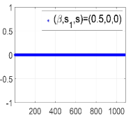
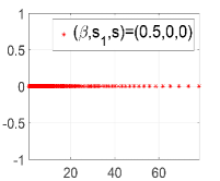
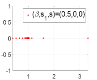
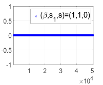
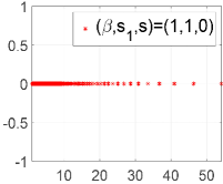
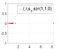
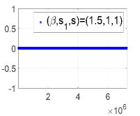
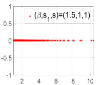
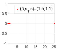
Figure 1: Eigenvalue distribution of the systems (57) or (92) in Example 4.1 with $J=13$ and $\lambda=3$. First column: without preconditioning; second column: preconditioned with the ichol factorization; third column: preconditioned with the T. Chan circulant matrix. The horizontal and vertical axes are respectively the real and imaginary axis.

Example 4.2.

Consider model (3) in $\Omega=(0,1)$ with the boundary condition

$$g(x)=(-2x)\chi_{[-\frac{1}{2},0]}+(2x-2)\chi_{[1,\frac{3}{2}]}$$ (131)

and source term $f(x)$ being derived from the exact solution

$$p(x)=(-2x)\chi_{[-\frac{1}{2},0]}+(x-x^{2})^{2}\chi_{(0,1)}+(2x-2)\chi_{[1,\frac{3}{2}]}.$$ (132)

Obviously, $u(x)$ is discontinuous at $x=\frac{3}{2}$ and $x=-\frac{1}{2}$. In the numerical simulation, for $\lambda=0$, the $f(x_{i}),\,d_{1}(i),\,d_{2}(i)$ are obtained exactly; for $\lambda\not=0$, they are calculated numerically with the techniques as in Example 4.1. The numerical results are listed in Table 4. Since $u(x)$ is smooth enough on $\bar{\Omega}$, the convergence rates are consistent with the theoretical predictions in Theorems 2.3 and 3.1. In fact, for $\lambda=0$ and $\beta\in(1,2)$, the numerical schemes obtained with $s_{1}=s=1$ seem to have a slightly bigger convergence rate than $3-\beta$.

Table 4: Errors and convergence rates in Example 4.2 with $M=2^{J}$, solved by the PCG method with T. Chan’s preconditioner.

$(\beta,\,s,\,s_{1})$	$J$	$\lambda=0$					$\lambda=3$
		$L^{2}$-Err	Rate	$L^{\infty}$-Err	rate	iter	$L^{2}$-Err	Rate	$L^{\infty}$-Err	Rate	iter
	$11$	1.1146e-06	–	1.6944e-06	–	8	5.9414e-06	–	9.6168e-06	–	9
$(0.5,\,0,\,0)$	$12$	3.9593e-07	1.49	6.0100e-07	1.50	8	2.1173e-06	1.49	3.4273e-06	1.49	9
	$13$	1.4043e-07	1.50	2.1297e-07	1.50	8	7.5274e-07	1.49	1.2185e-06	1.49	10
	$11$	4.5687e-09	–	6.7988e-09	–	8	4.8132e-08	–	7.1820e-08	–	9
$(0.5,\,1,\,1)$	$12$	1.1421e-09	2,00	1.6999e-09	2.01	8	1.2059e-08	2.00	1.7999e-08	2.00	9
	$13$	2.8551e-10	2.00	4.2566e-10	2.01	8	3.0193e-09	2.00	4.5084e-09	2.00	9
	$11$	3.7770e-06	–	6.2802e-06	–	12	4.5179e-05	–	6.3557e-05	–	13
$(1.0,\,1,\,0)$	$12$	1.8917e-06	1.00	3.1450e-06	1.00	12	22.2684e-05	0.99	3.1930e-05	0.99	13
	$13$	9.4664e-07	1.00	1.5737e-06	1.00	13	1.1368e-05	1.00	1.6007e-05	1.00	14
	$11$	9.4496e-09	–	51.3552e-08	–	12	1.6933e-07	–	2.6506e-07	–	13
	$12$	2.3615e-09	2.13	3.3872e-09	2.13	12	4.5438e-08	2.02	7.1225e-08	2.02	13
$(1.0,\,1,1)$	$13$	5.9040e-10	2.12	8.4681e-10	2.12	13	1.2138e-08	2.02	1.9048e-08	2.02	14
	$11$	5.5961e-05	–	9.0153e-05	–	19	9.7334e-05	–	1.5346e-04	–	20
	$12$	3.9590e-05	0.50	6.3783e-05	0.50	21	6.9986e-05	0.48	1.1035e-04	0.48	22
$(1.5,\,1,\,0)$	$13$	2.8003e-05	0.50	4.5116e-05	0.50	24	4.9910e-05	0.49	7.8692e-05	0.49	25
	$10$	6.2783e-08	–	8.7275e-08	–	16	—	–	–	–	–
	$11$	1.5532e-08	2.01	2.1605e-08	2.01	19	2.3015e-06	1.49	3.6244e-06	–	20
$(1.5,\,1,\,1)$	$12$	3.8558e-09	2.01	5.3661e-09	2.01	21	8.1576e-07	1.50	1.2851e-06	1.50	23
	$13$	9.5433e-10	2.01	1.3282e-09	2.01	24	2.8888e-07	1.50	4.5524e-07	1.50	25

Example 4.3.

Consider model (3) in $\Omega=(-r,r)$ with source term $f(x)=1$ and absorbing boundary condition $g(x)=0$.

When $\lambda=0$, the exact solution is [9, Subsection 3.1]

$$u(x)=\frac{\sqrt{\pi}(r^{2}-x^{2})^{\beta/2}}{2^{\beta}\Gamma(1+\beta/2)\Gamma(1/2+\beta/2)}~{}~{}~{}{\rm for}~{}x\in\Omega.$$ (133)

It is easy to see that $u(x)$ has a poor regularity at the boundaries of $\Omega$. When $\lambda\not=0$, $u(x)$ cannot be obtained explicitly; the errors (i.e., the data under $\tilde{L}^{2}$-Err and ${\tilde{L}}^{\infty}$-Err) under stepsize $h$ in Table 5 with the $L^{2}$ and $L^{\infty}$ norms are, respectively,

$$\left\|U_{h/2}-U_{h}\right\|~{}~{}{\rm and}~{}~{}\max_{1\leq i\leq M}\left|U_{h/2}-U_{h}\right|,$$ (134)

and the convergence rates are measured by using there errors, where $h=\frac{2r}{M+1}$ with $M=2^{J}-1$. The numerical results in Table 5 show that the convergence rates are small for two cases, being consistent with the results in [29, Example 2].

In statistical physics, the solution $u(x)$ denotes the mean first exit time of a particle starting at $x$ away from the given domain $\Omega$ [8, 11]. For $\lambda=0,\,0.5$ and $3$, the numerical solutions obtained with $(s,s_{1})=(1,1)$ and different values of $\beta=0.5,\,1,\,1.5,\,r=1,\,2,\,5$ are listed in Figures 2, which show: for the same domain $\Omega$, the mean first exit time increases with the increases of the value of $\lambda$; and when $\lambda>0$, for any fixed value of the starting point $x$, the mean exit times are shorter for larger values of $\beta$.

Table 5: Errors and convergence rates in Example 4.3 with $M=2^{J}-1$, solved by the PCG method with T. Chan’s preconditioner. The data in the parentheses denote the rates obtained with the errors in (134).

		$\lambda=0$				$\lambda=3$
$(\beta,\,s,\,s_{1})$	$M$	$L^{2}$-Err	Rates	${L}^{\infty}$-Err	rates	$\tilde{L}^{2}$-Err	Rate	${\tilde{L}}^{\infty}$-Err	rate
	$11$	3.5668e-03	–	5.4682e-02	–	3.3886e-02	–	2.2117e-01	–
$(0.5,\,0,\,0)$	$12$	2.1205e-03	0.75 (0.75)	4.5975e-02	0.25 (0.25)	1.6834e-02	1.01	1.8113e-01	0.29
	$13$	1.2608e-03	0.75 (0.75)	3.8658e-02	0.25 (0.25)	8.5734e-03	0.97	1.4951e-01	0.28
	$11$	1.4675e-03	–	2.0163e-02	–	1.3158e-02	–	8.0461e-02	–
$(0.5,\,1,\,1)$	$12$	8.7272e-04	0.75 (0.75)	1.6952e-02	0.25 (0.25)	6.9321e-03	0.92	6.5320e-02	0.30
	$13$	5.1896e-04	0.75 (0.75)	1.4254e-02	0.25 (0.25)	3.6595e-03	0.92	5.3565e-02	0.29
	$11$	6.3631e-04	–	4.7004e-03	–	1.6940e-03	–	6.1020e-03	–
$(1.0,\,1,\,0)$	$12$	3.3183e-04	0.94 (0.94)	3.3232e-03	0.50 (0.50)	8.7755e-04	0.95	4.2848e-03	0.51
	$13$	1.7249e-04	0.94 (0.94)	2.3497e-03	0.50 (0.50)	4.4946e-04	0.97	3.0161e-03	0.51
	$11$	6.3631e-04	–	4.7004e-03	–	1.6940e-03	–	6.1020e-03	–
$(1.0,\,1,\,1)$	$12$	3.3183e-04	1.08 (1.08)	3.3232e-03	0.64 (0.64)	8.7755e-04	1.09	4.2848e-03	0.65
	$13$	1.7249e-04	1.07 (1.07)	2.3497e-03	0.63 (0.63)	4.4946e-04	1.09	3.0161e-03	0.63
	$11$	1.6135e-03	–	1.3157e-03	–	2.7348e-03	–	2.4835e-03	–
$(1.5\,\,1,\,0)$	$12$	1.1034e-03	0.55 (0.58)	9.0676e-04	(0.54)  (0.56)	1.9986e-03	0.45	1.8304e-03	0.44
	$13$	7.6158e-04	0.53 (0.56)	6.2939e-04	(0.53)  (0.54)	1.4278e-03	0.49	1.3146e-03	0.48
	$11$	2.2426e-04	–	5.4375e-04	–	1.8108e-04	–	5.7640e-04	–
$(1.5,\,1,\,1)$	$12$	1.1260e-04	0.99 (0.99)	3.2327e-04	0.75 (0.75)	1.1576e-04	0.65	3.4404e-04	0.74
	$13$	5.6465e-05	1.00 (1.00)	1.9220e-04	0.75 (0.75)	6.9126e-05	0.74	2.0489e-04	0.75

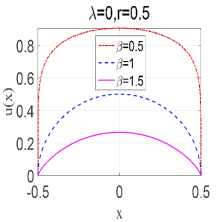
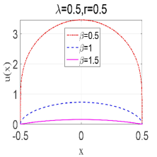
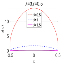
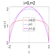
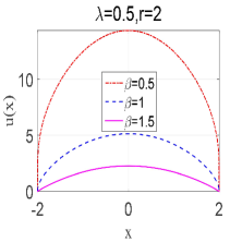
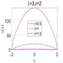
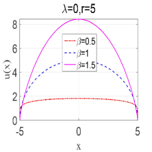
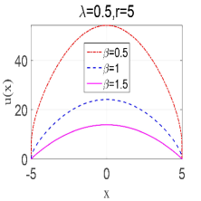
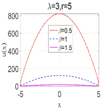
Figure 2: Dependence of the mean exit time $u(x)$ on the size of domain $\Omega$, and the values of $\beta$ and $\lambda$.

5 Conclusion

The tempered fractional Laplacian is a recently introduced operator for treating the weaknesses of the fractional Laplacian in some physical processes. This paper provides several classes of finite difference schemes for the tempered fractional Laplacian equation with $\beta\in(0,2)$. According to the regularity of the solution, one can choose the more appropriate numerical schemes. The detailed numerical analyses are performed, and the effective preconditioning techniques are provided. The implementation details are also discussed, including that the entries of the stiffness matrix can be explicitly and conveniently calculated and the stiffness matrix has Toeplitz-like structure. The efficiencies of the algorithms are verified by extensive numerical experiments and the desired convergence rates are confirmed.

References

- [1] M. Abramowitz and I. A. Stegun, Handbook of Mathematical Functions, Dover Publications, 1965, Chapter 5.
- [2] G. Acosta and J. P. Borthagaray, A fractional Laplace equation: regularity of solutions and finite element approximations, SIAM J. Numer. Anal., 55 (2017), pp. 472-495.
- [3] Advanpix Multiprecision Computing Toolbox for MATLAB, http://www.advanpix.com/, accessed 2017-10-24.
- [4] D. Applebaum, Lévy Process and Stochastic Calculus, 2nd ed., Cambridge University Press, Cambridge, UK, 2009.
- [5] O. Axelssion, Iterative Solution Methods, Cambridge University press, UK, 1996.
- [6] B. Baeumer and M. M. Meerschaert, Tempered stable Lévy motion and transient supper-diffusion, J. Comput. Appl. Math., 233 (2010), pp. 2438-2448.
- [7] R. H. Chan and X. Q. Jin, An Introduction to Iterative Teoplitz Solvers, SIAM, 2007.
- [8] W. H. Deng, X. C. Wu, and W. L. Wang, Mean exit time and escape probability for the anomalous processes with the tempered power-law waiting times, EPL, 117 (2016).
- [9] W. H. Deng, B. Y. Li, W. Y. Tian, and P. W. Zhang, Boundary problems for the fractional and tempered fractional operators, Multiscale Model. Simul., in press, 2017.
- [10] T. Gao, J. Duan, X. Li, and R. Song, Mean exit time and escape probabilty for dynamical systems driven by Lévy noises, SIAM J. Sci, Comput., 36 (2014), pp. A887-A906.
- [11] R. K. Getoor, First passage times for symmetric stable processes in space, Trans. Amer. Math. Soc., 101 (1961), pp. 75-90.
- [12] I. S. Gradshteyn, I. M. Ryzhik, Y. V. Geraniums, and M. Y. Tseytlin, Table of Integrals, Series, and Products, A. Jeffrey, ed., Translated by Scripta Technica, Academic Press, USA, 1980.
- [13] J. S. Hesthaven and T. Warburton, Nodal Discontinuous Galerkin Methods: Algorithms, Analysis, and Applications, Springer, Berlin, 2008.
- [14] J. F. Huang, Y. F. Tang, and L. Vázquez, Convergence analysis of a block-by-block method for fractional differential equations, Numer. Math. Theor. Meth. Appl. 5 (2012), pp. 229-241.
- [15] Y. H. Huang and A. Oberman, Numerical methods for the fractional Laplacian: a finite difference-quadrature approach, SIAM. J. Numer. Anal. 52 (2014), pp. 3056-3084.
- [16] J. H. Jia and H. Wang, Fast finite difference methods for space-fractional diffusion equations with fractional derivative boundary conditions, J. Comput. Phys., 293 (2015), pp. 359-369.
- [17] S. L. Lei and H. W. sun, A circulant preconditioner for fractional diffusion equations, J. Comput. Phys., 242 (2013), 715-725.
- [18] C. Li and W. H. Deng, High order schemes for the tempered fractional diffusion equations, Adv. Comput. Math., 42 (2016), pp. 543–572.
- [19] F. R. Lin, S. W. Yang, and X. Q. Jin, Preconditioned iterative methods for fractional diffusion equation, J. Comput. Phys., 256 (2014), pp. 109-117.
- [20] M. M. Meerschaert and C. Tadjeran, Finite difference approximations for fractional advection-dispersion flow equations, J. Comput. Appl. Math., 172 (2004), pp. 65-77.
- [21] J. Y. Pan, R. Ke, M. K. NG, and H. W. Sun, Precondtioing techniques for diagonal-times-Toeplitz matrices in fractional diffusion equations, SIAM J. Sci. Comput., 36 (2014), pp. A2698-A2719.
- [22] S. Peszat and J. Zabczyk, Stochastic Partial Differential Equations with Lévy Processes, Cambridge University Press, Cambridge, UK, 2007.
- [23] C. Pozrikidis, The Fractional Laplacian, CRC Press, London, 2016.
- [24] F. Sabzikar, M. M. Meerschaert, and J. H. Chen, Tempered fractional calculus, J. Comput. Phys., 293 (2015), pp. 14-28.
- [25] J. Shen, T. Tang, and L. L, Wang, Spectral Methods: Algorithms, Analysis and Applications, Springer, New York, 2011.
- [26] C. T. Sheng and J. Shen, A hybrid spectral element method for fractional two-point boundary value problems, Numer. Math. Theor. Meth. Appl. 10 (2017), pp. 437-464.
- [27] Q. Yang, F. Liu, and I. Turner, Numerical methods for fractional partial differential equations with Riesz space fractional derivatives, Appl. Math. Model., 34 (2010), pp. 200-218.
- [28] V. Zaburdaev, S. Denisov, and J. Klafter, Lévy walks, Rev. Modern Phys., 87 (2015), pp. 483-530.
- [29] Z. J. Zhang, W. H. Deng, and G. E. Karniadakis, A Riesz basis Galerkin method for the tempered fractional Laplacian, arXiv:1709.10415, 2017.
- [30] Z. Zhao, X. Q. Jin, and M. M. Lin, Preconditioned iterative methods for space-time fractional advection-diffusion equations, J. Comput. Phys., 319 (2016), pp. 266-279.
- [31] X. Zhao, Z. Z. Sun, and Z. H. Hao, A fourth-order compact ADI scheme for two-dimensional nonlinear space fractional Schrödinger equation, SIAM J. Sci. Comput., 36 (2014), pp. A2865-A2886.