Abstract

We present a detailed theoretical analysis of the problem of multiple-source adaptation in the general stochastic scenario, extending known results that assume a single target labeling function. Our results cover a more realistic scenario and show the existence of a single robust predictor accurate for any target mixture of the source distributions. Moreover, we present an efficient and practical optimization solution to determine the robust predictor in the important case of squared loss, by casting the problem as an instance of DC-programming. We report the results of experiments with both an artificial task and a sentiment analysis task. We find that our algorithm outperforms competing approaches by producing a single robust model that performs well on any target mixture distribution.

1 Introduction

In many modern applications, often the learner has access to information about several source domains, including accurate predictors possibly trained and made available by others, but no direct information about a target domain for which one wishes to achieve a good performance. The target domain can typically be viewed as a combination of the source domains, that is a mixture of their joint distributions, or it may be close to such mixtures.

Such problems arise commonly in speech recognition where different groups of speakers (domains) yield different acoustic models and the problem is to derive an accurate acoustic model for a broader population that may be viewed as a mixture of the source groups Liao (2013). In visual recognition multiple image databases exist each with its own bias and labeled categories Torralba and Efros (2011), but the target application may contain some combination of image types and any category may need to be recognized. Finally, in sentiment analysis accurate predictors may be available for sub-domains such as TVs, laptops and CD players for which labeled training data was at the learner’s disposal, but not for the more general category of electronics, which can be modeled as a mixture of the sub-domains (Blitzer et al., 2007; Dredze et al., 2008).

Many have considered the case of transferring between a single source and known target domain either through unsupervised adaptation (no labels in the target) techniques (Gong et al., 2012; Long et al., 2015; Ganin and Lempitsky, 2015; Tzeng et al., 2015) or supervised (some labels in the target) (Saenko et al., 2010; Yang et al., 2007; Hoffman et al., 2013; Girshick et al., 2014).

Here, we focus on the case of multiple source domains and ask how the learner can combine relatively accurate predictors available for source domains to derive an accurate predictor for any new mixture target domain. This is known as the multiple-source adaption problem first formalized and analyzed theoretically by Mansour et al. (2008, 2009) and later studied for various applications such as object recognition (Hoffman et al., 2012; Gong et al., 2013a, b). In the most general setting, even unlabeled information may not be available about the target domain, though one can expect it to be a mixture of the source distributions. Thus, the problem is also closely related to domain generalization (Pan and Yang, 2010; Muandet et al., 2013; Xu et al., 2014), where knowledge from an arbitrary number of related domains is combined to perform well on a previously unseen domain. Several algorithms have been proposed based on convex combinations of predictors from multiple source domains (Schweikert et al., 2009; Chattopadhyay et al., 2012; Duan et al., 2012a, b).

We build on the work of Mansour et al. (2008), which proved that a distribution weighted predictor admits a small loss on any target mixture for the special case of deterministic predictors, however the algorithmic problem of finding such a weighting was left as a difficult question since it required solving a Brouwer fixed-point problem.

The first main contribution of this work is extending the multiple-source adaptation theory from deterministic true predictors to stochastic ones, that is the scenario where there is a distribution over the joint feature and label space, $\mathcal{X}\times\mathcal{Y}$, as opposed to deterministic case where a unique target labeling function is assumed. This generalization is needed to cover the realistic cases in applications. Under the assumption that the conditional distributions are the same for all domains, our analysis shows that for the stochastic scenario there exists a robust predictor that admits a small expected loss with respect to any mixture distribution. We further extend this result to an arbitrary distribution with small Rényi divergence with respect to the family of mixtures. We also extend it to the case where, instead of having access to the ideal distributions, only estimate distributions are used for deriving that hypothesis. Finally, we present a novel extension of the theory not covered by Mansour et al. (2008, 2009), to the more realistic case where the conditional distributions are distinct.

Our second main contribution is a new formulation of the problem of finding that robust predictor. Note again that no algorithm was previously given by Mansour et al. (2008) for this problem (for their experiments they directly used the target mixture weights). We show that, in the important case of the squared loss, the problem can be cast as a DC-programming problem and we present an efficient and practical optimization solution for it. We have fully implemented our algorithm and report the results of experiments with both an artificial task and a sentiment analysis task. We find that our algorithm outperforms competing approaches by producing a single robust model that performs well on any target mixture distribution.

2 Problem set-up

We consider a multiple-source domain adaptation problem in the general stochastic scenario where there is a distribution over $\mathcal{X}\times\mathcal{Y}$, as opposed to the special case where a target function mapping from $\mathcal{X}$ to $\mathcal{Y}$ is assumed (deterministic scenario) (Mansour et al., 2008). This extension is needed for the analysis of the most common and realistic learning set-ups in practice.

Let $\mathcal{X}$ denote the input space and $\mathcal{Y}$ the output space. We will identify a domain with a distribution over $\mathcal{X}\times\mathcal{Y}$ and consider the scenario where the learner has access to a predictor $h_{k}\colon\mathcal{X}\to\mathcal{Y}$, for each domain ${\mathscr{D}}_{k}$, $k=1,\ldots,p$. The learner’s objective is to combine these predictors so as to minimize error for a target domain that may be mixture of the source domains, or close to such mixtures.

In order to find such a good combination, the learner also needs access to ${\mathscr{D}}_{k}(x,y)$ or a good estimate $\widehat{\mathscr{D}}_{k}(x,y)$. In fact, in practice the learner would rarely have access to ${\mathscr{D}}_{k}$, but only $\widehat{\mathscr{D}}_{k}$. Note that, even though $h^{*}(x)=\sum_{y}y{\mathscr{D}}_{k}(x,y)$ is the optimal predictor under the squared loss for domain $k$, $\sum_{y}y\widehat{\mathscr{D}}_{k}(x,y)$ may have a poor generalization performance and not form a good predictor.

Much of our theory applies to an arbitrary loss function $L\colon\mathcal{Y}\times\mathcal{Y}\to\mathbb{R}_{+}$ that is convex and continuous. We will denote by $\mathcal{L}({\mathscr{D}},h)$ the expected loss of a predictor $h\colon\mathcal{X}\to\mathcal{Y}$ with respect to the distribution ${\mathscr{D}}$:

$$\mathcal{L}({\mathscr{D}},h) = \operatorname*{\mathbb{E}}_{(x,y)\sim{\mathscr{D}}}\big{[}L(h(x),y)\big{]}$$ (1)

$$= \sum_{(x,y)\in\mathcal{X}\times\mathcal{Y}}{\mathscr{D}}(x,y)L(h(x),y).$$

But, we will be particularly interested in the case where $L$ is the squared loss, that is $L(h(x),y)=(h(x)-y)^{2}$.

We will assume that each $h_{k}$ is a relatively accurate predictor for the distribution ${\mathscr{D}}_{k}$ and that there exists $\epsilon>0$ such that $\mathcal{L}({\mathscr{D}}_{k},h_{k})\leq\epsilon$ for all $k\in[1,p]$. We will first assume that the conditional probability of the output labels is the same for all source domains, that is, for any $(x,y)$, ${\mathscr{D}}_{k}(y|x)$ does not depend on $k$. This is a natural assumption that is more general than the one adopted by Mansour et al. (2008) in the analysis of the deterministic scenario where exactly the same labeling function $f$ is assumed for all source domains. We then relax this requirement later and provide guarantees for distinct conditional probabilities.

We will also assume that the average loss of the source predictors under the uniform distribution ${\mathscr{U}}^{1}$ over $\mathcal{X}$ is bounded, that is, there exists $M\geq 0$ such that

$$\frac{1}{p}\sum_{k=1}^{p}\sum_{(x,y)\in\mathcal{X}\times\mathcal{Y}}\mathcal{D}_{k}(y|x){\mathscr{U}}^{1}(x)L(h_{k}(x),y)\leq M.$$

3 Theoretical analysis

In this section, we present a theoretical analysis of the general multiple-source adaptation in stochastic case.

We first show that when the conditional distributions ${\mathscr{D}}_{k}(y|x)$ are the same for all source domains, there exists a single weighted combination rule $h_{z}^{\eta}$ that admits a small loss with respect to any target mixture distribution ${\mathscr{D}}_{\lambda}$, that is any $\lambda$ (Section 3.1). We further give guarantees for the loss of that hypothesis with respect to an arbitrary distribution ${\mathscr{D}}_{T}$ (Section 3.2). Next, we extend our guarantees to the case where the source distributions ${\mathscr{D}}_{k}$ are not directly accessible and where the weighted combination rule is derived using estimates of the distributions ${\mathscr{D}}_{k}$ (Section 3.3). Finally, we provide guarantees for the most general case where the conditional distributions ${\mathscr{D}}_{k}(y|x)$ are distinct and for an arbitrary target distribution ${\mathscr{D}}_{T}$ (Section 3.4).

3.1 Mixture target distribution

Here we consider the case of a target distribution, that is a mixture distribution ${\mathscr{D}}_{\lambda}=\sum_{k=1}^{p}\lambda_{k}{\mathscr{D}}_{k}$, for some $\lambda=(\lambda_{1},\ldots,\lambda_{p})$ in the simplex $\Delta=\{\lambda\in\mathbb{R}^{p}\colon\forall k\in[p],\lambda_{k}\geq 0,\sum_{k=1}^{p}\lambda_{k}=1\}$. The mixture weight $\lambda\in\Delta$ defining ${\mathscr{D}}$ is not known to us. Thus, our objective will be to find a hypothesis with small loss with respect to any mixture distribution ${\mathscr{D}}_{\lambda}$, using a combination of trained domain-specific hypotheses $h_{k}$s.

Extending the definition given by Mansour et al. (2008), we define the distribution-weighted combination of the models $h_{k}$, $k\in[1,p]$ as follows. For any $z\in\Delta$, $\eta>0$, and $x\in\mathcal{X}$,

$$h_{z}^{\eta}(x) =\mspace{-5.0mu}\sum_{k=1}^{p}\sum_{y\in\mathcal{Y}}\frac{z_{k}{\mathscr{D}}_{k}(x,y)+\eta\frac{{\mathscr{U}}(x,y)}{p}}{\sum_{k=1}^{p}\sum_{y\in\mathcal{Y}}z_{k}{\mathscr{D}}_{k}(x,y)+\eta{\mathscr{U}}(x,y)}h_{k}(x)$$ (2)

$$=\sum_{k=1}^{p}\frac{z_{k}{\mathscr{D}}^{1}_{k}(x)+\eta\frac{{\mathscr{U}}^{1}(x)}{p}}{\sum_{k=1}^{p}z_{k}{\mathscr{D}}^{1}_{k}(x)+\eta{\mathscr{U}}^{1}(x)}h_{k}(x),$$ (3)

where ${\mathscr{U}}$ is the uniform distribution over $\mathcal{X}\times\mathcal{Y}$, and where, we denote by ${\mathscr{D}}^{1}(x)$ the marginal distribution over $\mathcal{X}$: ${\mathscr{D}}^{1}(x)=\sum_{y\in\mathcal{Y}}{\mathscr{D}}(x,y)$.

The distribution weighted combination is the natural ensemble solution in the case where the models $h_{k}$s have been trained with different distributions. In fact, when ${\mathscr{D}}_{k}$s coincide, $h_{z}$ is the standard convex ensemble of the $h_{k}$s.

Observe that for any $x\in\mathcal{X}$, $h^{\eta}_{z}(x)$ is continuous in $z$ since the denominator in (2) is positive ($\eta>0$). By the continuity of $L$, this implies that, for any distribution ${\mathscr{D}}$, $\mathcal{L}({\mathscr{D}},h_{z}^{\eta})$ is continuous in $z$.

Our proof makes use of the following Fixed Point Theorem of Brouwer.

Theorem 1.

For any compact and convex non-empty set $C\subset\mathbb{R}^{p}$ and any continuous function $f\colon C\rightarrow C$, there is a point $x\in C$ such that $f(x)=x$.

Lemma 2.

For any $\eta,\eta^{\prime}>0$, there exists $z\in\Delta$, with $z_{k}\neq 0$ for all $k\in[1,p]$, such that the following holds for the distribution weighted combining rule $h_{z}^{\eta}$:

$$\forall k\in[p],\quad\mathcal{L}({\mathscr{D}}_{k},h_{z}^{\eta})\leq\sum_{j=1}^{p}z_{j}\mathcal{L}({\mathscr{D}}_{j},h_{z}^{\eta})+\eta^{\prime}.$$ (4)

Proof.

Consider the mapping $\Phi\colon\Delta\to\Delta$ defined for all $z\in\Delta$ by

$$[\Phi(z)]_{k}=\frac{z_{k}\,\mathcal{L}({\mathscr{D}}_{k},h_{z}^{\eta})+\frac{\eta^{\prime}}{p}}{\sum_{j=1}^{p}z_{j}\mathcal{L}({\mathscr{D}}_{j},h_{z}^{\eta})+\eta^{\prime}}.$$

$\Phi$ is continuous since $\mathcal{L}({\mathscr{D}}_{k},h_{z}^{\eta})$ is a continuous function of $z$ and since the denominator is positive ($\eta^{\prime}>0$). Thus, by Brouwer’s Fixed Point Theorem, there exists $z\in\Delta$ such that $\Phi(z)=z$. For that $z$, we can write

$$z_{k}=\frac{z_{k}\,\mathcal{L}({\mathscr{D}}_{k},h_{z}^{\eta})+\frac{\eta^{\prime}}{p}}{\sum_{j=1}^{p}z_{j}\mathcal{L}({\mathscr{D}}_{j},h_{z}^{\eta})+\eta^{\prime}},$$

for all $k\in[1,p]$. Since $\eta^{\prime}$ is positive, we must have $z_{k}\neq 0$ for all $k$. Dividing both sides by $z_{k}$ gives $\mathcal{L}({\mathscr{D}}_{k},h_{z}^{\eta})=\sum_{j=1}^{p}z_{j}\mathcal{L}({\mathscr{D}}_{j},h_{z}^{\eta})+\eta^{\prime}-\frac{\eta^{\prime}}{pz_{k}}\leq\sum_{j=1}^{p}z_{j}\mathcal{L}({\mathscr{D}}_{j},h_{z}^{\eta})+\eta^{\prime}$, which completes the proof. ∎

Theorem 3.

For any $\delta>0$, there exists $\eta>0$ and $z\in\Delta$, such that $\mathcal{L}({\mathscr{D}}_{\lambda},h_{z}^{\eta})\leq\epsilon+\delta$  for any mixture parameter $\lambda\in\Delta$.

The proof uses the convexity of the loss function and Lemma 2. The full proof is given in the supplementary. The theorem shows the existence of a mixture weight $z\in\Delta$ and $\eta>0$ with a remarkable property: for any $\delta>0$, regardless of which mixture weight $\lambda\in\Delta$ defines the target distribution, the loss of $h_{z}^{\eta}$ is at most $\epsilon+\delta$, that is arbitrarily close to $\epsilon$. $h_{z}^{\eta}$ is therefore a robust hypothesis with a favorable property for any mixture target distribution. More precisely, by the proof of the theorem, for any $z\in\Delta$ verifying (4), $h_{z}^{\eta}$ admits this property. We exploit this in the next section to devise an algorithm for finding such a $z\in\Delta$.

3.2 Arbitrary target distribution

Here, we extend the results of the previous section to the case of an arbitrary target distribution ${\mathscr{D}}_{T}$ that may not be a mixture of the source distributions, by extending the results of Mansour, Mohri, and Rostamizadeh (2009).

We will assume that the loss of the source hypotheses $h_{k}$ is bounded, that is $L(h_{k}(x),y)\leq M$ for all $(x,y)\in\mathcal{X}\times\mathcal{Y}$. By convexity, this immediately implies that for any distribution combination hypothesis $h_{z}^{\eta}$,

$$L(h_{z}^{\eta}(x),y) \leq\sum_{k=1}^{p}\frac{z_{k}{\mathscr{D}}^{1}_{k}(x)+\eta\frac{{\mathscr{U}}^{1}(x)}{p}}{{\mathscr{D}}^{1}_{z}(x)+\eta{\mathscr{U}}^{1}(x)}L\big{(}h_{k}(x),y\big{)}$$

$$\leq\sum_{k=1}^{p}\frac{z_{k}{\mathscr{D}}^{1}_{k}(x)+\eta\frac{{\mathscr{U}}^{1}(x)}{p}}{{\mathscr{D}}^{1}_{z}(x)+\eta{\mathscr{U}}^{1}(x)}M=M.$$

Our extension to an arbitrary target distribution ${\mathscr{D}}_{T}$ is based on the divergence of ${\mathscr{D}}_{T}$ from the family of all mixtures of the source distributions ${\mathscr{D}}_{k}$, $k\in[p]$. Different divergence measures could be used in this context. The one that naturally comes up in our analysis as in previous work, is the Rényi Divergence (Rényi, 1961). The Rényi Divergence is parameterized by $\alpha$ and denote by ${\mathsf{D}}_{\alpha}$. The $\alpha$-Rényi Divergence of two distributions ${\mathscr{D}}$ and ${\mathscr{D}}^{\prime}$ is defined by

$${\mathsf{D}}_{\alpha}({\mathscr{D}}\parallel{\mathscr{D}}^{\prime})=\frac{1}{\alpha-1}\log\mspace{-20.0mu}\sum_{(x,y)\in\mathcal{X}\times\mathcal{Y}}\mspace{-25.0mu}{\mathscr{D}}(x,y)\left[\frac{{\mathscr{D}}(x,y)}{{\mathscr{D}}^{\prime}(x,y)}\right]^{\alpha-1}\mspace{-25.0mu}.$$ (5)

It can be shown that the Rényi Divergence is always non-negative and that for any $\alpha>0$, ${\mathsf{D}}_{\alpha}({\mathscr{D}}\parallel{\mathscr{D}}^{\prime})=0$ iff ${\mathscr{D}}={\mathscr{D}}^{\prime}$, (see Arndt (2004)). The Rényi divergence coincides with the following known measure for some specific values of $\alpha$:

• $\alpha=1$: ${\mathsf{D}}_{1}({\mathscr{D}}\parallel{\mathscr{D}}^{\prime})$ coincides with the standard relative entropy or KL-divergence.

• $\alpha=2$: ${\mathsf{D}}_{2}({\mathscr{D}}\parallel{\mathscr{D}}^{\prime})=\log\operatorname*{\mathbb{E}}_{(x,y)\sim{\mathscr{D}}}\big{[}\frac{{\mathscr{D}}(x,y)}{{\mathscr{D}}^{\prime}(x,y)}\big{]}$ is the logarithm of the expected probabilities ratio.

• $\alpha=+\infty$: ${\mathsf{D}}_{\infty}({\mathscr{D}}\parallel{\mathscr{D}}^{\prime})=\log\displaystyle\sup_{(x,y)\in\mathcal{X}\times\mathcal{Y}}\textstyle\big{[}\frac{{\mathscr{D}}(x,y)}{{\mathscr{D}}^{\prime}(x,y)}\big{]}$, which bounds the maximum ratio between two probability distributions.

We will denote by ${\mathsf{d}}_{\alpha}({\mathscr{D}}\parallel{\mathscr{D}}^{\prime})$ the exponential:

$$\mspace{-1.0mu}{\mathsf{d}}_{\alpha}({\mathscr{D}}\parallel{\mathscr{D}}^{\prime})=e^{{\mathsf{D}}_{\alpha}({\mathscr{D}}\parallel{\mathscr{D}}^{\prime})}\mspace{-6.0mu}=\mspace{-4.0mu}\left[\mspace{-2.0mu}\sum_{(x,y)\in\mathcal{X}\times\mathcal{Y}}\frac{{\mathscr{D}}^{\alpha}(x,y)}{{\mathscr{D}}^{\prime\alpha-1}(x,y)}\right]^{\frac{1}{\alpha-1}}\mspace{-35.0mu}.\mspace{-15.0mu}$$ (6)

Given a class of distributions $\mathcal{D}$, we denote by ${\mathsf{D}}_{\alpha}({\mathscr{D}}\parallel{\mathcal{D}})$ the infimum $\inf_{{\mathscr{D}}^{\prime}\in{\mathcal{D}}}{\mathsf{D}}_{\alpha}({\mathscr{D}}\parallel{\mathscr{D}}^{\prime})$. We will concentrate on the case where $\mathcal{D}$ is the class of all mixture distributions over a set of $k$ source distributions, i.e., ${\mathcal{D}}=\{{\mathscr{D}}_{\lambda}\colon{\mathscr{D}}_{\lambda}=\sum_{k=1}^{p}\lambda_{k}{\mathscr{D}}_{k},\lambda\in\Delta\}$.

Theorem 4.

Let ${\mathscr{D}}_{T}$ be an arbitrary target distribution. For any $\delta>0$, there exists $\eta>0$ and $z\in\Delta$, such that the following inequality holds for any $\alpha>1$:

$$\mathcal{L}({\mathscr{D}}_{T},h_{z}^{\eta})\leq\Big{[}(\epsilon+\delta)\,{\mathsf{d}}_{\alpha}({\mathscr{D}}_{T}\parallel\mathcal{D})\Big{]}^{\frac{\alpha-1}{\alpha}}M^{\frac{1}{\alpha}}.$$

The proof of Theorem 4 is given in the supplementary. Note that in the particular case where ${\mathscr{D}}_{T}$ is in $\mathcal{D}$, we have ${\mathsf{d}}_{\alpha}({\mathscr{D}}_{T}\parallel\mathcal{D})=1$. For $\alpha\to+\infty$, we then retrieve the result of Theorem 3.

3.3 Arbitrary target distribution and estimate distributions

We now further extend our analysis to the case where the distributions ${\mathscr{D}}_{k}$ are not directly available to the learner and where instead estimates $\widehat{\mathscr{D}}_{k}$ have been derived from data.

For $k\in[p]$, let $\widehat{\mathscr{D}}_{k}$ be an estimate of ${\mathscr{D}}_{k}$ and define $\widehat{\epsilon}$ by

$$\widehat{\epsilon}=\max_{k\in[p]}\Big{[}\epsilon\,{\mathsf{d}}_{\alpha}(\widehat{\mathscr{D}}_{k}\parallel{\mathscr{D}}_{k})\Big{]}^{\frac{\alpha-1}{\alpha}}M^{\frac{1}{\alpha}}.$$ (7)

Note that when for all $k\in[p]$, $\widehat{\mathscr{D}}_{k}$ is a good estimate of ${\mathscr{D}}_{k}$, then ${\mathsf{d}}_{\alpha}(\widehat{\mathscr{D}}_{k}\parallel{\mathscr{D}}_{k})$ is close to one and, for $\alpha\to+\infty$, $\widehat{\epsilon}$ is very close to $\epsilon$. We will denote by $\widehat{\mathcal{D}}$ the family of mixtures of the estimates $\widehat{\mathcal{D}}_{k}$:

$$\widehat{\mathcal{D}}=\left\{\sum_{k=1}^{p}\lambda_{k}\widehat{\mathscr{D}}_{k}\colon k\in\Delta\right\}.$$ (8)

We will denote by $\widehat{h}_{z}^{\eta}$ the distribution weighted combination hypothesis based on the estimate distributions $\widehat{\mathscr{D}}_{k}$:

$$\widehat{h}_{z}^{\eta}(x)=\sum_{k=1}^{p}\frac{z_{k}\widehat{\mathscr{D}}^{1}_{k}(x)+\eta\,\frac{{\mathscr{U}}^{1}(x)}{p}}{\sum_{j=1}^{p}z_{j}\widehat{\mathscr{D}}^{1}_{j}(x)+\eta{\mathscr{U}}^{1}(x)}h_{k}(x),$$ (9)

where we denote by $\widehat{\mathscr{D}}^{1}(x)$ the marginal distribution over $\mathcal{X}$: $\widehat{\mathscr{D}}^{1}(x)=\sum_{y\in\mathcal{Y}}\widehat{\mathscr{D}}(x,y)$.

Theorem 5.

Let ${\mathscr{D}}_{T}$ be an arbitrary target distribution. Then, for any $\delta>0$, there exists $\eta>0$ and $z\in\Delta$, such that the following inequality holds for any $\alpha>1$:

$$\mathcal{L}({\mathscr{D}}_{T},\widehat{h}_{z}^{\eta})\leq\Big{[}(\widehat{\epsilon}+\delta)\,{\mathsf{d}}_{\alpha}({\mathscr{D}}_{T}\parallel\widehat{\mathcal{D}})\Big{]}^{\frac{\alpha-1}{\alpha}}M^{\frac{1}{\alpha}}.$$

The proof of Theorem 5 depends heavily on the result of Theorem 4, and is given in the supplementary. This result shows that there exists a predictor $\widehat{h}_{z}^{\eta}$ based on the estimate distributions $\widehat{\mathscr{D}}_{k}$ that is $\widehat{\epsilon}$-accurate with respect to any target distribution ${\mathscr{D}}_{T}$ whose Rényi divergence with respect to the family $\widehat{\mathcal{D}}$ is not too large, i.e. ${\mathsf{d}}_{\alpha}({\mathscr{D}}_{T}\parallel\widehat{\mathcal{D}})$ close to $1$. Furthermore, $\widehat{\epsilon}$ is close to $\epsilon$, provided that $\widehat{\mathscr{D}}_{k}$s are good estimates of ${\mathscr{D}}_{k}$s, i.e. ${\mathsf{d}}_{\alpha}(\widehat{\mathscr{D}}_{k}\parallel{\mathscr{D}}_{k})$ close to $1$.

Theorem 5 used the Rényi divergence in both directions: ${\mathsf{d}}_{\alpha}({\mathscr{D}}_{T}\parallel\widehat{\mathcal{D}})$ requires $\text{Supp}({\mathscr{D}}_{T})\subseteq\text{Supp}(\widehat{\mathcal{D}})$, and ${\mathsf{d}}_{\alpha}(\widehat{\mathscr{D}}_{k}\parallel{\mathscr{D}}_{k})$ requires $\text{Supp}(\widehat{\mathscr{D}}_{k})\subseteq\text{Supp}({\mathscr{D}}_{k}),k\in[p]$. Many density estimation methods fulfill these requirements, for instance kernel density estimation, Maxent models, or $n$-gram language models. In our experiments (Section 5), we fit our data using a bigram language model for sentiment analysis.

For any two distributions ${\mathscr{D}},{\mathscr{D}}^{\prime}$, the Rényi divergence (and ${\mathsf{d}}_{\alpha}({\mathscr{D}}\parallel{\mathscr{D}}^{\prime})$) is nondecreasing as a function of $\alpha$, and

$${\mathsf{d}}_{\alpha}({\mathscr{D}}\parallel{\mathscr{D}}^{\prime})\leq{\mathsf{d}}_{\infty}({\mathscr{D}}\parallel{\mathscr{D}}^{\prime})=\sup_{(x,y)\in\mathcal{X}\times\mathcal{Y}}\left[\frac{{\mathscr{D}}(x,y)}{{\mathscr{D}}^{\prime}(x,y)}\right].$$

Thus, it is reasonable to assume that ${\mathsf{d}}_{\alpha}({\mathscr{D}}_{T}\parallel\widehat{\mathcal{D}})$ and ${\mathsf{d}}_{\alpha}(\widehat{\mathscr{D}}_{k}\parallel{\mathscr{D}}_{k}),k\in[p]$ are not too large when $\widehat{\mathscr{D}}_{k}$ are good estimates of ${\mathscr{D}}_{k},k\in[p]$.

3.4 Arbitrary target distribution and distinct conditional probability distributions

This section examines the case where the conditional probability distributions of the source domains are distinct, and the target distribution is arbitrary. This is a novel extension that was not discussed in Mansour et al. (2009).

Let ${\mathscr{D}}_{T}(\cdot|x)$ denote the conditional probability distribution on target domain, and ${\mathscr{D}}_{k}(\cdot|x)$ denote the conditional probability distribution associated to source $k$. ${\mathscr{D}}_{T}(\cdot|x),{\mathscr{D}}_{k}(\cdot|x),k\in[p]$ are not necessarily the same. Define $\epsilon_{T}$ by

$$\epsilon_{T}\mspace{-3.0mu}=\mspace{-3.0mu}\max_{k\in[p]}\Big{[}\mathbb{E}_{{\mathscr{D}}^{1}_{k}(x)}{\mathsf{d}}_{\alpha}\left({\mathscr{D}}_{T}(\cdot|x)\parallel{\mathscr{D}}_{k}(\cdot|x)\right)^{\alpha-1}\Big{]}^{\mspace{-4.0mu}\frac{1}{\alpha}}\mspace{-5.0mu}\epsilon^{\frac{\alpha-1}{\alpha}}\mspace{-5.0mu}M^{\frac{1}{\alpha}}.$$

Therefore, if for every domain $k$, ${\mathscr{D}}_{T}(\cdot|x)$ is on average not too far away from ${\mathscr{D}}_{k}(\cdot|x)$, then, for $\alpha$ large, $\epsilon_{T}$ is close to $\epsilon$. Let ${\mathscr{D}}_{k,T}(x,y)={\mathscr{D}}^{1}_{k}(x){\mathscr{D}}_{T}(y|x)$, and ${\mathscr{D}}_{P,T}$ be the class of mixtures of ${\mathscr{D}}_{k,T}$:

$${\mathscr{D}}_{P,T}=\left\{\sum_{k=1}^{p}\lambda_{k}{\mathscr{D}}_{k,T},k\in\Delta\right\}.$$

Theorem 6.

Let ${\mathscr{D}}_{T}$ be an arbitrary target distribution. Then, for any $\delta>0$, there exists $\eta>0$ and $z\in\Delta$ such that the following inequality holds for any $\alpha>1$:

$$\mathcal{L}({\mathscr{D}}_{T},h_{z}^{\eta})\leq\Big{[}(\epsilon_{T}+\delta){\mathsf{d}}_{\alpha}({\mathscr{D}}_{T}\parallel{\mathscr{D}}_{P,T})\Big{]}^{\frac{\alpha-1}{\alpha}}M^{\frac{1}{\alpha}}.$$

Proof.

For any domain $k$, by Hölder’s inequality, the following holds:

$$\mathcal{L}({\mathscr{D}}_{k,T},h_{k})=\sum_{x,y}{\mathscr{D}}^{1}_{k}(x){\mathscr{D}}_{T}(y|x)L_{k}(x,y)$$

$$= \sum_{x}{\mathscr{D}}^{1}_{k}(x)\sum_{y}\left[\frac{{\mathscr{D}}_{T}(y|x)}{{\mathscr{D}}_{k}(y|x)^{\frac{\alpha-1}{\alpha}}}\right]\left[{\mathscr{D}}_{k}(y|x)^{\frac{\alpha-1}{\alpha}}L_{k}(x,y)\right]$$

$$\leq \sum_{x}{\mathscr{D}}^{1}_{k}(x){\mathsf{d}}_{\alpha}(x;T,k)^{\frac{\alpha-1}{\alpha}}\Big{[}\sum_{y}{\mathscr{D}}_{k}(y|x)L_{k}(x,y)^{\frac{\alpha}{\alpha-1}}\Big{]}^{\frac{\alpha-1}{\alpha}}$$

where, for simplicity, we write ${\mathsf{d}}_{\alpha}(x;T,k)={\mathsf{d}}_{\alpha}\left({\mathscr{D}}_{T}(\cdot|x)\parallel{\mathscr{D}}_{k}(\cdot|x)\right)$, and $L_{k}(x,y)=L(h_{k}(x),y)$. Using the fact that the loss is bounded and Hölder’s inequality again,

$$\mathcal{L}({\mathscr{D}}_{k,T},h_{k})$$

$$\mspace{-10.0mu}\leq\sum_{x}\mspace{-2.0mu}{\mathscr{D}}^{1}_{k}(x)^{\frac{1}{\alpha}}{\mathsf{d}}_{\alpha}(x;T,k)^{\frac{\alpha-1}{\alpha}}\mspace{-5.0mu}\left[\sum_{y}\mspace{-2.0mu}{\mathscr{D}}_{k}(x,y)L_{k}(x,y)\right]^{\frac{\alpha-1}{\alpha}}\mspace{-10.0mu}M^{\frac{1}{\alpha}}$$

$$\mspace{-10.0mu}\leq\left[\sum_{x}{\mathscr{D}}^{1}_{k}(x){\mathsf{d}}_{\alpha}(x;T,k)^{\alpha-1}\right]^{\frac{1}{\alpha}}\mathcal{L}({\mathscr{D}}_{k},h_{k})^{\frac{\alpha-1}{\alpha}}M^{\frac{1}{\alpha}}$$

$$\mspace{-10.0mu}\leq\Big{[}\mathbb{E}_{{\mathscr{D}}^{1}_{k}}{\mathsf{d}}_{\alpha}(x;T,k)^{\alpha-1}\Big{]}^{\frac{1}{\alpha}}\epsilon^{\frac{\alpha-1}{\alpha}}M^{\frac{1}{\alpha}}\leq\epsilon_{T}.$$

We can now apply the result of Theorem 4, with $\epsilon_{T}$ instead of $\epsilon$ and ${\mathscr{D}}_{k,T}$ instead of ${\mathscr{D}}_{k}$. This completes the proof. ∎

4 Algorithm

In the previous section, we showed that there exists a vector $z$ defining a distribution-weighted combination hypothesis $h_{z}^{\eta}$ that admits very favorable properties. But can we find that vector $z$ efficiently? This is a key question in the learning problem of multiple-source adaptation which was not discussed by Mansour, Mohri, and Rostamizadeh (2008, 2009). No algorithm was previously reported to determine the mixture parameter $z$ (even in the deterministic scenario).

Since $z\in\Delta$ is the solution of Brouwer’s Fixed Point Theorem, one general approach consists of using the combinatorial algorithm of Scarf (1967) based on simplicial partitions, which makes use of a result similar to Sperner’s Lemma Kuhn (1968). However, that algorithm is costly in practice and its computational complexity is exponential in $p$. Other algorithms were later given by Eaves (1972) and Merrill (1972). But, it has been shown more generally by Hirsch, Papadimitriou, and Vavasis (1989) (see also (Chen and Deng, 2008)) that any general algorithm for computing Brouwer’s Fixed Point based on function evaluations must in the worst case make a number of evaluation calls that is exponential both in $p$ and the number of digits of approximation accuracy.

Several heuristics can be attempted to find the solution. One option is to resort to a brute-forced gradient descent technique, which does not benefit from any convergence guarantee since the problem is not convex. Another approach consists of repeatedly applying the function $\Phi$ to $z$ with the hope of approaching its fixed point. But the starting point must lie in the attractive basin of $\Phi$, which cannot be guaranteed in general.

In this section, we give a practical and efficient algorithm for finding the vector $z$. We first show that $z$ is the solution of a general optimization problem. Next, by using the differentiability of the loss we show that the optimization problem can be cast as a DC-programming problem. This leads to an efficient algorithm that is guaranteed to converge to a stationary point. Additionally, we show that it is straightforward to test if the solution obtained is the global optimum. While we are not proving that the local stationary point found by our algorithm is the global optimum, empirically, we observe that that is indeed the case. Note that the global minimum of our DC-programming problem can also be found using a cutting plane method of Horst and Thoai (1999) that does not admit known algorithmic convergence guarantees or a branch-and-bound algorithm with exponential convergence (Horst and Thoai, 1999).

4.1 Optimization problem

Theorem 3 shows that the hypothesis $h_{z}^{\eta}$ based on the mixture parameter $z$ of Lemma 2 benefits from a strong generalization guarantee. Thus, our problem consists of finding a parameter $z$ verifying the statement of Lemma 2, that is,

$$\mathcal{L}({\mathscr{D}}_{k},h_{z}^{\eta})\leq\mathcal{L}({\mathscr{D}}_{z},h_{z}^{\eta})+\eta^{\prime},$$ (10)

for any $k\in[1,p]$. This in turn can be formulated as a min-max problem

$$\min_{z\in\Delta}\max_{k\in[1,p]}\mathcal{L}({\mathscr{D}}_{k},h_{z}^{\eta})-\mathcal{L}({\mathscr{D}}_{z},h_{z}^{\eta}),$$

which can be equivalently formulated as the following optimization problem:

$$\min_{z\in\Delta,\gamma\in\mathbb{R}} \ \gamma$$ (11)

s.t. $$\ \mathcal{L}({\mathscr{D}}_{k},h_{z}^{\eta})-\mathcal{L}({\mathscr{D}}_{z},h_{z}^{\eta})\leq\gamma,\quad\forall k\in[1,p].$$

Note that, same as theorem 3 we assume the conditional probabilities are same across domains.

4.2 DC-Programming

In this section, we show that Problem 11 can be cast as a DC-programming (difference of convex programming) problem, which can be tackled by several algorithms designed for this class of problems. We first rewrite $h^{\eta}_{z}$ in terms of two affine functions of $z$, $J_{z}$ and $K_{z}$:

$$h^{\eta}_{z}(x) =\sum_{k=1}^{p}\frac{z_{k}{\mathscr{D}}^{1}_{k}(x)+\frac{\eta}{p}{\mathscr{U}}^{1}(x)}{\sum_{j=1}^{p}z_{j}{\mathscr{D}}^{1}_{j}(x)+\eta\,{\mathscr{U}}^{1}(x)}h_{k}(x)=\frac{J_{z}(x)}{K_{z}(x)},$$

where, for any $x\in\mathcal{X}$,

$$J_{z}(x) =\sum_{k=1}^{p}z_{k}{\mathscr{D}}^{1}_{k}(x)h_{k}(x)+\eta{\mathscr{U}}^{1}(x)H(x)$$

$$H(x) =\frac{1}{p}\sum_{k=1}^{p}h_{k}(x)$$

$$K_{z}(x) ={\mathscr{D}}^{1}_{z}(x)+\eta\,{\mathscr{U}}^{1}(x).$$

We will assume that the loss of the source hypotheses $h_{k}$ is bounded, that is $L(h_{k}(x),y)\leq M$ for all $(x,y)\in\mathcal{X}\times\mathcal{Y}$. It follows that $L(h_{z}^{\eta}(x),y)\leq M$ for all $(x,y)\in\mathcal{X}\times\mathcal{Y}$ and $z\in\Delta$.

Proposition 7.

The following decomposition holds for all $(x,y)\in\mathcal{X}\times\mathcal{Y}$,

$$(h_{z}^{\eta}(x)-y)^{2}=f_{z}(x,y)-g_{z}(x),$$

where for every $(x,y)\in\mathcal{X}\times\mathcal{Y}$, $f_{z}$ and $g_{z}$ are convex functions defined for all $z$:

$$f_{z}(x,y) =\left(h_{z}^{\eta}(x)-y\right)^{2}-2M\log K_{z}(x),$$

$$g_{z}(x) =-2M\log K_{z}(x).$$

Proof.

We can write the Hessian matrix of $f_{z}$ and $g_{z}$ as

$$H_{f_{z}} =\frac{2}{K_{z}^{2}}\left[h_{D,z}h_{D,z}^{T}+\left(M-(y-h_{z}^{\eta})^{2}\right)DD^{T}\right]$$

$$H_{g_{z}} =\frac{2M}{K_{z}^{2}}DD^{T}$$

where $h_{D,z}$ is a $p$-dimensional vector defined as $[h_{D,z}]_{k}={\mathscr{D}}_{k}(h_{k}+y-2h_{z}^{\eta})$ for $k\in[p]$, and $D=({\mathscr{D}}_{1},{\mathscr{D}}_{2},\dots,{\mathscr{D}}_{p})^{T}$. Using the fact that $M\geq(y-h_{z}^{\eta})^{2}$, $H_{f_{z}}$ and $H_{g_{z}}$ are positive semidefinite matrices, therefore $f_{z},g_{z}$ are convex functions of $z$. ∎

Proposition 8.

For any $k\in[p]$, the following decomposition holds

$$\mathcal{L}({\mathscr{D}}_{k},h_{z}^{\eta})-\mathcal{L}({\mathscr{D}}_{z},h_{z}^{\eta})=u_{k}(z)-v_{k}(z),$$

where $u_{k}$ and $v_{k}$ are the convex functions defined for all $z$ by

$$u_{k}(z) =\mathcal{L}({\mathscr{D}}_{k}+\eta{\mathscr{U}}^{1}{\mathscr{D}}_{k}(\cdot|x),h_{z}^{\eta})-2M\mathbb{E}_{{\mathscr{D}}^{1}_{k}+\eta{\mathscr{U}}^{1}}\log K_{z},$$

$$v_{k}(z) =\mathcal{L}({\mathscr{D}}_{z}+\eta{\mathscr{U}}^{1}{\mathscr{D}}_{k}(\cdot|x),h_{z}^{\eta})-2M\mathbb{E}_{{\mathscr{D}}^{1}_{k}+\eta{\mathscr{U}}^{1}}\log K_{z}.$$

Proof.

By proposition 7, $u_{k}(z)=\sum_{(x,y)}({\mathscr{D}}^{1}_{k}+\eta{\mathscr{U}}^{1})(x){\mathscr{D}}_{k}(y|x)f_{z}(x,y)$ is convex. Similarly, we can write the second term of $v_{k}(z)$ as $\sum_{x}({\mathscr{D}}^{1}_{k}+\eta{\mathscr{U}}^{1})(x)g_{z}(x)$, it is convex. Using the notation previously defined, we can write the first term of $v_{k}(z)$ as

$$\mathcal{L}({\mathscr{D}}_{z}+\eta{\mathscr{U}}^{1}{\mathscr{D}}_{k}(\cdot|x),h_{z}^{\eta})$$

$$=\sum_{x}\frac{J_{z}(x)^{2}}{K_{z}(x)}-2\mathbb{E}(y|x)J_{z}(x)+\mathbb{E}(y^{2}|x)K_{z}(x).$$

The Hessian matrix of $J_{z}^{2}/K_{z}$ is

$$\nabla_{z}^{2}\left(\frac{J_{z}^{2}}{K_{z}}\right)=\frac{1}{K_{z}}(h_{D}-h_{z}^{\eta}D)(h_{D}-h_{z}^{\eta}D)^{T}$$

where $h_{D}=(h_{1}{\mathscr{D}}_{1},h_{2}{\mathscr{D}}_{2},\dots,h_{p}{\mathscr{D}}_{p})^{T}$ and $D=({\mathscr{D}}_{1},{\mathscr{D}}_{2},\dots,{\mathscr{D}}_{p})^{T}$. Thus $J_{z}^{2}/K_{z}$ is convex. $-2\mathbb{E}(y|x)J_{z}(x)+\mathbb{E}(y^{2}|x)K_{z}(x)$ is an affine function of $z$ and is therefore convex. Therefore the first term of $v_{k}(z)$ is convex, which completes the proof. ∎

Thus, the optimization problem can be cast as the following variational form of a DC-programming problem (Tao and An, 1997, 1998; Sriperumbudur and Lanckriet, 2012):

$$\min_{z\in\Delta,\gamma\in\mathbb{R}} \ \gamma$$ (12)

$$\text{s.t.}\ u_{k}(z)-v_{k}(z) \leq\gamma, \forall k\in[p]$$

$$-z_{k} \leq 0 \forall k\in[p]$$

$$\textstyle\sum_{k=1}^{p}z_{k}-1 =0.$$

Let $(z_{t})_{t}$ be the sequence defined by repeatedly solving the following convex optimization problem:

$$z_{t+1}\in\operatorname*{\rm argmin}_{z,\gamma\in\mathbb{R}} \ \gamma$$ (13)

$$\text{s.t.}\ u_{k}(z)-v_{k}(z_{t})-(z-z_{t})^{T}\nabla v_{k}(z_{t}) \leq\gamma,\forall k\in[p]$$

$$-z_{k} \leq 0,\forall k\in[p]$$

$$\textstyle\sum_{k=1}^{p}z_{k}-1 =0,$$

where $z_{0}\in\Delta$ is an arbitrary starting value. Then, $(z_{t})_{t}$ is guaranteed to converge to a stationary point of Problem 11 (Yuille and Rangarajan, 2003; Sriperumbudur and Lanckriet, 2012). Note that Problem 13 is a relatively simple optimization problem: $u_{k}(z)$ is a weighted sum of rational functions of $z$ and all other terms appearing in the constraints are affine functions of $z$.

Our optimization problem (Problem 11) seeks a parameter $z$ verifying $\mathcal{L}({\mathscr{D}}_{k},h_{z}^{\eta})-\mathcal{L}({\mathscr{D}}_{z},h_{z}^{\eta})\leq\gamma$, for all $k\in[p]$ for an arbitrarily small value of $\gamma$. Since $\mathcal{L}({\mathscr{D}}_{z},h_{z}^{\eta})=\sum_{k=1}^{p}z_{k}\mathcal{L}({\mathscr{D}}_{k},h_{z}^{\eta})$ is a weighted average of the expected losses $\mathcal{L}({\mathscr{D}}_{k},h_{z}^{\eta})$, $k\in[p]$, the solution $\gamma$ cannot be negative. Furthermore, by Lemma 2, a parameter $z$ verifying that inequality exists for any $\gamma>0$. Thus, the global solution $\gamma$ of Problem 11 must be close to zero. This provides us with a simple criterion for testing the global optimality of the solution $z$ we obtain using a DC-programming algorithm with a starting parameter $z_{0}$.

5 Experiments

This section reports the results of our experiments with our DC-programming algorithm for finding a robust domain generalization solution when using the squared loss. We first evaluate our algorithm using an artificial dataset assuming known densities where we may compare our result to the global solution. Next, we evaluate our DC-programming solution applied to a real-world sentiment analysis dataset Blitzer et al. (2007).

5.1 Artificial dataset

	Test Data
	K	D	B	E	KD	BE	DBE	KBE	KDB	KDB	KDBE
K	1.46$\pm$0.08	2.20$\pm$0.14	2.29$\pm$0.13	1.69$\pm$0.12	1.83$\pm$0.08	1.99$\pm$0.10	2.06$\pm$0.07	1.81$\pm$0.07	1.78$\pm$0.07	1.98$\pm$0.06	1.91$\pm$0.06
D	2.12$\pm$0.08	1.78$\pm$0.08	2.12$\pm$0.08	2.10$\pm$0.07	1.95$\pm$0.07	2.11$\pm$0.07	2.00$\pm$0.06	2.11$\pm$0.06	2.00$\pm$0.06	2.01$\pm$0.06	2.03$\pm$0.06
B	2.18$\pm$0.11	2.01$\pm$0.09	1.73$\pm$0.12	2.24$\pm$0.07	2.10$\pm$0.09	1.99$\pm$0.08	1.99$\pm$0.05	2.05$\pm$0.06	2.14$\pm$0.06	1.98$\pm$0.06	2.04$\pm$0.05
E	1.69$\pm$0.09	2.31$\pm$0.12	2.40$\pm$0.11	1.50$\pm$0.06	2.00$\pm$0.09	1.95$\pm$0.07	2.07$\pm$0.06	1.86$\pm$0.04	1.84$\pm$0.06	2.14$\pm$0.06	1.98$\pm$0.05
unif	1.62$\pm$0.05	1.84$\pm$0.09	1.86$\pm$0.09	1.62$\pm$0.07	1.73$\pm$0.06	1.74$\pm$0.07	1.77$\pm$0.05	1.70$\pm$0.05	1.69$\pm$0.04	1.77$\pm$0.04	1.74$\pm$0.04
KMM	1.63$\pm$0.15	2.07$\pm$0.12	1.93$\pm$0.17	1.69$\pm$0.12	1.83$\pm$0.07	1.82$\pm$0.07	1.89$\pm$0.07	1.75$\pm$0.07	1.78$\pm$0.06	1.86$\pm$0.09	1.82$\pm$0.06
DW	1.45$\pm$0.08	1.78$\pm$0.08	1.72$\pm$0.12	1.49$\pm$0.06	1.62$\pm$0.07	1.61$\pm$0.08	1.66$\pm$0.05	1.56$\pm$0.04	1.58$\pm$0.05	1.65$\pm$0.04	1.61$\pm$0.04

Table 1: MSE on the sentiment analysis dataset of source-only baselines for each domain, K, D, B, E, the uniform weighted predictor unif, KMM, and the distribution weighted method DW based on the learned $z$. DW outperforms all competing baselines. For all domain combinations see supplementary material.

We first evaluated our algorithm on a synthetic dataset. Here we considered the following two-dimensional setup, proposed for multiple source domain study by Mansour et al. (2009). Let $g_{1}$, $g_{2}$, $g_{3}$, $g_{4}$ denote the Gaussian distributions with means $(1,1)$, $(-1,1)$, $(-1,-1)$, and $(1,-1)$ and unit variance respectively. Each domain was generated as a uniform mixture of Gaussians: ${\mathscr{D}}_{1}$ from $\{g_{1},g_{2},g_{3}\}$ and ${\mathscr{D}}_{2}$ from $\{g_{2},g_{3},g_{4}\}$. The labeling function is $f(x_{1},x_{2})=x_{1}^{2}+x_{2}^{2}$. We trained linear regressors for each domain to produce base hypotheses $h_{1}$ and $h_{2}$. Finally, as the true distribution is known for this artificial example, we directly use the Gaussian mixture density function to generate our ${\mathscr{D}}_{k}$s.

With this data source, we used our DC-programming solution to find the optimal mixing weights $z$. Figure 1 shows the global loss vs number of iterations with the uniform initialization $z_{0}=[1/2,1/2]$. Here, the overall objective approaches $0.0$, the known global minimum. To verify the robustness of the solution, we have experimented with various initial conditions and found that the solution converges to the global solution in each case.

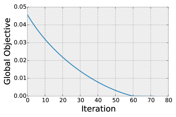
Figure 1: Synthetic global loss versus iteration. Our solution converges to the global optimum of zero.

5.2 Sentiment analysis task

With our optimization solution verified on the synthetic example, with known densities, we now seek to evaluate our performance on a real-world task with estimated densities. There are few readily available datasets for studying multiple source adaptation and even fewer for adaptation with regression tasks. We use the sentiment analysis dataset proposed by Blitzer et al. (2007) and used for multiple-source adaptation by Mansour et al. (2008, 2009). This dataset consists of product review text and rating labels taken from four domains: books (B), dvd (D), electronics (E), and kitchen (K), with $2000$ samples for each domain. We create 10 random splits of our data into a training set ($1600$ points) and test set ($400$ points) per domain.

Predictors: We defined a vocabulary of $2\mathord{,}500$ words that occur at least twice at the intersection of the four domains. These words were used to define feature vectors, where every sample point is encoded by the number of occurrences of each word. We trained our base hypotheses using support vector regression (SVR) with same hyper-parameters as in (Mansour et al., 2008, 2009).

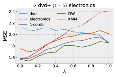
(a)

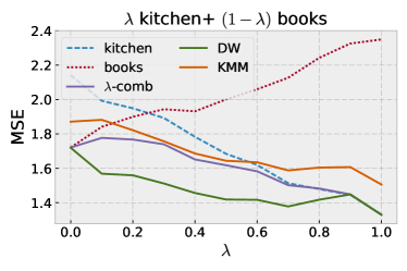
(b)

Figure 2: MSE sentiment analysis under mixture of two domains: (left) dvd and electronics or (right) kitchen and books.

Density estimation: In practice, the probability distributions ${\mathscr{D}}_{k}$ are not readily available to the learner. However, Theorem 5 extends the learning guarantees of our solution to the case where an estimate $\widehat{\mathscr{D}}_{k}$ is used in lieu of the ideal distribution ${\mathscr{D}}_{k}$, for each $k\in[p]$. Thus, here, we briefly discuss the problem of deriving an estimate $\widehat{\mathscr{D}}_{k}$ for each $k\in[p]$.

We used the same vocabulary defined for feature extraction to train a bigram statistical language model for each domain, using the OpenGrm library (Roark et al., 2012). Next, we randomly draw a sample set $S_{k}$ of $10\mathord{,}000$ sentences from each bigram language model. We define $\widehat{\mathscr{D}}_{k}$ to be the empirical distribution of $S_{k}$, which is a very close estimate of the marginal distribution of the language model, thus it is also a good estimate of ${\mathscr{D}}_{k}$. We approximate the label of a randomly generated sample $x_{i}$ by taking the average of the $h_{k}$s: $y_{i}=\sum_{\{k\colon x_{i}\in S_{k}\}}h_{k}(x_{i})/|\{k\colon x_{i}\in S_{k}\}|$. These randomly drawn samples were used to find the fixed-point $z$.

Note that we only use estimates of the marginal distributions (language models) to find $z$ and do not use any labels. We use the original product review text and rating labels for testing. Their densities $\widehat{\mathscr{D}}_{k}$ were estimated by the bigram language models directly, therefore a close estimate of ${\mathscr{D}}_{k}$.

Baselines: We compare against each source hypothesis, $h_{k}$, as well as the uniform combination of all hypotheses (unif), $\sum_{k=1}^{p}h_{k}/p$. We also compute a privileged baseline using the known $\lambda$ mixing parameter, $\lambda$-comb: $\sum_{k=1}^{p}\lambda_{k}h_{k}$. $\lambda$-comb is of course not accessible in practice since the target mixture $\lambda$ is not known to the user.

Note that our method (DW) produces a single predictor for any target distribution which is a mixture of source domains. For completeness, we compare against a previously proposed domain adaptation algorithm (Huang et al., 2006) known as KMM. However, it is important to note that the KMM model requires access to the unlabeled target data during adaptation and learns a new predictor per target domain. Thus KMM operates in a favorable learning setting when compared to our solution.

Given source data and unlabeled target data, KMM reweights samples from the source domain so that the mean input feature vector over the source domain is close to the mean input feature vector over target domain in reproducing kernel Hilbert space (RKHS). Then, it uses these sample weights on the source data to train a predictor using SVR. In our KMM experiments, we used the same kernel function as the one use for training the base hypotheses. We used the hyper-paramters $B=1000$ and $\epsilon=\frac{\sqrt{n}}{\sqrt{n}-1}$, where $n$ is number of training samples, as recommended by the authors (Huang et al., 2006). We denote by KMM the specifically trained predictor for each test data.

Prediction: We first considered the scenario where the target is a mixture of two source domains. For $\lambda$ varying from $0,0.1,0.2,\ldots,1$, the test set consists of $400\cdot\lambda$ points from the first domain and $400\cdot(1-\lambda)$ points from second domain. We used $1600$ training points for KMM ($800$ per domain), which coincides with the sample size used to learn each base hypothesis, and used $50\%$ of the test dataset for KMM adaptation. We report experimental results in Figures 2a and 2b. They show that our distribution weighted predictor DW outperforms all baseline predictors despite the privileged learning scenarios of $\lambda$-comb and KMM.

Next, we compared the performance of DW with the baseline predictors on various target mixtures, including each domain individually, the combination of any two and three domains, and all four domains. More mixture combinations are available in the supplementary material. We used again $1600$ training points ($400$ per domain) and $50\%$ testing data for KMM algorithm. Table 1 reports the mean and standard deviations of MSE over $10$ repetitions. Each column corresponds to a different target test data source. Our distribution weighted method DW outperforms all baseline predictors across all test domains. Observe that, even when the target is a single source domain, our method successfully outperforms the predictor which is trained and tested on the same domain. Notice that this can happen even when each $h_{k}$ is the best predictor in some hypothesis set $H_{k}$ for its own domain, since our distribution weighted predictor DW belongs to a more complex family of hypotheses.

Overall, these results show that our single DW predictor has strong performance across various test domains, confirming the robustness suggested by our theory.

6 Conclusion

We presented an algorithm for multiple-source domain adaptation in the common scenario where the squared loss is used. Our algorithm computes a distribution-weighted combination of predictors for each source domain which we showed to admit very favorable guarantees. We further demonstrated the effectiveness of our algorithm empirically in experiments with both artificial data sets and a sentiment analysis task.

In this appendix, we give detailed proofs of several of theorems for multiple-source adaptation for regression (Section A. We present an analysis of the stationary points for our min-max optimization problem in Section B. Finally, in Section C, we report the results of several additional experiments demonstrating the benefits of our robust solutions.

Appendix A Proofs

Theorem 3.

For any $\delta>0$, there exists $\eta>0$ and $z\in\Delta$, such that $\mathcal{L}({\mathscr{D}}_{\lambda},h_{z}^{\eta})\leq\epsilon+\delta$  for any mixture parameter $\lambda\in\Delta$.

Proof.

We first upper bound, for an arbitrary $z\in\Delta$, the expected loss of $h_{z}^{\eta}$ with respect to the mixture distribution ${\mathscr{D}}_{z}$ defined using the same $z$, that is $\mathcal{L}({\mathscr{D}}_{z},h_{z}^{\eta})=\sum_{k=1}^{p}z_{k}\mathcal{L}({\mathscr{D}}_{k},h_{z}^{\eta})$. By definition of $h_{z}^{\eta}$ and ${\mathscr{D}}_{z}$, we can write

$$\mathcal{L}({\mathscr{D}}_{z},h_{z}^{\eta})$$

$$=\sum_{(x,y)}{\mathscr{D}}_{z}(x,y)L(h_{z}^{\eta}(x),y)$$

$$=\sum_{(x,y)}{\mathscr{D}}_{z}(x,y)L\mspace{-2.0mu}\left(\mspace{-1.0mu}\sum_{k=1}^{p}\frac{z_{k}{\mathscr{D}}^{1}_{k}(x)+\eta\frac{{\mathscr{U}}^{1}(x)}{p}}{{\mathscr{D}}^{1}_{z}(x)+\eta{\mathscr{U}}^{1}(x)}h_{k}(x),y\right)\mspace{-4.0mu}.$$

By convexity of $L$, this implies that

$$\mathcal{L}({\mathscr{D}}_{z},h_{z}^{\eta})$$

$$\leq\sum_{(x,y)}{\mathscr{D}}_{z}(x,y)\sum_{k=1}^{p}\frac{z_{k}{\mathscr{D}}^{1}_{k}(x)+\eta\frac{{\mathscr{U}}^{1}(x)}{p}}{{\mathscr{D}}^{1}_{z}(x)+\eta{\mathscr{U}}^{1}(x)}L\big{(}h_{k}(x),y\big{)}$$

$$\leq\sum_{(x,y)}{\mathscr{D}}_{z}(y|x){\mathscr{D}}^{1}_{z}(x)\sum_{k=1}^{p}\frac{z_{k}{\mathscr{D}}^{1}_{k}(x)+\eta\frac{{\mathscr{U}}^{1}(x)}{p}}{{\mathscr{D}}^{1}_{z}(x)+\eta{\mathscr{U}}^{1}(x)}L\big{(}h_{k}(x),y\big{)}$$

$$\leq\sum_{(x,y)}{\mathscr{D}}_{z}(y|x)\sum_{k=1}^{p}\bigg{(}z_{k}{\mathscr{D}}^{1}_{k}(x)+\eta\frac{{\mathscr{U}}^{1}(x)}{p}\bigg{)}L\big{(}h_{k}(x),y\big{)}.$$

Next, observe that ${\mathscr{D}}_{z}(y|x)=\sum_{k=1}^{p}\frac{z_{k}{\mathscr{D}}^{1}_{k}(x)}{{\mathscr{D}}^{1}_{z}(x)}{\mathscr{D}}_{k}(y|x)={\mathscr{D}}_{k}(y|x)$ for any $k\in[1,p]$ since by assumption ${\mathscr{D}}_{k}(y|x)$ does not depend on $k$. Thus,

$$\mathcal{L}({\mathscr{D}}_{z},h_{z}^{\eta})$$

$$\leq\sum_{(x,y)}{\mathscr{D}}_{z}(y|x)\sum_{k=1}^{p}\bigg{(}z_{k}{\mathscr{D}}^{1}_{k}(x)+\eta\frac{{\mathscr{U}}^{1}(x)}{p}\bigg{)}L\big{(}h_{k}(x),y\big{)}$$

$$=\sum_{(x,y)}\mspace{-2.0mu}\sum_{k=1}^{p}\bigg{(}\mspace{-2.0mu}z_{k}{\mathscr{D}}_{k}(y|x){\mathscr{D}}^{1}_{k}(x)+\eta{\mathscr{D}}_{k}(y|x)\frac{{\mathscr{U}}^{1}(x)}{p}\mspace{-2.0mu}\bigg{)}\mspace{-2.0mu}L\big{(}h_{k}(x),y\big{)}$$

$$=\sum_{k=1}^{p}z_{k}\mathcal{L}({\mathscr{D}}_{k},h_{k})+\frac{\eta}{p}\sum_{k=1}^{p}\sum_{(x,y)}{\mathscr{D}}_{k}(y|x){\mathscr{U}}^{1}(x)L\big{(}h_{k}(x),y\big{)}$$

$$\leq\sum_{k=1}^{p}z_{k}\mathcal{L}({\mathscr{D}}_{k},h_{k})+\eta M$$

$$\leq\sum_{k=1}^{p}z_{k}\epsilon+\eta M=\epsilon+\eta M.$$

Now, choose $z\in\Delta$ as in the statement of Lemma 2. Then, the following holds for any mixture distribution ${\mathscr{D}}_{\lambda}$:

$$\mathcal{L}({\mathscr{D}}_{\lambda},h_{z}^{\eta}) =\sum_{k=1}^{p}\lambda_{k}\mathcal{L}({\mathscr{D}}_{k},h_{z}^{\eta})$$

$$\leq\sum_{k=1}^{p}\lambda_{k}\big{(}\mathcal{L}({\mathscr{D}}_{z},h_{z}^{\eta})+\eta^{\prime}\big{)}$$

$$=\mathcal{L}({\mathscr{D}}_{z},h_{z}^{\eta})+\eta^{\prime}\leq\epsilon+\eta M+\eta^{\prime}.$$

Setting $\eta=\frac{\delta}{2M}$ and $\eta^{\prime}=\frac{\delta}{2}$ concludes the proof. ∎

Theorem 4.

Let ${\mathscr{D}}_{T}$ be an arbitrary target distribution. For any $\delta>0$, there exists $\eta>0$ and $z\in\Delta$, such that the following inequality holds for any $\alpha>1$:

$$\mathcal{L}({\mathscr{D}}_{T},h_{z}^{\eta})\leq\Big{[}(\epsilon+\delta)\,{\mathsf{d}}_{\alpha}({\mathscr{D}}_{T}\parallel\mathcal{D})\Big{]}^{\frac{\alpha-1}{\alpha}}M^{\frac{1}{\alpha}}.$$

Proof.

For any hypothesis $h\colon\mathcal{X}\to\mathcal{Y}$ and any distribution ${\mathscr{D}}$, by Hölder’s inequality, the following holds:

$$\mathcal{L} ({\mathscr{D}}_{T},h)=\sum_{(x,y)\in\mathcal{X}\times\mathcal{Y}}{\mathscr{D}}_{T}(x,y)L(h(x),y)$$

$$=\sum_{(x,y)\in\mathcal{X}\times\mathcal{Y}}\left[\frac{{\mathscr{D}}_{T}(x,y)}{{\mathscr{D}}(x,y)^{\frac{\alpha-1}{\alpha}}}\right]\left[{\mathscr{D}}(x,y)^{\frac{\alpha-1}{\alpha}}L(h(x),y)\right]$$

$$\leq\left[\sum_{(x,y)}\frac{{\mathscr{D}}_{T}(x,y)^{\alpha}}{{\mathscr{D}}(x,y)^{\alpha-1}}\right]^{\frac{1}{\alpha}}\left[\sum_{(x,y)}{\mathscr{D}}(x,y)L(h(x),y)^{\frac{\alpha}{\alpha-1}}\right]^{\mspace{-8.0mu}\frac{\alpha-1}{\alpha}}\mspace{-25.0mu}.$$

Thus, by definition of ${\mathsf{d}}_{\alpha}$, for any $h$ such that $L(h(x),y)\leq M$ for all $(x,y)$, we can write

$$\mathcal{L}({\mathscr{D}}_{T},h)$$

$$\leq{\mathsf{d}}_{\alpha}({\mathscr{D}}_{T}\parallel{\mathscr{D}})^{\frac{\alpha-1}{\alpha}}\mspace{-8.0mu}\left[\sum_{(x,y)}{\mathscr{D}}(x,y)L(h(x),y)^{\frac{\alpha}{\alpha-1}}\mspace{-4.0mu}\right]^{\mspace{-8.0mu}\frac{\alpha-1}{\alpha}}$$

$$={\mathsf{d}}_{\alpha}({\mathscr{D}}_{T}\parallel{\mathscr{D}})^{\frac{\alpha-1}{\alpha}}\mspace{-8.0mu}\left[\sum_{(x,y)}{\mathscr{D}}(x,y)L(h(x),y)L(h(x),y)^{\frac{1}{\alpha-1}}\mspace{-4.0mu}\right]^{\mspace{-8.0mu}\frac{\alpha-1}{\alpha}}$$

$$\leq{\mathsf{d}}_{\alpha}({\mathscr{D}}_{T}\parallel{\mathscr{D}})^{\frac{\alpha-1}{\alpha}}\left[\sum_{(x,y)}{\mathscr{D}}(x,y)L(h(x),y)M^{\frac{1}{\alpha-1}}\right]^{\mspace{-8.0mu}\frac{\alpha-1}{\alpha}}$$

$$\leq\Big{[}{\mathsf{d}}_{\alpha}({\mathscr{D}}_{T}\parallel{\mathscr{D}})\,\mathcal{L}({\mathscr{D}},h)\Big{]}^{\mspace{-6.0mu}\frac{\alpha-1}{\alpha}}M^{\frac{1}{\alpha}}.$$

Now, by Theorem 3, there exists $z\in\Delta$ and $\eta>0$ such that $\mathcal{L}({\mathscr{D}},h_{z}^{\eta})\leq\epsilon+\delta$ for any mixture distribution ${\mathscr{D}}\in\mathcal{D}$. Thus, in view of the previous inequality, we can write,for any ${\mathscr{D}}\in\mathcal{D}$,

$$\mathcal{L}({\mathscr{D}}_{T},h_{z}^{\eta})\leq\Big{[}(\epsilon+\delta)\,{\mathsf{d}}_{\alpha}({\mathscr{D}}_{T}\parallel{\mathscr{D}})\Big{]}^{\frac{\alpha-1}{\alpha}}M^{\frac{1}{\alpha}}.$$

Taking the infimum of the right-hand side over all ${\mathscr{D}}\in\mathcal{D}$ completes the proof. ∎

Theorem 5.

Let ${\mathscr{D}}_{T}$ be an arbitrary target distribution. Then, for any $\delta>0$, there exists $\eta>0$ and $z\in\Delta$, such that the following inequality holds for any $\alpha>1$:

$$\mathcal{L}({\mathscr{D}}_{T},\widehat{h}_{z}^{\eta})\leq\Big{[}(\widehat{\epsilon}+\delta)\,{\mathsf{d}}_{\alpha}({\mathscr{D}}_{T}\parallel\widehat{\mathcal{D}})\Big{]}^{\frac{\alpha-1}{\alpha}}M^{\frac{1}{\alpha}}.$$

Proof.

By the first part of the proof of Theorem 4, for any $k\in[p]$ and $\alpha>1$, the following inequality holds:

$$\mathcal{L}(\widehat{\mathscr{D}}_{k},h_{k}) \leq\Big{[}{\mathsf{d}}_{\alpha}(\widehat{\mathscr{D}}_{k}\parallel{\mathscr{D}}_{k})\,\mathcal{L}({\mathscr{D}}_{k},h_{k})\Big{]}^{\frac{\alpha-1}{\alpha}}M^{\frac{1}{\alpha}}$$

$$\leq\Big{[}\epsilon\,{\mathsf{d}}_{\alpha}(\widehat{\mathscr{D}}_{k}\parallel{\mathscr{D}}_{k})\Big{]}^{\frac{\alpha-1}{\alpha}}M^{\frac{1}{\alpha}}\leq\widehat{\epsilon}.$$

We can now apply the result of Theorem 4 (with $\widehat{\epsilon}$ instead of $\epsilon$ and $\widehat{\mathscr{D}}_{k}$ instead of ${\mathscr{D}}_{k}$). In view that, there exists $\eta>0$ and $z\in\Delta$ such that

$$\mathcal{L}({\mathscr{D}}_{T},h_{z}^{\eta})\leq\Big{[}(\widehat{\epsilon}+\delta)\,{\mathsf{d}}_{\alpha}({\mathscr{D}}_{T}\parallel\widehat{\mathscr{D}})\Big{]}^{\frac{\alpha-1}{\alpha}}M^{\frac{1}{\alpha}},$$

for any distribution $\widehat{\mathscr{D}}$ in the family $\widehat{\mathcal{D}}$. Taking the infimum over all $\widehat{\mathscr{D}}$ in $\widehat{\mathcal{D}}$ completes the proof. ∎

Appendix B Stationary Point Analysis

In this section we explicitly analyze the stationary point conditions for the min-max optimization problem:

$$\min_{z} \ f(z)$$

s.t. $$\ g_{k}(z)\leq 0,\forall k\in[p],\ h(z)=0,$$

where

$$f(z) =\max_{k\in[p]}\mathcal{L}({\mathscr{D}}_{k},h_{z}^{\eta})-\mathcal{L}({\mathscr{D}}_{z},h_{z}^{\eta}),$$

$$g_{k}(z) =-z_{k},\ h(z)=\sum_{k=1}^{p}z_{k}-1.$$

For simplicity, we assume ${\mathscr{D}}_{k}(x)>0,\forall k\in[p],\forall x\in\mathcal{X}$, and let $\eta=0$. D.C. algorithm converges to a stationary point $z^{*}\in\Delta$. Under suitable constraint qualification, there exists KKT multipliers $\alpha_{k},k\in[p]$ and $\beta$ such that

$$-\left[\sum_{k=1}^{p}\alpha_{k}\nabla g_{k}\left(z^{*}\right)+\beta\nabla_{z}h\left(z^{*}\right)\right] \in\partial_{z}f(z^{*})$$ (14)

$$\alpha_{k}g_{k}(z^{*})=0,\ \alpha_{k} \geq 0,\ k\in[p]$$

where the set of sub-gradients of $f(z)$ is subset of a convex hull:

$$\partial_{z}f(z)\subseteq\text{Co}\left\{\nabla_{z}\mathcal{L}({\mathscr{D}}_{k},h_{z})-\nabla_{z}\mathcal{L}({\mathscr{D}}_{z},h_{z}),k\in[p]\right\}.$$

Observer that, for any fixed $x\in\mathcal{X}$ and $z\in\mathbb{R}^{p}$ , $z^{T}\nabla_{z}h_{z}(x)=0$. It follows that $z^{T}\nabla_{z}\mathcal{L}({\mathscr{D}}_{k},h_{z})=0,\ \forall k\in[p]$. Thus, by taking inner product of $z^{*}$ and elements in $\partial_{z}f(z^{*})$, we obtain

$$z^{*T}\partial_{z}f(z^{*})=-z^{*T}\nabla_{z}\mathcal{L}({\mathscr{D}}_{z^{*}},h_{z^{*}})=-\mathcal{L}({\mathscr{D}}_{z^{*}},h_{z^{*}}).$$

On the other hand,

$$z^{*T}\left[\sum_{k=1}^{p}\alpha_{k}\nabla g_{k}(z^{*})+\beta\nabla_{z}h(z^{*})\right]=-\sum_{k}\alpha_{k}z_{k}^{*}+\beta=\beta.$$

Therefore $\beta=\mathcal{L}({\mathscr{D}}_{z^{*}},h_{z^{*}})$, thus we obtain the following simplified stationary point conditions: there exits $\alpha_{k},k\in[p]$ such that

$$\left[\mathcal{L}({\mathscr{D}}_{z^{*}},h_{z^{*}})-\alpha_{1},\ldots,\mathcal{L}({\mathscr{D}}_{z^{*}},h_{z^{*}})-\alpha_{p}\right]^{T} \in-\partial_{z}f\left(z^{*}\right)$$

$$\alpha_{k}z_{k}^{*}=0,\ \alpha_{k} \geq 0,\ k\in[p].$$

Appendix C More Experiment Results

In this section we provide more experiment results to show that our distribution weighted predictor DW is robust across various test data mixtures.

	Test Data
	KB	KE	DB	DE
K	1.87$\pm$0.08	1.57$\pm$0.06	2.25$\pm$0.08	1.94$\pm$0.10
D	2.12$\pm$0.07	2.11$\pm$0.05	1.95$\pm$0.06	1.94$\pm$0.06
B	1.96$\pm$0.07	2.21$\pm$0.06	1.87$\pm$0.07	2.13$\pm$0.05
E	2.05$\pm$0.05	1.60$\pm$0.05	2.36$\pm$0.07	1.91$\pm$0.07
unif	1.74$\pm$0.05	1.62$\pm$0.04	1.85$\pm$0.05	1.73$\pm$0.06
KMM	1.78$\pm$0.12	1.65$\pm$0.10	1.97$\pm$0.13	1.88$\pm$0.08
DW	1.59$\pm$0.05	1.47$\pm$0.04	1.75$\pm$0.05	1.64$\pm$0.05

Table 2: MSE on the sentiment analysis dataset. Using the learned $z$, our distribution weighted method DW outperforms all competing baselines in terms of robustness across test domains. We compare against source only baselines for each domain, K, D, B, E, a uniform weighted predictor unif, and KMM.

	Test Data
	KDBE	KDBE	KDBE	KDBE	KDBE	KDBE	KDBE	KDBE	KDBE	KDBE
K	1.78$\pm$0.05	1.94$\pm$0.10	1.96$\pm$0.08	1.84$\pm$0.07	1.86$\pm$0.10	1.87$\pm$0.07	1.79$\pm$0.08	1.96$\pm$0.10	1.89$\pm$0.10	1.89$\pm$0.08
D	2.02$\pm$0.10	1.98$\pm$0.10	2.06$\pm$0.11	2.05$\pm$0.09	2.01$\pm$0.13	2.05$\pm$0.12	2.04$\pm$0.12	2.03$\pm$0.12	2.02$\pm$0.13	2.06$\pm$0.12
B	2.01$\pm$0.12	2.01$\pm$0.14	1.94$\pm$0.14	2.06$\pm$0.11	2.01$\pm$0.15	1.98$\pm$0.14	2.05$\pm$0.13	1.98$\pm$0.15	2.04$\pm$0.14	2.01$\pm$0.13
E	1.93$\pm$0.08	2.04$\pm$0.10	2.08$\pm$0.10	1.89$\pm$0.08	2.00$\pm$0.10	2.01$\pm$0.09	1.91$\pm$0.08	2.08$\pm$0.10	1.97$\pm$0.08	1.99$\pm$0.08
unif	1.69$\pm$0.06	1.74$\pm$0.07	1.75$\pm$0.08	1.70$\pm$0.06	1.72$\pm$0.09	1.72$\pm$0.08	1.69$\pm$0.07	1.75$\pm$0.08	1.72$\pm$0.08	1.73$\pm$0.08
KMM	1.83$\pm$0.12	1.92$\pm$0.14	1.87$\pm$0.15	1.85$\pm$0.13	1.85$\pm$0.16	1.86$\pm$0.14	1.85$\pm$0.15	1.90$\pm$0.14	1.89$\pm$0.16	1.90$\pm$0.14
DW	1.55$\pm$0.08	1.62$\pm$0.08	1.59$\pm$0.09	1.56$\pm$0.08	1.58$\pm$0.10	1.57$\pm$0.10	1.55$\pm$0.09	1.61$\pm$0.10	1.59$\pm$0.08	1.58$\pm$0.09

Table 3: MSE on the sentiment analysis dataset. Using the learned $z$, our distribution weighted method DW outperforms all competing baselines in terms of robustness across test domains. We compare against source only baselines for each domain, K, D, B, E, a uniform weighted predictor unif, and KMM.

Table 2 shows MSE on various combinations of two domains that is not included in Table 1.

Table 3 reports MSE on additionally test domain mixtures. The first four target mixtures correspond to various orderings of $\{0.4,0.2,0.2,0.2\}$. The next six target mixtures correspond to various orderings of $\{0.3,0.3,0.2,0.2\}$. In column title we bold the domain(s) with highest weight.

References

• Arndt [2004] C. Arndt. Information Measures: Information and its Description in Science and Engineering. Signals and Communication Technology. Springer Verlag, 2004.
• Blitzer et al. [2007] J. Blitzer, M. Dredze, and F. Pereira. Biographies, bollywood, boom-boxes and blenders: Domain adaptation for sentiment classification. In Association for Computational Linguistics (ACL), 2007.
• Chattopadhyay et al. [2012] R. Chattopadhyay, Q. Sun, W. Fan, I. Davidson, S. Panchanathan, and J. Ye. Multisource domain adaptation and its application to early detection of fatigue. ACM Transactions on Knowledge Discovery from Data (TKDD), 6(4):18, 2012.
• Chen and Deng [2008] X. Chen and X. Deng. Matching algorithmic bounds for finding a brouwer fixed point. J. ACM, 55(3), 2008.
• Dredze et al. [2008] M. Dredze, K. Crammer, and F. Pereira. Confidence-weighted linear classification. In International Conference on Machine Learning (ICML), 2008.
• Duan et al. [2012a] L. Duan, D. Xu, and S.-F. Chang. Exploiting web images for event recognition in consumer videos: A multiple source domain adaptation approach. In Computer Vision and Pattern Recognition (CVPR), 2012 IEEE Conference on, pages 1338–1345. IEEE, 2012a.
• Duan et al. [2012b] L. Duan, D. Xu, and I. W.-H. Tsang. Domain adaptation from multiple sources: A domain-dependent regularization approach. IEEE Transactions on Neural Networks and Learning Systems, 23(3):504–518, 2012b.
• Eaves [1972] B. C. Eaves. Matching algorithmic bounds for finding a brouwer fixed point. Math. Progr., 3:1–22, 1972.
• Ganin and Lempitsky [2015] Y. Ganin and V. Lempitsky. Unsupervised domain adaptation by backpropagation. In International Conference in Machine Learning (ICML), 2015.
• Girshick et al. [2014] R. Girshick, J. Donahue, T. Darrell, and J. Malik. Rich feature hierarchies for accurate object detection and semantic segmentation. In In Proc. CVPR, 2014.
• Gong et al. [2012] B. Gong, Y. Shi, F. Sha, and K. Grauman. Geodesic flow kernel for unsupervised domain adaptation. In Proc. CVPR, 2012.
• Gong et al. [2013a] B. Gong, K. Grauman, and F. Sha. Connecting the dots with landmarks: Discriminatively learning domain-invariant features for unsupervised domain adaptation. In ICCV, 2013a.
• Gong et al. [2013b] B. Gong, K. Grauman, and F. Sha. Reshaping visual datasets for domain adaptation. In NIPS, 2013b.
• Hirsch et al. [1989] M. D. Hirsch, C. H. Papadimitriou, and S. A. Vavasis. Exponential lower bounds for finding brouwer fix points. J. Complexity, 5(4):379–416, 1989.
• Hoffman et al. [2012] J. Hoffman, B. Kulis, T. Darrell, and K. Saenko. Discovering latent domains for multisource domain adaptation. In European Conference on Computer Vision (ECCV), 2012.
• Hoffman et al. [2013] J. Hoffman, E. Rodner, J. Donahue, K. Saenko, and T. Darrell. Efficient learning of domain-invariant image representations. In International Conference on Learning Representations, 2013.
• Horst and Thoai [1999] R. Horst and N. V. Thoai. DC programming: overview. Journal of Optimization Theory and Applications, 103(1):1–43, 1999.
• Huang et al. [2006] J. Huang, A. J. Smola, A. Gretton, K. M. Borgwardt, and B. Schölkopf. Correcting sample selection bias by unlabeled data. In Advances in Neural Information Processing Systems (NIPS), volume 19, pages 601–608, 2006.
• Kuhn [1968] H. Kuhn. Simplicial approximations of fixed points. Proceedings of the National Academy of Sciences, 61:1238–1242, 1968.
• Liao [2013] H. Liao. Speaker adaptation of context dependent deep neural networks. In ICASSP, 2013.
• Long et al. [2015] M. Long, Y. Cao, J. Wang, and M. I. Jordan. Learning transferable features with deep adaptation networks. In International Conference in Machine Learning (ICML), 2015.
• Mansour et al. [2008] Y. Mansour, M. Mohri, and A. Rostamizadeh. Domain adaptation with multiple sources. In NIPS, 2008.
• Mansour et al. [2009] Y. Mansour, M. Mohri, and A. Rostamizadeh. Multiple source adaptation and the Rényi divergence. In UAI, pages 367–374, 2009.
• Merrill [1972] O. H. Merrill. Applications and Extensions of an Algorithm That Computes Fixed Points of Certain Upper Semi-continuous Point to Set Mappings. PhD thesis, Dept. of Industrial Engineering, University of Michigan, 1972.
• Muandet et al. [2013] K. Muandet, D. Balduzzi, and B. Schölkopf. Domain generalization via invariant feature representation. In Proceedings of ICML, pages 10–18, 2013.
• Pan and Yang [2010] S. J. Pan and Q. Yang. A survey on transfer learning. In IEEE Transactions on Knowledge and Data Engineering, 2010.
• Rényi [1961] A. Rényi. On measures of entropy and information. In Proceedings of the Fourth Berkeley Symposium on Mathematical Statistics and Probability, volume 1, pages 547–561, 1961.
• Roark et al. [2012] B. Roark, R. Sproat, C. Allauzen, M. Riley, J. Sorensen, and T. Tai. The opengrm open-source finite-state grammar software libraries. In Proceedings of the ACL 2012 System Demonstrations, pages 61–66. Association for Computational Linguistics, 2012.
• Saenko et al. [2010] K. Saenko, B. Kulis, M. Fritz, and T. Darrell. Adapting visual category models to new domains. In Proc. ECCV, 2010.
• Scarf [1967] H. Scarf. The approximation of fixed points of a continuous mapping. SIAM J. Appl. Math, 15(5), 1967.
• Schweikert et al. [2009] G. Schweikert, G. Rätsch, C. Widmer, and B. Schölkopf. An empirical analysis of domain adaptation algorithms for genomic sequence analysis. In Advances in Neural Information Processing Systems, pages 1433–1440, 2009.
• Sriperumbudur and Lanckriet [2012] B. K. Sriperumbudur and G. R. G. Lanckriet. A proof of convergence of the concave-convex procedure using Zangwill’s theory. Neural Computation, 24(6):1391–1407, 2012.
• Tao and An [1997] P. D. Tao and L. T. H. An. Convex analysis approach to DC programming: theory, algorithms and applications. Acta Mathematica Vietnamica, 22(1):289–355, 1997.
• Tao and An [1998] P. D. Tao and L. T. H. An. A DC optimization algorithm for solving the trust-region subproblem. SIAM Journal on Optimization, 8(2):476–505, 1998.
• Torralba and Efros [2011] A. Torralba and A. Efros. Unbiased look at dataset bias. In CVPR, 2011.
• Tzeng et al. [2015] E. Tzeng, J. Hoffman, T. Darrell, and K. Saenko. Simultaneous deep transfer across domains and tasks. In International Conference in Computer Vision (ICCV), 2015.
• Xu et al. [2014] Z. Xu, W. Li, L. Niu, and D. Xu. Exploiting low-rank structure from latent domains for domain generalization. In European Conference in Computer Vision (ECCV), 2014.
• Yang et al. [2007] J. Yang, R. Yan, and A. G. Hauptmann. Cross-domain video concept detection using adaptive svms. ACM Multimedia, 2007.
• Yuille and Rangarajan [2003] A. L. Yuille and A. Rangarajan. The concave-convex procedure. Neural Computation, 15(4):915–936, 2003.