Autoresonant excitation of Bose-Einstein condensates

Abstract

Controlling the state of a Bose-Einstein condensate driven by a chirped frequency perturbation in a one-dimensional anharmonic trapping potential is discussed. By identifying four characteristic time scales in this chirped-driven problem, three dimensionless parameters $P_{1,2,3}$ are defined describing the driving strength, the anharmonicity of the trapping potential, and the strength of the particles interaction, respectively. As the driving frequency passes the linear resonance in the problem, and depending on the location in the $P_{1,2,3}$ parameter space, the system may exhibit two very different evolutions, i.e. the quantum energy ladder climbing (LC) and the classical autoresonance (AR). These regimes are analysed both in theory and simulations with the emphasis on the effect of the interaction parameter $P_{3}$. In particular, the transition thresholds on the driving parameter $P_{1}$ and their width in $P_{1}$ in both the AR and LC regimes are discussed. Different driving protocols are also illustrated, showing efficient control of excitation and de-excitation of the condensate.

I Introduction

Unique properties of Bose-Einstein condensates (BEC) attracted enormous interest in the last decades as a very flexible framework for experimental and theoretical research in many-body physics and a promising basis for new technologies. Modern applications require understanding of nonlinear dynamics of the condensates. Nonlinear dynamics is especially interesting in anharmonic trapping potentials, when motion of the center of mass is coupled to internal degrees of freedom Dobson_1994 , and may even become chaotic Ott_2003 . In this paper we take advantage of the anharmonic potential to excite a quasi-one-dimensional condensate from the ground state to a high energy level. The basic idea is to use a driving perturbation with a slowly varying frequency to transfer the population from the ground quantum state to the first excited state, then to the second, and so on. This dynamical process, when only two energy eigenstates are resonantly coupled at a time, is the ladder climbing (LC) regime.

The classical counterpart of the ladder climbing is the autoresonance (AR), the phenomenon discovered by Veksler and McMillan in 1944 Veksler_1944 and referred to as the phase stability principle at the time. Nowadays, the AR has multitude of applications in such diverse areas as hydrodynamics Friedland_1999 ; Friedland_2002 ; Assaf_2005 , plasmas Fajans_1999 ; Lindberg_2006 ; Yaakobi_2008 , magnetism Kalyakin_2007 ; Batalov_2013 ; Klughertz_2015 , nonlinear optics Barak_2009 , molecular physics Marcus_2004 , planetary dynamics Friedland_2001 etc. The AR in BECs was previously studied in Nicolin_2007 for the case of oscillating scattering length. The excitation of a BEC from the ground state to the first energy eigenstate using optimal control was investigated experimentally in Ref. Bucker_2013 .

In this paper we consider Gross-Pitaevskii model GP

$$i\hbar\Psi_{t} +\frac{\hbar^{2}}{2m}\Psi_{xx}-\left(U+g|\Psi|^{2}\right)\Psi=0,$$ (1)

$$U(x,t) =m\omega_{0}^{2}\left(\frac{x^{2}}{2}-\beta\frac{x^{4}}{4}\right)+\varepsilon x\cos\varphi(t),$$ (2)

which describes a BEC in a trap with the anharmonic potential $U(x,t)$ perturbed by a small amplitude oscillating drive. Here $\beta>0$ is the anharmonicity parameter assumed to be small. The frequency of the drive $\omega(t)=\dot{\varphi}(t)=\omega_{0}-\alpha t$ slowly decreases in time ($\alpha>0$) and passes through the linear resonance frequency $\omega_{0}$ in the problem at $t=0$. We assume that the wave function is normalized to unity and, thus, parameter $g$ is proportional to the total number of particles in the condensate. Both the classical AR and the quantum LC in the linear limit ($g=0$) of Eq. (1), i.e., the quantum Duffing oscillator, were studied in Refs. Marcus_2004 ; Barth_2011 ; Andresen_2011 ; Shalibo_2012 .

In this work, we focus on the nonlinear effects due to the interaction of the particles in the condensate. As a first step, we adopt the notations used in Ref. Barth_2011 to allow comparison with the linear case. To this end, we classify different dynamical regimes of Eq. (1) in terms of parameters $P_{1}$, $P_{2}$ used in Ref. Barth_2011 and introduce a new parameter $P_{3}$, characterizing the nonlinearity in the problem. These parameters are constructed using four characteristic time scales in the problem: the inverse Rabi frequency $T_{R}=\sqrt{2m\hbar\omega_{0}}/\varepsilon$, the frequency sweep time scale $T_{S}=\alpha^{-1/2}$, the anharmonic time scale $T_{A}=3\hbar\beta/(4m\alpha)$ of the trapping potential, and the nonlinear time scale $T_{N}=g/(\hbar\alpha\ell)$, where $\ell=\sqrt{{\hbar}/{m\omega_{0}}}$ is the characteristic width of the harmonic oscillator. Time $T_{A}$ is the time of passage of the frequency $\omega(t)$ through the anharmonic frequency shift between the first two levels of the energy ladder. Similarly, $T_{N}$ is the time of passage through the nonlinear frequency shift. Then, our three dimensionless parameters are defined as

$$\begin{split}P_{1}=\frac{T_{S}}{T_{R}}=\frac{\varepsilon}{\sqrt{2m\hbar\omega_{0}\alpha}}&,\quad P_{2}=\frac{T_{A}}{T_{S}}=\frac{3\hbar\beta}{4m\sqrt{\alpha}},\\ P_{3}=\frac{T_{N}}{T_{S}}&=\frac{g}{\hbar\ell\sqrt{\alpha}}\end{split}$$ (3)

and characterize the strength of the drive, the anharmonicity of the trapping potential and the nonlinearity of the condensate, respectively. We limit our discussion to the case of the positive nonlinearity (repulsion), $P_{3}>0$. The scope of the paper is as follows. In Sec. II we study the dynamics of our system in the energy basis of the quantum harmonic oscillator and find a domain in $P_{1,2,3}$ parameter space where the successive quantum energy ladder climbing process takes place. In Sec. III, we discuss the opposite limit of semiclassical dynamics. The details of our numerical simulations are presented in Sec. IV and the conclusions are summarized in Sec. V.

II Quantum LC regime

Here we focus on the LC regime, where the quantum nature of the system is mostly pronounced. In this case, it is convenient to express Eq. (1) in the energy basis of the linear harmonic oscillator $\Psi(x,t)=\sum_{n}c_{n}(t)\psi_{n}(x)$, yielding

$$\begin{split}i\hbar\frac{dc_{n}}{dt}&=E_{n}c_{n}+\frac{\varepsilon\ell}{\sqrt{2}}\left(\sqrt{n+1}\,c_{n+1}+\sqrt{n}\,c_{n-1}\right)\cos\varphi\\ &+g\sum_{klm}c_{k}c_{l}c_{m}^{\ast}\int_{-\infty}^{\infty}\psi_{n}\psi_{k}\psi_{l}\psi_{m}dx,\end{split}$$ (4)

where the approximate energy levels up to linear terms in $\beta$ are given by Landau1977quantum

$$E_{n}\approx\hbar\omega_{0}\left[n+\frac{1}{2}-\frac{3\beta\hbar}{8m\omega_{0}}\left(n^{2}+n+\frac{1}{2}\right)\right].$$

Introducing new variables $B_{n}=c_{n}\,e^{i\left(\frac{E_{0}t}{\hbar}+n\varphi\right)}$, we rewrite Eq. (4)  in the form

$$i \hbar\frac{dB_{n}}{dt}=\left[n\hbar\alpha t-\frac{3\beta\hbar}{8m\omega_{0}}n(n+1)\right]B_{n}$$

$$+\frac{\varepsilon\ell}{2\sqrt{2}}\left(\sqrt{n+1}\,B_{n+1}e^{-i\varphi}+\sqrt{n}\,B_{n-1}e^{i\varphi}\right)\left(e^{-i\varphi}+e^{i\varphi}\right)$$

$$+g\sum_{klm}B_{k}B_{l}B_{m}^{\ast}e^{i(n+m-k-l)\varphi}\int_{-\infty}^{\infty}\psi_{n}\psi_{k}\psi_{l}\psi_{m}dx$$

We also define the dimensionless time $\tau=\sqrt{\alpha}\,t$, coordinate $\xi=x/\ell$, and basis functions $\chi_{n}(\xi)=\sqrt{\ell}\,\psi_{n}(x)$, and use the rotating wave approximation (preserve only stationary terms in the driving and nonlinear components in Eq. (II)) to get a dimensionless system

$$i\frac{dB_{n}}{d\tau} =\Gamma_{n}B_{n}+\frac{P_{1}}{2}\left(\sqrt{n+1}\,B_{n+1}+\sqrt{n}\,B_{n-1}\right)$$

$$+P_{3}\sum_{kl}B_{k}B_{l}B_{l+k-n}^{\ast}\int_{-\infty}^{\infty}\chi_{n}\chi_{{}_{k}}\chi_{{}_{l}}\chi_{l+k-n}d\xi,$$ (6)

where the frequencies $\Gamma_{n}$ are $\Gamma_{n}=n\tau-\frac{P_{2}}{2}\,n(n+1)$.

The resonant population transfer between levels $n-1$ and $n$ [the Landau-Zener (LZ) transition Landau_1932 ] takes place when their time-dependent characteristic frequencies are matched: $\Gamma_{n-1}(\tau_{n})\approx\Gamma_{n}(\tau_{n})$, i.e. in the vicinity of $\tau_{n}=nP_{2}$. In terms of Eq. (4) this corresponds to the resonance condition $E_{n}-E_{n-1}\approx\hbar\,\omega(\tau_{n})$. Note that the anharmonicity parameter determines the time interval between successive LZ transitions $\Delta\tau=\tau_{n}-\tau_{n-1}=P_{2}$. These transitions can be treated independently provided their duration is much shorter than $\Delta\tau$. As suggested in Barth_2011 for the linear case $(P_{3}=0)$, the well-separated LZ transitions are expected when

$$P_{2}\gg 1+P_{1},$$ (7)

where the right hand side is a typical duration of a LZ transition in both adiabatic (slow passage through resonance) and fast transition limits Vitanov_1996 . This inequality defines the domain of essentially quantum dynamics in the parameter space $P_{1,2}$, if $P_{3}=0$. Later in this Section, we discuss how relation (7) is modified in the case of the nonlinear LZ transitions ($P_{3}\neq 0$).

Neglecting all states in (6), but those with amplitudes $u=B_{n-1}$ and $v=B_{n}$, we obtain the nonlinear LZ-type equations describing the isolated transition between the two states:

$$\begin{split}i\frac{du}{d\tau}&=\Gamma_{n-1}\,u+P_{3}\left(|u|^{2}I_{n-1}+2|v|^{2}J_{n}\right)u+\frac{P_{1}\sqrt{n}}{2}v,\\ i\frac{dv}{d\tau}&=\Gamma_{n}\,v+P_{3}\left(|v|^{2}I_{n}+2|u|^{2}J_{n}\right)v+\frac{P_{1}\sqrt{n}}{2}u,\end{split}$$ (8)

where $J_{n}=\int|\chi_{n-1}|^{2}|\chi_{n}|^{2}d\xi$, $I_{n}=\int|\chi_{n}|^{4}d\xi$, The nonlinear LZ model attracted significant attention recently Liu_2002 ; Zhang_2008 ; Trimborn_2010 , especially in the context of BECs in optical lattices. Nonlinearity may change the dynamics of the system significantly compared to the linear case. One deviation from the linear case is the breakdown of adiabaticity due to the bifurcation of nonlinear stationary states Wu_2000 ; Zobay_2000 . In this paper we focus on another property of the nonlinear LZ model, namely, the AR.

Equations (8) can be simplified using the conservation of the total probability $K_{n}=|u|^{2}+|v|^{2}$. Introducing the fractional population imbalance $S=({|v|^{2}-|u|^{2}})/{K_{n}}$ and the phase mismatch $\delta=\arg\left({v/u}\right)$, we obtain a set of real equations

$$\begin{split}\frac{dS}{d\tau}&=-\mu_{n}\sqrt{1-S^{2}}\sin\delta,\\ \frac{d\delta}{d\tau}&=\frac{P_{3}K_{n}f_{n}}{2}S-(\tau-\tau_{\ast})+\frac{P_{1}\sqrt{n}\,S}{\sqrt{1-S^{2}}}\cos\delta,\end{split}$$ (9)

where $f_{n}=4J_{n}-I_{n-1}-I_{n}$ and $\tau_{\ast}=nP_{2}-P_{3}K_{n}(I_{n}-I_{n-1})/2$ . The AR in a similar system was studied in Barak_2009 . Its main characteristic is a continuing phase locking as the phase mismatch $\delta$ remains bounded due to a persistent self-adjustment of the nonlinear frequency of the driven system to slowly varying driving frequency, i.e., $P_{3}K_{n}f_{n}S/2\approx(\tau-\tau_{\ast})$. However, the slow passage through resonance does not guarantee the AR. Indeed, if one assumes that only state $u$ is populated initially, that is $S\rightarrow-1$, then the AR requires the driving parameter $P_{1\text{ }}$to exceed a certain threshold Barak_2009

$$P_{1}>P_{1,cr}=\frac{0.82}{\sqrt{nP_{3}f_{n}K_{n}}}.$$ (10)

This condition (10) shows that the AR is an essentially nonlinear phenomenon and disappears when $P_{3}\rightarrow 0$.

A typical dynamics of the nonlinear LZ model is illustrated in Fig. 1.

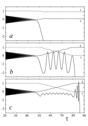
Figure 1: The phase mismatch $\delta$ (solid lines) and amplitudes (1 – $|u|^{2}$ and 2 – $|v|^{2}$, dashed lines) versus slow time $\tau$ in the nonlinear Landau-Zener transition for $P_{2}=50$, $P_{3}=300$. Panel (a) below the AR threshold $P_{1}=0.14<P_{1,cr}=0.15$, panel (b) just above the threshold $P_{1}=0.16$, and panel (c) well above the threshold $P_{1}=0.31$ when the AR phase-locking is observed; the parameters are $n=1$, $K_{1}=1$, and $f_{1}\approx 0.1$.

For a given nonlinearity $P_{3}$, the threshold condition (10) separates two different types of evolution of the system. If $P_{1}<P_{1,cr}$ (see Fig. 1$a$), the passage through the resonance at $\tau\approx\tau_{\ast}-P_{3}K_{n}f_{n}/2\approx 50$ yields a small excitation and a fast growth of the phase mismatch $\delta$ between the two states (see solid line in Fig. 1$a$). In contrast, we observe synchronization and nearly complete transition between the states when the coupling parameter exceeds the threshold, $P_{1}>P_{1,cr}$. Figures 1$b$ and 1$c$ illustrate this effect just beyond the threshold and far from the threshold, respectively. One can see that above the threshold the phase mismatch is bounded, exhibiting the phase-locking phenomenon characteristic of the AR. One can also see that the amplitudes vary significantly during the transition from $n-1$ to $n$ state. The phase-locking is destroyed only after the system almost completely transfers to the new state. As long as the phase-locking is sustained, the population imbalance increases on average as $S(\tau)\approx{2(\tau-\tau_{\ast})}/{P_{3}f_{n}K_{n}}$ with some superimposed modulations. In particular, $|u|^{2}\approx|v|^{2}$ at time $\tau\approx\tau_{\ast}\$($\tau_{\ast}=65$ in our examples). Since the maximal change of the population imbalance is $\Delta S=2$, the duration of the complete autoresonant transition can be estimated as

$$\tau_{AR}=P_{3}f_{n}K_{n}.$$

The most important characteristic of the LZ model is the transition probability $W_{n}={|v(\infty)|^{2}}/{K_{n}}$ for finding the system in the upper state if it was in the lower state initially. In the linear limit, this probability is given by the famous LZ formula

$$W_{n}=1-e^{-\frac{n\pi P_{1}^{2}}{2}}.$$ (11)

The numerical integration of the nonlinear LZ model (8) gives the transition probability shown in Fig. 2. The curve corresponding to $P_{3}=0$ coincides with the linear LZ result (11). The transition probability steepens as the nonlinearity $P_{3}$ increases and tends to a step-like function in the strongly nonlinear limit. The front of this step corresponds to the onset of the AR at $P_{1}\approx P_{1,cr}$. Once phase-locked, the system remains in this state until almost complete population inversion is achieved, as indicated by transition probability (the height of the step) close to unity in Fig. 2. This means that the threshold $\eqref{eq:P1cr}$ obtained in Ref. Barak_2009 in a small-amplitude limit, i.e. assuming $S\approx-1+\delta S$, $\delta S\ll 1$, is applicable to the fully nonlinear equations (9) as well.

For interpreting numerical simulations covering both the linear and nonlinear LZ transitions we redefine the threshold $P_{1,cr}$ as the $P_{1}$ value corresponding to $50\%$ transition probability, i.e., $W_{n}(P_{1,cr})=1/2$. Using this definition we numerically solve Eq.(8) to find the threshold values $P_{1,cr}$ and compare these results with the theoretical prediction (10) in Fig. 3. One can see that in the strongly nonlinear limit $P_{3}f_{n}\gg 1$ the numerical results reproduce Eq. (10). On the other hand, for small nonlinearity the threshold approaches a constant $P_{1,cr}\approx\sqrt{2\ln{2}/\pi n}$ corresponding to the linear LZ formula (11).

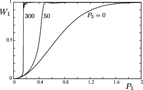
Figure 2: The probability $W_{1}(P_{1})$ of the $0\rightarrow 1$ transition for different values of the nonlinearity parameter $P_{3}=0,50,300$ from numerical simulations of Eq. (8) for $n=1$, $K_{1}=1$.

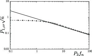
Figure 3: The rescaled critical drive parameter versus rescaled nonlinearity parameter. Solid line – theory, Eq. (10); circles – numerical simulations of Eq. (8).

The original system (4) also allows excitation from the ground state to a $N$-th energy state via a sequence of $N$ independent LZ transitions with probability

$$W=\prod_{n=1}^{N}W_{n}(P_{1},P_{3}).$$ (12)

The equation $W(P_{1},P_{3})=1/2$ defines the threshold $P_{1,LC}(P_{3})$ for this LC process. As it was found numerically Barth_2011 in the linear $P_{3}=0$ case, the product (12) quickly converges for $N\geqslant 5$ and one finds $P_{1,LC}\approx 0.79$. On the other hand, in the strongly nonlinear limit one can approximate the transition probability by the Heaviside step function $W_{n}(P_{1},P_{3})\approx H(P_{1}-P_{1,cr}(P_{3},n))$, where $P_{1,cr}$ is given by Eq. (10). Since $P_{1,cr}$ decreases with the transition number $n$ and every transition leads to nearly complete population inversion, the product (12) can be replaced by the single $n=1$ term $W\approx W_{1}$ and the capture into the LC regime occurs after the first transition. In this approximation the threshold is simplified

$$P_{1,LC}\approx P_{1,cr}(P_{3},n=1)=\frac{0.82}{\sqrt{P_{3}f_{1}K_{1}}}.$$

Note that the threshold width, defined as the inverse slope of the transition probability at $W=1/2$, equals $\Delta P_{1,LC}=0.66$ in the linear case Barth_2011 and tends to zero in the strongly nonlinear regime.

Similarly to the linear case, we can assume that the successive transitions in the nonlinear regime will be well-separated provided the time between two successive transitions satisfies $\Delta\tau\gg\tau_{AR}$, i.e., $P_{2}\gg f_{1}K_{1}P_{3}$. This estimate can be simplified because $f_{1}=\sqrt{2/\pi}/8\approx 0.1$ and we can set $K_{1}=1$. Combining the above inequality with the linear result (7) we find the condition for essentially quantum dynamics in the $P_{1,2,3}$ parameter space:

$$P_{2}\gg 1+P_{1}+0.1P_{3}.$$ (13)

This inequality together with the condition $P_{1}>P_{1,LC}$ defines the region of the parameter space, where efficient excitation of quantum states in the model (1) via the autoresonant LC is achieved.

III Semiclassical regime

If the anharmonicity parameter $P_{2}$ of the trap decreases, the two-level approximation employed in the previous section breaks down as several levels can resonate with the drive simultaneously. In the limit $P_{2}\ll 1$, the number of coupled levels is so large that the dynamics becomes semiclassical. The linear $P_{3}=0$ case in this problem was already studied in Ref. Barth_2011 . It was shown that the autoresonant excitation of BEC oscillations is possible provided the drive strength $P_{1}$ exceeds the classical autoresonance threshold for the Duffing oscillator Fajans_2001

$$P_{1,AR}=\frac{0.82}{\sqrt{P_{2}}}.$$ (14)

In this regime, the center of mass of the condensate oscillates in the trap with an increasing amplitude. The frequency of these oscillations remains close to the driving frequency during the whole excitation process, despite the variation of the driving frequency. In this section we discuss the threshold value $P_{1,AR}$ in the nonlinear case $P_{3}>0$.

Consider the Wigner representation of our problem hiley2004phase :

$$\frac{\partial f(x,p,t)}{\partial t}=\{H,f\}_{MB},$$ (15)

where $f(x,p,t)$ is the Wigner function, $H$ is the Hamiltonian

$$H=-\frac{\hbar^{2}}{2m}\frac{\partial^{2}}{\partial x^{2}}+U(x,t)+g|\Psi(x,t)|^{2}$$

and $\{H,f\}_{MB}$ denotes the Moyal bracket. Since the Moyal bracket reduces to the Poisson bracket in the semiclassical limit $\hbar\rightarrow 0$: $\{H,f\}_{MB}\approx\{H,f\}+O(\hbar^{2})$, equation (15) reduces to the Liouville equation

$$\frac{\partial f}{\partial t}+\frac{p}{m}\frac{\partial f}{\partial x}-\frac{\partial}{\partial x}\left(U+g|\Psi|^{2}\right)\frac{\partial f}{\partial p}\approx 0,$$ (16)

where in addition to the external potential $U(x,t),$ we have the self-potential $V=g|\Psi|^{2}$. This equation is reminiscent of the Vlasov equation for an ensemble of particles in the combined external and self-potentials. Note that the self-potential can be expressed via the Wigner function

$$|\Psi(x,t)|^{2}=\int_{-\infty}^{\infty}f(x,p,t)dp,$$

transforming (16) into a closed integro-differential form.

The characteristics (classical trajectories) for Eq. (16) are given by

$$\frac{d^{2}x}{dt^{2}}+\frac{1}{m}\frac{\partial U}{\partial x}+\frac{g}{m}\frac{\partial|\Psi|^{2}}{\partial x}=0.$$ (17)

Suppose one starts in a localized state, so that the Wigner function has a local maximum at the phase-space point $[x_{0},p_{0}]$. In the semiclassical limit, the Wigner function is expected to continue having a local maximum near the phase-space point $[x(t),p(t)]$ moving along the classical trajectory starting at $[x_{0},p_{0}]$. Near this point,

$$|\Psi(x+s,t)|^{2}\approx const-\kappa s^{2}/2$$

and, thus, the term $(g/m)\partial|\Psi|^{2}/\partial x$ in Eq. (17) vanishes along the trajectory of the maximum of $f$. Consequently, the nonlinearity (characterized by parameter $P_{3}$) in the semiclassical regime does not affect the evolution of the maximum. Then it also does not change the threshold of the AR (14) and should not shift the transition probability versus $P_{1}$ in contrast to the quantum regime (see Fig. 2). We confirm these conclusions in numerical simulations in the following section.

IV Numerical simulations

In this section we present numerical simulations of the original Gross-Pitaevskii equation (1) in our driven problem. We rewrite this equation in a dimensionless form using the same $\xi=x/\ell$, but a different dimensionless time $T=\omega_{0}t$:

$$i\Phi_{T} +\frac{1}{2}\Phi_{\xi\xi}-\left(\tilde{U}+Q_{3}|\Phi|^{2}\right)\Phi=0,$$ (18)

$$\tilde{U}(\xi,T) =\frac{\xi^{2}}{2}-Q_{2}\frac{\xi^{4}}{4}+Q_{1}\xi\cos\tilde{\varphi}(T),$$

where $\Phi=\sqrt{\ell}\;\Psi$, $\tilde{\alpha}=\alpha/\omega_{0}^{2}$, $Q_{1}=\sqrt{2\tilde{\alpha}}\,P_{1}$, $Q_{2}=\frac{4}{3}\sqrt{\tilde{\alpha}}\,P_{2}$, $Q_{3}=\sqrt{\tilde{\alpha}}\,P_{3}$ and $\tilde{\varphi}(T)=T-{\tilde{\alpha}\,T^{2}}/2$. The simulations are based on the standard pseudo-spectral method canuto_spectral with explicit 4-th order Runge-Kutta algorithm and adaptive step size control. The ground state of the harmonic oscillator was used as the initial condition:

$$\Phi(\xi,0)=\pi^{-1/4}\;e^{-\xi^{2}/2}.$$ (19)

The state of the condensate was analyzed by calculating its energy

$$E=\int_{-\infty}^{\infty}\left(\frac{1}{2}|\Phi_{\xi}|^{2}+\tilde{U}|\Phi|^{2}+\frac{Q_{3}}{2}|\Phi|^{4}\right)d\xi,$$

the amplitudes $c_{n}(t)$ in the basis of Hermite functions, and the Wigner distribution.

In order to study various regimes of excitation of a condensate, we performed a series of numerical simulations by varying parameters $P_{1}$ and $P_{2}$ in the linear ($P_{3}=0$) and nonlinear cases. The results of the simulations are presented in Fig. 4. The circles in the figure correspond to parameters yielding $50\%$ probability of capture into either the classical AR or the quantum LC regime.

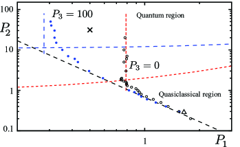
Figure 4: Different domains of phase-locking transition in the driven Gross-Pitaevskii equation (18) in the linear ($P_{3}=0$, black open circles) and nonlinear ($P_{3}=100$, filled blue circles) cases. The symbols $\times$ and $\triangle$ show parameters used in subsequent figures 6 and 7.

The classical autoresonance threshold (14) is shown by the black long-dashed line. The two roughly horizontal lines $P_{2}=1+P_{1}+0.1\,P_{3}$ separate the regions of the quantum and semiclassical dynamics in the linear ($P_{3}=0$, red line) and nonlinear ($P_{3}=100$, blue line) regimes. The vertical lines show the theoretical LC transition thresholds $P_{1,LC}$ for the linear and nonlinear regimes.

One can see that the classical AR threshold (14) yields a good approximation for the transition boundary for $P_{2}$ versus $P_{1}$ in both the linear and the nonlinear cases. In the case $P_{3}=100$, the nonlinear ladder climbing transitions emerge at significantly smaller values of the driving parameter $P_{1}$ and larger anharmonicity $P_{2}$, compared to the linear case. This is in agreement with the shift of the threshold in the nonlinear model of the autoresonant LZ transitions discussed above (see Fig. 2).

The important change due to the nonlinearity in the problem is the decrease of the width of the transition region. This effect is illustrated in Fig. 5 for the case of the semiclassical autoresonant transition. The width of the transition for the nonlinear case decreases rapidly with the increase of the nonlinearity parameter $P_{3}$ and the transition probability assumes a nearly step-like shape for $P_{3}>15$. One also observes that the threshold location, where the probability crosses $50\%$, only slightly changes with the variation of $P_{3}$ as discussed at the end of Sec. II.

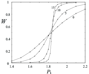
Figure 5: The transition probability versus the driving parameter $P_{1}$ for $P_{2}=0.2$ and $P_{3}=0,5,10,15$ from numerical integration of Eq.  (18).

The effect of the narrowing of the transition width in the semiclassical regime with the increase of the nonlinearity parameter can be associated with the improved stability of the autoresonant classical trajectories described by Eq. (17) . Indeed, in dimensionless variables, Eq. (17) for the characteristics of Eq. (16) becomes

$$\xi_{TT}+\xi-Q_{2}\xi^{3}+Q_{3}\frac{\partial|\Phi(\xi,T)|^{2}}{\partial\xi}+Q_{1}\cos\widetilde{\varphi}(T)=0.$$ (20)

Let the trajectory of the autoresonant maximum of the Wigner function be $\xi_{0}(T)$. The dynamics of this trajectory is described by

$$\xi_{0TT}+\xi_{0}-Q_{2}\xi_{0}^{3}+Q_{1}\cos\widetilde{\varphi}(T)=0$$ (21)

subject to $\xi_{0}=\xi_{0T}=0$ at large negative $T$ and is not affected by the nonlinearity, as described above. For studying the the evolution of a deviation $\eta=\xi-\xi_{0}(T)$ from $\xi_{0}(T)$, we linearize Eq. (20) around $\xi_{0}$ and assume $|\Phi(\xi,T)|^{2}\approx const-\kappa\eta^{2}/2$ near the maximum, to get

$$\eta_{TT}+[1-3Q_{2}\xi_{0}^{2}-\kappa Q_{3}]\eta=0.$$ (22)

We analyze the solutions of system (21), (22) in the Appendix. Numerically, in the vicinity of the threshold for $P_{3}=0$, we observe the development of instability of $\eta$. By writing $\xi_{0}=a\cos\theta$, Eq. (22) assumes the form of the Mathieu-type equation with slowly varying parameters

$$\eta_{TT}+\left\{1-\frac{3Q_{2}a^{2}}{2}-\kappa Q_{3}-\frac{3}{2}Q_{2}a^{2}\cos[2\theta(T)]\right\}\eta=0.$$ (23)

We show in the Appendix that this equation predicts parametric-type instability for $P_{3}=0$ and we attribute the existence of the width in the transition to autoresonance as seen in Fig. 5 to this effect. Note that the addition of the nonlinearity (the term $-\kappa Q_{3}$ in the last equation) shifts the eigenfrequency so that the parametric resonance can be avoided and characteristic trajectories with nearby initial conditions remain close to the classical autoresonant trajectory, narrowing the transition width as seen in Fig. 5. For the parameters in this figure, the system stabilizes at $P_{3}>0.3$ (see the Appendix). Nonetheless, the deviation from the autoresonant state is still large until $P_{3}>10$, when the autoresonant transition width practically disappears.

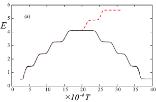
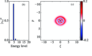
Figure 6: Numerical solutions of Eq. (18) in the LC regime for two scenarios. In the first scenario [dashed red lines in panel (a)], constant driving frequency chirp rate $\tilde{\alpha}=10^{-6}$ and $P_{1}=0.5$, $P_{2}=30$, $P_{3}=100$ (as shown by cross symbol in Fig. 4) are used. In the second scenario [solid line in panel (a)] we set $\tilde{\alpha}=0$ at $T=1.8\times 10^{5}$ and keep it constant until $T=2.2\times 10^{5}$. We restore the original value of $\tilde{\alpha}$, but with the opposite sign at $T=2.2\times 10^{5}$. The distribution of the populations of the energy levels and the Wigner quasi-probability distribution at $T=2\times 10^{5}$ for the second scenario are shown in panels (b) and (c), respectively. Here $T=\omega_{0}t=\tau/\sqrt{\tilde{\alpha}}$.

Our next numerical simulation shows that the system can be fully controlled by the AR in both the quantum and semiclassical regimes. Two protocols of such a control of the LC dynamics are shown in Fig. 6. Parameters $P_{i}$ are chosen so that both condition (13) and $P_{1}>P_{1,LC}$ are satisfied. Due to a relatively strong anharmonicity, the nonlinear LZ transitions are well separated in time. One can see that the energy in the system grows step-by-step from one energy level to another. In the first protocol, the linear frequency variation with a constant chirp rate $\alpha$ [red dashed line in Fig. 6(a)] results in the excitation of the condensate to the sixth energy level. In the second protocol (solid line) we first excite the system to the fourth energy state by decreasing driving frequency until $T=1.8\times 10^{5}$, then keep the driving frequency constant for the time span of $\Delta T=4\times 10^{4}$, and finally return the system to the ground state by increasing the driving frequency back to its original value. One can see that the quantum state of (1) can be efficiently controlled as long as the LC autoresonant conditions are met and the frequency and phase of the driving are continuous. The quantum state in the first protocol at $T=2\times 10^{5}$ is further illustrated in Figs. 6 (b) and (c) showing the distribution of populations of different levels and the Wigner function. Small deviations of the solution from the fourth eigenfunction $\chi_{4}(\xi)$ of the linear harmonic oscillator are due to the anharmonicity and the nonlinearity in the problem.

A similar control protocols for the semiclassical case are illustrated in Fig. 7. One can see that resulting wave function has a Gaussian (Poissonian in the early stages of dynamics) population distribution, characteristic of coherent states. The Wigner function is positive everywhere (on the computational grid) and close to the $n$-squeezed coherent state. The second protocol (solid line in Fig. 7) demonstrates that a more complex control scenarios are possible in the semiclassical case, as long as the driving parameter is within the region of autoresonant dynamics and the driving phase and frequency are continuous functions of time.

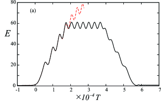
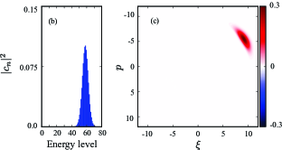
Figure 7: The numerical solutions of Eq. (18) in the semiclassical regime for parameters $\tilde{}\alpha=10^{-6}$, $P_{1}=1.6$, $P_{2}=0.3$, $P_{3}=100$ (represented by the triangle in Fig. 4). In the second scenario (solid line) the frequency chirp is set to zero from $T=1.8\times 10^{4}$, but restored to the original value with opposite sign at $T=3.8\times 10^{4}$. The distribution of populations of energy levels and the Wigner function at $T=2.8\times 10^{4}$ for the second scenario are shown in panels (b) and (c), respectively.

V Conclusions

In conclusion, we have studied the effect of the particles interaction on the excitation of Bose-Einstein condensate in a anharmonic trap under chirped-frequency perturbation. We have identified three dimensionless parameters $P_{1,2,3}$ [see Eqs. (3)] characterizing the driving strength, the anharmonicity and the strength of the interaction to show that there exist two very different regimes of excitation in this parameters space, i.e., the quantum-mechanical ladder climbing (LC) and the semiclassical autoresonance (AR). The transition boundary to the semiclassical AR in the $P_{1,2}$ parameter space is independent of the nonlinearity parameter $P_{3}$. In contrast, the LC transition boundary is significantly affected by the strength of the interaction of the particles, because the underlying nonlinear Landau-Zener (LZ) transitions behave differently than their linear counterpart. In the limit of strong interaction, the nonlinear LZ transition probability as a function of the driving strength parameter $P_{1}$ approaches the Heaviside step function due to the nonlinear phase-locking. We have also found that in both the quantum and the semiclassical regimes the width $\Delta P_{1}$ of the transition decreases as the strength of the interaction increases. In the quantum limit this effect is related to the autoresonance of the nonlinear LZ transitions, while in the semiclassical limit, the effect is due to the wave packet stability enhancement by avoiding parametric resonance between the center-of-mass motion and the internal dynamics of the condensate.

Possible applications of the results of this paper may include a control of the quantum state of BECs and the implementation of precision detectors based on either the LC or the AR. Unlike the noninteracting case Murch_2010 , the resolution of such a detector is not limited by quantum fluctuations if the particles interaction is strong enough.

APPENDIX: Stability of autoresonant trajectories.

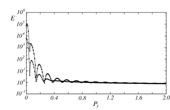
Figure 8: The energy $E=\frac{1}{2}\left\langle\eta_{T}^{2}+\eta\right\rangle$ averaged over the integration time versus $P_{3}$ from the numerical solution of Eqs. (20),(23) near the threshold of the autoresonance. The lines with squares and circles correspond to $\alpha=10^{-4}$ and $\alpha=10^{-6}$, respectively.

Here we discuss the Mathieu-type Eq. (23)

$$\eta_{TT}+[B-C\cos(2\theta)]\eta=0,$$ (24)

where $B=1-\frac{3Q_{2}a^{2}}{2}-\kappa Q_{3}$, $C=\frac{3}{2}Q_{2}a^{2}$, describing the deviation $\eta$ of the trajectory from the autoresonant solution $\xi_{0}=a\;\cos\theta$ given by Eq. (21).

For sufficiently small amplitudes $a$ this solution is described by Scholarpedia

$$\frac{{da}}{dT} = (Q_{1}/2)\sin\Phi,$$ (25)

$$\frac{{d\Phi}}{dT} = \alpha T-(3Q_{2}/8)a^{2}+(Q_{1}/2a)\cos\Phi,$$ (26)

where $\Phi=\theta-\widetilde{\varphi}+\pi$ is the phase mismatch, which starts at zero initially (at large negative $t$, where $a$ is also zero). We are interested in passage through resonance when parameter $Q_{1}$ is close to the autoresonance threshold $Q_{1th}$ (from either above or below). In both of these cases,  $\Phi$ slowly increases initially and then passes $\pi/2$. Then when slightly above the threshold, $\Phi$ starts oscillating, but remains bounded ($|\Phi|<\pi$), while below the threshold $\Phi$ continues to increase reaching $\pi$ and the oscillator fully dephases from the drive.

At this point we observe that there are three parameters ($\alpha,Q_{1},Q_{2}$) in system (25), (26). However, by introducing the slow time $\tau={\alpha^{1/2}T}$ and rescaled amplitude $A=\sqrt{3/8}$ $\alpha^{-1/4}Q_{2}^{1/2}a$ we obtain a single parameter system

$$\frac{{dA}}{d\tau} = \mu\sin\Phi,$$ (27)

$$\frac{{d\Phi}}{d\tau} = \tau-A^{2}+(\mu/A)\cos\Phi,$$ (28)

where

$$\mu=\sqrt{\frac{3}{32}}Q_{1}Q_{2}^{1/2}{\alpha^{-3/4}.}$$ (29)

The autoresonant threshold in this system is $\mu_{th}=0.41$ Scholarpedia , which upon the return to the original parameters $P_{1,2}$ yields (14). Note that at the threshold ($\mu=\mu_{th}$) the rescaled problem has no free parameters.

Next we discuss Eq. (24). Here, using (26), we have

$$\frac{{d\theta}}{dT}=\frac{{d}\widetilde{\varphi}}{{dT}}+\frac{d\Phi}{dT}=1-\alpha T+\frac{d\Phi}{dT}=1-\frac{3}{8}Q_{2}a^{2}+\frac{Q_{1}}{2a}\cos\Phi$$ (30)

and assume that $S=-\frac{3}{8}Q_{2}a^{2}+\frac{Q_{1}}{2a}\cos\Phi$ is small compared to unity in the region of dephasing. This suggests to transform from $T$ to $\theta$ in (24) and approximate the problem by the Mathieu equation with slow coefficients

$$\frac{{d^{2}\eta}}{{d\theta^{2}}}+[B^{\prime}-C^{\prime}\cos(2\theta)]\eta\approx 0$$ (31)

where to lowest order in small parameters

$$B^{\prime} = \frac{B}{(1+S)^{2}}\approx 1-\frac{3}{4}Q_{2}a^{2}-\frac{Q_{1}}{a}\cos\Phi-\kappa Q_{3}$$ (32)

$$C^{\prime} = \frac{C}{(1+S)^{2}}\approx C=\frac{3}{2}Q_{2}a^{2}$$ (33)

From the theory of the Mathieu equation (with fixed parameters, which we assume locally in our case), the stability condition of the solution of (31) is Hayashi

$$B^{\prime}<1-C^{\prime}/2$$ (34)

or

$$\kappa Q_{3}>\max\left(-\frac{Q_{1}}{a}\cos\Phi\right).$$ (35)

Finally, in the last equation we use the rescaled amplitude $A$ instead of $a$ to get the dimensionless condition

$$\kappa P_{3}>P_{1}P_{2}^{1/2}\max\left(-\frac{\cos\Phi}{A}\right)_{\mu=\mu_{th}}$$ (36)

where the rescaled parameters are $P_{1}=Q_{1}/(2{\alpha)^{1/2}}$, $P_{2}=(3/4)Q_{2}/{\alpha^{1/2}}$, $P_{3}=Q_{3}/{\alpha^{1/2}}$ and the value of $\max\left(-\frac{\cos\Phi}{A}\right)_{\mu=\mu_{th}}=0.37$ is found numerically by solving (27), (28). Thus, for $\kappa=0$, the solution remains stable only if $\Phi<\pi/2$ and, since we approach this value in the vicinity of the threshold as mentioned above, one encounters instability near the threshold, explaining the appearance of the width of the autoresonant transition as some initial conditions dephase. On the other hand, a sufficiently large $\kappa P_{3}$ stabilizes the solution and the width of the autoresonance threshold disappears. For the parameters of Fig. 5 one finds that the solution is stable for $P_{3}>0.27$. Finally we check these conclusions by solving the set (21) and (22) numerically. The results of these simulations are presented in Fig. 8, showing the energy $E=\frac{1}{2}\left\langle\eta_{T}^{2}+\eta\right\rangle$ averaged over the integration time versus $P_{3}$ for the parameters of Fig. 5 and initial conditions $\eta=1$, $\eta_{T}=0$ and integrating between $T=-2\times 10^{4}$ and $4\times 10^{4}$ for $\alpha=10^{-4\text{ }}$and $T=-2\times 10^{5}$ and $4\times 10^{5}$ for $\alpha=10^{-6}$. One can see the transition to instability at $P_{3}<0.3$.

References

- (1) J. F. Dobson, Phys. Rev. Lett., 73, 2244 (1994).
- (2) H. Ott, J. Fortágh, S. Kraft, A. Günther, D. Komma, and C. Zimmermann, Phys. Rev. Lett., 91, 040402 (2003).
- (3) V. I. Veksler, Doklady Akad. Nauk SSSR, 43, 346 (1944); E. M. McMillan, Phys. Rev., 68, 144 (1945).
- (4) L. Friedland, Physical Review E, 59, 4106 (1999).
- (5) L. Friedland and A. G. Shagalov, Physics of Fluids, 14, 3074 (2002).
- (6) M. Assaf and B. Meerson, Phys. Rev. E, 72, 016310 (2005).
- (7) J. Fajans, E. Gilson, and L. Friedland, Phys. Rev. Lett., 82, 4444 (1999).
- (8) R. R. Lindberg, A. E. Charman, J. S. Wurtele, L. Friedland, and B. A. Shadwick, Physics of Plasmas, 13, 123103 (2006).
- (9) O. Yaakobi, L. Friedland, R. R. Lindberg, A. E. Charman, G. Penn, and J. S. Wurtele, Physics of Plasmas, 15, 032105 (2008).
- (10) L. A. Kalyakin, M. A. Shamsutdinov, R. N. Garifullin, and R. K. Salimov, The Physics of Metals and Metallography, 104, 107 (2007).
- (11) S. V. Batalov and A. G. Shagalov, The Physics of Metals and Metallography, 114, 103 (2013).
- (12) G. Klughertz, L. Friedland, P.-A. Hervieux, and G. Manfredi, Phys. Rev. B, 91, 104433 (2015).
- (13) A. Barak, Y. Lamhot, L. Friedland, and M. Segev, Phys. Rev. Lett., 103, 123901 (2009).
- (14) G. Marcus, L. Friedland, and A. Zigler, Phys. Rev. A, 69, 013407 (2004).
- (15) L. Friedland, The Astrophysical Journal, 547, L75 (2001).
- (16) A. I. Nicolin, M. H. Jensen, and R. Carretero-Gonzalez, Physical Review E, 75, 036208 (2007).
- (17) R. Bücker, T. Berrada, S. van Frank, J.-F. Schaff, T. Schumm, J. Schmiedmayer, G. Jäger, J. Grond, and U. Hohenester, J. Phys. B: At. Mol. Opt. Phys., 46, 104012 (2013).
- (18) F. Dalfovo, S. Giorgini, L.P. Pitaevskii, and S. Stringari Rev. Mod. Phys., 71, 463 (1999).
- (19) I. Barth, L. Friedland, O. Gat, and A. G. Shagalov, Phys. Rev. A, 84, 013837 (2011).
- (20) G. B. Andresen, M. D. Ashkezari, M. Baquero-Ruiz et al, Phys. Rev. Lett., 106 025002 (2011).
- (21) Y. Shalibo, Y. Rofe, I. Barth, L. Friedland, R. Bialczack, J. M. Martinis, and N. Katz, Phys. Rev. Lett., 108, 037701 (2012).
- (22) L. Landau and E. Lifshits, Quantum Mechanics: Non-relativistic Theory (Butterworth-Heinemann, 1977).
- (23) L. Landau, Phys. Z. Sowietunion, 2, 46 (1932); C. Zener, Proceedings of the Royal Society A: Mathematical, Physical and Engineering Sciences, 137, 696 (1932).
- (24) N. V. Vitanov and B. M. Garraway, Phys. Rev. A, 53, 4288 (1996).
- (25) J. Liu, L. Fu, B.-Y. Ou, S.-G. Chen, D.-I. Choi, B. Wu, and Q. Niu, Phys. Rev. A, 66, 023404 (2002).
- (26) Q. Zhang, P. Hänggi, and J. Gong, New Journal of Physics, 10, 073008 (2008).
- (27) F. Trimborn, D. Witthaut, V. Kegel, and H. J. Korsch, New Journal of Physics, 12, 053010 (2010).
- (28) B. Wu and Q. Niu, Phys. Rev. A, 61, 023402 (2000).
- (29) O. Zobay and B. M. Garraway, Phys. Rev. A, 61, 033603 (2000).
- (30) J. Fajans and L. Friedland, Am. J. Phys., 69, 1096 (2001).
- (31) B. Hiley, in Proc. Int. Conf. Quantum Theory: Reconsid- eration of Foundations, Vol. 2 (2004) pp. 267.
- (32) C. Canuto, M. Y. Hussaini, A. M. Quarteroni, and T. A. Zang, Spectral methods (Springer-Verlag, Berlin, 2006).
- (33) K. W. Murch, R. Vijay, I. Barth, O. Naaman, J. Aumentado, L. Friedland, and I. Siddiqi, Nat. Phys, 7, 105 (2010).
- (34) L. Friedland, Scholarpedia 4, 5473 (2009).
- (35) C. Hayashi, Nonlinear Oscillations in Physical Systems (Princeton University Press, Princeton, 1985).