Type III Solar Radio Burst Source Region Splitting Due to a Quasi-Separatrix Layer

Abstract

We present low-frequency (80–240 MHz) radio imaging of type III solar radio bursts observed by the Murchison Widefield Array (MWA) on 2015/09/21. The source region for each burst splits from one dominant component at higher frequencies into two increasingly-separated components at lower frequencies. For channels below $\sim$132 MHz, the two components repetitively diverge at high speeds (0.1–0.4 c) along directions tangent to the limb, with each episode lasting just $\sim$2 s. We argue that both effects result from the strong magnetic field connectivity gradient that the burst-driving electron beams move into. Persistence mapping of extreme ultraviolet (EUV) jets observed by the Solar Dynamics Observatory reveals quasi-separatrix layers (QSLs) associated with coronal null points, including separatrix dome, spine, and curtain structures. Electrons are accelerated at the flare site toward an open QSL, where the beams follow diverging field lines to produce the source splitting, with larger separations at larger heights (lower frequencies). The splitting motion within individual frequency bands is interpreted as a projected time-of-flight effect, whereby electrons traveling along the outer field lines take slightly longer to excite emission at adjacent positions. Given this interpretation, we estimate an average beam speed of 0.2 c. We also qualitatively describe the quiescent corona, noting in particular that a disk-center coronal hole transitions from being dark at higher frequencies to bright at lower frequencies, turning over around 120 MHz. These observations are compared to synthetic images based on the Magnetohydrodynamic Algorithm outside a Sphere (MAS) model, which we use to flux-calibrate the burst data.

1. Introduction

Type III solar radio bursts are among the principal signatures of magnetic reconnection, the process thought to underlie solar flares. Their high brightness temperatures demand a coherent, nonthermal emission mechanism that is generally attributed to plasma emission stimulated by semi-relativistic electron beams. Electrons accelerated at the reconnection site generate Langmuir waves (plasma oscillations) in the ambient plasma through the bump-on-tail beam instability. Those Langmuir waves then shed a small fraction of their energy in radio emission near the fundamental plasma frequency ($f_{p}$) or its second harmonic. This theory was proposed by Ginzburg & Zhelezniakov (1958) and has since been developed by many authors (see reviews by Robinson & Cairns 2000; Melrose 2009).

Radio bursts are classified by their frequency drift rates, and type IIIs are so named because they drift faster than types I and II (Wild & McCready, 1950). A recent review of type III literature is provided by Reid & Ratcliffe (2014). Starting frequencies are typically in the 100s of MHz, and because the emission frequency is proportional to the square of the ambient electron density ($f_{p}~{}\propto{}~{}\sqrt{n_{e}}$), standard type III radiation drifts to lower frequencies as the accelerated electrons stream outward. Coronal type III bursts refer to those that drift down to tens of MHz or higher. Beams that escape along open field lines may continue to stimulate Langmuir waves in the solar wind plasma, producing interplanetary type III bursts that may reach 20 kHz and below around 1 AU and beyond. We will focus on coronal bursts for which some fraction of the electrons do escape to produce an interplanetary type III.

X-ray flares and type III bursts have been linked by many studies. Various correlation rates have been found, with a general trend toward increased association with better instrumentation. Powerful flares ($\geq{}$C5 on the GOES scale) almost always generate coherent radio emission, generally meaning a type III burst or groups thereof (Benz et al., 2005, 2007). Weaker flares may or may not have associated type IIIs depending on the magnetic field configuration (Reid & Vilmer, 2017), and type IIIs may be observed with no GOES-class event if, for instance, the local X-ray production does not sufficiently enhance the global background (Alissandrakis et al., 2015). Flares that produce X-ray or extreme ultraviolet (EUV) jets are frequently associated with type III emission (Aurass et al., 1994; Kundu et al., 1995; Raulin et al., 1996; Trottet, 2003; Chen et al., 2013b; Innes et al., 2016; Mulay et al., 2016; Hong et al., 2017; Cairns et al., 2017). Such jets are collimated thermal plasma ejections that immediately follow, are aligned with, and are possibly heated by the particle acceleration responsible for radio bursts (Saint-Hilaire et al., 2009; Chen et al., 2013a). We will exploit the alignment between EUV jets and type III electron beams to develop an understanding of radio source region behavior that, to our knowledge, has not been previously reported.

This is the first type III imaging study to use the full 128-tile Murchison Widefield Array (MWA; Lonsdale et al. 2009; Tingay et al. 2013b), which follows from type III imaging presented by Cairns et al. (2017) using the 32-tile prototype array. The MWA’s primary science themes are outlined by Bowman et al. (2013), and potential solar science is further highlighted by Tingay et al. (2013a). The first solar images using the prototype array and later the full array are detailed by Oberoi et al. (2011) and Oberoi et al. (2014), respectively. Suresh et al. (2016) present a statistical study of single-baseline dynamic spectra, which exhibit the lowest-intensity solar radio bursts ever reported. We present the first time series imaging.

Along with the Low Frequency Array (LOFAR; van Haarlem et al. 2013; Morosan et al. 2014), the MWA represents a new generation of low frequency interferometers capable of solar imaging. Previous imaging observations at the low end of our frequency range were made by the decommissioned Culgoora (Sheridan et al., 1972, 1983) and Clark Lake (Kundu et al., 1983) radioheliographs, along with the still-operational Gauribidanur Radioheliograph (Ramesh et al., 1998, 2005). The high end of the MWA’s frequency range overlaps with the Nançay Radioheliograph (NRH; Kerdraon & Delouis 1997), which has facilitated a number of type III studies referenced here.

This paper is structured as follows. §2 describes our observations and data reduction procedures. Our analyses and results are detailed in §3. §3.1 considers the quiescent corona outside burst periods, which we compare to synthetic images used to flux calibrate the burst data in §3.2. §3.3 characterizes the type III source region structure and motion, and the local magnetic field configuration is inferred using EUV observations in §3.4. In §4, our results are combined to produce an interpretation of the radio source region behavior. §5 provides concluding remarks.

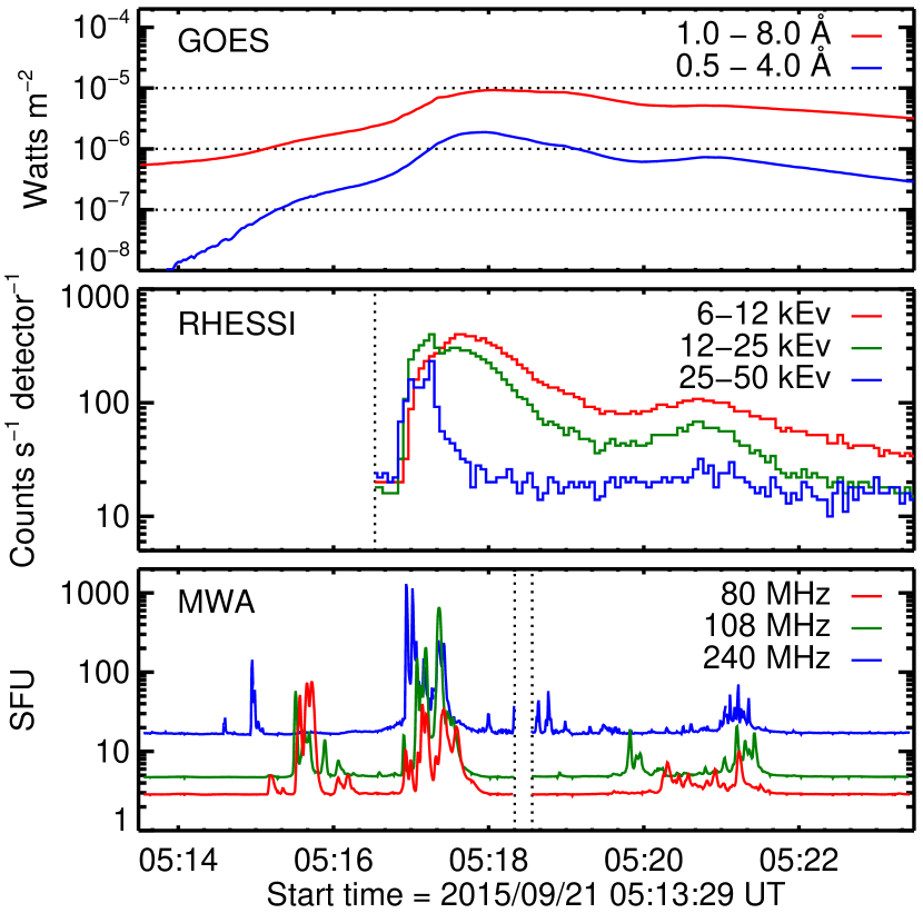
Figure 1.— Top: GOES soft X-ray light curves, showing the C8.8 flare that peaked at 05:18 UT. Dotted lines from bottom to top indicate the B, C, and M-class thresholds. Middle: RHESSI count rates from 6–50 kEv. The dotted line indicates the end of RHESSI’s night (Earth-eclipse) period. Bottom: MWA light curves at 80, 108, and 240 MHz. Dotted lines indicate the transition between continuous observing periods.

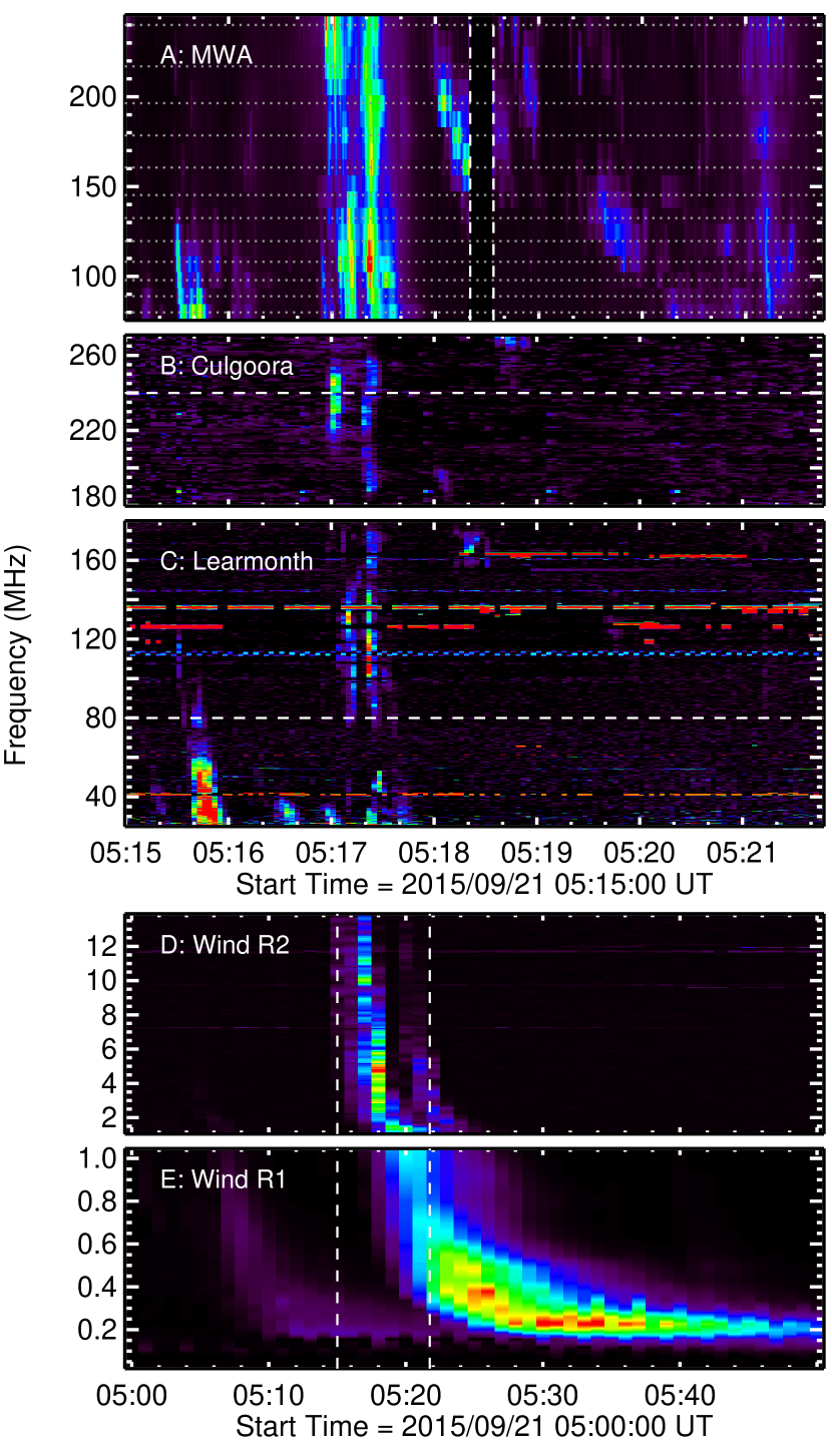
Figure 2.— MWA dynamic spectrum (DS) produced from total image intensities and interpolated to a spectral resolution equal to the minimum separation between observing bandwidths (see §2.1.) Dashed vertical lines indicate the transition between continuous observing periods, and dotted horizontal lines mark the 12, 2.56 MHz-wide frequency channels. Culgoora and Learmonth DS. Dashed lines indicate the MWA frequency coverage bounds (80–240 MHz). Wind/WAVES RADS. Note that the time axis is expanded to show the low-frequency tail. The dashed All DS are log-scaled and then background-subtracted. A corresponding movie is available in the online material.

2. Observations

We focus on a brief series of type III bursts associated with a C8.8 flare that peaked at 05:18 UT on 2015/09/21. The flare occurred in Active Region 12420 on the east limb. This investigation began by associating MWA observing periods that utilize the mode described in §2.1 with isolated type III bursts logged in the National Oceanic and Atmospheric Administration (NOAA) solar event reports. A small sample of bursts detected from 80 to 240 MHz were selected, and we chose this event for a case study because of the unusual source structure and motion. A survey of other type III bursts is ongoing.

Figure 1 shows the soft X-ray (SXR) light curves from the Geostationary Operational Environmental Satellite (GOES) for our MWA observation period, along with those from the Reuven Ramaty High-Energy Solar Spectroscopic Imager (RHESSI; Lin et al. 2002). The corresponding MWA light curves, as derived in §2.1 and §3.1, show that the radio bursts occur primarily around the hard X-ray (HXR, 25–50 keV) peak and just before the SXR peak, with some minor radio bursts scattered throughout the SXR rise and decay phases. HXR and type III emissions are known to be approximately coincident in time (Arzner & Benz, 2005) and are generally attributed to oppositely-directed particle acceleration, with HXR production resulting from heating by the sunward component. The same process may underlie both, however small differences in the timing, along with large differences in the requisite electron populations, suggest there may be multiple related acceleration processes (e.g. Brown & Melrose 1977; Krucker et al. 2007; White et al. 2011; Cairns et al. 2017). In contrast, SXR emission is associated with thermal plasma below the reconnection site, generally peaking somewhat later with a more gradual profile as in Figure 1.

Our initial radio burst detections relied on observations from the Learmonth and Culgoora solar radio spectrographs. Part of the global Radio Solar Telescope Network (RSTN; Guidice et al. 1981), the Learmonth spectrograph covers 25 to 180 MHz in two 401-channel bands that run from 25–75 and 75–180 MHz. Additional technical details are provided by Kennewell & Steward (2003). The Culgoora spectrograph (Prestage et al., 1994) has broader frequency coverage (18–1800 MHz) over four 501-channel bands. Only the 180–570 MHz band is relevant here, and we show just a portion of it because the Learmonth spectrograph is more sensitive where they overlap. Both instruments perform frequency sweeps every 3 s. Dynamic spectra are plotted in Figure 2, each being log-scaled and background-subtracted by 5-min boxcar averages.

Figure 2 also includes rom the Radio and Plasma Wave Investigation (WAVES; Bougeret et al. 1995) on the Wind spacecraft. These data demonstrate an interplanetary component to the coronal type III bursts, which requires there be connectivity to open field lines along which electrons escaped the corona. This will be important to our interpretation of the magnetic field configuration in §4.

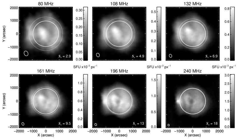
Figure 3.— MWA Stokes I images for 6 of the 12 frequency bands during a quiescent period at 2015/09/21 05:13:33.20 UT. The solid inner circles denote the optical disk, and the dotted outer circles denote the Newkirk-model (Newkirk, 1961) limb for a given frequency. Ellipses in the bottom-left corners represent the synthesized beams. Values in the bottom-right corners are full-Sun integrated flux densities ($S_{\nu}$) in SFU, and the color bars represent the flux density enclosed by each ixel in SFU$\times{}10^{-3}$ (see §3.2 for details). A movie showing the full time series for all 12 bands is available in the online material.

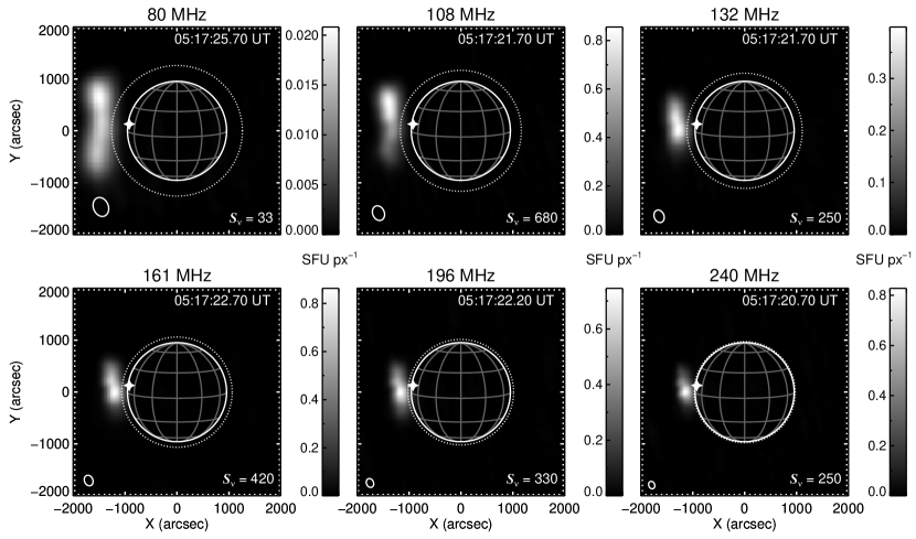
Figure 4.— Same as Fig. 3 but for the . Color bar units n SFUtars mark the X-ray flare site.

2.1. Murchison Widefield Array (MWA)

The MWA is a low-frequency radio interferometer in Western Australia that consists of 128 aperture arrays (“tiles”), each comprised of 16 dual-polarization dipole antennas (Tingay et al., 2013b). It has an instantaneous bandwidth of 30.72 MHz that can be spread flexibly from 80 to 300 MHz. Our data employ a “picket fence” observing mode, whereby twelve 2.56 MHz bands are distributed between 80 and 240 MHz with gaps of 9–23 MHz between them. This configuration is chosen to maximize spectral coverage while avoiding radio frequency interference (RFI). Data are recorded with a time resolution of 0.5 s and a spectral resolution of 40 kHz, which we average across the 2.56 MHz bandwidths to produce images centered at 80, 89, 98, 108, 120, 132, 145, 161, 179, 196, 217, and 240 MHz. Figures 3 and 4 show images at six frequencies during quiescent and burst phases, respectively, and a movie showing all twelve bands over the full time series is available in the online material.

Visibilities were produced using the standard MWA correlator (Ord et al., 2015) and cotter (Offringa et al., 2015). For our calibrator observations, this included 8-s time averaging and RFI flagging using the aoflagger algorithm (Offringa et al., 2012). RFI flagging was disabled for the solar observations, as it tends to flag out burst data. Calibration solutions for the complex antenna gains were obtained with standard techniques (Hurley-Walker et al., 2014) using observations of a bright and well-modelled calibrator source (Centaurus A) made $\sim$2 hours after the solar observations. To improve the calibration solutions, the calibrator was imaged and ten loops of self-calibration were performed in the manner described by Hurley-Walker et al. (2017).

This last step is typically performed on science target images, but we apply it instead to the calibrator for two reasons. First, we find that day-time observations generally produce inferior calibration solutions compared to analogous night-time data. We attribute this to contamination of the calibrator field by sidelobe emission from the Sun, but ionospheric and temperature effects may also be important. Second, the clean algorithm essential to the self-calibration process works best when the field is dominated by compact, point-like sources, which is not the case for the Sun. The same steps performed on our solar images tended to degrade the overall quality of the calibration solutions and bias the flux distribution of the final images. However, we find that it is best to self-calibrate on the field source to obtain quality polarimetry because transferring calibration solutions from a lower-elevation pointing typically produces overwhelming Stokes I leakage into the other Stokes portraits. For this reason, we do not include polarimetry here. Progress has been made on producing reliable polarimetric images of the Sun with the MWA, as well as improving the dynamic range, but that is beyond the scope of this paper.

Once calibrated, imaging for each 0.5 s integration is accomplished using WSClean (Offringa et al., 2014) with the default settings except where noted below. Frequencies are averaged over each 2.56 MHz bandwidth, excluding certain fine channels impacted by instrumental artefacts. To emphasize spatial resolution, we use the Briggs -2 weighting scheme (Briggs, 1995). Cleaning is performed with $\sim$10 pixels across the synthesized beam, yielding 16–36$\arcsec$ px^-1 from 240–80 MHz. We use a stopping threshold of 0.01, which is roughly the average RMS noise level in arbitrary units obtained for quiescent images cleaned with no threshold. Major clean cycles are used with a gain of 0.85 (-mgain 0.85), and peak finding uses the quadrature sum of the instrumental polarizations (-joinpolarizations). Finally, Stokes I images are produced using the primary beam model described by Sutinjo et al. (2015).

To compare MWA data with other solar imaging observations, we introduce the mwa_prep routine, now available in the SolarSoftWare libraries for IDL (SSW, Freeland & Handy 1998). WSClean and the alternative MWA imaging tools produce FITS images using the sin-projected celestial coordinates standard in radio astronomy. Solar imaging data typically use “helioprojective-cartesian” coordinates, which is a tan projection aligned to the solar rotation axis with its origin at Sun-center (Thompson, 2006). To convert between the two coordinate systems, mwa_prep rotates the image about Sun-center by the solar P angle, interpolates onto a slightly different grid to account for the difference between the sin and tan projections, and scales the images to a uniform spatial scale (20$\arcsec$ px^-1). By default, the final images are cropped to 6$\times$6 $\rm{R}_{\odot}$, yielding 289$\times$289 pixels. FITS headers are updated accordingly, after which the various SSW mapping tools can be used to easily overplot data from different instruments.

We will consider quiescent radio structures in §3.1 against corresponding model images that are used for flux calibration in §3.2. Burst structure and dynamics are discussed in §3.3.

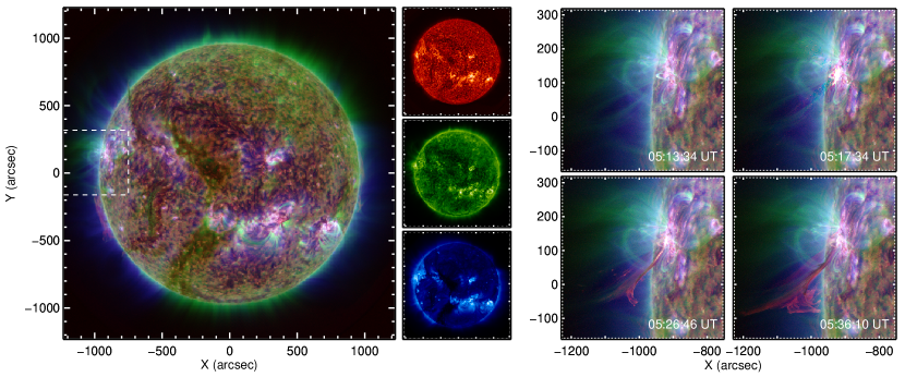
Figure 5.— An overview of the event seen by SDO/AIA using RGB composites of the 304, 171, and 211 Å channels. The top panels on the right half show nearly the same times as Figs. 3 (left) and 4 (right), with the rightmost panel corresponding to just before the SXR peak. The bottom-right panels show snapshots of the EUV jets that follow the radio bursts.

2.2. Solar Dynamics Observatory (SDO)

The Solar Dynamics Observatory (SDO, Pesnell et al. 2012) is a satellite with three instrument suites, of which we use the Atmospheric Imaging Assembly (AIA; Lemen et al. 2012). We also indirectly use photospheric magnetic field observations from the Helioseismic and Magnetic Imager (HMI; Scherrer et al. 2012), which inform the synthetic images in §3.1. The AIA is a full-Sun imager consisting of four telescopes that observe in seven narrowband EUV channels with a 0.6″ px^-1 spatial resolution and 12 s cadence, along with three UV bands with a lower cadence.

Calibrated (“level 1”) data are obtained from the Virtual Solar Observatory (VSO, Hill et al. 2009). The SSW routine aia_deconvolve_richardsonlucy is used to deconvolve the images with filter-specific point spread functions, and aia_prep is used to co-align and uniformly scale data from the different telescopes. Figure 5 presents an overview of our event using RGB composites of the 304, 171, and 211 Å channels. These bands probe the chromosphere, upper transition region / low corona, and corona, respectively, with characteristic temperatures of .05 (He II), 0.63 (Fe IX), and 2 MK (Fe XIV).

The AIA observations show a fairly compact flare that produces several distinct EUV jets beginning just before the soft X-ray peak at 05:18 UT. This includes higher-temperature material visible in up to the hottest band (94 Å, 6.3 MK), along with cooler ejecta at chromospheric temperatures that appears in emission at 304 Å and in absorption at other wavelengths. These outflows reveal a complex magnetic field configuration south of the flare site, which we will explore in §3.4 and in §4 with respect to the radio emission.

3. Analysis & Results

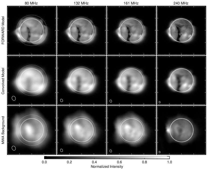
Figure 6.— Top: Expected free-free and gyroresonance emission at four frequencies predicted by FORWARD based on the MAS thermodynamic MHD model. Middle: Model image convolved with the corresponding MWA beams. Bottom: Median MWA emission outside burst periods over the first 4-min observation period, which is assumed to be the quiescent background for flux calibration. Plot axes and annotations are as in Fig. 3. An animation with all 12 channels is available in the online material.

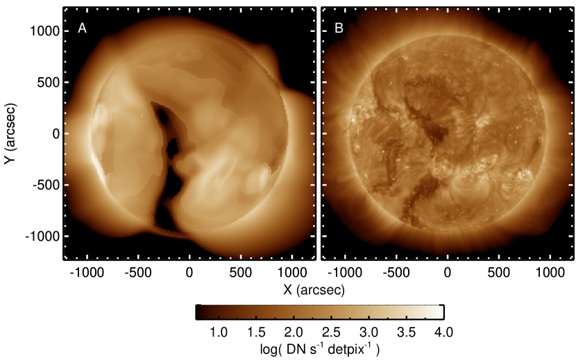
Figure 7.— 193 Å synthetic image (A) and SDO observation (B). The synthetic image applies the telescope response function so that both images are plotted on exactly the same scale in instrumental units (DN) per sec per detector pixel (detpix).

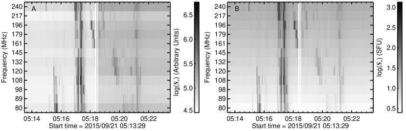
Figure 8.— Uncalibrated (A) and flux-calibrated (B) dynamic spectra generated from total image intensities. The Y axes intervals are not uniform; values refer to the 12 2.56-MHz-wide observing bandwidths separated by gaps of 9–23 MHz (see §2.1). An interpolated dynamic spectrum with a uniform Y axis is shown in Fig 2.

3.1. Quiescent Structure & Model Comparison

We examine model images of the coronal intensity at MWA frequencies to qualitatively compare the expected and observed structures outside of burst periods. In the next subsection, we also use the predicted quiescent flux densities to obtain a rough flux calibration of our burst data. Synthetic Stokes I images are obtained using FORWARD, an SSW package that can generate a variety of coronal observables using different magnetic field and/or thermodynamic models. At radio wavelengths, FORWARD computes the expected contributions from thermal bremsstrahlung (free-free) and gyroresonance emission based on the modeled temperature, density, and magnetic field structure. Details on those calculations, along with the package’s other capabilities, are given by Gibson et al. (2016).

Our implementation uses the Magnetohydrodynamic Algorithm outside a Sphere (MAS; Lionello et al. 2009) medium resolution (hmi_mast_mas_std_0201) model. The MAS model combines an MHD extrapolation of the coronal magnetic field (e.g. Mikić et al. 1999) based on photospheric magnetogram observations from the HMI with a heating model adapted from Schrijver et al. (2004). Comparisons between MAS-predicted images and data have been made a number of times for EUV and soft X-ray observations, with generally good agreement for large-scale structures (e.g. Riley et al. 2011; Reeves & Golub 2011; Downs et al. 2012). We make the first radio comparisons.

The top row of Figure 6 shows synthetic images at four MWA frequencies. Beam-convolved versions are shown in the middle row, but note that this does not account for errors introduced by the interferometric imaging process, such as effects related to deconvolving a mixture of compact and diffuse emission or to nonlinearities in the clean algorithm. MWA data are shown in the bottom row and reflect median pixel values over the first five-minute observation (05:13:33 to 05:18:20), excluding burst periods defined as when the total image intensities exceed 105% of the first 0.5 s integrations for each channel. An animation with all 12 channels is available in the online material. For context, we also show a comparison of a 193 Å SDO observation and prediction using the same model in Figure 7.

The agreement between the observed and modelled radio images is best at our highest frequencies ($\gtrsim$ 179 MHz), where the correspondence is similar to that of the EUV case. For both, the model reproduces structures associated with coronal holes near the central meridian and the large active region complexes in the southwest. The large-scale structure associated with the southern polar coronal hole is also well-modelled for the radio case. A similar structure is predicted for the EUV but is disrupted by the observed polar plumes in the manner described by Riley et al. (2011). The modelled images also under-predict emission from EUV coronal holes, which may be due to contributions from low-temperature ($<$ 500,000 K) material ignored by the emissivity calculations. Other contributing factors might be inaccuracies in the heating model, evolution of the magnetic boundary from that used for the simulation, or 193 Å emission from non-dominant ions formed at low temperatures.

A number of discrepancies between the model and MWA observations are also apparent, particularly with decreasing frequency. With the exception of the bright region on the east limb at 240 MHz, which we will revisit in §4, we suspect these differences underscore the importance of propagation effects to the appearance of the corona at low frequencies. In particular, refraction (ducting) of radio waves as they encounter low-density regions, as well as scattering by density inhomogeneities, can profoundly alter the observed source structure (see reviews by Lantos 1999; Shibasaki et al. 2011). Both effects can increase a source’s spatial extent, decrease its brightness, and alter its apparent location (e.g. Aubier et al. 1971; Alissandrakis 1994; Bastian 1994; Thejappa & MacDowall 2008; Ingale et al. 2015). We likely see the effects of scattering and/or refraction in the increased radial extent of the observed emission at all frequencies compared to the beam-convolved model images, though an enhanced density profile may also contribute. Likewise, these propagation effects may be responsible for dispersing the signatures of the southwestern active regions, which are prominent in the synthetic images but only barely discernible in our observations.

Most conspicuously, the disk-center coronal hole gradually transitions from a dark feature at high frequencies to a bright one at low frequencies in the observations but not in the synthetic data. This could be due to the diminished spatial resolution at low frequencies, meaning the coronal hole signature is swamped by emission from the bright region to the northeast. However, that effect should serve only to reduce the coronal hole contrast, as it does for the beam-convolved synthetic images. Indeed, another set of observations of a different disk-center coronal hole also show this dark-to-bright transition from high to low frequencies with even less ambiguity. In both cases, the transition is gradual and turns over around 120 MHz. Above the $\sim$120 MHz transition we observe, coronal holes are consistently reported as intensity depressions (e.g. Mercier & Chambe 2012), which is expected given their low densities. At longer wavelengths, coronal holes have sometimes been seen in emission (Dulk & Sheridan, 1974; Lantos et al., 1987), as in our lower frequency channels. Again, scattering (Riddle, 1974; Hoang & Steinberg, 1977) and/or refraction (Alissandrakis, 1994) may be able to explain low-frequency enhancements in low-density regions, but a satisfactory explanation has not been achieved, in part because of limited data. The MWA appears to be uniquely poised to address this topic given that the transition of certain coronal holes between being dark or bright features occurs within the instrument’s frequency range, but an analysis of this is beyond the scope of this paper.

3.2. Flux Calibration

Absolute flux calibration is challenging for radio data because of instrumental uncertainties and effects related to interferometric data processing. Astrophysical studies typically use catalogs of known sources to set the flux scale, and many MWA projects now use results from the GaLactic and Extragalactic All-sky MWA Survey (GLEAM; Hurley-Walker et al. 2017). We cannot take this approach because calibrator sources are not distinguishable in close proximity to the Sun given the dynamic range of our data. Even calibrators at sufficiently large angular separations from the Sun to be imaged are likely to be contaminated by solar emission due to the MWA’s wide field of view (see §2.1).

To express our burst intensities in physical units, we take brightness temperature images from FORWARD and convert them to full-Sun integrated flux densities ($S_{\nu}$), which we then assume to be equal to the total flux density in the quiescent background images from Figure 6. From this comparison, we obtain a simple multiplicative scaling factor to convert between the uncalibrated image intensities and solar flux units (SFU; 1 SFU = 10⁴ Jy = 10^-22 W m^-2 Hz^-1). This procedure is performed separately for both observing periods, and Figure 8 illustrates the result by plotting an uncalibrated dynamic spectrum next to the calibrated version.

In the calibrated spectrum, we see that the quiescent intensities are coherently ordered in the pattern expected for thermal emission, with flux density increasing with frequency. Importantly, the adjacent MWA observing periods are also set onto very similar flux scales. We find an overall peak flux density of 1300 SFU at 240 MHz. Relative to the background, however, the burst series is most intense around 108 MHz, peaking at 680 SFU around 140$\times$ the background level (see the log-scaled and then background-subtracted dynamic spectrum in Figure 2). This makes our event of moderate intensity compared to those in the literature (e.g. Saint-Hilaire et al. 2013).

This technique provides a simple way to obtain reasonable flux densities for radio bursts in order to place them generally in context. Given the differences between the observations and synthetic images, this method should not be applied if very accurate flux densities are important to the results, which is not the case here. It would also not be appropriate for analyzing quiet-Sun features, nor for cases where non-thermal emission from a particular active region dominates the Sun for the entire observation period. However in this case, we see primarily thermal emission that we suspect is modulated by propagation effects not considered by FORWARD. These effects are not expected to dramatically affect the total intensity but may decrease it somewhat, which would cause our flux densities to be overestimated.

A more sophisticated solar flux calibration method has recently been developed by Oberoi et al. (2017), who use a sky brightness model to subtract the flux densities of astronomical sources, leaving just that produced by the Sun. This method is applied to data from a single short baseline, yielding a total flux density that can be used to calibrate images with a scaling factor analogous to ours. This approach would be appropriate for quiet-Sun studies and preferable for burst studies that make significant use of the fluxes. We note that our method yielded quiescent fluxes within a factor of 2 of those found by Oberoi et al. (2017) for a different day, after accounting for the different polarizations used. Future work will explicitly compare the two approaches.

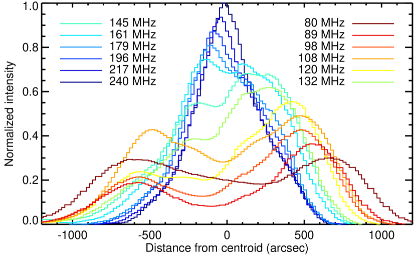
Figure 9.— Image slit intensities for each of the 12 MWA channels along the elongation axes of the individual burst source regions, illustrating the splitting of the source region from high to low frequencies. These data correspond to a period when the source regions are maximally extended at 05:17:26.6 UT. Each curve is normalized and multiplied by a scaling factor from 0.3–1.0 for clarity.

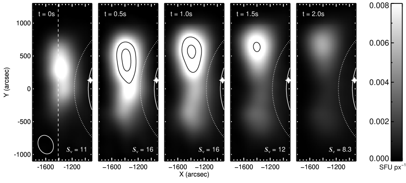
Figure 10.— Source splitting motion at 108 MHz, beginning at T. The dashed line in the left panel denotes the slit used in Fig. 11. The two solid black contours in the source region are at 0.010 and 0.015 SFU px^-1. Additional annotations are as in Fig. 4.

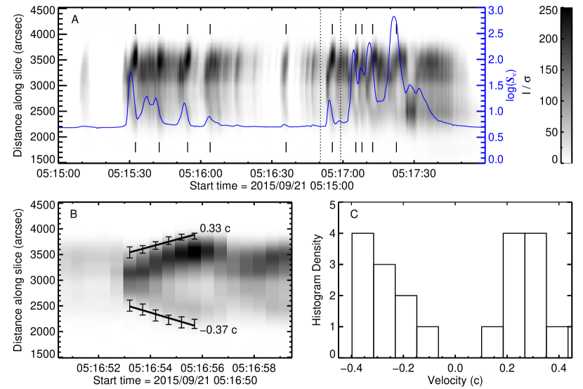
Figure 11.— An overview of the source splitting kinematics at 108 MHz. Panel A shows a distance-time plot using the slit shown in Fig. 10 along with a light curve of the total flux density in blue. Dotted vertical lines demarcate the zoomed-in section in Panel Bertical ticks mark the 10 speed measurement periods whose results are collected in Panel C. Error bars in Panel B reflect the range of leading-edge estimates, obtained by thresholding the two components by 15–25% of their maximum $I\cdot{}\sigma{}^{-1}$ values.

3.3. Type III Source Structure & Motion

The type III bursts begin around 05:15:30 UT during the early rise phase of the X-ray flare and continue at intervals through the decay phase. The two main bursts distinguishable in the Learmonth and Culgoora spectrographs are approximately coincident with the hard X-ray peak around 05:17 UT (Figure 1). The more sensitive and temporally-resolved MWA observations reveal these events to have a complicated dynamic spectrum structure that we interpret as the overlapping signatures of multiple electron injections in a brief period (Figure 2).

Throughout all of the bursts, a consistent pattern emerges in both the spatial structure of the source regions as a function of frequency and in their motions at particular frequencies. At higher frequencies, the type III source region is dominated by one spatial component with a much fainter component immediately to the north. Moving to lower frequencies and correspondingly larger heights, the two components separate along a direction tangent to the limb, reaching a peak-to-peak separation of 1200$\arcsec$ (1.25 R_⊙) at 80 MHz. This structure is clear from the burst images in Figure 4 and is illustrated in further detail by Figure 9.

Figure 9 plots intensities extracted from image slits along the directions for which the emission is maximally extended. Slit orientations are determined by fitting ellipses to the overall source region in each channel after thresholding the images above 20% of their peak intensities. Distances refer to that from the ellipse centers along their major axes, with values increasing from south to north. For clarity, the intensities are normalized and then multiplied by arbitrary scaling factors between 0.3 and 1.0 from low to high frequencies. At least two Gaussian components are required to fit the curves at all frequencies, though the northern component is manifested only as a non-Gaussian shoulder on the dominant component at high frequencies. At some frequencies (e.g. 108 MHz), there are also additional weaker peaks between the two main components. Interpretation of the varying burst morphology as a function of frequency is given in §4.

The type III source region components also spatially diverge as a function of time within single-channel observations below $\sim$132 MHz. At higher frequencies, for which there are one or two closely-spaced components, the source regions instead become increasingly elongated with time. The direction of this motion is essentially the same as that of the frequency-dependent splitting, and the timescales for it are quite short, on the order of $\sim$2 s. This motion is repeated many times throughout the event, with each burst and corresponding “split” interpreted as a distinct particle acceleration episode. An example image set is shown in Figure 10 for 108 MHz, the frequency that exhibits the highest intensities relative to the background.

To quantify this behavior, we employ distance-time maps to track movement along a particular slice through the images. The emission along the slit shown in the left panel of Figure 10 is extracted from each observation and stacked against those from adjacent images, such that each vertical column of Figures 11a and  11b represents the slit intensity at a given time. Slopes in the “slit image” correspond to plane-of-sky velocity components in the slit direction. Figure 11a shows the result of this analysis for the bursts during the first MWA observation period, lasting nearly 3 minutes after 05:15 UT. Intensities have been divided by the time-dependent noise level, defined as the standard deviation of values within a 5-pixel-wide border around the edge of each image (equivalent in area to a 75$\times$75 px, or 25$\times$25 arcmin, box). Because the noise level is roughly proportional to the total intensity, which varies by 2–3 orders of magnitude, this operation flattens the dynamic range of the distance-time map and provides for the uniform thresholding scheme described next.

The leading edges of the two source regions (north and south) are defined and tracked independently by thresholding the slit image above a percentage of the peak signal-to-noise ratio (SNR) for each component. Measurements are made for each burst using 11 integer thresholds between between 15 and 25% of the peak SNR. rror bars in Figure 11b represent the resulting range of leading edge locations, and corresponding speed uncertainties are on the order of 15%. An SNR percentage is used instead of a single set of values for both sources because it expands the range of reasonable thresholds, better representing the measurement uncertainties compared to a more restrictive range that would be appropriate for both sources.

Vertical ticks in Figure 11a mark the 10 bursts for which speed measurements were made at 108 MHz, and a histogram of the results is plotted in Figure 11c. The time periods were chosen for particularly distinct source separation for which both components could be tracked. It is clear from Figure 11a that the splitting motion occurs over a few additional periods for which measurements were precluded by confusion with adjacent events, faintness, or duration. We find speeds ranging between 0.11 and 0.40 c, averaging 0.26 c for the northern component and 0.28 c for the southern. The southern component is consistently faster for the 6 measurements before 05:16:55 UT and consistently slower after, but these differences are not statistically significant. These values cannot be straightforwardly interpreted as the exciter or electron beam speed ecause that would require electrons traveling along flux tubes parallel to the limb in a manner inconsistent with the inferred magnetic field configuration (§3.4). In §4, we will argue that this motion is a projected time-of-flight effect such that the splitting speeds here exceed the beam speed by a factor of $\lesssim$ 1.2.

he burst location at different frequencies as a function of time. We do this in Figure 12, which shows a distance-time plot similar to Figure 11. Instead of the emission along a particular slit, each column of Figure 12 corresponds to the total image intensity binned down to a single row. Pixels with the same horizontal X coordinate are averaged, hese veraged curves are stacked vertically against each other to show movement in the X direction. ince our source regions are distributed on either side of the equator, this roughly corresponds to radial motion

To we track the center position at the onset of the burst for each channel, which we define as 5$\times$ the background intensity. Center positions are determined by fitting a Gaussian to the relevant time column. e choose to examine the earliest burst period, occurring from 05:15:29–05:15:35 UT at frequencies below $\sim$132 MHz, because that event can be easily followed from high to low frequencies, whereas the more intense bursts later appear to everal overlapping events. Fitting a line to the resulting spatiotemporal positions in Figure 12, we find a speed of 0.17 c. This result reflects the average outward motion of the entire source, which can be taken as a lower limit to the exciter speed.

In comparison, the 108 MHz splitting speed for the same period averages to 0.28 c for both components, which as we will discuss in §4, hus we have a range of 0.17–0.28 c for the burst from 05:15:29–05:15:35 UT. Note that although the speeds from Figures 11 and 12 are measured in orthogonal directions, we cannot combine them in a quadrature sum as though they were components of one velocity vector. As we will explain next, this is because we interpret the source behavior in terms of several adjacent electron beams, each with a slightly different trajectory than the next, as opposed to one coherent system.

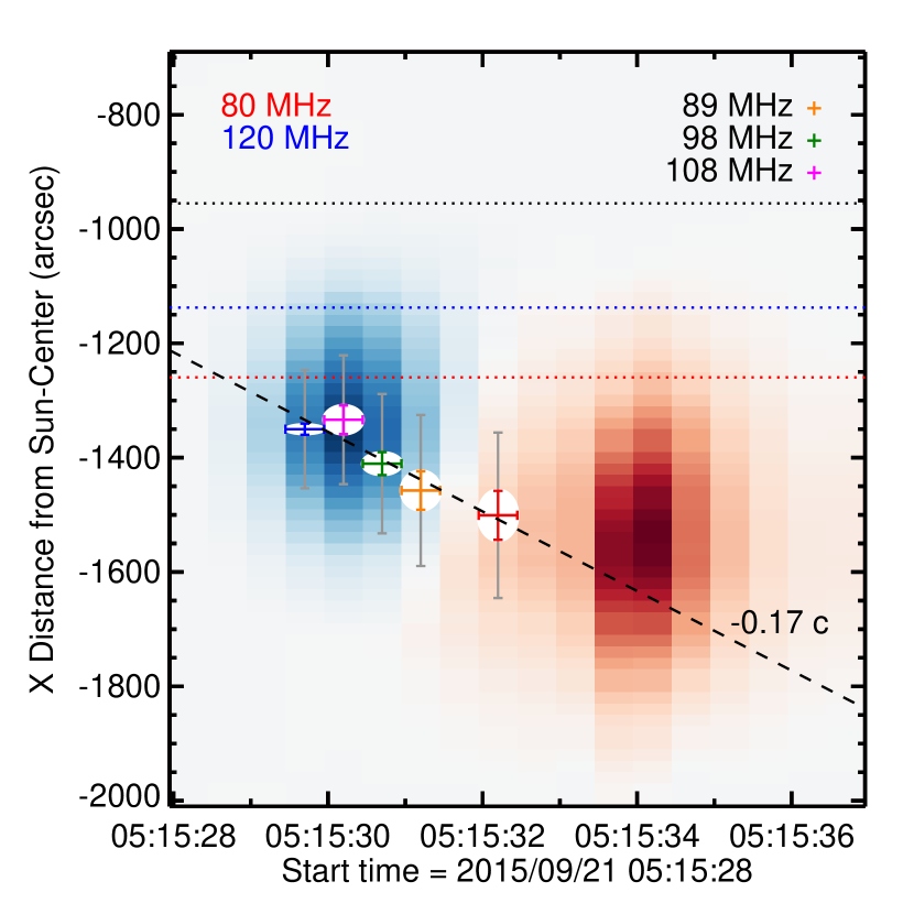
Figure 12.— Distance-time plot for burst emission from 05:15:28 to 05:15:37 UT. Red (80 MHz) and blue (120 MHz) images represent background-subtracted intensities averaged in the solar-Y direction, such that the slope reflects overall source motion in the solar-X direction. Crosshairs denote the burst onset times and centroid positions for each given frequency, where the onset is defined as exceeding 5$\times$ the background, Error bars correspond to the 0.5s time resolution (horizontal), the 3$\sigma{}$ variation in position over the burst period (vertical), and the minor synthesized beam axes (vertical, grey). Dotted horizontal lines represent the optical limb (black) and the Newkirk-model limbs at 80 (red) and 120 (blue) MHz.

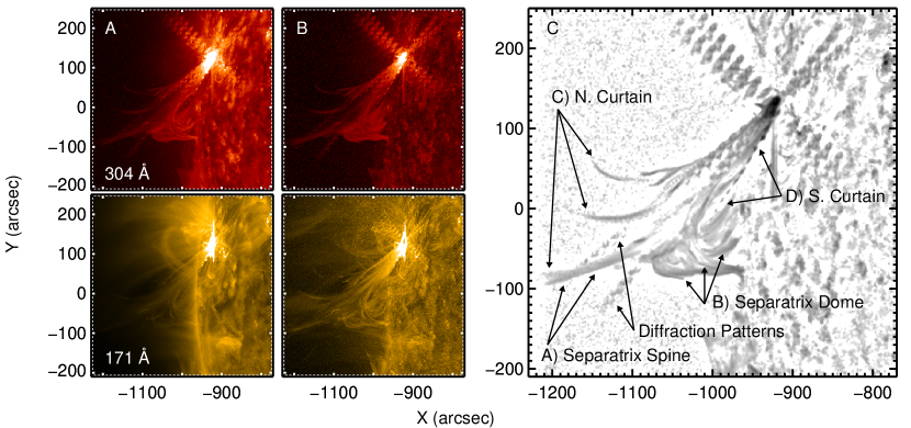
Figure 13.— A) Maximum value persistence maps for AIA 304 (top) and 171 Å (bottom). B) Column A subtracted by median backgrounds. C) Annotated 304-Å, background-subtracted persistence map, further processed to accentuate features. See §3.4 for processing details and Fig. 15 for a corresponding cartoon model. A corresponding movie is available in the online material.

3.4. Magnetic Field Configuration

Electron beams responsible for type III bursts propagate along magnetic field lines from the reconnection site, and therefore understanding the magnetic field configuration is critical to understanding the radio source region behavior and vice versa. Active region 12420, where the flare occurs, had just rotated into visibility on the east limb at the time of this event. EUV jets that immediately follow the radio bursts after the flare peak reveal a complex magnetic field configuration that connects AR 12420 to a small, diffuse dipole to the south near the equator. The southern region was just behind the limb during the flare, and based on its evolution in HMI magnetograms over the following days, appears to have been a decaying active region near the end of its evolution.

Unfortunately, this system is a poor candidate for local magnetic field modeling because of its partial visibility and position on the limb, where magnetogram observations are hampered by projection effects. The east limb position prevents us from using data from a few days prior, which is a possibility for west-limb events, and the decay of the southern dipole, along with the emergence of a neighboring region, dissuades us from attempting any dedicated modeling using data from subsequent days. Fortunately, the EUV jets trace out the field structure to an extent that we believe is sufficient to understand our observations. Previous studies have also demonstrated that type III electron beams are aligned with corresponding EUV and X-ray jets (e.g. Chen et al. 2013a), meaning that field lines traced out by the jets are preferentially those traversed by the accelerated electrons.

We employ maximum-value persistence mapping to compile the separate EUV jet paths into one image. This style of persistence map refers simply to plotting the largest value a given pixel achieves over some period (Thompson & Young, 2016). Our maps cover from 05:18 to 05:39 UT, which corresponds to when the EUV jets begin around the peak flare time until they reach their full spatial extent visible to AIA around 20 minutes later. To further enhance the contrast, we subtract the persistence maps by a median-value background over the same period (i.e. $I_{\rm max}-I_{\rm med}$). Figures 13a and  13b show maximum-value and background-subtracted persistence maps for both the 304 and 171 Å channels, which are most sensitive to the jet material. Figure 13c shows a version of the 304 Å map that has been Fourier filtered to suppress noise using a Hann window and then sharpened using an unsharp mask to accentuate the structure.

The EUV jets trace out a toplogy, not apparent just prior to the flare, where the field connectivity changes rapidly. Such regions are generally known as quasi-separatrix layers (QSLs; Priest & Démoulin 1995; Demoulin et al. 1996), which are 3D generalizations of 2D separatrices that separate magnetic field connectivity domains. The key distinction is that the field linkage across a QSL is not discontinuous as in a true separatrix but instead changes drastically over a relatively small spatial scale, which can be quantified by the squashing factor $Q$ (Titov, 2007). QSLs are important generally because they are preferred sites for the development of current sheets and ultimately magnetic reconnection (Aulanier et al., 2005). They are an essential part of 3D generalizations of the standard flare model (Janvier et al., 2013), and modeling their evolution can reproduce a number of observed flare features (e.g. Savcheva et al. 2015, 2016; Janvier et al. 2016). Here, we are less concerned with the dynamics of the flare site itself and focus instead on the neighboring region revealed by the EUV jets, which exhibits a topology associated with coronal null points.

We first note that our observed structure is similar in several ways to that modeled by Masson et al. (2012) and observed by Masson et al. (2014). The essential components are firstly the closed fan surface, or separatrix dome, and its single spine field line that is rooted in the photosphere and crosses the dome through the null point (Lau & Finn, 1990; Pontin et al., 2013). Open and closed flux domains are bounded above and below a separatrix dome, which can form when a dipole emerges into a preexisting open field region (e.g. Török et al. 2009). Above the dome and diverging around the null point is a vertical fan surface, or separatrix curtain, comprised of field lines extending higher into the corona, with those closest to the separatrix spine likely being open to interplanetary space. Potential field source surface (PFSS; Schrijver & De Rosa 2003) extrapolations (not shown) do predict open field in this region but do not reproduce other topological features, which is to be expected given the modeling challenges described above. Some openness to interplanetary space must also have been present to facilitate the corresponding interplanetary burst observed by Wind and shown in Figure 2.

The separatrix dome, spine, and part of the curtain are clearly delineated by the EUV jets and are labeled in Figure 13c. Note that some of the features, namely the closed field line associated with the southern portion of the separatrix curtain, are somewhat difficult to follow in Figure 13c but can be clearly distinguished in the corresponding movie available in the online material. In the following section, we will discuss how both types of source splitting described in §3.3 are facilitated by this topology.

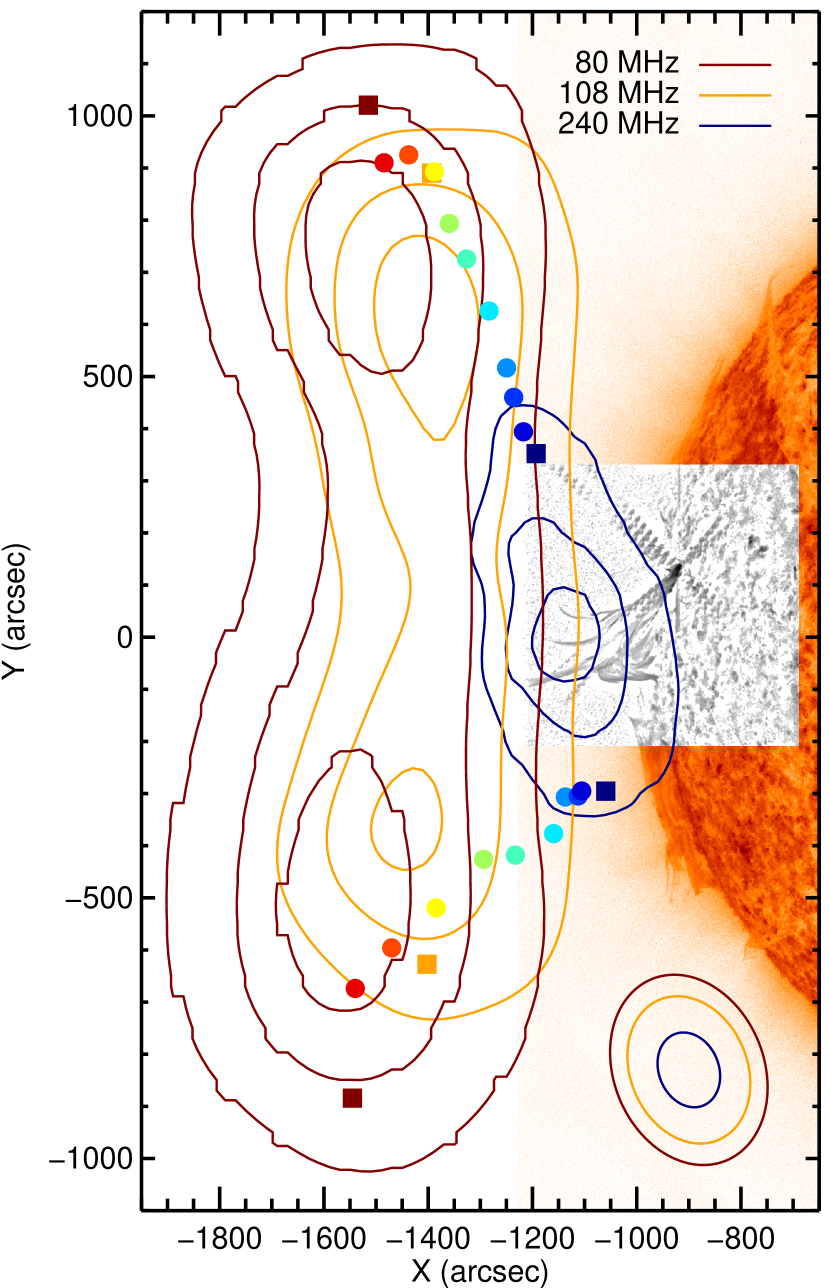
Figure 14.— MWA type III burst contours overlaid on a 304 Å SDO image. The greyscale inset is the persistence map from Fig. 13c. Pairs of colored dots represent the angular extent of the MWA source region in all 12 channels, with the squares from left to right corresponding to the 80 MHz), 108 MHz), and lue (240 MHz) contours, respectively. he MWA data are from a period when the source regions are maximally extended around 05:17:26.6 UT, and the SDO image combines data from the EUV jet period that follows (see §3.4).

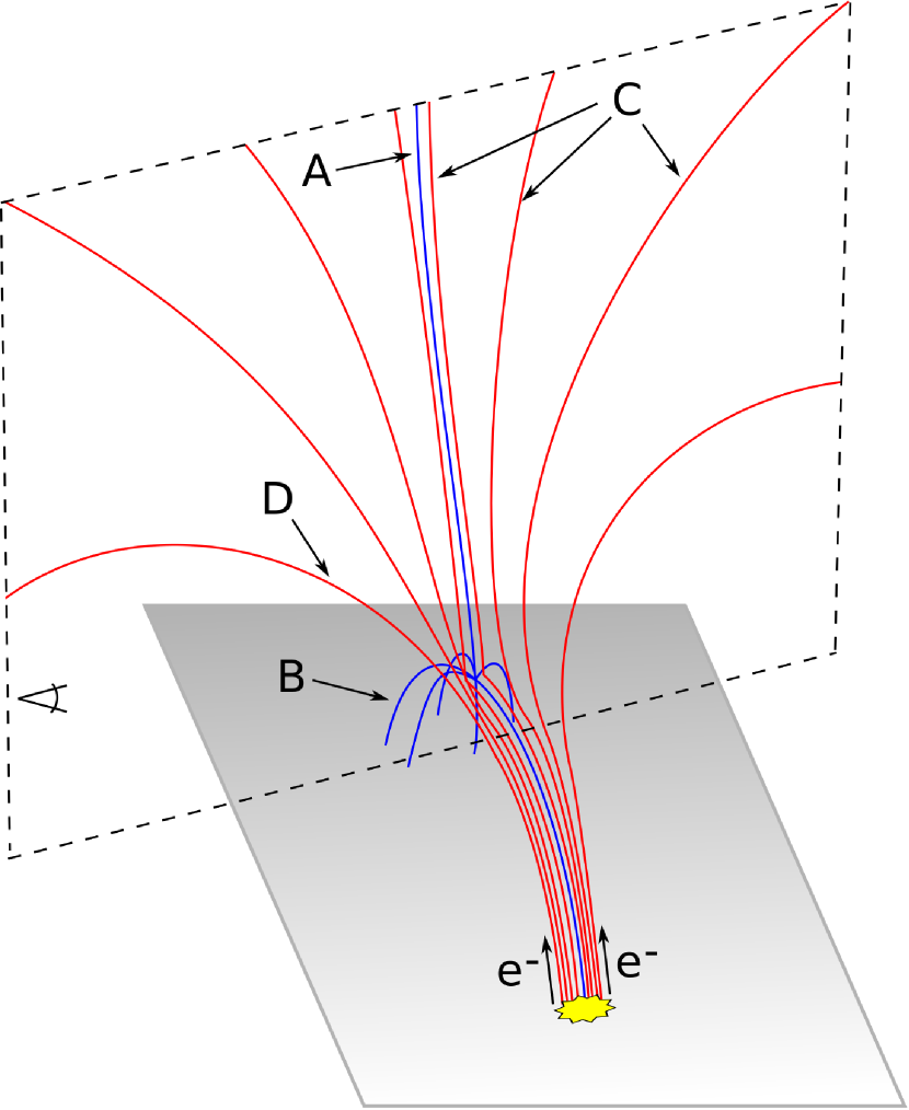
Figure 15.— Cartoon interpretation of the magnetic field configuration inferred from the EUV jet morphology and radio source regions (Fig. 14). The yellow region denotes the flare site, which is connected to a neighboring region with open and closed QSLs. Red field lines form a separatrix curtain, with the field closest to the center being open to interplanetary space. The blue field lines represent the closed separatrix dome, with a single spine field line that crosses the dome through a magnetic null point. Electrons travel along the diverging field lines of the separatrix curtain to produce the radio source structure and motion. Capital letters correspond to features apparent in the EUV observations (Fig. 13).

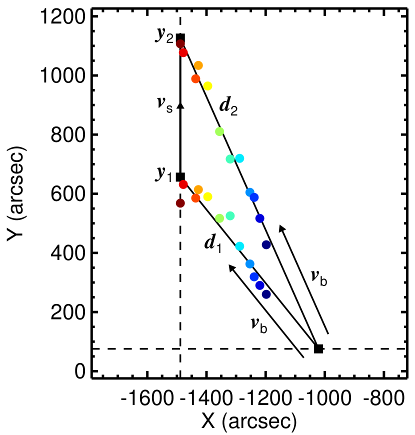
Figure 16.— Model schematic for the source splitting motion (Eqn. 1). Pairs of colored dots represent the average minimum and maximum vertical extents during each splitting episode; colors indicate frequency as in Figs. 9 & 14. The flux tubes along which the type III beams travel are approximated by the solid fit lines, which intersect near the observed null point (Fig. 13). Electrons take slightly longer to reach $y_{2}$ compared to $y_{1}$, which produces the apparent vertical motion with velocity $v_{\rm s}$. In reality, there would be a number of adjacent curved flux tubes between and below the two lines with nearby, but not identical, origins.

4. Discussion

When we overplot contours of the type III burst emission on the persistence map of the EUV jets (Figure 14), we see that the 240 MHz emission is concentrated just above the separatrix dome. As we described in §3.3, the burst emission splits with decreasing frequency (increasing height) into two increasingly-separated components. Figure 14 shows that the two components are distributed on either side of the separatrix spine. This implies a two-sided separatrix curtain with open field lines on either side of the spine, of which only the northern set are readily apparent in the EUV images. Given the position of the southern radio source and the closed field line that appears to form part of the southern curtain (D) in Figure 13, the southern half of the separatrix curtain seems to be oriented largely along the line of sight, which may explain why it is difficult to discern from the EUV jet structure. This two-sided separatrix curtain differs from the one-sided structure of Masson et al. (2012, 2014), but a number of other studies consider somewhat similar topologies (Maclean et al., 2009; van Driel-Gesztelyi et al., 2012; Titov et al., 2012; Craig & Pontin, 2014; Pontin & Wyper, 2015).

In Figure 15, we sketch a 3D field configuration based on the aforementioned modeling studies that fits the EUV structure and extrapolates from there to satisfy the connectivity required by the radio source distribution. This cartoon can parsimoniously explain both the spatial splitting of the source from high to low frequencies and the source motion observed for individual frequency channels. Type III bursts emit at the local plasma frequency or its second harmonic ($f\approx f_{p}$ or $2f_{p}$), which is proportional to the square of the ambient electron density. Thus, emission at a particular frequency can be associated with a particular height corresponding to the requisite background density. In our interpretation, electrons travel simultaneously along each of the red field lines in Figure 15. The electron beams diverge on either side of the separatrix curtain, such that the beams are nearest to each other at lower heights (higher frequencies) and furthest apart at larger heights (lower frequencies). This produces the spatial source splitting and the dramatic increase of the overall angular extent toward lower frequencies, which is illustrated by the pairs of colored dots in Figure 14. The source motions illustrated by Figures 10 and 11 can then be accounted for as a projected time-of-flight effect. Electrons moving along the increasingly curved outer field lines take slightly longer to reach the same height, producing emission at adjacent positions along the separatrix curtain at slightly later times for a given frequency. hus, the splitting speeds measured in §3.3 are not the exciter or electron beam speeds. They are instead somewhat faster, depending on the difference in travel time to a given height along adjacent flux tubes. Adopting the geometry in Figure 16, the expression for this is:

$$v_{\rm s}=\frac{y_{2}-y_{1}}{d_{2}-d_{1}}v_{\rm b}~{},$$ (1)

where $v_{\rm s}$ is the apparent source splitting speed, $v_{\rm b}$ is the electron beam speed, $y_{1,2}$ are solar Y coordinates, and $d_{1,2}$ are the distances traveled along the field lines to reach $y_{1,2}$.

To estimate these parameters, we determine the average minimum and maximum vertical extents of the source regions for each frequency by fitting ellipses to every burst image, he X coordinates of the northern vertices are averaged, and the Y coordinates one standard deviation above and below the mean are averaged separately to obtain the pairs of colored dots in Figure 16. If we approximate the field lines as linear fits to these points, which intersect close to the observed null point (Figure 13), then the speed of the source motion is 1.16$\times$ the beam speed. Taking each of the lower-frequency points individually, we find factors ranging from 1.14 at 120 MHz to 1.19 at 80 MHz. Slightly larger factors are found for lower frequencies because of the larger separations between $y_{1}$ and $y_{2}$ compared to the fit projection, which may be due to the field lines curving out with height.

Using the 1.16 factor, orresponds to an average f 0.2 c. This value is consistent with and provides independent confirmation of beam speeds estimated from frequency drift rates, which is possible if one assumes a density model. Modest fractions of light speed are typical in the corona (e.g. Alvarez & Haddock 1973; Aschwanden et al. 1995; Meléndez et al. 1999; Kishore et al. 2017), but some studies have found values in excess of 0.5 c (Poquerusse, 1994; Carley et al., 2016) and even superluminal velocities given the right projection geometry (Klassen et al., 2003). We also note that similar observations could be used to robe the coronal density structure ecause our imaging capability allows us to estimate ithout assuming a density model using time- and frequency-varying source positions in the manner illustrated by Figure 12. This particular event is not ideal for that analysis because of the complicated source structure, but a followup study is planned for a small ensemble of events that exhibit simple source structures without the type of motion described here. A few other connections to the literature should be mentioned with respect to the observed radio structure and inferred field configuration. First, we see from Figure 6 and in the movie associated with Figures 3 and 4 that the source region of the bursts at 240 MHz is consistently enhanced and exhibits low-level burst activity outside of the intense burst periods. Figure 14 demonstrates that this emission is concentrated just above the separatrix dome and associated null point. These structures are interface regions between closed and open magnetic flux, where interchange reconnection may be ongoing (e.g. Masson et al. 2012, 2014). Such regions have previously been associated with radio enhancements and noise storms (Wen et al., 2007; Del Zanna et al., 2011; Régnier, 2013).

A few Nançay Radioheliograph (NRH) observations exhibit characteristics reminiscent of those described here. For instance, Paesold et al. (2001) conclude that the spatial separation of temporally adjacent type III events predominantly resulted from different field line trajectories followed by the electron beams. Reid et al. (2014) show a number of elliptically extended type III source regions that are represented as enveloping the diverging paths of electrons accelerated from the same site. Our observations that overlap in frequency with the NRH range ($\geq$150 MHz) are similarly extended to a larger degree before separating into two primary components at lower frequencies. Carley et al. (2016) describe a “radio arc” in their lowest-frequency images that is strikingly similar to our observations (e.g. Figure 14) but is suggested instead to trace the boundary of an erupting coronal mass ejection.

ote that the complicated structure exhibited by the MWA dynamic spectrum (Figures 2 & 8) may indicate the presence of other burst types. Classic type III emission drifts from high to low frequencies as electron beams propagate outward into interplanetary space. If confined to closed field lines, the same beams may produce type U or J bursts for which the frequency drift rate switches signs as electrons crest the closed loops and propagate back toward the Sun (Maxwell & Swarup, 1958; Aurass & Klein, 1997; Reid & Kontar, 2017). We see hints of this in our dynamic spectrum at $\sim$196 MHz around 05:17:40 UT (Figure 2), but it is difficult to interpret because of the MWA’s sparse frequency coverage. Given that our interpretation of the magnetic field configuration (Figure 15) includes closed field lines on either side of the separatrix curtain, such features in the dynamic spectrum would not be surprising. Our splitting motion could also be due partially to beams traveling largely tangent to the limb along such closed field lines, while adjacent beams make it to larger heights along field lines closer to the separatrix spine, but evidence for downward propagation is lacking in the images.

5. Conclusion

We have presented the first time series imaging study of MWA solar data. Our observations reveal complex type III burst source regions that exhibit previously unreported dynamics. We identify two types of source region splitting, one being a frequency-dependent structure and the other being source motion within individual frequency channels. For the former, the source regions splits from one dominant component at our highest frequency (240 MHz) into two increasingly separated sources with decreasing frequency down to 80 MHz. This corresponds to a straightforward splitting of the source region as a function of height, with larger separations at larger heights.

With high time resolution imaging, we observe a splitting motion within the source regions at individual frequencies, particularly in the lower channels ($\lesssim$ 132 MHz), that is tangent to the limb in essentially the same direction as the source splitting from high to low frequencies. This motion is short-lived ($\sim$2 s), fast (0.1–0.4 c), and repetitive, occurring multiple times over a period of 7 min before, during, and after the X-ray flare peak. We interpret the repetitive nature as multiple electron beam injections that produce distinct radio bursts with overlapping signatures in the dynamic spectrum, which is consistent with there being several distinct EUV jet episodes that immediately follow the radio bursts.

The EUV jets, which are assumed to have very similar trajectories to the type III electron beams, trace out a region where the magnetic field connectivity rapidly diverges over a small spatial scale. These types of configurations are broadly referred to as QSLs, and we argue that this field structure facilitates the radio source region splitting. Several common topological features associated with coronal null points are identifiable in persistence maps of the EUV outflows, including a separatrix dome, spine, and curtain. Electrons are accelerated simultaneously along adjacent field lines that connect the flare site to an open QSL, where their paths diverge to produce the source region splitting. At 240 MHz, the burst emission is concentrated just above the separatrix dome, a region that is consistently enhanced outside of burst periods. Moving to larger heights (lower frequencies), the source regions split on either side of the separatrix spine. he northern radio component is consistent with field lines apparent from the EUV observations, but the southern component implies a two-sided separatrix curtain that is not obvious from the EUV observations. Thus, the radio imaging provides additional constraints on the magnetic field connectivity.

The magnetic field configuration also offers a straightforward explanation for the radio source motion via a projected time-of-flight effect, whereby electrons moving along slightly longer outer field lines take slightly longer to excite emission at adjacent positions of roughly the same radial height. Given this interpretation, the speed of the source region is a factor of $\lesssim$ 1.2$\times$ greater than the electron beam speed. We estimate an average beam speed of 0.2 c, which is an independent confirmation of speeds estimated from frequency drift rates. We note that the same characteristics are observed in another type III burst from the same region three hours earlier. This implies that the field topology is stable at least on that timescale and strengthens our conclusion that the radio dynamics are caused by interaction with a preexisting magnetic field structure, as opposed to peculiarities of the flare process itself.

Lastly, we motivate future studies of MWA solar observations. A survey of type III bursts is underway. From preliminary results, we note that the dual-component splitting behavior described here is uncommon. However, analogous source region motion in one direction is common and could be explained in the same manner if coupled with a consistent picture of the particular field configurations. Similar events that occur near disk center or on the opposite (west) limb could be combined with magnetic field modeling to develop a more detailed topological understanding. The coronal density structure can also be probed by examining events with less complicated source structures. Finally, we showed a coronal hole that gradually transitions from dark to bright from high to low frequencies, turning over around 120 MHz. This adds a transition point to the small body of literature reporting coronal holes in emission at low frequencies, an effect that is not well-explained and could be addressed with additional MWA observations.

References

- Alissandrakis (1994) Alissandrakis, C. E. 1994, Advances in Space Research, 14
- Alissandrakis et al. (2015) Alissandrakis, C. E., Nindos, A., Patsourakos, S., Kontogeorgos, A., & Tsitsipis, P. 2015, A&A, 582, A52
- Alvarez & Haddock (1973) Alvarez, H., & Haddock, F. T. 1973, Sol. Phys., 29, 197
- Arzner & Benz (2005) Arzner, K., & Benz, A. O. 2005, Sol. Phys., 231, 117
- Aschwanden et al. (1995) Aschwanden, M. J., Benz, A. O., Dennis, B. R., & Schwartz, R. A. 1995, ApJ, 455, 347
- Aubier et al. (1971) Aubier, M., Leblanc, Y., & Boischot, A. 1971, A&A, 12, 435
- Aulanier et al. (2005) Aulanier, G., Pariat, E., & Démoulin, P. 2005, A&A, 444, 961
- Aurass & Klein (1997) Aurass, H., & Klein, K.-L. 1997, A&AS, 123
- Aurass et al. (1994) Aurass, H., Klein, K.-L., & Martens, P. C. H. 1994, Sol. Phys., 155, 203
- Bastian (1994) Bastian, T. S. 1994, ApJ, 426, 774
- Benz et al. (2007) Benz, A. O., Brajša, R., & Magdalenić, J. 2007, Sol. Phys., 240, 263
- Benz et al. (2005) Benz, A. O., Grigis, P. C., Csillaghy, A., & Saint-Hilaire, P. 2005, Sol. Phys., 226, 121
- Bougeret et al. (1995) Bougeret, J.-L., Kaiser, M. L., Kellogg, P. J., et al. 1995, Space Sci. Rev., 71, 231
- Bowman et al. (2013) Bowman, J. D., Cairns, I., Kaplan, D. L., et al. 2013, PASA, 30, e031
- Briggs (1995) Briggs, D. S. 1995, in Bulletin of the American Astronomical Society, Vol. 27, American Astronomical Society Meeting Abstracts, 1444
- Brown & Melrose (1977) Brown, J. C., & Melrose, D. B. 1977, Sol. Phys., 52, 117
- Cairns et al. (2017) Cairns, I. H., Lobzin, V. V., Donea, A., et al. 2017, Nature Scientific Reports, submitted
- Carley et al. (2016) Carley, E. P., Vilmer, N., & Gallagher, P. T. 2016, ApJ, 833, 87
- Chen et al. (2013a) Chen, B., Bastian, T. S., White, S. M., et al. 2013a, ApJ, 763, L21
- Chen et al. (2013b) Chen, N., Ip, W.-H., & Innes, D. 2013b, ApJ, 769, 96
- Craig & Pontin (2014) Craig, I. J. D., & Pontin, D. I. 2014, ApJ, 788, 177
- Del Zanna et al. (2011) Del Zanna, G., Aulanier, G., Klein, K.-L., & Török, T. 2011, A&A, 526, A137
- Demoulin et al. (1996) Demoulin, P., Henoux, J. C., Priest, E. R., & Mandrini, C. H. 1996, A&A, 308, 643
- Downs et al. (2012) Downs, C., Roussev, I. I., van der Holst, B., Lugaz, N., & Sokolov, I. V. 2012, ApJ, 750, 134
- Dulk et al. (2001) Dulk, G. A., Erickson, W. C., Manning, R., & Bougeret, J.-L. 2001, A&A, 365, 294
- Dulk & Sheridan (1974) Dulk, G. A., & Sheridan, K. V. 1974, Sol. Phys., 36, 191
- Dulk et al. (1984) Dulk, G. A., Steinberg, J. L., & Hoang, S. 1984, A&A, 141, 30
- Freeland & Handy (1998) Freeland, S. L., & Handy, B. N. 1998, Sol. Phys., 182, 497
- Gibson et al. (2016) Gibson, S., Kucera, T., White, S., et al. 2016, Frontiers in Astronomy and Space Sciences, 3, 8
- Ginzburg & Zhelezniakov (1958) Ginzburg, V. L., & Zhelezniakov, V. V. 1958, Soviet Ast., 2, 653
- Guidice et al. (1981) Guidice, D. A., Cliver, E. W., Barron, W. R., & Kahler, S. 1981, in BAAS, Vol. 13, Bulletin of the American Astronomical Society, 553
- Hill et al. (2009) Hill, F., Martens, P., Yoshimura, K., et al. 2009, Earth Moon and Planets, 104, 315
- Hoang & Steinberg (1977) Hoang, S., & Steinberg, J. L. 1977, A&A, 58, 287
- Hong et al. (2017) Hong, J., Jiang, Y., Yang, J., Li, H., & Xu, Z. 2017, ApJ, 835, 35
- Hurley-Walker et al. (2014) Hurley-Walker, N., Morgan, J., Wayth, R. B., et al. 2014, PASA, 31, e045
- Hurley-Walker et al. (2017) Hurley-Walker, N., Callingham, J. R., Hancock, P. J., et al. 2017, MNRAS, 464, 1146
- Ingale et al. (2015) Ingale, M., Subramanian, P., & Cairns, I. 2015, MNRAS, 447, 3486
- Innes et al. (2016) Innes, D. E., Bučík, R., Guo, L.-J., & Nitta, N. 2016, Astronomische Nachrichten, 337, 1024
- Janvier et al. (2013) Janvier, M., Aulanier, G., Pariat, E., & Démoulin, P. 2013, A&A, 555, A77
- Janvier et al. (2016) Janvier, M., Savcheva, A., Pariat, E., et al. 2016, A&A, 591, A141
- Kennewell & Steward (2003) Kennewell, J., & Steward, G. 2003, Solar Radio Spectrograph [SRS] Data Viewer, Tech. rep., Sydney, IPS Radio and Space Serv.
- Kerdraon & Delouis (1997) Kerdraon, A., & Delouis, J.-M. 1997, in Lecture Notes in Physics, Berlin Springer Verlag, Vol. 483, Coronal Physics from Radio and Space Observations, ed. G. Trottet, 192
- Kishore et al. (2017) Kishore, P., Kathiravan, C., Ramesh, R., & Ebenezer, E. 2017, Journal of Astrophysics and Astronomy, 38, #24
- Klassen et al. (2003) Klassen, A., Karlický, M., & Mann, G. 2003, A&A, 410, 307
- Krucker et al. (2007) Krucker, S., Kontar, E. P., Christe, S., & Lin, R. P. 2007, ApJ, 663, L109
- Kundu et al. (1983) Kundu, M. R., Erickson, W. C., Gergely, T. E., Mahoney, M. J., & Turner, P. J. 1983, Sol. Phys., 83, 385
- Kundu et al. (1995) Kundu, M. R., Raulin, J. P., Nitta, N., et al. 1995, ApJ, 447, L135
- Lantos (1999) Lantos, P. 1999, in Proceedings of the Nobeyama Symposium, ed. T. S. Bastian, N. Gopalswamy, & K. Shibasaki, Vol. 479, 11
- Lantos et al. (1987) Lantos, P., Alissandrakis, C. E., Gergely, T., & Kundu, M. R. 1987, Sol. Phys., 112, 325
- Lau & Finn (1990) Lau, Y.-T., & Finn, J. M. 1990, ApJ, 350, 672
- Lemen et al. (2012) Lemen, J. R., Title, A. M., Akin, D. J., et al. 2012, Sol. Phys., 275, 17
- Li et al. (2011a) Li, B., Cairns, I. H., & Robinson, P. A. 2011a, ApJ, 730, 21
- Li et al. (2011b) —. 2011b, ApJ, 730, 20
- Li et al. (2012) —. 2012, Sol. Phys., 279, 173
- Lin et al. (2002) Lin, R. P., Dennis, B. R., Hurford, G. J., et al. 2002, Sol. Phys., 210, 3
- Lionello et al. (2009) Lionello, R., Linker, J. A., & Mikić, Z. 2009, ApJ, 690, 902
- Loi et al. (2014) Loi, S. T., Cairns, I. H., & Li, B. 2014, ApJ, 790, 67
- Lonsdale et al. (2009) Lonsdale, C. J., Cappallo, R. J., Morales, M. F., et al. 2009, IEEE Proceedings, 97, 1497
- Maclean et al. (2009) Maclean, R. C., Büchner, J., & Priest, E. R. 2009, A&A, 501, 321
- Masson et al. (2012) Masson, S., Aulanier, G., Pariat, E., & Klein, K.-L. 2012, Sol. Phys., 276, 199
- Masson et al. (2014) Masson, S., McCauley, P., Golub, L., Reeves, K. K., & DeLuca, E. E. 2014, ApJ, 787, 145
- Maxwell & Swarup (1958) Maxwell, A., & Swarup, G. 1958, Nature, 181, 36
- Meléndez et al. (1999) Meléndez, J. L., Sawant, H. S., Fernandes, F. C. R., & Benz, A. O. 1999, Sol. Phys., 187, 77
- Melrose (2009) Melrose, D. B. 2009, in IAU Symposium, Vol. 257, Universal Heliophysical Processes, ed. N. Gopalswamy & D. F. Webb, 305
- Mercier & Chambe (2012) Mercier, C., & Chambe, G. 2012, A&A, 540, A18
- Mikić et al. (1999) Mikić, Z., Linker, J. A., Schnack, D. D., Lionello, R., & Tarditi, A. 1999, Physics of Plasmas, 6, 2217
- Morosan et al. (2014) Morosan, D. E., Gallagher, P. T., Zucca, P., et al. 2014, A&A, 568, A67
- Mulay et al. (2016) Mulay, S. M., Tripathi, D., Del Zanna, G., & Mason, H. 2016, A&A, 589, A79
- Newkirk (1961) Newkirk, Jr., G. 1961, ApJ, 133, 983
- Oberoi et al. (2017) Oberoi, D., Sharma, R., & Rogers, A. E. E. 2017, Sol. Phys., 292, #75
- Oberoi et al. (2011) Oberoi, D., Matthews, L. D., Cairns, I. H., et al. 2011, ApJ, 728, L27
- Oberoi et al. (2014) Oberoi, D., Sharma, R., Bhatnagar, S., et al. 2014, ArXiv e-prints, arXiv:1403.6250 [astro-ph.IM]
- Offringa et al. (2012) Offringa, A. R., van de Gronde, J. J., & Roerdink, J. B. T. M. 2012, A&A, 539, A95
- Offringa et al. (2014) Offringa, A. R., McKinley, B., Hurley-Walker, N., et al. 2014, MNRAS, 444, 606
- Offringa et al. (2015) Offringa, A. R., Wayth, R. B., Hurley-Walker, N., et al. 2015, PASA, 32, e008
- Ord et al. (2015) Ord, S. M., Crosse, B., Emrich, D., et al. 2015, PASA, 32, e006
- Paesold et al. (2001) Paesold, G., Benz, A. O., Klein, K.-L., & Vilmer, N. 2001, A&A, 371, 333
- Pesnell et al. (2012) Pesnell, W. D., Thompson, B. J., & Chamberlin, P. C. 2012, Sol. Phys., 275, 3
- Pontin et al. (2013) Pontin, D. I., Priest, E. R., & Galsgaard, K. 2013, ApJ, 774, 154
- Pontin & Wyper (2015) Pontin, D. I., & Wyper, P. F. 2015, ApJ, 805, 39
- Poquerusse (1994) Poquerusse, M. 1994, A&A, 286, 611
- Prestage et al. (1994) Prestage, N. P., Luckhurst, R. G., Paterson, B. R., Bevins, C. S., & Yuile, C. G. 1994, Sol. Phys., 150, 393
- Priest & Démoulin (1995) Priest, E. R., & Démoulin, P. 1995, J. Geophys. Res., 100, 23443
- Ramesh et al. (2005) Ramesh, R., Narayanan, A. S., Kathiravan, C., Sastry, C. V., & Shankar, N. U. 2005, A&A, 431, 353
- Ramesh et al. (1998) Ramesh, R., Subramanian, K. R., Sundararajan, M. S., & Sastry, C. V. 1998, Sol. Phys., 181, 439
- Raulin et al. (1996) Raulin, J. P., Kundu, M. R., Nitta, N., & Raoult, A. 1996, ApJ, 472, 874
- Reeves & Golub (2011) Reeves, K. K., & Golub, L. 2011, ApJ, 727, L52
- Régnier (2013) Régnier, S. 2013, Sol. Phys., 288, 481
- Reid & Kontar (2017) Reid, H. A. S., & Kontar, E. P. 2017, ArXiv e-prints, arXiv:1706.07410 [astro-ph.SR]
- Reid & Ratcliffe (2014) Reid, H. A. S., & Ratcliffe, H. 2014, Research in Astronomy and Astrophysics, 14, 773
- Reid & Vilmer (2017) Reid, H. A. S., & Vilmer, N. 2017, A&A, 597, A77
- Reid et al. (2014) Reid, H. A. S., Vilmer, N., & Kontar, E. P. 2014, A&A, 567, A85
- Riddle (1974) Riddle, A. C. 1974, Sol. Phys., 36, 375
- Riley et al. (2011) Riley, P., Lionello, R., Linker, J. A., et al. 2011, Sol. Phys., 274, 361
- Robinson & Cairns (1994) Robinson, P. A., & Cairns, I. H. 1994, Sol. Phys., 154, 335
- Robinson & Cairns (2000) —. 2000, Washington DC American Geophysical Union Geophysical Monograph Series, 119, 37
- Saint-Hilaire et al. (2009) Saint-Hilaire, P., Krucker, S., Christe, S., & Lin, R. P. 2009, ApJ, 696, 941
- Saint-Hilaire et al. (2013) Saint-Hilaire, P., Vilmer, N., & Kerdraon, A. 2013, ApJ, 762, 60
- Savcheva et al. (2016) Savcheva, A., Pariat, E., McKillop, S., et al. 2016, ApJ, 817, 43
- Savcheva et al. (2015) —. 2015, ApJ, 810, 96
- Scherrer et al. (2012) Scherrer, P. H., Schou, J., Bush, R. I., et al. 2012, Sol. Phys., 275, 207
- Schrijver & De Rosa (2003) Schrijver, C. J., & De Rosa, M. L. 2003, Sol. Phys., 212, 165
- Schrijver et al. (2004) Schrijver, C. J., Sandman, A. W., Aschwanden, M. J., & De Rosa, M. L. 2004, ApJ, 615, 512
- Sheridan et al. (1972) Sheridan, K. V., Labrum, N. R., & Payten, W. J. 1972, Nature Physical Science, 238, 115
- Sheridan et al. (1983) Sheridan, K. V., Labrum, N. R., Payten, W. J., Nelson, G. J., & Hill, E. R. 1983, Sol. Phys., 83, 167
- Shibasaki et al. (2011) Shibasaki, K., Alissandrakis, C. E., & Pohjolainen, S. 2011, Sol. Phys., 273, 309
- Suresh et al. (2016) Suresh, A., Sharma, R., Oberoi, D., et al. 2016, ArXiv e-prints, arXiv:1612.01016 [astro-ph.SR]
- Sutinjo et al. (2015) Sutinjo, A., O’Sullivan, J., Lenc, E., et al. 2015, Radio Science, 50, 52
- Thejappa & MacDowall (2008) Thejappa, G., & MacDowall, R. J. 2008, ApJ, 676, 1338
- Thompson & Young (2016) Thompson, B. J., & Young, C. A. 2016, ApJ, 825, 27
- Thompson (2006) Thompson, W. T. 2006, A&A, 449, 791
- Tingay et al. (2013a) Tingay, S. J., Oberoi, D., Cairns, I., et al. 2013a, in Journal of Physics Conference Series, Vol. 440, Journal of Physics Conference Series, 012033
- Tingay et al. (2013b) Tingay, S. J., Goeke, R., Bowman, J. D., et al. 2013b, PASA, 30, e007
- Titov (2007) Titov, V. S. 2007, ApJ, 660, 863
- Titov et al. (2012) Titov, V. S., Mikic, Z., Török, T., Linker, J. A., & Panasenco, O. 2012, ApJ, 759, 70
- Török et al. (2009) Török, T., Aulanier, G., Schmieder, B., Reeves, K. K., & Golub, L. 2009, ApJ, 704, 485
- Trottet (2003) Trottet, G. 2003, Advances in Space Research, 32, 2403
- van Driel-Gesztelyi et al. (2012) van Driel-Gesztelyi, L., Culhane, J. L., Baker, D., et al. 2012, Sol. Phys., 281, 237
- van Haarlem et al. (2013) van Haarlem, M. P., Wise, M. W., Gunst, A. W., et al. 2013, A&A, 556, A2
- Weber (1978) Weber, R. R. 1978, Sol. Phys., 59, 377
- Wen et al. (2007) Wen, Y.-Y., Wang, J.-X., & Zhang, Y.-Z. 2007, CJAA, 7, 265
- White et al. (2011) White, S. M., Benz, A. O., Christe, S., et al. 2011, Space Sci. Rev., 159, 225
- Wild & McCready (1950) Wild, J. P., & McCready, L. L. 1950, Australian Journal of Scientific Research A Physical Sciences, 3, 387