Revisiting Higgs inflation in the context of collapse theories

Abstract

In this work we consider the Higgs inflation scenario, but in contrast with past works, the present analysis is done in the context of a spontaneous collapse theory for the quantum state of the inflaton field. In particular, we will rely on a previously studied adaptation of the Continuous Spontaneous Localization model for the treatment of inflationary cosmology. We will show that with the introduction of the dynamical collapse hypothesis, some of the most serious problems of the Higgs inflation proposal can be resolved in a natural way.

I Introduction

The inflationary paradigm has become an integral part of modern cosmology, in great part due to its empirically successful account of the primordial inhomogeneities that represent the origin of the cosmological structure. The most recent observational data of the CMB, as extracted from the PLANCK satellite observations, is consistent with the theoretical predictions made by many inflationary models Hinshaw et al. [2013], Ade [2014], including some of the single scalar field models Martin et al. [2014]. There is an outstanding problem regarding the still unobserved primordial tensor perturbations and we point the reader to Leon and Sudarsky [2013] for a re-assessment of the relevant expectations based on ideas related to the ones underlying the present work.

According to the inflationary paradigm, the explanation for the generation of primordial inhomogeneities that constitute the seeds of cosmic structure is the following: the perturbations start as quantum fluctuations associated with the vacuum state of the inflaton field, as the universe goes through an era of accelerated expansion. The physical wavelength associated with the perturbations is stretched out by the expansion, eventually reaching cosmological scales. At this point, quantum fluctuations are treated as describing the averages over an ensemble of inhomogeneous universes of their analogue classical quantities: classical density perturbations Mukhanov et al. [1992]. That last step, however does not seem to have a clear justification, as it has been noted in Perez et al. [2006] and pointed out in Weinberg’s book Weinberg [2008]. Ignoring that issue, the account concludes by indicating that these perturbations continue evolving into the cosmic structure responsible for galaxy formation, stars, planets and eventually life and human beings.

One of the least satisfactory features of the inflationary scenario is that it seems to require the incorporation of new fields or new degrees of freedom, which are not associated with other existing manifestations beyond those related to the inflationary process itself. It would be certainly a much more attractive scheme one in which inflation was tied instead to one of the known physical fields, and thus the idea that the role of the inflaton might be played by the Higgs was deemed very attractive. However the specific realization of such idea was faced with several problems related to the validity of the perturbation theory and the relative size of the radiative corrections Barbon and Espinosa [2009], Burgess et al. [2010], Hertzberg [2010].

On the other hand, and connected in a sense with Weinberg’s above mentioned concern, as it has been pointed out in various articles Sudarsky [2013], Canate et al. [2013] and extensively discussed Sudarsky [2011], there is a fundamental problem with the traditional point of view: there is simply no clear answer to the question of why, how and when did the homogeneity and isotropy of the universe break down. The point is that both the background, often described in a classical language, and the perturbations which are described in a quantum language, are both characterized by homogeneous and isotropic states. Regarding the quantum aspect to which the above mentioned fluctuations refer to, and that presumably give rise to the primordial inhomogeneities and anisotropies, the point is the following: the unitary evolution (process U Bell [1990]) of a quantum state follows the deterministic Schrödinger equation which preserves the symmetries of the initial state that are also symmetries of the action. By contrast, the process R (reduction) Bell [1990] associated with the measurement of an observable, which does force the system to collapse to one of the eigenstates of the measured observable in a indeterministic fashion, might break those symmetries. However, the R process can be called upon only when a measurement by an external observer/apparatus is involved. In other words, the problem of accounting for the breakdown of the symmetry resides in how we characterize the process that should be considered as a measurement. Without this characterization we cannot properly explain the emergence of the cosmological asymmetries when we have started with a completely homogeneous and isotropic state, such as the Bunch-Davies vacuum (an related states) in a FRW space-time, while the dynamics don’t break the symmetries. This is evidently a manifestation of the so-called measurement problem in quantum theory, which in fact becomes even more serious when we want to apply the quantum theory to the universe as a whole, simply because we can not even rely on the practical usage of identifying an observer and/or a measuring device. Simple “escape” strategies, like arguing that we as astronomers are acting as observers, would not do resolve the issues as, according to our understanding of cosmology, we ourselves must be consequence of the breakdown of symmetry that led to the generation of cosmological structure and thus cannot also be its cause. We will not dwell any further on the discussion of these issues here, and after acknowledging that the debate is not completely settled, we point the interested reader to the various works in which these issues are examined in detail and where the references to dissenting views are cited Sudarsky [2011], Okon and Sudarsky [2014].

The approach followed to address the issue, which was developed in several previous works Diez-Tejedor and Sudarsky [2012], is based on the incorporation into the inflationary paradigm of the hypothesis of self-induced collapse of the quantum state, an idea employed in modified versions of quantum theory designed precisely to address the measurement problem Bell [1990], Bassi and Ghirardi [2003].

In this paper we will show that the incorporation of the spontaneous collapse of quantum states into the theoretical framework offers, as a side benefit, a path to deal with the difficulties faced by the Higgs-inflationary scenario.

The paper is organized as follows. In section I, we offer a review of a proposal designed to address the problem in the inflationary paradigm, by providing a physical account of how and when, starting with homogeneous and isotropic state, the evolution would transform it into an state with actual an-isotropic and in-homogeneous perturbations (rather than simple quantum fluctuations which should more properly be referred to as quantum uncertainties). In section II, we provide a brief review of Higgs inflation to point out some of the problems faced by the theory. Finally in section III, we will incorporate the Continuous Spontaneous Localization formalism into the Higgs inflation theory and see how the scenario described in section II is modified. We end with a brief discussion of our results.

II Inflation with a spontaneous collapse theory

The standard approach is not able to transform quantum uncertainties into the actual inhomogeneities and anisotropies in standard inflationary cosmology. However, incorporating the most promising ideas to deal with the standard measurement problem is able to do so. Therefore we consider a modification of the standard quantum mechanics that incorporates a new dynamical feature responsible for the collapse of the wave function. As has been shown in Sudarsky [2013], Canate et al. [2013] this approach can be applied to cosmology and it offers a reasonable account for the emergence of the primordial inhomogeneities and the anisotropies that we see in the CMB.

The starting point is a standard inflationary model based on the action of a scalar field minimally coupled to gravity, Guth [1981], Starobinsky [1979]

$$S=\int d^{4}x\sqrt{-g}\left[\frac{M_{P}^{2}}{2}R-\frac{1}{2}g^{ab}\nabla_{a}\phi\nabla_{b}\phi-V(\phi)\right]\ .$$ (1)

The standard analysis proceeds by separating the metric into a spatially homogeneous and isotropic Friedman-Robertson-Walker background treated classically and its perturbation (to be treated quantum mechanically),

$$g_{ab}=g_{ab}^{(0)}+\delta g_{ab}\ .$$ (2)

The background Friedman-Robertson-Walker space-time is described by the metric

$$ds_{0}^{2}=a^{2}(\eta)\left[-d\eta^{2}+\delta_{ij}dx^{i}dx^{j}\right]\ ,\quad d\eta=dt/a\ .$$ (3)

Using the conformal Newton gauge and ignoring the vector and tensor part of the metric perturbations, one can write the perturbed metric as

$$ds^{2}=a(\eta)^{2}\left[-(1+2\Phi)d\eta^{2}+(1-2\Psi)\delta_{ij}dx^{i}dx^{j}\right]\ ,$$ (4)

where $\Phi$ and $\Psi$ are functions of the space-time coordinates $\eta,x^{i}$. A similar separation

$$\phi(t,\vec{x})=\phi_{0}(t)+\delta\phi(t,\vec{x})\ .$$ (5)

is considered for the scalar field $\phi$. Also, the scale factor is approximated by $a(\eta)\simeq-1/(\mathcal{H}\eta(1-\epsilon))$ with $\mathcal{H}\equiv a^{\prime}/a=aH$ where $H$ is the Hubble parameter, which during inflation is approximately constant.

The main deviation from a perfect de Sitter expansion is given by the slow-roll parameter $\epsilon$ defined as

$$\epsilon\equiv\frac{M_{P}^{2}}{2}\left(\frac{\partial_{\phi}V}{V}\right)^{2}\ .$$

During inflation, the energy density of the Universe is taken to be dominated by the inflation potential $V(\phi)$, and during the regime of slow-roll inflation the slow-roll parameter could be written as

$$\epsilon=1-\frac{\mathcal{H}^{\prime}}{\mathcal{H}^{2}}\ll 1\ ,$$ (6)

At this point the standard procedure is to consider the Mukanov-Sasaki variable

$$v\equiv a\left(\delta\phi+\frac{\phi_{0}^{\prime}}{\mathcal{H}}\Psi\right)\ ,$$

and quantize it in order to obtain the power spectra of the metric from $\langle 0|\hat{\Psi}(\eta,\mathbf{x})\hat{\Psi}(\eta,\mathbf{y})|0\rangle$, which, as we noted later, is identified with the ensemble average $\overline{\Psi(\eta,\mathbf{x})\Psi(\eta,\mathbf{y})}$ over a set of classical configurations. However this last step is precisely the one that is not really justified, as was noted by Weinberg Weinberg [2008].

We believe that the correct way to compute the power spectra is to calculate the estimate for the value of ${\Psi}(\eta,\mathbf{x})$ and then take the average of the product $\overline{{\Psi}(\eta,\mathbf{x}){\Psi}(\eta,\mathbf{x}^{\prime})}$ over the ensemble of possible universes. The point is that the actual analysis of the observed spectra is extracted from data of the actual temperature departure from isotropy as given by the relative temperature deviation $\delta T(\theta,\varphi)/T$ from the mean at each specific angle. We should be able to characterize a single universe, at least in principle, and to clarify what such characterization means, before we go on to characterize the ensemble.

However, such procedure is simply not possible in the standard approach, simply because it would yield

$$\langle 0|\hat{\Psi}(\eta,\mathbf{x})|0\rangle=0\ .$$ (7)

Since the vacuum state is homogeneous and isotropic and since the dynamics preserves the symmetries of the theory we have that same result for all times. This result is problematic as we want to identify somehow our estimates for $\Psi$ with the seeds of the inhomogeneities in the CMB. There are analogous instances where quantum theory presents us with a symmetric quantum state whereas nature exhibits asymmetric behavior. Perhaps the best known example is the decay of a $J=0$ nucleus. See a discussion of that example in Castagnino et al. [2014]. Although the wave function is rotationally invariant, the alpha particles are seen to move on linear trajectories. The problem was studied by Mott Mott [1929], and was resolved by heavy usage of the collapse postulate appropriate to a measurement situation Sudarsky [2011]. However, in the cosmological problem at hand, even if we wanted to, we could not achieve a similar explanation, for we cannot call upon any external entity making a measurement. Therefore a new approach is needed.

We start in a semi-classical regime of gravity where the metric is coupled to the expectation value of the scalar field’s energy-momentum tensor according to

$$G_{ab}=8\pi G\langle\hat{T}_{ab}\rangle\ .$$

So, by considering the equation of motion to first order in the perturbations, $\delta G_{ab}=8\pi G\delta T_{ab}$, the equation for the Newtonian potential, in the slow-roll regime $(\epsilon\simeq 0)$, is given by

$$\nabla^{2}\Psi(\eta,\mathbf{x})=\frac{4\pi G\ \phi_{0}^{\prime}(\eta)}{a}\langle\hat{\pi}(\eta,\mathbf{x})\rangle\ ,$$ (8)

where $\hat{\pi}(\eta,\mathbf{x})=a\delta\hat{\phi}^{\prime}(\eta,\mathbf{x})$ is the conjugate momenta.

II.1 Continuous Spontaneous Localization

CSL theory was first proposed by Philip Pearle Pearle [2012]. This theory describes the collapse of a quantum state towards an eigenvector of the operator $\hat{A}$ with rate $\lambda_{c}$ Pearle [2012] and is characterized in terms of two main equations. The first equation is a modified Schrödinger equation whose solution is

$$|\phi,t\rangle_{w}=\mathrm{T}\exp\left(-\int_{0}^{t}dt^{\prime}\left\{i\hat{H}+\frac{1}{4\lambda_{c}}\left[w(t^{\prime})-2\lambda_{c}\hat{A}\right]^{2}\right\}\right)|\phi,0\rangle\ ,$$ (9)

where $\mathrm{T}$ is the “time ordering” operator, $\hat{A}$ is a self adjoint operator (usually called the collapse operator) which determines the preferential basis to which the collapse dynamics drives an arbitrary initial state, and $w(t)$ a white noise random function responsible for the stochasticity in the eventual evolution of the quantum system in question. The second equation is the joint probability of the independent increments in $dw(t)$ at successive values of $t$, given by

$$P(w)Dw={}_{w}\langle\phi,t|\phi,t\rangle_{w}\prod_{t^{\prime}=0}^{t-dt}\frac{dw(t^{\prime})}{\sqrt{2\pi\lambda_{c}/dt}}\ .$$ (10)

We have then that for every white function $w(t)$ there is a state vector given by $|\phi,t\rangle_{w}$ (9) which happens at Nature with the probability given by equation (10). The state vector evolves following this scheme and, according to (10), the vectors with largest norm are the most probable since the evolution is non-unitary. Such dynamics give us an ensemble of different evolutions for the state vector, where each one is characterized by a function $w(t)$.

In standard quantum mechanics, the unitary condition is mandatory in order to guarantee that the sum of probabilities is equal to unity. However, in CSL there is no necessity to impose such condition, but only that in this scheme the total probability over all the possible $w(t)$’s be unity.

II.2 CSL as a mechanism to generate quantum perturbations

Various works Martin et al. [2012], Canate et al. [2013], Diez-Tejedor and Sudarsky [2012], Das et al. [2013] have offered a treatment of the inflationary account for the emergence of the seeds of cosmic structure based on adaptations of the CSL theory. We will follow the one presented in Canate et al. [2013], whose approach is a semi-classical treatment, where quantum fields are treated quantum mechanically while space-time degrees of freedom are described in a classical language. That combination has sometimes been considered as unviable Page and Geilker [1981], whose basic argument is that semi-classical gravity without collapse of the wave function leads to conflicts with the experiment they considered, while a collapse where the expectation value of the energy momentum tensor jumps would be in conflict with the semi-classical Einstein equation. In previous works Canate et al. [2013], Sudarsky [2013] we have advocated an approach in which semi-classical Einstein’s equation is viewed as an approximate description of limited validity in analogy with, say, the Navier-Stokes description of a fluid (for a more detailed discussion see Sudarsky [2013]) . This led to the development of a self-consistent formalism allowing the phenomenological incorporation of spontaneous collapse Diez-Tejedor and Sudarsky [2012] in which the semi-classical treatment has been shown to be viable for certain applications, including in particular the inflationary context at hand.

Here we offer a short review of the specific treatment used in Canate et al. [2013], of the standard (i.e. inflaton distinct from the Higgs) inflationary situation which will serve as a basis for our analysis of Higgs inflation. The treatment considers the perturbation of the inflaton as a quantum field in a classical space-time, characterized initially by the adiabatic vacuum state, with the collapse leading to a change in quantum state, that in turn leads to the emergence of the primordial inhomogeneities and anisotropies of the metric.

The quantity that is measured is $\Delta T/\overline{T}$, which is a function of the coordinates ($\theta,\varphi$) on the celestial two-sphere. This data is expanded in terms of spherical harmonics as

$$\frac{\Delta T}{\overline{T}}(\theta,\varphi)=\sum_{lm}\alpha_{lm}Y_{lm}\ ,$$ (11)

where the expansion coefficients $\alpha_{lm}$ are given by

$$\alpha_{lm}=\int d^{2}\Omega\ \frac{\Delta T}{\overline{T}}Y_{lm}^{*}\ .$$ (12)

Considering the first order perturbations in the Fourier basis for (8)

$$\Psi(\eta,\mathbf{k})=-\frac{4\pi G\chi_{0}^{\prime}(\eta)}{ak^{2}}\langle\hat{\pi}(\eta,\mathbf{k})\rangle\ ,$$ (13)

and the well known Sachs effect together with other local effects concerning the emission of photons by the cooling plasma Mukhanov [2005] leads to the well known relation Mukhanov et al. [1992]

$$\frac{\Delta T}{\overline{T}}\simeq\frac{1}{3}\Psi(\eta,x).$$

Thus one can express the coefficients $\alpha_{lm}$, which are the quantities of direct experimental interest for the observations, as

$$\alpha_{lm}=c\int d^{2}\Omega\ Y_{lm}^{*}\int d^{3}k\ \frac{e^{i\mathbf{k}\cdot\mathbf{x}}}{k^{2}}\langle\hat{\pi}(\mathbf{k},\eta)\rangle\ ,$$ (14)

$$c\equiv-\frac{4\pi G\ \phi_{0}^{\prime}(\eta)}{3a}\ .$$ (15)

We will be evaluating the relevant quantities at the end of inflation, $\eta=-\tau$ (see Appendix A), but this ignores several effects related to the post reheating period including amplification and plasma oscillations that need to be treated by suitable adjustments at the end of our calculations Leon and Sudarsky [2010]. The measures that are relevant for the quantification of cosmological fluctuations are the averages of the expansion coefficients $\alpha_{lm}$ over the ensembles of possible universes, corresponding in our case to the possible realizations of the stochastic functions appearing in the CSL dynamics. These averages can be expressed as

$$\overline{|\alpha_{lm}|^{2}}=(4\pi c)^{2}\int_{0}^{\infty}\frac{dk}{k}\ j_{l}^{2}(kR_{D})\frac{\overline{\langle\hat{\pi}(\mathbf{k},\eta)\rangle^{2}}}{k}\ ,$$ (16)

where

$$\overline{\langle\hat{\pi}(\mathbf{k},\eta)\rangle\langle\hat{\pi}(\mathbf{k}^{\prime},\eta)\rangle^{*}}\equiv\overline{\langle\hat{\pi}\rangle^{2}}\delta(\mathbf{k}-\mathbf{k}^{\prime})\ .$$ (17)

As we have mentioned, in the standard treatment $\overline{\langle\hat{\pi}\rangle^{2}}=0$ (not to be confused with $\overline{\langle\hat{\pi}^{2}\rangle}$). However, with the CSL formalism it has been shown Canate et al. [2013] that with suitable choices of the collapse generating operators (corresponding to the objects $\hat{A}$ appearing in equation (9)) one obtains $\overline{\langle\hat{\pi}\rangle^{2}}=\alpha k$, with $\alpha$ a constant, which translates into a scale invariant spectrum

$$\overline{|\alpha_{lm}|^{2}}=\alpha(4\pi c)^{2}\frac{1}{2l(l+1)}\ .$$ (18)

In fact, as it is shown in detain in Canate et al. [2013], using the CSL formalism, the prediction is given by

$$\overline{\langle\hat{\pi}\rangle^{2}}\simeq\frac{\tilde{\lambda}_{c}k\mathcal{T}}{2}\ ,$$ (19)

when the collapse operator appearing in (9) is $\hat{A}=\hat{\pi}=a\delta\hat{\phi}^{\prime}$. Similar results are obtained if one considers $\hat{A}=\hat{x}=a\delta\hat{\phi}$. The parameter $\mathcal{T}$ is the time at which inflation starts and is computed in the Appendix A.

Thus, by computing $\overline{\langle\hat{\pi}(\mathbf{k},\eta)\rangle^{2}}$ in the framework of CSL theory, we are able to compute values of the $\alpha_{lm}$ and then, by using equation (11), predict the mean square temperature fluctuations at a point in the sky to be

$$\overline{\left(\frac{\Delta T}{T}\right)^{2}}=\frac{\pi}{4}\left[\frac{4\pi G\phi^{\prime}_{0}}{3a}\right]^{2}\tilde{\lambda}_{c}\mathcal{T}\mathcal{I}\ ,$$ (20)

where $\mathcal{I}$ characterizes the range of co-moving wave numbers that are relevant in the observed CMB,

$$\mathcal{I}\equiv\frac{1}{\tilde{\lambda}_{c}}\int dk\lambda_{c}(k)\leq\int_{10^{-3}}^{10^{2}}\frac{dk}{k}\simeq 10\ .$$ (21)

The slow-roll parameter given by equation (6) can be rewritten in terms of the field and its potential as

$$\epsilon\simeq\frac{3\phi_{0}^{\prime 2}}{a^{2}V(\phi_{0})}\ ,$$ (22)

therefore, the term

$$\left[\frac{4\pi G\phi^{\prime}_{0}}{3a}\right]^{2}\simeq\frac{\epsilon V}{M_{P}^{4}}\ ,$$ (23)

and we can rewrite the expression for the temperature fluctuations (20) as

$$\overline{\left(\frac{\Delta T}{\bar{T}}\right)^{2}}=\frac{\epsilon V}{M_{P}^{4}}\tilde{\lambda}_{c}\mathcal{T}\mathcal{I}.$$ (24)

However, in order to compare with observations we need to consider the effects of the post reheating epoch in the estimate (24). As shown in Leon and Sudarsky [2013], the main effect on the overall amplitude of the fluctuations is to multiply de previous result by $1/\epsilon^{2}$. Thus, we have finally

$$\overline{\left(\frac{\Delta T}{\bar{T}}\right)^{2}}\simeq\frac{V}{\epsilon M_{P}^{4}}\tilde{\lambda}_{c}\mathcal{T}\mathcal{I}\ .$$ (25)

We can use cosmological data to put constraints on the parameters of the CSL model. The quantity $\left(\Delta T/\bar{T}\right)^{2}$ is determined by the observations to be of order $10^{-10}$ Ade et al. [2014], so by considering a small value for the slow roll parameter $\epsilon\simeq 10^{-2}$ and considering $V^{1/4}\simeq 10^{15}\text{GeV}\simeq 10^{-4}M_{P}$ given by the GUT scale, we have

$$\tilde{\lambda}_{c}\mathcal{T}\sim 10^{3}\ .$$

As shown in Appendix A, the conformal time $\mathcal{T}$ is of order $10^{17}$ s, and thus we must have

$$\tilde{\lambda}_{c}\sim 10^{-14}\ s^{-1}\ .$$ (26)

This value is not far away from the $10^{-16}\ s^{-1}$ suggested by GRW Ghirardi et al. [1987]. These results indicate that the incorporation of the CSL modifications to quantum dynamics leads to a suitable characterization of the generation of the primordial inhomogeneities with predictions that can match the observations.

III Higgs Inflation

In recent years, there have been efforts to develop schemes in which the Higgs field of the pure Standard Model could play the role of the inflaton field. One of the main obstacles faced by that program has to do with the following. Models where the inflaton field is minimally coupled to gravity can produce the observed density perturbations only if the scalar field has a mass of about $\sim 10^{13}$ GeV or a very small coupling constant $\lambda\sim 10^{-13}$ Ade et al. [2014]. However the Higgs field of the Standard Model has a coupling constant of the order $\lambda=m_{h}^{2}/v^{2}\simeq\mathcal{O}(1)$ and a mass of 125 GeV. This problem can be overcome through the introduction of a non-minimal coupling such that the usual constraints over the coupling constant $\lambda$ might be relaxed. Considering a non-minimal coupling allows inflation to last long enough by making the Higgs effective potential very flat and thus produce the adequate number of e-folds Fakir and Unruh [1990], Bezrukov and Shaposhnikov [2008a]. Here we review the essence of these treatments which will serve as a basis upon which our modified analysis will be built.

The action considered for gravity and the Higgs field with non-minimally coupling, in the Jordan frame, is

$$S_{J}[h]=\int d^{4}x\sqrt{-g}\bigg{(}\frac{M_{P}^{2}+\xi h^{2}}{2}R-\frac{\nabla^{a}h\nabla_{a}h}{2}-\frac{\lambda}{4}(h^{2}-v^{2})^{2}\bigg{)}+\mathcal{L}(\Psi_{matter},g)\ ,$$ (27)

where $M_{P}=(8\pi G)^{-1/2}$ is the Planck mass, $h$ is the Higgs scalar field with ¨vacuum expectation value¨ $v$ and $\xi$ is the non-minimal coupling constant. According to the work by Bezrukov Bezrukov and Shaposhnikov [2008b], the analysis of the previous action is better understood by passing to the Einstein frame, through the change of variables

$$\tilde{g}_{\mu\nu}=\Omega^{2}g_{\mu\nu},\quad\Omega^{2}=1+\frac{\xi h^{2}}{M_{p}^{2}}\ ,$$ (28)

where $\Omega$ is known as the conformal factor. The action in the Einstein frame is then

$$S_{E}[\chi]=\int d^{4}x\sqrt{-\tilde{g}}\left\{\frac{M_{P}^{2}}{2}\tilde{R}-\partial_{\mu}\chi\partial^{\mu}\chi-U(\chi)\right\}\ ,$$ (29)

where $\tilde{R}$ is the Ricci scalar of the metric $\tilde{g}_{\mu\nu}$. Here we have also introduced the new field $\chi$, defined by

$$\frac{d\chi}{dh}=\sqrt{\frac{\Omega^{2}+6\xi^{2}h^{2}/M_{P}^{2}}{\Omega^{4}}}\ ,$$ (30)

and the new potential term

$$U(\chi)=\frac{\lambda}{4\Omega^{4}(h)}(h^{2}(\chi)-v^{2})^{2}\ .$$ (31)

The equation (30) has an exact solution Bezrukov [2013], although little information can be read from it. However, in particular regimes for the value of the field $h$, the differential equation (30) has simple explicit solutions for $\chi(h)$, given by

$$\chi\simeq\begin{cases}h&\quad\text{if }h\ll\frac{M_{P}}{\sqrt{\xi}}\ ,\\ \sqrt{\frac{3}{2}}M_{P}\ln\Omega^{2}(h)&\quad\text{if }h\gg\frac{M_{P}}{\sqrt{\xi}}\ .\\ \end{cases}$$ (32)

Considering the second condition, $h\gg M_{P}/\sqrt{\xi}$, we have that the form for the new Higgs potential is

$$U(\chi)=\frac{\lambda M_{P}^{4}}{4\xi^{2}}\left(1-\text{exp}\left[\frac{-2\chi}{\sqrt{6}M_{P}}\right]\right)^{2}\ ,$$ (33)

which is flat when $\chi\gg M_{P}$, making chaotic inflation possible in the slow-roll regime.

The conformal transformation allows the recovery of the usual formalism for inflation where the slow-roll parameters are now defined by

$$\epsilon=\frac{M_{P}^{2}}{2}\left(\frac{dU/d\chi}{U}\right)^{2}\simeq\frac{4M_{P}^{4}}{3\xi^{2}h^{4}}\ ,$$ (34)

$$\eta=M_{P}^{2}\frac{d^{2}U/d\chi^{2}}{U}\simeq-\frac{4M_{P}^{4}}{3\xi^{2}h^{4}}\left(1-\frac{\xi h^{2}}{M_{P}^{2}}\right)\ .$$ (35)

In the usual scheme, inflation ends when $\epsilon\simeq 1$, so that, according to (34), the value of the field at the end of inflation must be

$$h_{end}=\left(\frac{4}{3}\right)^{1/4}\frac{M_{P}}{\sqrt{\xi}}\simeq 1.07\frac{M_{P}}{\sqrt{\xi}}\ ,$$ (36)

or $\chi_{end}\simeq 0.94\ M_{P}$. Also, the number $\tilde{N}$ of e-folds, in the Einstein frame, is determined by

$$\tilde{N} = \int_{h_{end}}^{h_{N}}\frac{1}{M_{P}^{2}}\frac{dU}{dU/dh}\left(\frac{d\chi}{dh}\right)^{2}dh$$ (37)

$$\simeq \frac{3}{4}\left[\left(\xi+\frac{1}{6}\right)\frac{h_{N}^{2}-h_{end}^{2}}{M_{P}^{2}}-\ln\left(\frac{M_{P}^{2}+\xi h_{N}^{2}}{M_{P}^{2}+\xi h_{end}^{2}}\right)\right]\ ,$$

where $h_{N}$ is determined by the number of inflationary e-foldings in the Einstein frame. In the context of Higgs inflation, in the regime where $\xi h^{2}\gg M_{P}^{2}$, the last expression is simplified to

$$\tilde{N}\simeq\frac{3}{4}\frac{h_{N}^{2}-h_{end}^{2}}{M_{P}^{2}/\xi}\ .$$ (38)

Then, the value of $h_{N}$ is determined by the number of e-folds required to have the right amount of inflation. In this case one usually considers 60 e-folds, leading to

$$h_{N}\simeq 9.14\frac{M_{P}}{\sqrt{\xi}}\ .$$ (39)

Now that we have translated from the Jordan to the Einstein frame according to (33), (38) and obtained the value of the field at the end of inflation (39), one can estimate the amplitude of the scalar metric perturbations as in the standard treatments. The result is

$$\mathcal{P}_{\Psi}(k,\eta)=\frac{U(h_{N})}{24\pi^{2}M_{P}^{4}\epsilon}\ .$$ (40)

Experimentally, we have $\mathcal{P}_{\Psi}\simeq 10^{-10}$, therefore one would require

$$\frac{U}{\epsilon}\simeq(0.0276\ M_{P})^{4}\ .$$ (41)

By substituting the expression for $U(h_{N})$ given by (33), one finds that

$$\frac{\lambda}{\xi^{2}}\simeq 10^{-10},$$ (42)

and for $\lambda\simeq 1$ the required value of the non-minimal coupling constant is

$$|\xi|\simeq 10^{4}-10^{5}\ .$$ (43)

The resulting model is known to lead to a successful inflation scenario producing the spectrum of primordial fluctuations in agreement with the observational data. However, the self consistency of this model has been questioned in several papers Burgess et al. [2009], Hertzberg [2010], Lerner and McDonald [2010].

It is natural to wonder if a coupling as large as $\xi\simeq 10^{4}$ could jeopardize the validity of the classical approximation on which the inflation behavior is based. As it is shown in Burgess et al. [2009], Atkins and Calmet [2011], standard power-counting techniques imply that semi-classical perturbation theory must break down at energies of the scale

$$\Lambda=\frac{M_{P}}{\xi}\ ,$$

so this scale can be regarded as an upper bound on the energy over which the theory can be considered an effective field theory.

The point is that, from equation (32), one can read the energy scale at which Higgs inflation takes place, and find it to be given by

$$\Lambda_{\text{HI}}=\frac{M_{P}}{\sqrt{\xi}}\ .$$ (44)

As $\xi\gg 1$, then $\Lambda_{\text{HI}}>\Lambda$ and this would imply that the theory could not be trusted in the energy scale at which inflation is supposed to take place.

There seems to be a straightforward path for solving this problem by forcing the value of $\xi$ to be less than unity in order to invert the inequality $\Lambda_{\text{HI}}>\Lambda$. However, in standard Higgs inflation theory this is problematic because, as seen in equation (43), $\xi$ is constrained by the observations. As we will see the situation is drastically modified when collapse theories are relied on to generate the actual inhomogeneities and anisotropies.

IV Higgs Inflation with CSL

As we discussed in the previous section, the Higgs Inflation model with non-minimal coupling can, through a conformal transformation, be cast in a form that resembles the standard treatment of the inflaton coupled minimally to gravity. Here we proceed to implement the incorporation of the CSL mechanism in that model treating the problem in the Einstein frame, so that starting point is the action for the scalar field $\chi$ coupled to gravity, written as

$$S_{E}[\chi]=\int d^{4}x\sqrt{-\tilde{g}}\left\{\frac{M_{P}^{2}}{2}\tilde{R}-\frac{1}{2}\tilde{g}^{ab}\partial_{a}\chi\partial_{b}\chi-U(\chi)\right\}\ .$$ (45)

Following the usual procedure, one obtains the semi-classical equation resulting from (8) for the first order perturbations in the Fourier basis, resulting in

$$-k^{2}\Psi(\eta,\mathbf{k})=\frac{4\pi G\chi_{0}^{\prime}(\eta)}{a}\langle\hat{\pi}(\eta,\mathbf{k})\rangle\ .$$ (46)

Taking the same steps as presented in Canate et al. [2013], one obtains the prediction for the CMB fluctuations in the temperature, which now take the form

$$\overline{\left(\frac{\Delta T}{\bar{T}}\right)^{2}_{\chi_{0}}}\simeq\frac{U(\chi_{0})}{\epsilon M_{P}^{4}}\tilde{\lambda}_{c}\tilde{\mathcal{T}}\mathcal{I}\sim 10^{-10}\ ,\quad U(\chi_{0})=\frac{\lambda M_{P}^{4}}{4\xi^{2}}\ .$$ (47)

Considering the orders of magnitude $\epsilon\simeq 10^{-2}$ and $\mathcal{I}\sim 10$, we estimate for the combination

$$\frac{\tilde{\mathcal{T}}\tilde{\lambda}_{c}}{4\xi^{2}}\simeq 10^{-13}\ ,$$ (48)

and, according to (66), we obtain the relation for $\tilde{N}$, the number of e-folds in the Einstein frame,

$$\frac{\tilde{\lambda}_{c}}{\xi} \simeq 3\ e^{-\tilde{N}}\times 10^{2}\ \text{s}^{-1}\ .$$ (49)

Then, in order to obtain a model where $\xi<1$, the rate of collapse must satisfy

$$\tilde{\lambda}_{c}\leq\ e^{-\tilde{N}}\times 10^{2}\ \text{s}^{-1}\ .$$ (50)

One last aspect to consider is that $\tilde{N}$ is related to the number $N$ of e-folds in the Jordan frame Bezrukov and Gorbunov [2013] according to

$$\tilde{N}=\ln\left(\frac{\tilde{a}_{end}}{\tilde{a}}\right)=N+\ln\left(\frac{1}{\tilde{N}}\right)\ ,$$ (51)

where $\tilde{a}_{end}$ is the scale factor when inflation ends given in the Einstein frame.

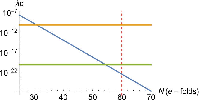
Figure 1: Relation between the physical e-folds $N$ (Jordan frame) and the collapse parameter $\lambda_{c}(s^{-1})$. We can appreciate the regions where $\lambda_{c}$ in permitted according to Carlesso et al. [2016]. Also, the central value of 60 e-folds correspond to a value of $\lambda_{c}(s^{-1})\simeq 10^{-22}$.

Thus, considering the previous equation and focusing on the equality in (50), we obtain a direct relation between the number of physical e-folds and the collapse parameter $\tilde{\lambda}_{c}$ which is presented in Figure 1. Also the upper and lower bounds on the standard CSL collapse parameter are indicated, which according to Carlesso et al. [2016] characterizes the experimental constraints as extracted directly from laboratory tests involving non-relativistic many particle systems. These constraints place the collapse parameter in the range $10^{-20}$ to $10^{-10}$ that according to our analysis correspond to a range of 30 – 55 e-folds.

Also, according to Figure 1, for inflation to last for $N\simeq 60$ e-folds in the physical frame, the collapse rate would need to be $\tilde{\lambda}_{c}\simeq 10^{-22}\ \text{s}^{-1}$ .

V Discussion

The inflationary paradigm has been quite successful in estimating the shape and scale of the primordial spectrum of fluctuations, which ultimately are seen in temperature patterns in the CMB, with some of its dominant features also identified in the large scale distribution of galaxies. However, as we have emphasized throughout this work, the standard treatment does not really account for the emergence of the primordial inhomogeneities. The new approach that has been proposed subjects the quantum dynamics of the field associated with the fluctuations of the inflaton to a collapse mechanism, specifically described through an adaptation to cosmology of the CSL theory.

By considering this new approach for treating the quantum perturbations of the inflation field, we are able to relax the conditions that strongly constrain Higgs inflation, maintaining the analysis in the regime where perturbation theory can still be considered valid.

We have been able to solve the problem in a natural way while allowing the non-minimal coupling constant $\xi$ introduced in these contexts to be less than 1. This has been achieved while considering a range of values of the collapse rate $\lambda_{c}$ which, according to Figure 1, are related directly to the maximum number $N$ of e-folds expected in the corresponding situation (and which are compatible with $\xi<1$ ). The range that is considered as viable, in view of experimental constrains and the suitability of the theories in resolving the measurement problem, for $\lambda_{c}$ results in a range of 30 – 55 e-folds, which is very close to the commonly assumed range of 50 – 60 e-folds, as considered for instance in equation 24 of Ade et al. [2014].

The fact that we have considered the collapse dynamics as parametrized in terms of the cosmological time associated with the Einstein frame can be regarded as indicating that the collapse parameter would depend on “time” when the evolution is expressed in terms of the cosmological time associated with the Jordan frame. This, in turn, might be seen as tied to the proposals made in recent papers suggesting that the collapse rate might depend on curvature Modak and Sudarsky [2017], Okon and Sudarsky [2014]. Such feature would be relevant for cosmological applications because, during the inflationary regime, the Universe’s curvature would have been quite different from that prevailing in the laboratory conditions to which the relevant bounds on $\lambda_{c}$ do apply. Thus, the inclusion of the novel idea in the analysis could be justified and be relevant in the establishment of the viability for Higgs-Inflation and the adjustment of the non-minimal coupling constant $\xi$ in the context of these proposals.

In summary, we have considered a simple version of the incorporation of the self-induced collapse of the wave function as a mechanism to generate, during the inflationary epoch the actual primordial inhomogeneities and anisotropies which are supposed to seed the structures in the Universe. By considering the incorporation of collapse theories into the picture, we were able to reassess the prospects that the Higgs field might be the field driving inflation, allowing to bypass the problems that afflict the standard accounts of Higgs inflation and which constitute the main reason to consider it unviable. As a byproduct, we found an interesting relationship between the parameter $\lambda_{c}$ characterizing the (fixed) collapse rate of the CSL collapse theory with the maximum number of e-folds allowed by the model.

VI Acknowledgments

This research project was supported CONACyT fellowship during S. R.’s PhD program.

D.S. is supported in part by the CONACYT grant No. 101712. and by UNAM-PAPIIT grant IN107412.

Appendix A Estimates of physical quantities

In order to relate the value of the collapse rate $\lambda_{c}$ to the expected value for the amplitude of the power spectrum of primordial inhomogeneities, we need to estimate the values of the conformal time $\eta$ at which inflation ends, $-\tau$, and starts, $-\mathcal{T}$. Recalling that the temperature of radiation scales like $1/a$, and assuming that the effective temperature at the end of inflation corresponds to the GUT scale given by $10^{15}$ GeV and the radiation temperature today is $2.7\ \text{K}=2.4\times 10^{13}$ GeV, we can estimate the scale factor $a(-\tau)$ according to

$$\frac{T(\text{today})}{T(-\tau)}=\frac{2.4\times 10^{-13}\ \text{GeV}}{10^{15}\ \text{GeV}}=\frac{a(-\tau)}{1}\ ,$$ (52)

yielding

$$a(-\tau)=2.4\times 10^{-28}\ .$$ (53)

In order to find the value of $\eta=-\tau$ that corresponds to the previous scale factor we can use the Friedmann equation

$$H^{2}=\frac{8\pi G}{3}V(\phi_{0})\ ,\quad V^{1/4}\sim\text{GUT scale}$$

to determine

$$H\simeq\frac{M^{2}_{GUT}}{3M_{P}}\simeq 10^{13}\ \text{GeV}\ ,$$ (54)

where $M_{P}=(8\pi G)^{-1/2}=2.435\times 10^{18}\ \text{GeV}$ and $M_{GUT}\simeq 10^{16}$.

Solving the classical equations of motion, the scale factor corresponding to the inflationary era is, to a good approximation,

$$a(\eta)=\frac{-1}{H\eta}\ ,$$ (55)

and so we can evaluate $a(\tau)$ to obtain $\tau=10^{-24}Mpc$ .

We can also compute the value of the conformal time at the start of inflation, for this we can assume that inflation lasts 60 e-folds, thus

$$\frac{\mathcal{T}}{\tau}=\frac{a(-\tau)}{a(-\mathcal{T})}=e^{60}\simeq 10^{26}\ ,$$ (56)

therefore $\mathcal{T}=10^{2}$ Mpc.

A.1 Estimates in the Einstein frame

The same estimations are needed in the section IV, but in the Einstein frame, since we have performed a conformal transformation in order to have the scalar inflaton field minimally coupled to gravity. The transformation from the physical frame (Jordan frame) to the Einstein frame is given by

$$d\tilde{s}^{2} = \tilde{a}^{2}(\tilde{\eta})[-d\tilde{\eta}^{2}+d\tilde{\vec{x}}^{2}]\ ,$$ (57)

$$= \Omega^{2}a^{2}(\eta)[-d\eta^{2}+d\vec{x}^{2}]\ ,$$

where the conformal factor $\Omega$ is given by

$$\Omega^{2}(h)=1+\frac{\xi h^{2}}{M_{P}^{2}}\ .$$ (58)

First we need to estimate the value of $\Omega$ at the end of inflation. So, we need the value of the field $h_{end}$ that we have already computed in equation (36),

$$h_{end}=\left(\frac{4}{3}\right)^{1/4}\frac{M_{P}}{\sqrt{\xi}}\ .$$ (59)

Therefore, the value of $\Omega$ at the end of inflation $(\eta=-\tau)$ is

$$\Omega(-\tau)\simeq\frac{3}{2}\ .$$ (60)

The next step is to use the Friedmann equation for the action given by (45), which is given by

$$\tilde{H}^{2}=\frac{8\pi G}{3}U(\chi)\ .$$ (61)

The value of the potential $U(\chi)$ is given by (33) and can be evaluated at $\chi_{end}=9.14M_{P}$, resulting in

$$\quad U(\chi_{end})\simeq\frac{\lambda M_{P}^{4}}{16\xi^{2}}\ ,$$ (62)

and, substituting into the previous equation, we have

$$\tilde{H}^{2}=\frac{1}{48}\frac{M_{P}^{2}}{\xi^{2}}\quad\Rightarrow\quad\tilde{H}\simeq\frac{7}{2\xi}\times 10^{17}\text{GeV}\ .$$ (63)

Now, we use the solution for the scale factor in this frame, given by

$$\tilde{a}(\tilde{\eta})=\frac{-1}{\tilde{H}\tilde{\eta}}\ ,\quad\tilde{a}(\tilde{\eta})=\Omega(\eta)a(\eta)\ ,$$ (64)

evaluating at the time when inflation ends, $\tilde{\eta}=-\tilde{\tau}$, we can solve for $\tilde{\tau}$, yielding

$$\tilde{\tau}=8\xi\times 10^{9}\ \text{GeV}^{-1}\ ,$$ (65)

where we have used the value of $a(-\tau)$ given by (52). With this results we can compute the value of the conformal time at the start of inflation assuming that inflation lasts N e-folds, thus we have

$$\frac{\tilde{\mathcal{T}}}{\tilde{\tau}}=\frac{\tilde{a}(-\tilde{\tau})}{\tilde{a}(-\tilde{\mathcal{T}})}=e^{\tilde{N}}\quad\Rightarrow\quad\tilde{\mathcal{T}}=8\xi e^{\tilde{N}}\times 10^{9}\ \text{GeV}^{-1}\ .$$ (66)

This approximation of $\mathcal{T}$ is used in Section IV to compute the fluctuation in the temperature.

References

- Hinshaw et al. [2013] G. Hinshaw et al. Nine-Year Wilkinson Microwave Anisotropy Probe (WMAP) Observations: Cosmological Parameter Results. Astrophys.J.Suppl., 208:19, 2013. doi: 10.1088/0067-0049/208/2/19.
- Ade [2014] P.A.R. Ade. Planck 2013 results. XXXI. Consistency of the Planck data. Astron.Astrophys., 571:A31, 2014. doi: 10.1051/0004-6361/201423743.
- Martin et al. [2014] Jérôme Martin, Christophe Ringeval, Roberto Trotta, and Vincent Vennin. The Best Inflationary Models After Planck. JCAP, 1403:039, 2014. doi: 10.1088/1475-7516/2014/03/039.
- Leon and Sudarsky [2013] Gabriel Leon and Daniel Sudarsky. Origin of Structure: Primordial Bispectrum without non-Gaussianities. 2013.
- Mukhanov et al. [1992] Viatcheslav F. Mukhanov, H. A. Feldman, and Robert H. Brandenberger. Theory of cosmological perturbations. Part 1. Classical perturbations. Part 2. Quantum theory of perturbations. Part 3. Extensions. Phys. Rept., 215:203–333, 1992. doi: 10.1016/0370-1573(92)90044-Z.
- Perez et al. [2006] Alejandro Perez, Hanno Sahlmann, and Daniel Sudarsky. On the quantum origin of the seeds of cosmic structure. Class. Quant. Grav., 23:2317–2354, 2006. doi: 10.1088/0264-9381/23/7/008.
- Weinberg [2008] Steven Weinberg. Cosmology. 2008. URL http://www.oup.com/uk/catalogue/?ci=9780198526827.
- Myrzakulov et al. [2015] Ratbay Myrzakulov, Sergei Odintsov, and Lorenzo Sebastiani. Inflationary universe from higher-derivative quantum gravity. Phys. Rev., D91(8):083529, 2015. doi: 10.1103/PhysRevD.91.083529.
- Barbon and Espinosa [2009] J. L. F. Barbon and J. R. Espinosa. On the Naturalness of Higgs Inflation. Phys. Rev., D79:081302, 2009. doi: 10.1103/PhysRevD.79.081302.
- Burgess et al. [2010] C. P. Burgess, Hyun Min Lee, and Michael Trott. Comment on Higgs Inflation and Naturalness. JHEP, 07:007, 2010. doi: 10.1007/JHEP07(2010)007.
- Hertzberg [2010] Mark P. Hertzberg. On Inflation with Non-minimal Coupling. JHEP, 11:023, 2010. doi: 10.1007/JHEP11(2010)023.
- Sudarsky [2013] Daniel Sudarsky. The SSC formalism and the collapse hypothesis for inflationary origin of the seeds of cosmic structure. J. Phys. Conf. Ser., 442:012071, 2013. doi: 10.1088/1742-6596/442/1/012071.
- Canate et al. [2013] Pedro Canate, Philip Pearle, and Daniel Sudarsky. Continuous spontaneous localization wave function collapse model as a mechanism for the emergence of cosmological asymmetries in inflation. Phys. Rev., D87(10):104024, 2013. doi: 10.1103/PhysRevD.87.104024.
- Sudarsky [2011] Daniel Sudarsky. Shortcomings in the Understanding of Why Cosmological Perturbations Look Classical. Int. J. Mod. Phys., D20:509–552, 2011. doi: 10.1142/S0218271811018937.
- Castagnino et al. [2014] Mario Castagnino, Sebastian Fortin, Roberto Laura, and Daniel Sudarsky. Interpretations of Quantum Theory in the Light of Modern Cosmology. 2014.
- Bell [1990] J. S. Bell. AGAINST ‘MEASUREMENT’. Phys. World, 3:33–40, 1990.
- Okon and Sudarsky [2014] Elias Okon and Daniel Sudarsky. Benefits of Objective Collapse Models for Cosmology and Quantum Gravity. Found. Phys., 44:114–143, 2014. doi: 10.1007/s10701-014-9772-6.
- Diez-Tejedor and Sudarsky [2012] Alberto Diez-Tejedor and Daniel Sudarsky. Towards a formal description of the collapse approach to the inflationary origin of the seeds of cosmic structure. JCAP, 1207:045, 2012. doi: 10.1088/1475-7516/2012/07/045.
- Bassi and Ghirardi [2003] Angelo Bassi and Gian Carlo Ghirardi. Dynamical reduction models. Phys. Rept., 379:257, 2003. doi: 10.1016/S0370-1573(03)00103-0.
- Guth [1981] Alan H. Guth. The Inflationary Universe: A Possible Solution to the Horizon and Flatness Problems. Phys. Rev., D23:347–356, 1981. doi: 10.1103/PhysRevD.23.347.
- Starobinsky [1979] Alexei A. Starobinsky. Spectrum of relict gravitational radiation and the early state of the universe. JETP Lett., 30:682–685, 1979. [Pisma Zh. Eksp. Teor. Fiz.30,719(1979)].
- Mott [1929] N. F. Mott. The wave mechanics of -ray tracks. Proceedings of the Royal Society of London A: Mathematical, Physical and Engineering Sciences, 126(800):79–84, 1929. ISSN 0950-1207. doi: 10.1098/rspa.1929.0205. URL http://rspa.royalsocietypublishing.org/content/126/800/79.
- Pearle [2012] Philip Pearle. Collapse Miscellany. arXiv.org, September 2012.
- Martin et al. [2012] Jerome Martin, Vincent Vennin, and Patrick Peter. Cosmological Inflation and the Quantum Measurement Problem. Phys. Rev., D86:103524, 2012. doi: 10.1103/PhysRevD.86.103524.
- Das et al. [2013] Suratna Das, Kinjalk Lochan, Satyabrata Sahu, and T. P. Singh. Quantum to classical transition of inflationary perturbations: Continuous spontaneous localization as a possible mechanism. Phys. Rev., D88(8):085020, 2013. doi: 10.1103/PhysRevD.89.109902,10.1103/PhysRevD.88.085020. [Erratum: Phys. Rev.D89,no.10,109902(2014)].
- Page and Geilker [1981] Don N. Page and C. D. Geilker. Indirect Evidence for Quantum Gravity. Phys. Rev. Lett., 47:979–982, 1981. doi: 10.1103/PhysRevLett.47.979.
- Mukhanov [2005] V. Mukhanov. Physical Foundations of Cosmology. Cambridge University Press, Oxford, 2005. ISBN 0521563984, 9780521563987. URL http://www-spires.fnal.gov/spires/find/books/www?cl=QB981.M89::2005.
- Leon and Sudarsky [2010] Gabriel Leon and Daniel Sudarsky. The Slow roll condition and the amplitude of the primordial spectrum of cosmic fluctuations: Contrasts and similarities of standard account and the ’collapse scheme’. Class. Quant. Grav., 27:225017, 2010. doi: 10.1088/0264-9381/27/22/225017.
- Ade et al. [2014] P. A. R. Ade et al. Planck 2013 results. XXII. Constraints on inflation. Astron. Astrophys., 571:A22, 2014. doi: 10.1051/0004-6361/201321569.
- Ghirardi et al. [1987] G. C. Ghirardi, A. Rimini, and T. Weber. On Disentanglement of Quantum Wave Functions: Answer to a Comment on ‘Unified Dynamics for Microscopic and Macroscopic Systems’. Phys. Rev., D36:3287, 1987. doi: 10.1103/PhysRevD.36.3287.
- Fakir and Unruh [1990] R Fakir and W G Unruh. Improvement on cosmological chaotic inflation through nonminimal coupling. Physical Review D, 41(6):1783–1791, 1990.
- Bezrukov and Shaposhnikov [2008a] Fedor Bezrukov and Mikhail Shaposhnikov. The Standard Model Higgs boson as the inflaton. Physics Letters B, 659(3):703–706, 2008a.
- Bezrukov and Shaposhnikov [2008b] Fedor L. Bezrukov and Mikhail Shaposhnikov. The Standard Model Higgs boson as the inflaton. Phys. Lett., B659:703–706, 2008b. doi: 10.1016/j.physletb.2007.11.072.
- Bezrukov [2013] Fedor Bezrukov. The Higgs field as an inflaton. Class. Quant. Grav., 30:214001, 2013. doi: 10.1088/0264-9381/30/21/214001.
- Burgess et al. [2009] C. P. Burgess, Hyun Min Lee, and Michael Trott. Power-counting and the Validity of the Classical Approximation During Inflation. JHEP, 09:103, 2009. doi: 10.1088/1126-6708/2009/09/103.
- Lerner and McDonald [2010] Rose N. Lerner and John McDonald. Higgs Inflation and Naturalness. JCAP, 1004:015, 2010. doi: 10.1088/1475-7516/2010/04/015.
- Atkins and Calmet [2011] Michael Atkins and Xavier Calmet. On the unitarity of linearized General Relativity coupled to matter. Phys. Lett., B695:298–302, 2011. doi: 10.1016/j.physletb.2010.10.049.
- Bezrukov and Gorbunov [2013] F. Bezrukov and D. Gorbunov. Light inflaton after LHC8 and WMAP9 results. JHEP, 07:140, 2013. doi: 10.1007/JHEP07(2013)140.
- Carlesso et al. [2016] M. Carlesso, A. Bassi, P. Falferi, and A. Vinante. Experimental bounds on collapse models from gravitational wave detectors. Phys. Rev., D94(12):124036, 2016. doi: 10.1103/PhysRevD.94.124036.
- Modak and Sudarsky [2017] Sujoy K. Modak and Daniel Sudarsky. Modelling non-paradoxical loss of information in black hole evaporation. Fundam. Theor. Phys., 187:303–316, 2017. doi: 10.1007/978-3-319-51700-1˙18.