DESY 17–188, DO-TH 17/31, TTK-17-36, NIKHEF 2017-059.
Heavy quark form factors at two loops in perturbative QCD

Abstract

We present the results for heavy quark form factors at two-loop order in perturbative QCD for different currents, namely vector, axial-vector, scalar and pseudo-scalar currents, up to second order in the dimensional regularization parameter. We outline the necessary computational details, ultraviolet renormalization and corresponding universal infrared structure.

PACS number

1 Introduction

The abundance of top quark pair production at high energy colliders provides important precision tests, with a strong potential for beyond the Standard Model (BSM) physics scenarios. The top quark, as the heaviest particle of the SM, has not been explored at high precision yet. Hence, detailed studies of this channel at future linear or circular electron-positron colliders is a crucial topic, which is likewise the case for the LHC. In order to match the experimental accuracy, precise predictions are required on the theoretical side as well. Furthermore, the form factors involving heavy quarks play an important role in determining various physical quantities concerning top quark pair production. The vector and axial vector massive form factors are important building blocks for the forward-backward asymmetry in the production of bottom or top quarks at electron-positron colliders. The decay of a scalar or pseudo-scalar particle to a pair of heavy quarks also could play a very important role in shedding light on the quantum nature of the Higgs boson. There are also static quantities like the anomalous magnetic moment, which receive contributions from such massive form factors. For these reasons, phenomenology and higher order Quantum chromodynamics (QCD) corrections to these form factors have gained much attention during the last decade.

A plethora of works [1, 2, 3, 4, 5, 6, 7, 8, 9, 10, 11, 12, 13, 14, 15, 16, 17] was followed by a series of papers obtaining the two-loop QCD corrections for the vector form factor [18], the axial-vector form factor [19], the anomaly contributions [20] and the scalar and pseudo-scalar form factors [21]. An independent cross-check of the vector form factor has been performed in [22] with the addition of the ${\mathcal{O}}(\varepsilon)$ contribution, where $\varepsilon=\frac{(4-D)}{2}$, $D$ being the space-time dimension. Recently, the calculation of a subset of the three-loop master integrals [23] has made it possible to obtain the vector form factor at three loops [24] in the color-planar limit. While the main goal is to compute the complete three-loop corrections for the form factors, the ${\cal O}(\varepsilon)$ pieces at two-loop order are necessary ingredients. Additionally, computing the master integrals with a different technique to the required order in $\varepsilon$ and cross-checking the available results in the literature are also motivating factors. In [25], we compute the contributions to the massive form factors up to ${\cal O}(\varepsilon^{2})$ for different currents, namely, vector, axial-vector, scalar and pseudo-scalar currents, which serve as input for ongoing and future 3- and 4-loop calculations.

2 The heavy quark form factors

We consider the decay of a virtual massive boson of momentum $q$ into a pair of heavy quarks of mass $m$, momenta $q_{1}$ and $q_{2}$, and color $c$ and $d$, through a vertex $X_{cd}$, where $X_{cd}=\Gamma^{\mu}_{V,cd},\Gamma^{\mu}_{A,cd},\Gamma_{S,cd}$ and $\Gamma_{P,cd}$ indicate a vector boson, an axial-vector boson, a scalar and a pseudo-scalar, respectively. $q^{2}$ is the center of mass energy squared and we define the dimensionless variable $s=\frac{q^{2}}{m^{2}}\,.$ To eliminate square-roots, we introduce another dimensionless variable $x$ defined by

$$s=-\frac{(1-x)^{2}}{x}\,.$$ (1)

The amplitudes take the following general form

$$\bar{u}_{c}(q_{1})X_{cd}v_{d}(q_{2})\,,$$ (2)

where $\bar{u}_{c}(q_{1})$ and $v_{d}(q_{2})$ are the bispinors of the quark and the anti-quark, respectively. We denote the corresponding UV renormalized form factors by $F_{I}$, $I=V,A,S,P$. They are expanded in the strong coupling constant ($\alpha_{s}=g_{s}^{2}/(4\pi)$) as follows

$$F_{I}=\sum_{n=0}^{\infty}\left(\frac{\alpha_{s}}{4\pi}\right)^{n}F_{I}^{(n)}\,.$$ (3)

Studying the general Lorentz structure, one finds the following generic forms for the amplitudes. For the vector and axial-vector currents we find

$$\Gamma_{cd}^{\mu}=\Gamma_{V,cd}^{\mu}+\Gamma_{A,cd}^{\mu}=-i\delta_{cd} \Big{[}v_{Q}\Big{(}\gamma^{\mu}~{}F_{V,1}+\frac{i}{2m}\sigma^{\mu\nu}q_{\nu}~{}F_{V,2}\Big{)}$$

$$+a_{Q}\Big{(}\gamma^{\mu}\gamma_{5}~{}F_{A,1}+\frac{1}{2m}q^{\mu}\gamma_{5}~{}F_{A,2}\Big{)}\Big{]}$$ (4)

where $\sigma^{\mu\nu}=\frac{i}{2}[\gamma^{\mu},\gamma^{\nu}]$, $q=q_{1}+q_{2}$, and $v_{Q}$ and $a_{Q}$ are the SM vector and axial-vector couplings, respectively. For the scalar and pseudo-scalar currents, we find

$$\Gamma_{cd} =\Gamma_{S,cd}+\Gamma_{P,cd}=-\frac{m}{v}\delta_{cd}~{}\Big{[}s_{Q}\,F_{S}+ip_{Q}\gamma_{5}\,F_{P}\Big{]}\,,$$ (5)

where $v=(\sqrt{2}G_{F})^{-1/2}$ is the SM Higgs vacuum expectation value, with $G_{F}$ being the Fermi constant, $s_{Q}$ and $p_{Q}$ are the scalar and pseudo-scalar couplings, respectively.

To extract the form factors $F_{I,i},~{}I=V,A$, we multiply the following projectors on $\Gamma^{\mu}_{cd}$ and perform a trace over the spinor and color indices

$$P_{V,i} =\frac{i}{v_{Q}}\frac{\delta_{cd}}{N_{c}}\frac{\not{q}_{2}-m}{m}\Big{(}\gamma_{\mu}g_{V,i}^{1}+\frac{1}{2m}(q_{2\mu}-q_{1\mu})g_{V,i}^{2}\Big{)}\frac{\not{q}_{1}+m}{m}\,,$$

$$P_{A,i} =\frac{i}{a_{Q}}\frac{\delta_{cd}}{N_{c}}\frac{\not{q}_{2}-m}{m}\Big{(}\gamma_{\mu}\gamma_{5}g_{A,i}^{1}+\frac{1}{2m}(q_{1\mu}+q_{2\mu})\gamma_{5}g_{A,i}^{2}\Big{)}\frac{\not{q}_{1}+m}{m}\,.$$ (6)

$g_{I,i}^{k}\equiv g_{I,i}^{k}(d,s)$ are given in [18, 19]. $N_{c}$ denotes the number of colors, $C_{F}=\frac{N_{c}^{2}-1}{2N_{c}}$ and $C_{A}=N_{c}$ are the eigenvalues of the Casimir operators of the gauge group SU($N_{c}$) in the fundamental and the adjoint representation, respectively. The form factors $F_{S}$ and $F_{P}$ can be obtained from $\Gamma_{cd}$ through suitable projectors as given below and performing trace over the spinor and color indices

$$P_{S} =\frac{v}{2ms_{Q}}\frac{\delta_{cd}}{N_{c}}\frac{\not{q}_{2}-m}{m}\Bigg{(}-\frac{1}{(s-4)}\Bigg{)}\frac{\not{q}_{1}+m}{m}\,,$$

$$P_{P} =\frac{v}{2mp_{Q}}\frac{\delta_{cd}}{N_{c}}\frac{\not{q}_{2}-m}{m}\Bigg{(}-\frac{i}{s}\gamma_{5}\Bigg{)}\frac{\not{q}_{1}+m}{m}\,.$$ (7)

2.1 Renormalization

To regularize the unrenormalized form factors we use dimensional regularization [26] in $D=4-2\varepsilon$ space-time dimensions. To do so, it becomes important to define $\gamma_{5}$ in a proper manner within this regularization scheme. Based on the appearance of $\gamma_{5}$ in a $\gamma$-chain in the axial-vector and pseudo-scalar form factors, the Feynman diagrams can be subdivided into two categories: non-singlet contributions, where $\gamma_{5}$ is attached to open fermion lines and singlet contributions, where $\gamma_{5}$ is attached to a closed fermion loop. For the non-singlet case, we use an anticommuting $\gamma_{5}$ in $D$ space-time dimensions with $\gamma_{5}^{2}=1$, as it does not lead to any spurious singularities. In this case, a canonical Ward identity holds to this order, as described by Eq. (14). We follow the prescription presented in [27, 28], which mostly followed [26], for the $\gamma_{5}$’s in the singlet contributions. For each $\gamma_{5}$ in a fermion loop we use

$$\gamma_{5}=\frac{i}{4!}\epsilon_{\mu\nu\rho\sigma}\gamma^{\mu}\gamma^{\nu}\gamma^{\rho}\gamma^{\sigma},$$ (8)

where the Lorentz indices are $D$-dimensional. In the end, we are left with the product of two $\epsilon$-tensors which is expressed in terms of $D$-dimensional metric tensors. This prescription of $\gamma_{5}$ needs a special treatment during renormalization, as will be discussed later.

The ultraviolet (UV) renormalization is performed in a mixed scheme. We renormalize the heavy-quark mass and wave function in the on-shell (OS) scheme, while the strong coupling constant is renormalized in the modified minimal subtraction ($\overline{\rm MS}$) scheme [29, 30]. The corresponding renormalization constants are already known in the literature and are denoted by $Z_{m,{\rm OS}}$ [31, 32, 33], $Z_{2,{\rm OS}}$ [31, 32, 33] and $Z_{a_{s}}$ [34, 35, 36, 37, 38] for the heavy-quark mass, wave function and strong coupling constant, respectively. The renormalization of massive fermion lines has been taken care of by properly considering the counterterms. The singlet contributions demand extra care for renormalization. The singlet pieces of the axial-vector current are infrared (IR) finite but the chirality preserving part of them contains a UV pole which is renormalized by the multiplicative renormalization constant $Z_{J}$. Larin’s prescription [28] for $\gamma_{5}$, on the other hand, implies multiplication of a finite renormalization constant $Z_{5}^{fin}$ which ensures that the anomalous Ward identity Eq. (15), as shown below, is satisfied. We would like to note that the Ward identities are true for physical quantities and hence, the remaining finite renormalization due to $Z_{5}^{fin}$ has to be carried out in calculating finally the corresponding observable to which the corresponding form factor contributes. An additional heavy quark mass renormalization is needed for scalar and pseudo-scalar currents due to the presence of heavy-quark mass in the Yukawa coupling. The singlet piece of the pseudo-scalar vertex is both IR and UV finite, hence no additional renormalization is necessary.

2.2 Infrared structure

The IR singularities of the massive form factors can be factorized [39] as a multiplicative renormalization factor. The corresponding structure is constrained by the renormalization group equation (RGE),

$$F_{I}=Z(\mu)F_{I}^{fin}(\mu)$$ (9)

where $F_{I}^{fin}$ is finite as $\varepsilon\rightarrow 0$ and the RGE of $Z$ gives

$$\frac{d}{d\ln\mu}\ln Z(\varepsilon,x,m,\mu)=-\Gamma(x,m,\mu)\,.$$ (10)

Note that $Z$ does not carry any information ($I$) regarding the vertex. Here $\Gamma$ denotes the massive cusp anomalous dimension, which is available up to three-loop level [40, 41, 42, 43]. Both $Z$ and $\Gamma$ can be expanded in a perturbative series in $\alpha_{s}$

$$Z=\sum_{n=0}^{\infty}\left(\frac{\alpha_{s}}{4\pi}\right)^{n}Z^{(n)}\,,\qquad\Gamma=\sum_{n=0}^{\infty}\left(\frac{\alpha_{s}}{4\pi}\right)^{n+1}\Gamma_{n}$$ (11)

and the solution for Eq. (10) is given by

$$Z=1+\left(\frac{\alpha_{s}}{4\pi}\right)\Bigg{[}\frac{\Gamma_{0}}{2\varepsilon}\Bigg{]}+\left(\frac{\alpha_{s}}{4\pi}\right)^{2}\Bigg{[}\frac{1}{\varepsilon^{2}}\Big{(}\frac{\Gamma_{0}^{2}}{8}-\frac{\beta_{0}\Gamma_{0}}{4}\Big{)}+\frac{\Gamma_{1}}{4\varepsilon}\Bigg{]}+{\cal O}(\alpha_{s}^{3})\,.$$ (12)

Eq. (12) correctly predicts the IR singularities for all massive form factors at two-loop level.

2.3 Anomaly and Ward identities

As stated earlier, the axial-vector and pseudo-scalar currents consist of two different contributions: non-singlet and singlet, depending on whether the vertex is attached to open fermion lines or a fermion loop, as

$$\Gamma_{A,cd}^{\mu}=\Gamma_{A,cd}^{\mu,ns}+\Gamma_{A,cd}^{\mu,s}\,,\quad\Gamma_{P,cd}=\Gamma_{P,cd}^{ns}+\Gamma_{P,cd}^{s}\,.$$ (13)

$ns$ and $s$ denote non-singlet and singlet cases, respectively. For the non-singlet case, we use anti-commutation of $\gamma_{5}$ and finally $\gamma_{5}^{2}=1$. This approach respects the chiral invariance and leaves us with the following Ward identity

$$q^{\mu}\Gamma_{A,cd}^{\mu,ns}=2m\Gamma_{P,cd}^{ns}\,.$$ (14)

The singlet contributions exhibit the ABJ anomaly [44, 45] which involves the truncated matrix element of the gluonic operator $G\tilde{G}$ between the vacuum and a pair of heavy quark states. Denoting its contribution by $\langle G\tilde{G}\rangle_{Q}$, we can immediately write down the anomalous Ward identity for the singlet case, as follows

$$q_{\mu}\Gamma_{A,cd}^{\mu,s}=2m\Gamma_{P,cd}^{s}-i\left(\frac{\alpha_{s}}{4\pi}\right)T_{F}\langle G\tilde{G}\rangle_{Q}\,.$$ (15)

The UV renormalization of the quantity $\langle G\tilde{G}\rangle_{Q}$ involves mixing of the gluonic operator with another operator $\partial_{\mu}\bar{\psi}\gamma^{\mu}\gamma_{5}\psi$, as discussed in [28, 46, 47].

3 Details of the computation

The computation of the two-loop form factors has been performed following the generic procedure. We have used QGRAF [48] to generate the Feynman diagrams. The output has then been processed using FORM [49, 50] to perform the Lorentz, Dirac and color algebra. Specifically we use the FORM package color [51] for color algebra. The diagrams have been expressed in terms of a linear combination of a large set of scalar integrals. These integrals have been reduced to a set of master integrals (MIs) using integration by parts identities (IBPs) [52, 53, 54, 55, 56, 57, 58] with the help of the program Crusher [59]. The diagrams have been matched to the different topologies defined in Crusher using the codes Q2e/Exp [60, 61]. Now, after performing the reductions, all that remains to be done is to compute the MIs. We follow both the method of differential equations and the method of difference equations to achieve this.

3.1 Method of differential equations

We have obtained the two-loop MIs contributing to massive form factors as Laurent expansions in $\varepsilon$ by means of the standard differential equation method [62, 63, 64, 65, 66, 67]. This technique has already been applied to such type of integrals at two and three loops in [68, 69, 23]. In this work, we have calculated the two-loop MIs up to sufficient order in $\varepsilon$ to obtain $O(\varepsilon^{2})$ accuracy in the form factors. We have derived a system of coupled linear differential equations by taking derivative of each MI w.r.t $x$ and then using IBPs again with help of Crusher. The system can then be expanded order-by-order in the parameter $\varepsilon$. The expanded system simplifies greatly and can be arranged mostly in a block triangular form except for a few $2\times 2$ sub-systems, for which we first decouple them and use the variation of constants to solve. Generically, we solve the whole system in a bottom-up approach i.e. first solving the simplest sectors and then moving up in the chain of sub-systems. These steps have been automated and results have been obtained efficiently using a minimal set of independent harmonic polylogarithms (HPLs) by means of the Mathematica packages Sigma [70, 71] and HarmonicSums [72, 73, 74, 75, 76, 77].

Now what remains is to obtain the appropriate boundary conditions. As noticed earlier in [68, 69], the analytic structure of the MIs puts strong constraints on the choice of integration constants. For most of the MIs, we determine the boundary conditions by demanding regularity of the functions at $x=1$. However, some MIs are characterized by a branch cut at $x=1$ and for such cases, we have matched the general solutions of the differential equations with asymptotic expansions of the corresponding integrals around $x\rightarrow 1$.

3.2 Method of difference equations

We have considered the method of difference equation as an alternative way to compute the MIs. The idea [65] is to write the integrals in series expansion of $y=(1-x)$ and then use the differential equations to derive difference equations satisfied by the coefficients of the series. In the non-singlet case, considering the fact that the MIs are regular at $x=1$, we can therefore write

$$J_{i}(y)=\sum_{n=0}^{\infty}\sum_{j=-2}^{r}\varepsilon^{j}C_{i,j}(n)y^{n}\,.$$ (16)

On the other hand, for the singlet case, some integrals have a branch cut at $x=1$ which actually shows up as $\ln(1-x)\equiv\ln(y)$. Henceforth, we include powers of these logarithms in the expansion of these integrals as [78]

$$K_{i}(y)=\sum_{n=0}^{\infty}\sum_{k=0}^{3}\sum_{j=-2}^{r}\varepsilon^{j}C_{i,j,k}(n)\ln^{k}(y)y^{n}.$$ (17)

Using the system of differential equations, we have obtained a system of difference equations for the coefficients $C_{i,j}$ and $C_{i,j,k}$. This system now can be solved with proper initial conditions in the same manner as for the system of differential equations and finally we have obtained the MIs in terms of harmonic sums and generalized harmonic sums and after performing the sums, in terms of HPLs. The whole procedure has been automated using Sigma, EvaluateMultiSums, SumProduction [79] and HarmonicSums.

4 Results

The analytic results for all two-loop UV renormalized form factors $F_{I}$, $I=V,A,S,P$ up to ${\cal O}(\varepsilon^{2})$ are presented as an attachment anci.m with the arXiv preprint [25]. The results up to ${\cal O}(\varepsilon)$ are printed in the appendix of [25].

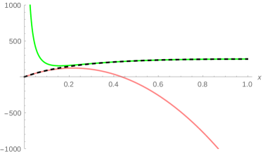
Figure 1: $C_{A}C_{F}$ coefficient of ${\cal O}(\varepsilon)$ part of $F_{V,1}$ (left) and $F_{V,2}$ (right).

The behavior of the form factors in various kinematic regions also carries substantial importance. We therefore study them in the low energy, high energy and threshold regions which correspond to $x\rightarrow 1$, $x\rightarrow 0$ and $x\rightarrow-1$, respectively. We extensively use the packages Sigma and HarmonicSums for all the expansions. Below, we present a brief summary of all the expansions, and instead of printing the voluminous results here, we choose to plot some parts of them, namely the coefficient of $C_{A}C_{F}$ for the ${\cal O}(\varepsilon)$ piece of each of the form factors and the corresponding expansion in high and low energy regions. Fig. 1, Fig. 2 and Fig. 3 contain the corresponding terms for vector, axial-vector and scalar form factors, respectively. The notation for the figures is presented in the right part of Fig. 3.

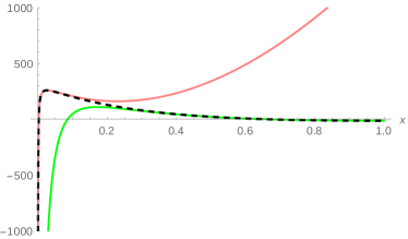
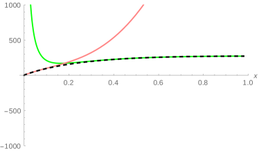
Figure 2: $C_{A}C_{F}$ coefficient of ${\cal O}(\varepsilon)$ part of $F_{A,1}$ (left) and $F_{A,2}$ (right).

Low energy region ($q^{2}\ll 4m^{2}$): The low energy limit of the space-like ($q^{2}<0$) form factors is given by $x\rightarrow 1$. To expand the HPLs, we redefine $x$ as $x=e^{i\phi}$ and expand them around $\phi=0$. Note that for $\phi\rightarrow 0$, $F_{V,1}=1$ and $F_{V,2}$ is finite and agrees with the anomalous magnetic moment of the top quark, as expected.

High energy region ($q^{2}\gg 4m^{2}$): The asymptotic or high energy limit is given by $x\rightarrow 0$. We expand the form factors up to ${\cal O}(x^{4})$. In the limit $x\rightarrow 0$, the chirality flipping form factors $F_{V,2}$ and $F_{A,2}$ vanish and the effect of $\gamma_{5}$ gets nullified implying $F_{V,1}=F_{A,1}$ and $F_{S}=F_{P}$.

Threshold region ($q^{2}\sim 4m^{2}$): In the threshold limit $q^{2}\sim 4m^{2}$ or $x\rightarrow-1$, we define the variable $\beta=\sqrt{1-\frac{4m^{2}}{q^{2}}}$ and expand the form factors around $\beta=0$ up to ${\cal O}(\beta^{2})$.

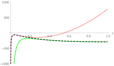
Figure 3: $C_{A}C_{F}$ coefficient of ${\cal O}(\varepsilon)$ part of $F_{S}$ (left) and labels for all plots.

4.1 Checks

We explicitly check our results by comparing them to the ones available in the literature. Except a difference in an overall factor due to different renormalization schemes and another difference in the wave function renormalization ($Z_{2,{\rm OS}}$), we agree with both the bare and UV renormalized results in [18, 19, 21] up to ${\cal O}(\varepsilon^{0})$ for all the form factors except the singlet parts of axial-vector form factors. While the bare singlet contributions for axial-vector currents also match with the results in [20], we find a mismatch of terms which are polynomial in $x$ for the renormalized contributions. We also compare the ${\cal O}(\varepsilon)$ pieces for the two-loop vector form factors $F_{V,1}^{(2)}$ and $F_{V,2}^{(2)}$ with the results presented in [22] and find a difference of the following term, as has also been mentioned in [24],

$$-C_{F}C_{A}\Bigg{[}\varepsilon\Big{\{}\frac{1037x^{3}}{(1+x)^{6}}\Big{\}}\Bigg{]}\,.$$ (18)

We cross-checked the vector form factors, the exact ones and also their expansions in different regions, presented in [24] up to ${\cal O}(\varepsilon)$ in the color-planar limit. We also compare with predictions of the vector form factor $F_{V,1}$ in the high energy limit as given in [22] considering the evolution equations.

5 Conclusion

To shed more light on the Higgs mechanism and electro-weak symmetry breaking, a precise determination of the properties of the top quark, the heaviest SM particle, is needed. A future electron-positron collider can reach high precision and hence an equal theory prediction is much required. In a similar way this also applies to the LHC for its high luminosity phase. In [25], we compute up to ${\cal O}(\varepsilon^{2})$ contributions to the heavy quark form factors for vector, axial-vector, scalar and pseudo-scalar currents at two-loop level. These contributions constitute an important part in three-loop results and also contribute to potential future 4-loop calculations. Additionally, they serve as a cross-check of earlier results available in the literature.

References

- [1] E. Braaten and J. P. Leveille Phys. Rev. D22 (1980) 715.
- [2] N. Sakai Phys. Rev. D22 (1980) 2220.
- [3] T. Inami and T. Kubota Nucl. Phys. B179 (1981) 171–188.
- [4] M. Drees and K.-i. Hikasa Phys. Lett. B240 (1990) 455. [Erratum: Phys. Lett.B262,497(1991)].
- [5] A. B. Arbuzov, D. Yu. Bardin, and A. Leike Mod. Phys. Lett. A7 (1992) 2029–2038. [Erratum: Mod. Phys. Lett.A9,1515(1994)].
- [6] A. Djouadi, B. Lampe, and P. M. Zerwas Z. Phys. C67 (1995) 123–128.
- [7] G. Altarelli and B. Lampe Nucl. Phys. B391 (1993) 3–22.
- [8] V. Ravindran and W. L. van Neerven Phys. Lett. B445 (1998) 214–222.
- [9] S. Catani and M. H. Seymour JHEP 07 (1999) 023.
- [10] S. G. Gorishnii, A. L. Kataev, and S. A. Larin Sov. J. Nucl. Phys. 40 (1984) 329–334. [Yad. Fiz.40,517(1984)].
- [11] S. G. Gorishnii, A. L. Kataev, S. A. Larin, and L. R. Surguladze Phys. Rev. D43 (1991) 1633–1640.
- [12] L. R. Surguladze Phys. Lett. B338 (1994) 229–234.
- [13] L. R. Surguladze Phys. Lett. B341 (1994) 60–72.
- [14] S. A. Larin, T. van Ritbergen, and J. A. M. Vermaseren Phys. Lett. B362 (1995) 134–140.
- [15] K. G. Chetyrkin and A. Kwiatkowski Nucl. Phys. B461 (1996) 3–18.
- [16] R. Harlander and M. Steinhauser Phys. Rev. D56 (1997) 3980–3990.
- [17] R. V. Harlander and W. B. Kilgore Phys. Rev. D68 (2003) 013001.
- [18] W. Bernreuther, R. Bonciani, T. Gehrmann, R. Heinesch, T. Leineweber, P. Mastrolia, and E. Remiddi Nucl. Phys. B706 (2005) 245–324.
- [19] W. Bernreuther, R. Bonciani, T. Gehrmann, R. Heinesch, T. Leineweber, P. Mastrolia, and E. Remiddi Nucl. Phys. B712 (2005) 229–286.
- [20] W. Bernreuther, R. Bonciani, T. Gehrmann, R. Heinesch, T. Leineweber, and E. Remiddi Nucl. Phys. B723 (2005) 91–116.
- [21] W. Bernreuther, R. Bonciani, T. Gehrmann, R. Heinesch, P. Mastrolia, and E. Remiddi Phys. Rev. D72 (2005) 096002.
- [22] J. Gluza, A. Mitov, S. Moch, and T. Riemann JHEP 07 (2009) 001.
- [23] J. M. Henn, A. V. Smirnov, and V. A. Smirnov JHEP 12 (2016) 144.
- [24] J. Henn, A. V. Smirnov, V. A. Smirnov, and M. Steinhauser JHEP 01 (2017) 074.
- [25] J. Ablinger, A. Behring, J. Blmlein, G. Falcioni, A. De Freitas, P. Marquard, N. Rana, and C. Schneider. in preparation.
- [26] G. ’t Hooft and M. J. G. Veltman Nucl. Phys. B44 (1972) 189–213.
- [27] D. A. Akyeampong and R. Delbourgo Nuovo Cim. A17 (1973) 578–586.
- [28] S. A. Larin Phys. Lett. B303 (1993) 113–118.
- [29] G. ’t Hooft Nucl. Phys. B61 (1973) 455–468.
- [30] W. A. Bardeen, A. J. Buras, D. W. Duke, and T. Muta Phys. Rev. D18 (1978) 3998.
- [31] D. J. Broadhurst, N. Gray, and K. Schilcher Z. Phys. C52 (1991) 111–122.
- [32] K. Melnikov and T. van Ritbergen Nucl. Phys. B591 (2000) 515–546.
- [33] P. Marquard, L. Mihaila, J. H. Piclum, and M. Steinhauser Nucl. Phys. B773 (2007) 1–18.
- [34] D. J. Gross and F. Wilczek Phys. Rev. Lett. 30 (1973) 1343–1346.
- [35] H. D. Politzer Phys. Rev. Lett. 30 (1973) 1346–1349.
- [36] W. E. Caswell Phys. Rev. Lett. 33 (1974) 244.
- [37] D. R. T. Jones Nucl. Phys. B75 (1974) 531.
- [38] E. Egorian and O. V. Tarasov Teor. Mat. Fiz. 41 (1979) 26–32. [Theor. Math. Phys.41,863(1979)].
- [39] T. Becher and M. Neubert Phys. Rev. D79 (2009) 125004. [Erratum: Phys. Rev.D80,109901(2009)].
- [40] G. P. Korchemsky and A. V. Radyushkin Nucl. Phys. B283 (1987) 342–364.
- [41] G. P. Korchemsky and A. V. Radyushkin Phys. Lett. B279 (1992) 359–366.
- [42] A. Grozin, J. M. Henn, G. P. Korchemsky, and P. Marquard Phys. Rev. Lett. 114 no. 6, (2015) 062006.
- [43] A. Grozin, J. M. Henn, G. P. Korchemsky, and P. Marquard JHEP 01 (2016) 140.
- [44] S. L. Adler Phys. Rev. 177 (1969) 2426–2438.
- [45] J. S. Bell and R. Jackiw Nuovo Cim. A60 (1969) 47–61.
- [46] M. F. Zoller JHEP 07 (2013) 040.
- [47] T. Ahmed, T. Gehrmann, P. Mathews, N. Rana, and V. Ravindran JHEP 11 (2015) 169.
- [48] P. Nogueira J. Comput. Phys. 105 (1993) 279–289.
- [49] J. A. M. Vermaseren arXiv:math-ph/0010025 [math-ph].
- [50] M. Tentyukov and J. A. M. Vermaseren Comput. Phys. Commun. 181 (2010) 1419–1427.
- [51] T. van Ritbergen, A. N. Schellekens, and J. A. M. Vermaseren Int. J. Mod. Phys. A14 (1999) 41–96.
- [52] J. Lagrange Miscellanea Taurinensis t. II (1760-61) 263.
- [53] C. Gauss Commentationes societas scientiarum Gottingensis recentiores III (1813) 5–7.
- [54] G. Green Nottingham III (1828) 1–115.
- [55] M. Ostrogradski Mem. Ac. Sci. St. Peters. 6 (1831) 39.
- [56] K. G. Chetyrkin, A. L. Kataev, and F. V. Tkachov Nucl. Phys. B174 (1980) 345–377.
- [57] K. G. Chetyrkin and F. V. Tkachov Nucl. Phys. B192 (1981) 159–204.
- [58] F. V. Tkachov Phys. Lett. 100B (1981) 65–68.
- [59] P. Marquard and D. Seidel. (unpublished).
- [60] R. Harlander, T. Seidensticker, and M. Steinhauser Phys. Lett. B426 (1998) 125–132.
- [61] T. Seidensticker 1999. arXiv:hep-ph/9905298 [hep-ph].
- [62] A. V. Kotikov Phys. Lett. B254 (1991) 158–164.
- [63] A. V. Kotikov Phys. Lett. B259 (1991) 314–322.
- [64] A. V. Kotikov Phys. Lett. B267 (1991) 123–127. [Erratum: Phys. Lett.B295,409(1992)].
- [65] E. Remiddi Nuovo Cim. A110 (1997) 1435–1452.
- [66] A. V. Kotikov pp. 150–174. 2010. arXiv:1005.5029 [hep-th].
- [67] J. M. Henn Phys. Rev. Lett. 110 (2013) 251601.
- [68] R. Bonciani, P. Mastrolia, and E. Remiddi Nucl. Phys. B661 (2003) 289–343. [Erratum: Nucl. Phys.B702,359(2004)].
- [69] R. Bonciani, P. Mastrolia, and E. Remiddi Nucl. Phys. B690 (2004) 138–176.
- [70] C. Schneider Sém. Lothar. Combin. 56 (2007) 1, article B56b.
- [71] C. Schneider arXiv:1304.4134 [cs.SC].
- [72] J. Ablinger PoS LL2014 (2014) 019.
- [73] J. Ablinger. 2009. arXiv:1011.1176 [math-ph].
- [74] J. Ablinger. 2012-04. arXiv:1305.0687 [math-ph].
- [75] J. Ablinger, J. Blmlein, and C. Schneider J. Math. Phys. 52 (2011) 102301.
- [76] J. Ablinger, J. Blmlein, and C. Schneider J. Math. Phys. 54 (2013) 082301.
- [77] J. Ablinger, J. Blmlein, C. G. Raab, and C. Schneider J. Math. Phys. 55 (2014) 112301.
- [78] A. Maier, P. Maierhofer, and P. Marquard Nucl. Phys. B797 (2008) 218–242.
-
[79]
J. Ablinger, J. Blümlein, S. Klein and C. Schneider,
Nucl. Phys. Proc. Suppl. 205-206 (2010) 110
[arXiv:1006.4797 [math-ph]];
J. Blümlein, A. Hasselhuhn and C. Schneider, PoS (RADCOR 2011) 032 [arXiv:1202.4303 [math-ph]];
C. Schneider,Computer Algebra Rundbrief 53 (2013), 8;
C. Schneider, EvaluateMultiSums and SumProduction,” J. Phys. Conf. Ser. 523 (2014) 012037 [arXiv:1310.0160 [cs.SC]].