Cooperative data-driven distributionally robust optimization

Abstract

This paper studies a class of multiagent stochastic optimization problems where the objective is to minimize the expected value of a function which depends on a random variable. The probability distribution of the random variable is unknown to the agents, so each one gathers samples of it. The agents then aim to cooperatively find, using their data, a solution to the optimization problem with guaranteed out-of-sample performance. The approach is to formulate a data-driven distributionally robust optimization problem using Wasserstein ambiguity sets, which turns out to be equivalent to a convex program. We reformulate the latter as a distributed optimization problem and identify a convex-concave augmented Lagrangian function whose saddle points are in correspondence with the optimizers provided a min-max interchangeability criteria is met. Our distributed algorithm design then consists of the saddle-point dynamics associated to the augmented Lagrangian. We formally establish that the trajectories of the dynamics converge asymptotically to a saddle point and hence an optimizer of the problem. Finally, we provide a class of functions that meet the min-max interchangeability criteria. Simulations illustrate our results.

I Introduction

Stochastic optimization in the context of multiagent systems has numerous applications, such as target tracking, distributed estimation, and cooperative planning and learning. Solving stochastic optimization problems, in an exact sense, requires the knowledge of the probability distribution of the random variables. Even then, computing this optimizer is computationally burdensome because of the expectation operator. To mitigate this problem, researchers have studied numerous sample-based methods that provide tractable ways of approximating the optimizer. One of the concerns of such methods is obtaining out-of-sample performance, avoiding overfitting. The concern is more pressing when only a few samples are available, typically in applications where acquiring samples is expensive due to the size and complexity of the system or when decisions must be taken in real time, leaving less room for gathering many samples. Distributionally robust optimization (DRO) provides a regularization framework that guarantees good out-of-sample performance even when the data is disturbed and not sampled from the true distribution. Motivated by this, we consider here the task for a group of agents to collaboratively find a data-driven solution for a stochastic optimization problem using the tools provided by the DRO framework.

Literature review: Stochastic optimization is a classical topic [2]. To the large set of methods available to solve this type of problems, a recent addition is data-driven distributionally robust optimization, see e.g., [3, 4, 5, 6, 7] and references therein. In this setup, the distribution of the random variable is unknown and so, a worst-case optimization is carried over a set of distributions, termed ambiguity set. This worst-case optimization provides probabilistic performance bounds for the original stochastic optimization [3, 8] and overcomes the problem of overfitting. One way of designing the ambiguity sets is to consider the set of distributions that are close (in some distance metric over the space of distributions) to some reference distribution constructed from the available data. Depending on the metric, one gets different ambiguity sets with different performance bounds. Some popular metrics are $\phi$-divergence [9], Prohorov metric [10], and Wasserstein distance [3]. Here, we consider ambiguity sets defined using the Wasserstein metric. In [4], the ambiguity set is constructed with distributions that pass a goodness-of-fit test. In addition to data-driven methods, other works on distributionally robust optimization consider ambiguity sets defined using moment constraints [11, 12] and the KL-divergence distance [13]. Tractable reformulations for the data-driven DRO methods have been well studied [3, 5, 14]. However, designing coordination algorithms to find a data-driven solution when the data is gathered in a distributed way by a network of agents has not been investigated. This is the focus of this paper. Our work has connections with the growing body of literature on distribution optimization problems [15, 16, 17] and agreement-based algorithms to solve them, see e.g., [18, 19, 20, 21, 22, 23] and references therein.

Besides data-driven DRO, one can solve the stochastic optimization problem considered here via other sampling-based methods, see [24]. Among these, sample average approximation (SAA) and stochastic approximation (SA) have received much attention because of their simple implementation and finite-sample guarantees independent of the dimension of the uncertainty, see e.g. [2, Chapter 5] and [25]. However, such guarantees need not hold when the samples are corrupted and may require stricter assumptions on the cost function and the feasibility set. In contrast, the sample guarantees of the data-driven DRO method hold for more general settings, see e.g., [3, 8], but are (potentially) more conservative and do not scale well with the size of the uncertainty parameter. Additionally, the complexity of solving a data-driven DRO is often worse than that of the SAA and SA methods.

Statement of contributions: Our starting point is a multiagent stochastic optimization problem involving the minimization of the expected value of an objective function with a decision variable and a random variable as arguments. The probability distribution of the random variable is unknown and instead, agents collect a finite set of samples of it. Given this data, each agent can individually find a data-driven solution of the stochastic optimization. However, agents wish to cooperate to leverage on the data collected by everyone in the group. Our approach consists of formulating a distributionally robust optimization problem over ambiguity sets defined as neighborhoods of the empirical distribution under the Wasserstein metric. The solution of this problem has guaranteed out-of-sample performance for the stochastic optimization. Our first contribution is the reformulation of the DRO problem to display a structure amenable to distributed algorithm design. We achieve this by augmenting the decision variables to yield a convex optimization whose objective function is the aggregate of individual objectives and whose constraints involve consensus among neighboring agents. Building on an augmented version of the associated Lagrangian function, we identify a convex-concave function which under a min-max interchangeability condition has the property that its saddle-points are in one-to-one correspondence with the optimizers of the reformulated problem. Our second contribution is the design of the saddle-point dynamics for the identified convex-concave Lagrangian function. We show that the proposed dynamics is distributed and provably correct, in the sense that its trajectories asymptotically converge to a solution of the original stochastic optimization problem. Our third contribution is the identification of two broad class of objective functions for which the min-max interchangeability holds. The first class is the set of functions that are convex-concave in the decision and the random variable, respectively. The second class is where functions are convex-convex and have some additional structure: they are either quadratic in the random variable or they correspond to the loss function of the least-squares problem. Finally, we illustrate our results in simulation.

II Preliminaries

This section introduces notation and basic notions on graph theory, convex analysis, and stability of discontinuous dynamical systems. A reader already familiar with these concepts can safely skip it.

II-1 Notation

Let , ${\mathbb{R}}_{\geq 0}$, and $\mathbb{Z}_{\geq 1}$ denote the set of real, nonnegative real, and positive integer numbers. The extended reals are denoted as $\overline{\mathbb{R}}=\real\cup\{-\infty,\infty\}$. For a positive integer $n\in\mathbb{Z}_{\geq 1}$, the set $[n]:=\{1,\dots,n\}$. We let $\|\cdot\|$ denote the $2$-norm on ⁿ. We use the notation $B_{\delta}(x):=\{y\in{}^{n}\;|\;\|x-y\|<\delta\}$. Given $x,y\in{}^{n}$, $x_{i}$ denotes the $i$-th component of $x$, and $x\leq y$ denotes $x_{i}\leq y_{i}$ for $i\in[n]$. For vectors $u\in{}^{n}$ and $w\in{}^{m}$, the vector $(u;w)\in{}^{n+m}$ denotes their concatenation. We use the shorthand notation $\mathbf{0}_{n}=(0,\ldots,0)\in{}^{n}$, $\mathbf{1}_{n}=(1,\ldots,1)\in{}^{n}$, and $\mathsf{I}_{n}\in{}^{n\times n}$ for the identity matrix. For $A\in{}^{n_{1}\times n_{2}}$ and $B\in{}^{m_{1}\times m_{2}}$, $A\otimes B\in{}^{n_{1}m_{1}\times n_{2}m_{2}}$ is the Kronecker product. The Cartesian product of $\{\SS_{i}\}_{i=1}^{n}$ is denoted by $\prod_{i=1}^{n}\SS_{i}:=\SS_{1}\times\dots\times\SS_{n}$. The interior of a set $\SS\subset{}^{n}$ is denoted by $\mathrm{int}(\SS)$. For a function $f:{}^{n}\times{}^{m}\to\real$, $(x,\xi)\mapsto f(x,\xi)$, we denote the partial derivative of $f$ with respect to the first argument by $\nabla_{x}f$ and with respect to the second argument by $\nabla_{\xi}f$. The higher-order derivatives follow the convention $\nabla_{x\xi}f=\frac{\partial^{2}f}{\partial x\partial\xi}$, $\nabla_{xx}f=\frac{\partial^{2}f}{\partial x^{2}}$, and so on. Given $V:\mathcal{X}\rightarrow{\mathbb{R}}_{\geq 0}$, we denote the $\delta$-sublevel set as $V^{-1}(\leq\delta):=\{x\in\mathcal{X}\;|\;V(x)\leq\delta\}$.

II-2 Graph theory

Following [26], an undirected graph, or simply a graph, is a pair $\mathcal{G}=(\mathcal{V},\mathcal{E})$, where $\mathcal{V}=[n]$ is the vertex set and $\mathcal{E}\subseteq\mathcal{V}\times\mathcal{V}$ is the edge set with the property that $(i,j)\in\mathcal{E}$ if and only if $(j,i)\in\mathcal{E}$. A path is an ordered sequence such that any ordered pair of vertices appearing consecutively is an edge. A graph is connected if there is a path between any pair of distinct vertices. Let $\mathcal{N}_{i}\subseteq\mathcal{V}$ denote the set of neighbors of vertex $i\in\mathcal{V}$, i.e., $\mathcal{N}_{i}=\{j\in\mathcal{V}\;|\;(i,j)\in\mathcal{E}\}$. A weighted graph is a triplet $\mathcal{G}=(\mathcal{V},\mathcal{E},\mathsf{A})$, where $(\mathcal{V},\mathcal{E})$ is a digraph and $\mathsf{A}\in\mathbb{R}^{n\times n}_{\geq 0}$ is the (symmetric) adjacency matrix of $\mathcal{G}$, with the property that $a_{ij}>0$ if $(i,j)\in\mathcal{E}$ and $a_{ij}=0$, otherwise. The weighted degree of $i\in[n]$ is $w_{i}=\sum_{j=1}^{n}a_{ij}$. The weighted degree matrix $\mathsf{D}$ is the diagonal matrix defined by $(\mathsf{D})_{ii}=w_{i}$, for all $i\in[n]$. The Laplacian matrix is $\mathsf{L}=\mathsf{D}-\mathsf{A}$. Note that $\mathsf{L}=\mathsf{L}^{\top}$ and $\mathsf{L}\mathbf{1}_{n}=0$. If $\mathcal{G}$ is connected, then zero is a simple eigenvalue of $\mathsf{L}$.

II-3 Convex analysis

Here we introduce elements from convex analysis following [27]. A set $C\subset{}^{n}$ is convex if $(1-\lambda)x+\lambda y\in C$ whenever $x\in C$, $y\in C$, and $\lambda\in(0,1)$. A vector $\varphi\in{}^{n}$ is normal to a convex set $C$ at a point $x\in C$ if $(y-x)^{\top}\varphi\leq 0$ for all $y\in C$. The set of all vectors normal to $C$ at $x$, denoted $N_{C}(x)$, is the normal cone to $C$ at $x$. The affine hull of $S\subset{}^{n}$ is the smallest affine space containing $S$,

$$\mathrm{aff}(S):=\big{\{}\sum_{i=1}^{k}\lambda_{i}x_{i}\;|\;k\in\mathbb{Z}_{\geq 1},x_{i}\in S,\lambda_{i}\in\real,\sum_{i=1}^{k}\lambda_{i}=1\big{\}}.$$

The relative interior of a convex set $C$ is the interior of $C$ relative to the affine hull of $C$. Formally,

$$\mathrm{ri}(C)\!:=\!\{x\!\in\!\mathrm{aff}(C)\;|\;\exists\epsilon>0,(x+\epsilon B_{1}(0))\cap(\mathrm{aff}(C))\!\subset C\}.$$

Given a convex set $C$, a vector $d$ is a direction of recession of $C$ if $x+\alpha d\in C$ for all $x\in C$ and $\alpha\geq 0$.

A convex function $f:{}^{n}\rightarrow\overline{\mathbb{R}}$ is proper if there exists $x\in{}^{n}$ such that $f(x)<+\infty$ and $f$ does not take the value $-\infty$ anywhere in ⁿ. The epigraph of $f$ is the set

$$\mathrm{epi}f:=\{(x,\lambda)\in({}^{n}\times\overline{\mathbb{R}})\;|\;\lambda\geq f(x)\}.$$

A function $f$ is closed if $\mathrm{epi}f$ is a closed set. The function $f$ is convex if and only if $\mathrm{epi}f$ is convex. For a closed proper convex function $f$, a vector $d$ is a direction of recession of $f$ if $(d,0)$ is a direction of recession of the set $\mathrm{epi}f$. Intuitively, it is the direction along which $f$ is monotonically non-increasing. If $f(x)\to+\infty$ whenever $\|x\|\to+\infty$, then $f$ does not have a direction of recession.

A function $F:\mathcal{X}\times\mathcal{Y}\rightarrow\overline{\mathbb{R}}$ is convex-concave (on $\mathcal{X}\times\mathcal{Y}$) if, given any point $(\tilde{x},\tilde{y})\in\mathcal{X}\times\mathcal{Y}$, $x\mapsto F(x,\tilde{y})$ is convex and $y\mapsto F(\tilde{x},y)$ is concave. When the space $\mathcal{X}\times\mathcal{Y}$ is clear from the context, we refer to this property as $F$ being convex-concave in $(x,y)$. A point $(x_{*},y_{*})\in\mathcal{X}\times\mathcal{Y}$ is a saddle point of $F$ over the set $\mathcal{X}\times\mathcal{Y}$ if $F(x_{*},y)\leq F(x_{*},y_{*})\leq F(x,y_{*})$, for all $x\in\mathcal{X}$ and $y\in\mathcal{Y}$. The set of saddle points of a convex-concave function $F$ is convex. Each saddle point is a critical point of $F$, i.e., if $F$ is differentiable, then $\nabla_{x}F(x_{*},z_{*})=0$ and $\nabla_{z}F(x_{*},z_{*})=0$. Additionally, if $F$ is twice differentiable, then $\nabla_{xx}F(x_{*},z_{*})\succeq 0$ and $\nabla_{zz}F(x_{*},z_{*})\preceq 0$. Given a convex-concave function $F:{}^{n}\times{}^{m}\rightarrow\overline{\mathbb{R}}$, define

$$\mathcal{X} :=\{x\in{}^{n}\;|\;F(x,y)<+\infty\text{ for all }y\in{}^{m}\},$$

$$\mathcal{Y} :=\{y\in{}^{m}\;|\;F(x,y)>-\infty\text{ for all }x\in{}^{n}\}.$$

The product set $\mathcal{X}\times\mathcal{Y}$ is called the effective domain of $F$. The sets $\mathcal{X}$, $\mathcal{Y}$ and so, $\mathcal{X}\times\mathcal{Y}$ are convex. Note that $F$ is finite on $\mathcal{X}\times\mathcal{Y}$. If $\mathcal{X}\times\mathcal{Y}$ is nonempty, then $F$ is called proper. If the following equality holds

$$\sup_{y\in\mathcal{Y}}\inf_{x\in\mathcal{X}}F(x,y)=\inf_{x\in\mathcal{X}}\sup_{y\in\mathcal{Y}}F(x,y),$$

then this common value is called the saddle value of $F$. The function $F$ is closed if for any $(x,y)\in\mathcal{X}\times\mathcal{Y}$, the functions $x\mapsto F(x,y)$ and $y\mapsto-F(x,y)$ are closed.

Theorem II.1.

(Existence of finite saddle value and saddle point [27, Theorem 37.3 & 37.6]): Let $F:{}^{n}\times{}^{m}\rightarrow\overline{\mathbb{R}}$ be a closed proper convex-concave function with effective domain $\mathcal{X}\times\mathcal{Y}\subset{}^{n}\times{}^{m}$. If the following conditions hold,

1. The convex functions $x\mapsto F(x,y)$ for $y\in\mathrm{ri}(\mathcal{Y})$ have no common direction of recession;

2. The convex functions $y\mapsto-F(x,y)$ for $x\in\mathrm{ri}(\mathcal{X})$ have no common direction of recession;

then the saddle value must be finite, there exists a saddle point of $F$ in the effective domain $\mathcal{X}\times\mathcal{Y}$ and the saddle value is attained at the saddle point.

II-4 Discontinuous dynamical systems

Here we present notions of discontinuous and projected dynamical systems from [28, 29, 30]. Let $f:{}^{n}\rightarrow{}^{n}$ be a Lebesgue measurable and locally bounded function, and consider

$$\dot{x}=f(x).$$ (1)

A map $\gamma:[0,T)\rightarrow{}^{n}$ is a (Caratheodory) solution of (1) on the interval $[0,T)$ if it is absolutely continuous on $[0,T)$ and satisfies $\dot{\gamma}(t)=f(\gamma(t))$ almost everywhere in $[0,T)$. We use the terms solution and trajectory interchangeably. A set $\SS\subset{}^{n}$ is invariant under (1) if every solution starting in $\SS$ remains in $\SS$. For a solution $\gamma$ of (1) defined on the time interval $[0,\infty)$, the omega-limit set $\Omega(\gamma)$ is defined by

$$\Omega(\gamma)=\{y\in{}^{n}\;|\;\text{there exists }\{t_{k}\}_{k=1}^{\infty}\subset[0,\infty)\text{ with }\\ \lim_{k\to\infty}t_{k}=\infty\text{ and }\lim_{k\to\infty}\gamma(t_{k})=y\}.$$

If the solution $\gamma$ is bounded, then $\Omega(\gamma)\neq\emptyset$ by the Bolzano-Weierstrass theorem [31, p. 33]. Given a continuously differentiable function $V:{}^{n}\rightarrow\real$, the Lie derivative of $V$ along (1) at $x\in{}^{n}$ is $\mathcal{L}_{f}V(x)=\nabla V(x)^{\top}f(x)$. The next result is a simplified version of [28, Proposition 3].

Proposition II.2.

(Invariance principle for discontinuous Caratheodory systems): Let $\SS\subset{}^{n}$ be compact and invariant. Assume that, for each point $x_{0}\in\SS$, there exists a unique solution of (1) starting at $x_{0}$ and that its omega-limit set is invariant too. Let $V:{}^{n}\rightarrow\real$ be a continuously differentiable map such that $\mathcal{L}_{f}V(x)\leq 0$ for all $x\in\SS$. Then, any solution of (1) starting at $\SS$ converges to the largest invariant set in $\mathrm{cl}(\{x\in\SS\;|\;\mathcal{L}_{f}V(x)=0\})$.

Projected dynamical systems are a particular class of discontinuous dynamical systems. Let $\mathcal{K}\subset{}^{n}$ be a closed convex set. Given a point $y\in{}^{n}$, the (point) projection of $y$ onto $\mathcal{K}$ is $\mathrm{proj}_{\mathcal{K}}(y)=\operatorname{argmin}_{z\in\mathcal{K}}\|z-y\|$. Note that $\mathrm{proj}_{\mathcal{K}}(y)$ is a singleton and the map $\mathrm{proj}_{\mathcal{K}}$ is Lipschitz on ⁿ with constant $L=1$ [32, Proposition 2.4.1]. Given $x\in\mathcal{K}$ and $v\in{}^{n}$, the (vector) projection of $v$ at $x$ with respect to $\mathcal{K}$ is

$$\Pi_{\mathcal{K}}(x,v)=\lim_{\delta\to 0^{+}}\frac{\mathrm{proj}_{\mathcal{K}}(x+\delta v)-x}{\delta}.$$

Given a vector field $f:{}^{n}\rightarrow{}^{n}$ and a closed convex polyhedron $\mathcal{K}\subset{}^{n}$, the associated projected dynamical system is

$$\dot{x}=\Pi_{\mathcal{K}}(x,f(x)),\quad x(0)\in\mathcal{K},$$ (2)

One can verify easily that for any $x\in\mathcal{K}$, there exists an element $\varphi_{x}$ belonging to the normal cone $N_{\mathcal{K}}(x)$ such that $\Pi_{\mathcal{K}}(x,f(x))=f(x)-\varphi_{x}$. In particular, if $x$ is in the interior of $\mathcal{K}$, then this element is the zero vector and we have $\Pi_{\mathcal{K}}(x,f(x))=f(x)$. At any boundary point of $\mathcal{K}$, the projection operator restricts the flow of the vector field $f$ such that the solutions of (2) remain in $\mathcal{K}$. Due to the projection, the dynamics (2) is in general discontinuous.

III Data-driven stochastic optimization

This section sets the stage for the formulation of our approach to deal with data-driven optimization in a distributed manner. The following material on data-driven stochastic optimization is taken from [3] and included here to provide a self-contained exposition. The reader familiar with these notions and tools can safely skip this section.

Let $(\Omega,\mathcal{F},P)$ be a probability space and $\xi$ be a random variable mapping this space to $({}^{m},B_{\sigma}({}^{m}))$, where $B_{\sigma}({}^{m})$ is the Borel $\sigma$-algebra on ^m. Let $\mathbb{P}$ and $\Xi\subseteq{}^{m}$ be the distribution and the support of the random variable $\xi$. Assume that $\Xi$ is closed and convex. Consider the stochastic optimization problem

$$\inf_{x\in\mathcal{X}}\mathbb{E}_{\mathbb{P}}[f(x,\xi)],$$ (3)

where $\mathcal{X}\subseteq{}^{n}$ is a closed convex set, $f:{}^{n}\times{}^{m}\rightarrow\real$ is a continuous function, and $\mathbb{E}_{\mathbb{P}}[\,\cdot\,]$ is the expectation under the distribution $\mathbb{P}$. Assume that $\mathbb{P}$ is unknown and so, solving (3) is not possible. However, we are given $N$ independently drawn samples $\widehat{\Xi}:=\{\widehat{\xi}^{\,k}\}_{k=1}^{N}\subset\Xi$ of the random variable $\xi$. Note that, until it is revealed, $\widehat{\Xi}$ is a random object with probability distribution $\mathbb{P}^{N}:=\prod_{i=1}^{N}\mathbb{P}$ supported on $\Xi^{N}:=\prod_{i=1}^{N}\Xi$. The objective is to find a data-driven solution of (3), denoted $\widehat{x}_{N}\in\mathcal{X}$, constructed using the dataset $\widehat{\Xi}$, that has desirable properties for the expected cost $\mathbb{E}_{\mathbb{P}}[f(\widehat{x}_{N},\xi)]$ under a new sample. The property we are looking for is the finite-sample guarantee given by

$$\mathbb{P}^{N}\Bigl{(}\mathbb{E}_{\mathbb{P}}[f(\widehat{x}_{N},\xi)]\leq\widehat{J}_{N}\Bigr{)}\geq 1-\beta,$$ (4)

where $\widehat{J}_{N}$ might also depend on the training dataset and $\beta\in(0,1)$ is the parameter which governs $\widehat{x}_{N}$ and $\widehat{J}_{N}$. The quantities $\widehat{J}_{N}$ and $1-\beta$ are referred to as the certificate and the reliability of the performance of $\widehat{x}_{N}$. The goal is to find a data-driven solution with a low certificate and a high reliability. To do so, we use the available information $\widehat{\Xi}$. The strategy is to determine a set $\widehat{\mathcal{P}}_{N}$ of probability distributions supported on $\Xi$ so that minimization of the worst-case cost over $\widehat{\mathcal{P}}_{N}$ results into a finite-sample guarantee. The set $\widehat{\mathcal{P}}_{N}$ is referred to as the ambiguity set. Once such a set is designed, the certificate $\widehat{J}_{N}$ is defined as the optimal value of the following distributionally robust optimization problem

$$\widehat{J}_{N}:=\inf_{x\in\mathcal{X}}\sup_{\mathbb{Q}\in\widehat{\mathcal{P}}_{N}}\mathbb{E}_{\mathbb{Q}}[f(x,\xi)].$$ (5)

This is the worst-case optimal value considering all distributions in $\widehat{\mathcal{P}}_{N}$. A good candidate for $\widehat{\mathcal{P}}_{N}$ is the set of distributions that are close (under a certain metric) to the uniform distribution on $\widehat{\Xi}$, termed the empirical distribution. Formally, the empirical distribution is

$$\widehat{\mathbb{P}}_{N}:=\frac{1}{N}\sum_{k=1}^{N}\delta_{\widehat{\xi}^{\,k}},$$ (6)

where $\delta_{\widehat{\xi}^{\,k}}$ is the unit point mass at $\widehat{\xi}^{\,k}$. Let $\mathcal{M}(\Xi)$ be the space of probability distributions $\mathbb{Q}$ supported on $\Xi$ with finite second moment, i.e., $\mathbb{E}_{\mathbb{Q}}[\|\xi\|^{2}]=\int_{\Xi}\|\xi\|^{2}\mathbb{Q}(d\xi)<+\infty$. The 2-Wasserstein metric $d_{W_{2}}:\mathcal{M}(\Xi)\times\mathcal{M}(\Xi)\rightarrow{\mathbb{R}}_{\geq 0}$ is

$$d_{W_{2}}(\mathbb{Q}_{1},\mathbb{Q}_{2})=\Bigl{(}\inf\Bigl{\{}\int_{\Xi^{2}}\|\xi_{1}- \xi_{2}\|^{2}\Pi(d\xi_{1},d\xi_{2})\Bigl{|}$$

$$\Pi\in\mathcal{H}(\mathbb{Q}_{1},\mathbb{Q}_{2})\Bigr{\}}\Bigr{)}^{\frac{1}{2}},$$ (7)

where $\mathcal{H}(\mathbb{Q}_{1},\mathbb{Q}_{2})$ is the set of all distributions on $\Xi\times\Xi$ with marginals $\mathbb{Q}_{1}$ and $\mathbb{Q}_{2}$. Given $\epsilon\geq 0$, we use the notation

$$\mathcal{B}_{\epsilon}(\widehat{\mathbb{P}}_{N}):=\{\mathbb{Q}\in\mathcal{M}(\Xi)\;|\;d_{W_{2}}(\widehat{\mathbb{P}}_{N},\mathbb{Q})\leq\epsilon\}$$ (8)

to define the set of distributions that are $\epsilon$-close to $\widehat{\mathbb{P}}_{N}$ under the defined metric. For an appropriately chosen radius $\epsilon$, the ambiguity set $\widehat{\mathcal{P}}_{N}=\mathcal{B}_{\epsilon}(\widehat{\mathbb{P}}_{N})$, plugged in the distributionally robust optimization (5), results into a finite-sample guarantee (4). There might be different ways of establishing this fact. For example, in [3], a bound for $\epsilon$ is provided under the assumption that $\mathbb{P}$ is light-tailed satisfying an exponential decay condition. The work [8], on the other hand, considers more general distributions and gives a different, potentially tighter, finite-sample guarantee. However, in [8], $f$ is assumed to be either quadratic or log-exponential loss function. The focus of this work is on the design of distributed algorithms to solve (5) with $\mathcal{B}_{\epsilon}(\widehat{\mathbb{P}}_{N})$ as the ambiguity set. To this end, the following tractable reformulation is key.

Theorem III.1.

(Tractable reformulation of (5)): Assume that for all $\tilde{\xi}\in\Xi$, $x\mapsto f(x,\tilde{\xi})$ is convex. Then, for $N\in\mathbb{Z}_{\geq 1}$, the optimal value of (5) with the choice $\widehat{\mathcal{P}}_{N}=\mathcal{B}_{\epsilon}(\widehat{\mathbb{P}}_{N})$ is equal to the optimum of the following convex optimization problem

$$\inf_{\lambda\geq 0,x\in\mathcal{X}}\Bigl{\{}\lambda\epsilon^{2}+\frac{1}{N}\sum_{k=1}^{N}\max_{\xi\in\Xi}\Bigl{(}f(x,\xi)-\lambda\|\xi-\widehat{\xi}^{\,k}\|^{2}\Bigr{)}\Bigr{\}}.$$

This result and its proof are similar to [3, Theorem 4.2] and its corresponding proof, respectively. While our metric is $2$-Wasserstein, the referred result’s is $1$-Wasserstein. Theorem III.1 shows that under mild conditions on the objective function, one can reformulate the distributionally robust optimization problem as a convex optimization problem. This result plays a key role in our forthcoming discussion. We note that the reformulation given in Theorem III.1 is valid under weaker set of conditions on $f$, as reported in [5] and [14]. We however avoid this generality as it complicates the design and analysis of the distributed algorithm.

IV Problem statement

Consider $n\in\mathbb{Z}_{\geq 1}$ agents communicating over an undirected weighted graph $\mathcal{G}=(\mathcal{V},\mathcal{E},\mathsf{A})$. The set of vertices are enumerated as $\mathcal{V}:=[n]$. Each agent $i\in[n]$ can send and receive information from its neighbors $\mathcal{N}_{i}$ in $\mathcal{G}$. Let $f:{}^{d}\times{}^{m}\rightarrow\real$, $(x,\xi)\mapsto f(x,\xi)$, be a continuously differentiable objective function. Assume that for any $\xi\in{}^{m}$, the map $x\mapsto f(x,\xi)$ is convex and that for any $x\in{}^{d}$, the map $\xi\mapsto f(x,\xi)$ is either convex or concave. Suppose that the set of $\xi\in{}^{m}$ for which $\mathbf{1}_{n}$ and $-\mathbf{1}_{n}$ are not a direction of recession for the convex function $x\mapsto f(x,\xi)$ is dense in ^m. As we progress, we stipulate additional conditions on $f$ as necessary. Assume that all agents know the objective function $f$. Given a random variable $\xi\in{}^{m}$ with support ^m and distribution $\mathbb{P}$, the original objective for the agents is to solve the following stochastic optimization problem

$$\inf_{x\in{}^{d}}\mathbb{E}_{\mathbb{P}}\bigl{[}f(x,\xi)\bigr{]}.$$ (9)

For simplicity, we optimize over ^d instead of some closed convex set $\mathcal{X}$. However, our proposed method can handle such generalization by assuming that each agent knows a subset of ^d such that the intersection of them all is $\mathcal{X}$. We assume that $\mathbb{P}$ is unknown to agents and instead, each agent has a certain number (at least one) of independent and identically distributed realizations of the random variable $\xi$. We denote the data available to agent $i$ by $\widehat{\Xi}_{i}$ that is assumed to be nonempty. Assume that $\widehat{\Xi}_{i}\cap\widehat{\Xi}_{j}=\emptyset$ for all $i,j\in[n]$ and let $\widehat{\Xi}=\cup_{i=1}\widehat{\Xi}_{i}$ containing $N$ samples be the available data set.

The goal for the agents is then to collectively find, in a distributed manner, a data-driven solution $\widehat{x}_{N}\in{}^{d}$ to approximate the optimizer of (9) with guaranteed performance bounds. To achieve this, we rely on the framework of distributionally robust optimization, cf. Section III. From Theorem III.1, a data-driven solution for (9) can be obtained by solving the following convex optimization problem

$$\inf_{\lambda\geq 0,x}\Bigl{\{}\!\lambda\epsilon^{2}\!+\!\frac{1}{N}\!\sum_{k=1}^{N}\max_{\xi\in{}^{m}}\Bigl{(}f(x,\xi)\!-\!\lambda\|\xi-\widehat{\xi}^{\,k}\|^{2}\Bigr{)}\!\Bigr{\}}.$$ (10)

The following is assumed to hold throughout the paper.

Assumption IV.1.

(Nontrivial feasibility and existence of finite optimizers of (10)): We assume that the set belonging to ${\mathbb{R}}_{\geq 0}\times{}^{d}$ where the objective function in (10) takes finite values has a nonempty interior. Further, we assume that there exists a finite optimizer $(x^{*},\lambda^{*})$ of (10). $\bullet$

The existence of finite optimizers is ensured if one of the set of conditions for such existence given in [33] are met. Note that each agent can individually find a data-driven solution to (9) by using only the data available to it in the convex formulation (10). However, such a solution in general will have an inferior out-of-sample guarantee as compared to the one obtained collectively. In the cooperative setting, agents aim to solve (10) in a distributed manner, that is

1. each agent $i$ has the information

   $$\mathcal{I}_{i}:=\{\widehat{\Xi}_{i},f,\epsilon,n,N\},$$ (11)

   where $\epsilon$ is the radius of the ambiguity set that agents agree upon beforehand,

2. each agent $i$ can only communicate with its neighbors $\mathcal{N}_{i}$ in the graph $\mathcal{G}$,

3. each agent $i$ does not share with its neighbors any element of the dataset $\widehat{\Xi}_{i}$ available to it, and

4. there is no central coordinator or leader that can communicate with all agents.

The challenge in solving (10) in a distributed manner lies in the fact that the data is distributed over the network and the optimizer $x^{*}$ depends on it all. Moreover, the inner maximization can be a nonconvex problem, in general. One way of solving (10) in a cooperative fashion is to let agents share their data with everyone in the network via some sort of flooding mechanism. This violates item (iii) of our definition of distributed algorithm given above. We specifically keep such methods out of scope due to two reasons. First, the data would not be private anymore, creating a possibility of adversarial action. Second, the communication burden of such a strategy is higher than our proposed distributed strategy when the size of the network and the dataset grows along the execution of the algorithm.

Our strategy to tackle the problem is organized as follows: in Section V we reformulate the problem (10) to obtain a structure which allows us in Section VI to propose our distributed algorithm. Section VII discusses a class of objective functions $f$ for which the distributed algorithm provably converges.

V Distributed problem formulation and saddle points

This section studies the structure of the optimization problem presented in Section IV with the ulterior goal of facilitating the design of a distributed algorithmic solution. Our first step is a reformulation of (10) that, by augmenting the decision variables of the agents, yields an optimization where the objective function is the aggregate of individual functions (that can be independently evaluated by the agents) and constraints which display a distributed structure. Our second step is the identification of a convex-concave function whose saddle points are the primal-dual optimizers of the reformulated problem under suitable conditions on the objective function $f$. This opens the way to consider the associated saddle-point dynamics as our candidate distributed algorithm. The structure of the original optimization problem makes this step particularly nontrivial.

Remark V.1.

(Alternative distributed algorithmic solutions): The optimization problem (10) can possibly be solved using other distributed methods. This might entail making use of alternative reformulations of (10). For instance, problem (10) can be written as a semi-infinite program, cf. [6], and then a distributed cutting-surface method can be designed following the centralized algorithm given in [6]. When $f$ is piecewise affine in $\xi$, (10) takes the form of a conic program (without the $\max$ operator in the objective), which can potentially be solved via primal-dual distributed solvers. Finally, following [8, 34], for certain $f$ (linear form or objective of LASSO or logistic regression), the problem (10) is equivalent to minimizing the empirical cost (expectation of cost function under empirical distribution) plus a regularizer term. For such cases, primal-dual distributed solvers may be a valid solution strategy. The advantage of the methodology proposed here is its generality, which does not require to write different algorithms for different cases depending on the form of $f$. $\bullet$

V-A Reformulation as distributed optimization problem

We have each agent $i\in[n]$ maintain a copy of $\lambda$ and $x$, denoted by $\lambda^{i}\in\real$ and $x^{i}\in{}^{d}$, respectively. Thus, the decision variables for $i$ are $(x^{i},\lambda^{i})$. For notational ease, let the concatenated vectors be $\lambda_{\operatorname{v}}:=(\lambda^{1};\dots;\lambda^{n})$, and $x_{\operatorname{v}}:=(x^{1};\dots;x^{n})$. Let $v_{k}\in[n]$ be the agent that holds the $k$-th sample $\widehat{\xi}^{\,k}$ of the dataset. Consider the following convex optimization problem

$$\underset{x_{\operatorname{v}},\lambda_{\operatorname{v}}\geq\mathbf{0}_{n}}{\min} \quad h(\lambda_{\operatorname{v}})+\frac{1}{N}\sum_{k=1}^{N}\max_{\xi\in{}^{m}}g_{k}(x^{v_{k}},\lambda^{v_{k}},\xi)$$ (12a)

$$\operatorname{subject\text{$\,\,$}to} \quad\mathsf{L}\lambda_{\operatorname{v}}=\mathbf{0}_{n},$$ (12b)

$$\quad(\mathsf{L}\otimes\mathsf{I}_{d})x_{\operatorname{v}}=\mathbf{0}_{nd},$$ (12c)

where $\mathsf{L}\in{}^{n\times n}$ is the Laplacian of the graph $\mathcal{G}$ and we have used the shorthand notation $h:{}^{n}\rightarrow\real$ for

$$h(\lambda_{\operatorname{v}}):=\frac{\epsilon^{2}(\mathbf{1}_{n}^{\top}\lambda_{\operatorname{v}})}{n}$$

and, for each $k\in[N]$, $g_{k}:{}^{d}\times\real\times{}^{m}\rightarrow\real$ for

$$g_{k}(x,\lambda,\xi):=f(x,\xi)-\lambda\|\xi-\widehat{\xi}^{\,k}\|^{2}.$$

The following result establishes the correspondence between the optimizers of (10) and (12), respectively.

Lemma V.2.

(One-to-one correspondence between optimizers of (10) and (12)): The following holds:

1. If $(x^{*},\lambda^{*})$ is an optimizer of (10), then $(\mathbf{1}_{n}\otimes x^{*},\lambda^{*}\mathbf{1}_{n})$ is an optimizer of (12).

2. If $(x_{\operatorname{v}}^{*},\lambda_{\operatorname{v}}^{*})$ is an optimizer of (12), then there exists an optimizer $(x^{*},\lambda^{*})$ of (10) such that $x_{\operatorname{v}}^{*}=\mathbf{1}_{n}\otimes x^{*}$ and $\lambda_{\operatorname{v}}^{*}=\lambda^{*}\mathbf{1}_{n}$.

Proof.

The proof follows by noting that $\mathcal{G}$ is connected and hence, (i) $\mathsf{L}\lambda_{\operatorname{v}}=\mathbf{0}_{n}$ if and only if $\lambda_{\operatorname{v}}=\alpha\mathbf{1}_{n}$, $\alpha\in\real$; and (ii) $(\mathsf{L}\otimes\mathsf{I}_{d})x_{\operatorname{v}}=\mathbf{0}_{nd}$ if and only if $x_{\operatorname{v}}=\mathbf{1}_{n}\otimes x$, $x\in{}^{d}$. $\blacksquare$

Note that constraints (12b) and (12c) force agreement and that each of their components is computable by an agent of the network using only local information. Moreover, the objective function (12a) can be written as $\sum_{i=1}^{n}J_{i}(x^{i},\lambda^{i},\widehat{\Xi}_{i})$, where

$$J_{i}(x^{i},\lambda^{i},\widehat{\Xi}_{i}):=\frac{\epsilon^{2}\lambda^{i}}{n}+\frac{1}{N}\sum_{k:\widehat{\xi}^{\,k}\in\widehat{\Xi}_{i}}\max_{\xi\in{}^{m}}g_{k}(x^{i},\lambda^{i},\xi),$$

for all $i\in[n]$. Therefore, the problem (12) has the adequate structure from a distributed optimization viewpoint: an aggregate objective function and locally computable constraints.

V-B Augmented Lagrangian and saddle points

Our next step is to identify an appropriate variant of the Lagrangian function of (12) with the following two properties: (i) it does not consist of an inner maximization, unlike the objective in (12a), and (ii) the primal-dual optimizers of (12) are saddle points of the newly introduced function. The availability of these two facts sets the stage for our ensuing algorithm design.

To proceed further, we first denote for convenience the objective function (12a) with $F:{}^{nd}\times{\mathbb{R}}_{\geq 0}^{n}\rightarrow\real$,

$$F(x_{\operatorname{v}},\lambda_{\operatorname{v}}):=h(\lambda_{\operatorname{v}})+\frac{1}{N}\sum_{k=1}^{N}\max_{\xi\in{}^{m}}g_{k}(x^{v_{k}},\lambda^{v_{k}},\xi).$$ (13)

Note that the Lagrangian of (12) is $L:{}^{nd}\times{\mathbb{R}}_{\geq 0}^{n}\times{}^{n}\times{}^{nd}\rightarrow\overline{\mathbb{R}}$,

$$L(x_{\operatorname{v}},\lambda_{\operatorname{v}},\nu,\eta)\!:=\!F(x_{\operatorname{v}},\lambda_{\operatorname{v}})+\nu^{\top}\mathsf{L}\lambda_{\operatorname{v}}+\eta^{\top}(\mathsf{L}\otimes\mathsf{I}_{d})x_{\operatorname{v}},$$ (14)

where $\nu\in{}^{n}$ and $\eta\in{}^{nd}$ are dual variables corresponding to the equality constraints (12b) and (12c), respectively. $L$ is convex-concave in $((x_{\operatorname{v}},\lambda_{\operatorname{v}}),(\nu,\eta))$ on the domain $\lambda_{\operatorname{v}}\geq\mathbf{0}_{n}$. The next result states that the duality gap for (12) is zero. The result is a consequence of [27, Corollary 28.22] and [27, Theorem 28.3] using the hypotheses of Assumption IV.1.

Lemma V.3.

(Min-max equality for $L$): The set of saddle points of $L$ over the domain $({}^{nd}\times{\mathbb{R}}_{\geq 0}^{n})\times({}^{n}\times{}^{nd})$ is nonempty and

$$\inf_{x_{\operatorname{v}},\lambda_{\operatorname{v}}\geq\mathbf{0}_{n}}\sup_{\nu,\eta}L(x_{\operatorname{v}},\lambda_{\operatorname{v}},\nu,\eta)=\sup_{\nu,\eta}\inf_{x_{\operatorname{v}},\lambda_{\operatorname{v}}\geq\mathbf{0}_{n}}L(x_{\operatorname{v}},\lambda_{\operatorname{v}},\nu,\eta).$$ (15)

Furthermore, the following holds:

1. If $(\overline{x}_{\operatorname{v}},\overline{\lambda}_{\operatorname{v}},\bar{\nu},\bar{\eta})$ is a saddle point of $L$ over $({}^{nd}\times{\mathbb{R}}_{\geq 0}^{n})\times({}^{n}\times{}^{nd})$, then $(\overline{x}_{\operatorname{v}},\overline{\lambda}_{\operatorname{v}})$ is an optimizer of (12).

2. If $(\overline{x}_{\operatorname{v}},\overline{\lambda}_{\operatorname{v}})$ is an optimizer of (12), then there exists $(\bar{\nu},\bar{\eta})$ such that $(\overline{x}_{\operatorname{v}},\overline{\lambda}_{\operatorname{v}},\bar{\nu},\bar{\eta})$ is a saddle point of $L$ over $({}^{nd}\times{\mathbb{R}}_{\geq 0}^{n})\times({}^{n}\times{}^{nd})$.

Owing to the above result, one could potentially write a saddle-point dynamics for the Lagrangian $L$ as a distributed algorithm to find the optimizers. However, without strict or strong convexity assumptions on the objective function, the resulting dynamics is in general not guaranteed to converge, see e.g., [35]. To overcome this hurdle, we augment the Lagrangian with quadratic terms in the primal variables. Let the augmented Lagrangian $L_{\operatorname{aug}}:{}^{nd}\times{\mathbb{R}}_{\geq 0}^{n}\times{}^{n}\times{}^{nd}\rightarrow\overline{\mathbb{R}}$ be

$$L_{\operatorname{aug}}(x_{\operatorname{v}},\lambda_{\operatorname{v}},\nu,\eta) :=L(x_{\operatorname{v}},\lambda_{\operatorname{v}},\nu,\eta)$$

$$\quad+\frac{1}{2}x_{\operatorname{v}}^{\top}(\mathsf{L}\otimes\mathsf{I}_{d})x_{\operatorname{v}}+\frac{1}{2}\lambda_{\operatorname{v}}^{\top}\mathsf{L}\lambda_{\operatorname{v}}.$$

Note that $L_{\operatorname{aug}}$ is also convex-concave in $((x_{\operatorname{v}},\lambda_{\operatorname{v}}),(\nu,\eta))$ on the domain $\lambda_{\operatorname{v}}\geq\mathbf{0}_{n}$. The next result guarantees that this augmentation step does not change the saddle points.

Lemma V.4.

(Saddle points of $L$ and $L_{\operatorname{aug}}$ are the same): A point $(x_{\operatorname{v}}^{*},\lambda_{\operatorname{v}}^{*},\nu^{*},\eta^{*})$ is a saddle point of $L$ over $({}^{nd}\times{\mathbb{R}}_{\geq 0}^{n})\times({}^{n}\times{}^{nd})$ if and only if it is a saddle point of $L_{\operatorname{aug}}$ over the same domain.

The proof follows by using the convexity property of the objective function in [36, Theorem 1.1]. The above result implies that finding the saddle points of $L_{\operatorname{aug}}$ would take us to the primal-dual optimizers of (12). However, a final roadblock remaining is writing a gradient-based dynamics for $L_{\operatorname{aug}}$, given that this function involves a set of maximizations in its definition and so the gradient of $L_{\operatorname{aug}}$ with respect to $x_{\operatorname{v}}$ is undefined for $\lambda_{\operatorname{v}}=0$. Thus, our next task is to get rid of these internal optimization routines and identify a function for which the saddle-point dynamics is well defined over the feasible domain. Note that

$$L_{\operatorname{aug}}(x_{\operatorname{v}},\lambda_{\operatorname{v}},\nu,\eta)=\max_{\{\xi^{k}\}}\tilde{L}_{\operatorname{aug}}(x_{\operatorname{v}},\lambda_{\operatorname{v}},\nu,\eta,\{\xi^{k}\}),$$ (16)

where

$$\tilde{L}_{\operatorname{aug}}(x_{\operatorname{v}},\lambda_{\operatorname{v}},\nu,\eta,\{\xi^{k}\}):=h(\lambda_{\operatorname{v}})+\frac{1}{N}\sum_{k=1}^{N}g_{k}(x^{v_{k}},\lambda^{v_{k}},\xi^{k})$$

$$+\nu^{\top}\mathsf{L}\lambda_{\operatorname{v}}\!+\!\eta^{\top}(\mathsf{L}\otimes\mathsf{I}_{d})x_{\operatorname{v}}\!+\!\frac{1}{2}x_{\operatorname{v}}^{\top}(\mathsf{L}\otimes\mathsf{I}_{d})x_{\operatorname{v}}\!+\!\frac{1}{2}\lambda_{\operatorname{v}}^{\top}\mathsf{L}\lambda_{\operatorname{v}}.$$ (17)

The following result shows that, under appropriate conditions, $\tilde{L}_{\operatorname{aug}}$ is the function we are looking for.

Proposition V.5.

(Saddle points of $\tilde{L}_{\operatorname{aug}}$ and correspondence with optimizers of (12)): Let $\mathcal{C}\subset{}^{nd}\times{\mathbb{R}}_{\geq 0}^{n}$ with $\mathrm{int}(\mathcal{C})\not=\emptyset$ be a closed, convex set such that

1. the saddle points of $L_{\operatorname{aug}}$ over the domain $({}^{nd}\times{\mathbb{R}}_{\geq 0}^{n})\times({}^{n}\times{}^{nd})$ are contained in the set $\mathcal{C}\times({}^{n}\times{}^{nd})$;

2. $\tilde{L}_{\operatorname{aug}}$ is convex-concave on $\mathcal{C}\times({}^{n}\times{}^{nd}\times{}^{mN})$;

3. for any $(\nu,\eta)$,

   $$\min_{(x_{\operatorname{v}},\lambda_{\operatorname{v}})\in\mathcal{C}}\max_{\{\xi^{k}\}}\tilde{L}_{\operatorname{aug}}(x_{\operatorname{v}},\lambda_{\operatorname{v}},\nu,\eta,\{\xi^{k}\})$$

   $$\quad=\max_{\{\xi^{k}\}}\min_{(x_{\operatorname{v}},\lambda_{\operatorname{v}})\in\mathcal{C}}\tilde{L}_{\operatorname{aug}}(x_{\operatorname{v}},\lambda_{\operatorname{v}},\nu,\eta,\{\xi^{k}\}).$$ (18)

Then, the following holds

1. The set of saddle points of $\tilde{L}_{\operatorname{aug}}$ over the domain $\mathcal{C}\times({}^{n}\times{}^{nd}\times{}^{mN})$ is nonempty, convex, and closed.

2. If $(\overline{x}_{\operatorname{v}},\overline{\lambda}_{\operatorname{v}},\bar{\nu},\bar{\eta},\{(\bar{\xi})^{k}\})$ is a saddle point of $\tilde{L}_{\operatorname{aug}}$ over $\mathcal{C}\times({}^{n}\times{}^{nd}\times{}^{mN})$, then $(\overline{x}_{\operatorname{v}},\overline{\lambda}_{\operatorname{v}})$ is an optimizer of (12).

3. If $(\overline{x}_{\operatorname{v}},\overline{\lambda}_{\operatorname{v}})\in\mathcal{C}$ is an optimizer of (12), then there exists $(\bar{\nu},\bar{\eta},\{(\bar{\xi})^{k}\})$ such that $(\overline{x}_{\operatorname{v}},\overline{\lambda}_{\operatorname{v}},\bar{\nu},\bar{\eta},\{(\bar{\xi})^{k}\})$ is a saddle point of $\tilde{L}_{\operatorname{aug}}$ over $\mathcal{C}\times({}^{n}\times{}^{nd}\times{}^{mN})$.

Proof.

If saddle points of $L_{\operatorname{aug}}$ belong to $\mathcal{C}\times({}^{n}\times{}^{nd})$, then according to [27, Lemma 36.2], we have

$$\min_{(x_{\operatorname{v}},\lambda_{\operatorname{v}})\in\mathcal{C}} \max_{\nu,\eta}L_{\operatorname{aug}}(x_{\operatorname{v}},\lambda_{\operatorname{v}},\nu,\eta)$$

$$=\max_{\nu,\eta}\min_{(x_{\operatorname{v}},\lambda_{\operatorname{v}})\in\mathcal{C}}L_{\operatorname{aug}}(x_{\operatorname{v}},\lambda_{\operatorname{v}},\nu,\eta).$$

Using the definition (16) of $L_{\operatorname{aug}}$ in the above equality, we get

$$\min_{(x_{\operatorname{v}},\lambda_{\operatorname{v}})\in\mathcal{C}}\max_{\nu,\eta}\max_{\{\xi^{k}\}}\tilde{L}_{\operatorname{aug}}(x_{\operatorname{v}},\lambda_{\operatorname{v}},\nu,\eta,\{\xi^{k}\})$$

$$\quad=\max_{\nu,\eta}\min_{(x_{\operatorname{v}},\lambda_{\operatorname{v}})\in\mathcal{C}}\max_{\{\xi^{k}\}}\tilde{L}_{\operatorname{aug}}(x_{\operatorname{v}},\lambda_{\operatorname{v}},\nu,\eta,\{\xi^{k}\}).$$ (19)

Using (18) on the right-hand side of the above expression gives

$$\min_{(x_{\operatorname{v}},\lambda_{\operatorname{v}})\in\mathcal{C}} \max_{\nu,\eta,\{\xi^{k}\}}\tilde{L}_{\operatorname{aug}}(x_{\operatorname{v}},\lambda_{\operatorname{v}},\nu,\eta,\{\xi^{k}\})$$

$$=\max_{\nu,\eta,\{\xi^{k}\}}\min_{(x_{\operatorname{v}},\lambda_{\operatorname{v}})\in\mathcal{C}}\tilde{L}_{\operatorname{aug}}(x_{\operatorname{v}},\lambda_{\operatorname{v}},\nu,\eta,\{\xi^{k}\}).$$

From the above equality and the fact that $\tilde{L}_{\operatorname{aug}}$ is convex-concave and finite-valued, we conclude from [27, Lemma 36.2] that the set of saddle points of $\tilde{L}_{\operatorname{aug}}$ over the domain $\mathcal{C}\times({}^{n}\times{}^{nd}\times{}^{mN})$ is nonempty. Further, this set is closed and convex again due to convexity-concavity of $\tilde{L}_{\operatorname{aug}}$. Finally, parts (ii) and (iii) follow from combining Lemmas V.3 and V.4 with the following two facts. First, from (19), if $(\overline{x}_{\operatorname{v}},\overline{\lambda}_{\operatorname{v}},\bar{\nu},\bar{\eta},\{(\bar{\xi})^{k}\})$ is a saddle point of $\tilde{L}_{\operatorname{aug}}$, then $(\overline{x}_{\operatorname{v}},\overline{\lambda}_{\operatorname{v}},\bar{\nu},\bar{\eta})$ is a saddle point of $L_{\operatorname{aug}}$. Second, if $(\overline{x}_{\operatorname{v}},\overline{\lambda}_{\operatorname{v}},\bar{\nu},\bar{\eta})$ is a saddle point of $L_{\operatorname{aug}}$, then there exists $\{(\bar{\xi})^{k}\}$, which is the maximizer of $\{\xi^{k}\}\to\tilde{L}_{\operatorname{aug}}(\overline{x}_{\operatorname{v}},\overline{\lambda}_{\operatorname{v}},\bar{\nu},\bar{\eta},\{\xi^{k}\})$, such that $(\overline{x}_{\operatorname{v}},\overline{\lambda}_{\operatorname{v}},\bar{\nu},\bar{\eta},\{(\bar{\xi})^{k}\})$ is a saddle point of $\tilde{L}_{\operatorname{aug}}$, completing the proof. $\blacksquare$

Section VII describes classes of objective functions for which the hypotheses of Proposition V.5 are met. We have introduced in Proposition V.5 the set $\mathcal{C}$ to increase the level of generality in preparation for the exposition of our algorithm that follows next. Specifically, since $f$ is not necessarily convex-concave, the function $\tilde{L}_{\operatorname{aug}}$ might not be convex-concave over the entire domain $({}^{nd}\times{\mathbb{R}}_{\geq 0}^{n})\times({}^{n}\times{}^{nd}\times{}^{mN})$. For such cases, one can restrict the attention to the set $\mathcal{C}\times({}^{n}\times{}^{nd}\times{}^{mN})$ provided the hypotheses of the above result are satisfied. As we show later, when the objective function $f$ is convex-concave, one can employ the set $\mathcal{C}={}^{nd}\times{\mathbb{R}}_{\geq 0}^{n}$.

VI Distributed algorithm design and convergence analysis

Here we design and analyze our distributed algorithm to find the solutions of the optimization problem (10). Given the results of Section V, and specifically Proposition V.5, our algorithm seeks to find the saddle points of $\tilde{L}_{\operatorname{aug}}$ over the domain $\mathcal{C}\times({}^{n}\times{}^{nd}\times{}^{mN})$. The dynamics consists of (projected) gradient-descent of $\tilde{L}_{\operatorname{aug}}$ in the convex variables and gradient-ascent in the concave ones. This is popularly termed as the saddle-point or the primal-dual dynamics [35, 37].

Given a closed, convex set $\mathcal{C}\subset{}^{nd}\times{\mathbb{R}}_{\geq 0}^{n}$, the saddle-point dynamics for $\tilde{L}_{\operatorname{aug}}$ is

$$\begin{bmatrix}\frac{dx_{\operatorname{v}}}{dt}\\ \frac{d\lambda_{\operatorname{v}}}{dt}\end{bmatrix} =\Pi_{\mathcal{C}}\Bigl{(}(x_{\operatorname{v}},\lambda_{\operatorname{v}}),\begin{bmatrix}-\nabla_{x_{\operatorname{v}}}\tilde{L}_{\operatorname{aug}}(x_{\operatorname{v}},\lambda_{\operatorname{v}},\nu,\eta,\{\xi^{k}\})\\ -\nabla_{\lambda_{\operatorname{v}}}\tilde{L}_{\operatorname{aug}}(x_{\operatorname{v}},\lambda_{\operatorname{v}},\nu,\eta,\{\xi^{k}\})\end{bmatrix}\Bigr{)},$$ (20a)

$$\frac{d\nu}{dt} =\nabla_{\nu}\tilde{L}_{\operatorname{aug}}(x_{\operatorname{v}},\lambda_{\operatorname{v}},\nu,\eta,\{\xi^{k}\}),$$ (20b)

$$\frac{d\eta}{dt} =\nabla_{\eta}\tilde{L}_{\operatorname{aug}}(x_{\operatorname{v}},\lambda_{\operatorname{v}},\nu,\eta,\{\xi^{k}\}),$$ (20c)

$$\frac{d\xi^{k}}{dt} =\nabla_{\xi^{k}}\tilde{L}_{\operatorname{aug}}(x_{\operatorname{v}},\lambda_{\operatorname{v}},\nu,\eta,\{\xi^{k}\}),\,\forall k\in[N].$$ (20d)

For convenience, denote (20) by the vector field $X_{\text{sp}}:{}^{nd}\times{\mathbb{R}}_{\geq 0}^{n}\times{}^{nd+n+mN}\rightarrow{}^{nd}\times{\mathbb{R}}_{\geq 0}^{n}\times{}^{nd+n+mN}$. In this notation, the first, second, and third components correspond to the dynamics of $x_{\operatorname{v}}$, $\lambda_{\operatorname{v}}$, and $(\nu,\eta,\{\xi^{k}\})$, respectively.

Remark VI.1.

(Distributed implementation of (20)): Here we discuss the distributed character of the dynamics (20). For this, we rely on the set $\mathcal{C}$ being decomposable into constraints on individual agent’s decision variables, i.e., $\mathcal{C}:=\Pi_{i=1}^{n}\mathcal{C}_{i}$ with $\mathcal{C}_{i}\subset{}^{d}\times{\mathbb{R}}_{\geq 0}$. This allows agents to perform the projection in (20a) in a distributed way (we show later that the set $\mathcal{C}$ enjoys this structure for a broad class of objective functions $f$). Denote the components of the dual variables $\eta$ and $\nu$ by $\eta=(\eta^{1};\eta^{2};\dots;\eta^{n})$ and $\nu=(\nu^{1};\nu^{2};\dots;\nu^{n})$, so that agent $i\in[n]$ maintains $\eta^{i}\in{}^{d}$ and $\nu^{i}\in\real$. Further, let $\mathcal{K}_{i}\subset[N]$ be the set of indices representing the samples held by $i$ ($k\in\mathcal{K}_{i}$ if and only if $\widehat{\xi}^{\,k}\in\widehat{\Xi}_{i}$). For implementing $X_{\text{sp}}$, we assume that each agent $i$ maintains and updates the variables $(x^{i},\lambda^{i},\nu^{i},\eta^{i},\{\xi^{k}\}_{k\in\mathcal{K}_{i}})$. The collection of these variables for all $i\in[n]$ forms $(x_{\operatorname{v}},\lambda_{\operatorname{v}},\nu,\eta,\{\xi^{k}\})$. From (20), the dynamics of variables maintained by $i$ is

$$\Bigl{(}\frac{dx^{i}}{dt};\frac{d\lambda^{i}}{dt}\Bigr{)} =\Pi_{\mathcal{C}_{i}}\Bigl{(}-\frac{1}{N}\sum_{k\in\mathcal{K}_{i}}\nabla_{x}g_{k}(x^{i},\lambda^{i},\xi^{k})$$

$$\qquad-\sum_{j\in\mathcal{N}_{i}}a_{ij}\bigl{(}(\eta^{i}-\eta^{j})+(x^{i}-x^{j})\bigr{)};$$

$$\qquad-\frac{\epsilon^{2}}{n}-\frac{1}{N}\sum_{k\in\mathcal{K}_{i}}\nabla_{\lambda}g_{k}(x^{i},\lambda^{i},\xi^{k})$$

$$\qquad-\sum_{j\in\mathcal{N}_{i}}a_{ij}\bigl{(}(\nu^{i}-\nu^{j})+(\lambda^{i}-\lambda^{j})\bigr{)}\Bigr{)},$$

$$\frac{d\nu^{i}}{dt} =\sum_{j\in\mathcal{N}_{i}}a_{ij}(\lambda^{i}-\lambda^{j}),$$

$$\frac{d\eta^{i}}{dt} =\sum_{j\in\mathcal{N}_{i}}a_{ij}(x^{i}-x^{j}),$$

$$\frac{d\xi^{k}}{dt} =\frac{1}{N}\nabla_{\xi}g_{k}(x^{i},\lambda^{i},\xi^{k}),\quad\forall k\in\mathcal{K}_{i}.$$

Observe that the right-hand side of the above dynamics is computable by agent $i$ using the variables that it maintains and information collected from its neighbors. Hence, $X_{\text{sp}}$ can be implemented in a distributed manner. Note that the number of variables in the set $\{\xi^{k}\}$, grows with the size of the data, whereas the size of all other variables is independent of the number of samples. Further, for any agent $i$, $\{\xi^{k}\}_{k\in\mathcal{K}_{i}}$ can be interpreted as its internal state that is not communicated to its neighbors. $\bullet$

The following result establishes the convergence of the dynamics $X_{\text{sp}}$ to the saddle points of $\tilde{L}_{\operatorname{aug}}$. In our previous works [37, 35, 38], we have extensively analyzed the convergence properties of saddle-point dynamics associated to convex-concave functions. However, those results do not apply directly to infer convergence for $X_{\text{sp}}$ because projection operators are involved in our algorithm design, $\tilde{L}_{\operatorname{aug}}$ is linear in both convex ($\lambda_{\operatorname{v}}$) and concave ($\nu$, $\eta$) variables (which prevents it from being strictly convex-concave), and $\tilde{L}_{\operatorname{aug}}$ is not linear in the concave variable $\{\xi^{k}\}$. Nonetheless, we borrow much insight from our previous analysis to prove the following result.

Theorem VI.2.

(Convergence of trajectories of $X_{\text{sp}}$ to the optimizers of (12)): Suppose the hypotheses of Proposition V.5 hold. Assume further that there exists a saddle point $(x_{\operatorname{v}}^{*},\lambda_{\operatorname{v}}^{*},\nu^{*},\eta^{*},\{(\xi^{k})^{*}\})$ of $\tilde{L}_{\operatorname{aug}}$ with $(x_{\operatorname{v}}^{*},\lambda_{\operatorname{v}}^{*})\in\mathrm{int}(\mathcal{C})$ such that the map $\xi\mapsto g_{k}((x_{\operatorname{v}}^{*})^{v_{k}},(\lambda_{\operatorname{v}}^{*})^{v_{k}},\xi)$ is strongly concave for all $k\in[N]$. Then, the trajectories of (20) starting in $\mathcal{C}\times{}^{n}\times{}^{nd}\times{}^{mN}$ remain in this set and converge asymptotically to a saddle point of $\tilde{L}_{\operatorname{aug}}$. As a consequence, the $(x_{\operatorname{v}},\lambda_{\operatorname{v}})$ component of the trajectory converges to an optimizer of (12).

Proof.

We understand the trajectories of (20) in the Caratheodory sense, cf. Section II-4. Note that by definition of the projection operator, any solution $t\mapsto(x_{\operatorname{v}}(t),\lambda_{\operatorname{v}}(t),\nu(t),\eta(t),\{\xi^{k}(t)\})$ of (20) starting with $(x_{\operatorname{v}}(0),\lambda_{\operatorname{v}}(0))\in\mathcal{C}$ satisfies $(x_{\operatorname{v}}(t),\lambda_{\operatorname{v}}(t))\in\mathcal{C}$ for all $t\geq 0$.

LaSalle function. Let $(x_{\operatorname{v}}^{*},\lambda_{\operatorname{v}}^{*},\nu^{*},\eta^{*},\{(\xi^{*})^{k}\})$ be the equilibrium point of $\tilde{L}_{\operatorname{aug}}$ satisfying $(x_{\operatorname{v}}^{*},\lambda_{\operatorname{v}}^{*})\in\mathrm{int}(\mathcal{C})$. Using the definition of equilibrium point in (20b) and (20c), we get

$$(\mathsf{L}\otimes\mathsf{I}_{d})x_{\operatorname{v}}^{*}=\mathbf{0}_{nd}\text{ and }\mathsf{L}\lambda_{\operatorname{v}}^{*}=\mathbf{0}_{n}.$$ (21)

Consider the function $V:\mathcal{C}\times{}^{nd+n+Nm}\rightarrow{\mathbb{R}}_{\geq 0}$,

$$V(x_{\operatorname{v}},\lambda_{\operatorname{v}},\zeta):=\frac{1}{2}(\|x_{\operatorname{v}}-x_{\operatorname{v}}^{*}\|^{2}+\|\lambda_{\operatorname{v}}-\lambda_{\operatorname{v}}^{*}\|^{2}+\|\zeta-\zeta^{*}\|^{2}),$$

where, for convenience, we use $\zeta:=(\nu,\eta,\{\xi^{k}\})$ and, likewise, $\zeta^{*}:=(\nu^{*},\eta^{*},\{(\xi^{*})^{k}\})$. Writing the dynamics (20) as $(-\nabla_{x_{\operatorname{v}}}\tilde{L}_{\operatorname{aug}};-\nabla_{\lambda_{\operatorname{v}}}\tilde{L}_{\operatorname{aug}};\nabla_{\zeta}\tilde{L}_{\operatorname{aug}})-(\varphi_{x_{\operatorname{v}}};\varphi_{\lambda_{\operatorname{v}}};\mathbf{0}_{nd+n+Nm})$ where $(\varphi_{x_{\operatorname{v}}},\varphi_{\lambda_{\operatorname{v}}})$ is an element of the normal cone $N_{\mathcal{C}}(x_{\operatorname{v}},\lambda_{\operatorname{v}})$ (cf. Section II-3) and following the steps of [37, Proof of Lemma 4.1], we obtain that the Lie derivative of $V$ along the dynamics (20) satisfies the bound

$$\mathcal{L}_{X_{\text{sp}}}V(x_{\operatorname{v}},\lambda_{\operatorname{v}},\zeta)\leq \tilde{L}_{\operatorname{aug}}(x_{\operatorname{v}}^{*},\lambda_{\operatorname{v}}^{*},\zeta)-\tilde{L}_{\operatorname{aug}}(x_{\operatorname{v}}^{*},\lambda_{\operatorname{v}}^{*},\zeta^{*})$$

$$\quad+\tilde{L}_{\operatorname{aug}}(x_{\operatorname{v}}^{*},\lambda_{\operatorname{v}}^{*},\zeta^{*})-\tilde{L}_{\operatorname{aug}}(x_{\operatorname{v}},\lambda_{\operatorname{v}},\zeta^{*}).$$

From the definition of saddle point, the sum of the first two terms of the right-hand side are nonpositive and so is the sum of the last two. Therefore, we conclude

$$\mathcal{L}_{X_{\text{sp}}}V(x_{\operatorname{v}},\lambda_{\operatorname{v}},\zeta)\leq 0.$$ (22)

Application of LaSalle invariance principle. Using the property (22), we deduce two facts. First, given $\delta\geq 0$, any trajectory of (20) starting in $\SS_{\delta}:=V^{-1}(\leq\delta)\cap(\mathcal{C}\times{}^{n+nd+mN})$ remains in $\SS_{\delta}$ at all times. In particular, every equilibrium point is stable under the dynamics. Second, the omega-limit set of each trajectory of (20) starting in $\SS_{\delta}$ is invariant under the dynamics. Thus, from the invariance principle for discontinuous dynamical systems, cf. Proposition II.2, any solution of (20) converges to the largest invariant set

$$\mathcal{M}\subset\{(x_{\operatorname{v}},\lambda_{\operatorname{v}},\zeta)\;|\;\mathcal{L}_{X_{\text{sp}}}V(x_{\operatorname{v}},\lambda_{\operatorname{v}},\zeta)=0,(x_{\operatorname{v}},\lambda_{\operatorname{v}})\in\mathcal{C}\}.$$

Properties of the largest invariant set. Let $(x_{\operatorname{v}},\lambda_{\operatorname{v}},\zeta)\in\mathcal{M}$. Then, from $\mathcal{L}_{X_{\text{sp}}}V(x_{\operatorname{v}},\lambda_{\operatorname{v}},\zeta)=0$ and our bounding above, we get

$$\tilde{L}_{\operatorname{aug}}(x_{\operatorname{v}}^{*},\lambda_{\operatorname{v}}^{*},\zeta)\!\overset{(a)}{=}\!\tilde{L}_{\operatorname{aug}}(x_{\operatorname{v}}^{*},\lambda_{\operatorname{v}}^{*},\zeta^{*})\!\overset{(b)}{=}\!\tilde{L}_{\operatorname{aug}}(x_{\operatorname{v}},\lambda_{\operatorname{v}},\zeta^{*}).$$ (23)

Expanding the equality $(a)$ and using (21), we obtain

$$\textstyle\sum_{k=1}^{N}g_{k}((x_{\operatorname{v}}^{*})^{v_{k}},(\lambda_{\operatorname{v}}^{*})^{v_{k}},\xi^{k})$$

$$\textstyle\qquad\qquad=\sum_{k=1}^{N}g_{k}((x_{\operatorname{v}}^{*})^{v_{k}},(\lambda_{\operatorname{v}}^{*})^{v_{k}},(\xi^{*})^{k}).$$ (24)

From the saddle-point property, $\{(\xi^{*})^{k}\}$ maximizes the function $\{\xi^{k}\}\mapsto\sum_{k=1}^{N}g_{k}((x^{*})^{v_{k}},(\lambda^{*})^{v_{k}},\xi^{k})$. This map is strongly concave by hypothesis. Therefore, (24) yields $\xi^{k}=(\xi^{*})^{k},\text{ for all }k\in[N]$. Expanding the equality $(b)$ in (23) and using (21), we get

$$\textstyle h(\lambda_{\operatorname{v}}^{*})+\frac{1}{N}\sum_{k=1}^{N}g_{k}(x_{\operatorname{v}}^{*})^{v_{k}},(\lambda_{\operatorname{v}}^{*})^{v_{k}},(\xi^{*})^{k})=h(\lambda_{\operatorname{v}})$$

$$\textstyle\quad+\frac{1}{N}\sum_{k=1}^{N}g_{k}(x_{\operatorname{v}}^{v_{k}},\lambda_{\operatorname{v}}^{v_{k}},(\xi^{*})^{k})+(\nu^{*})^{\top}\mathsf{L}\lambda_{\operatorname{v}}$$

$$\quad+(\eta^{*})^{\top}(\mathsf{L}\otimes\mathsf{I}_{d})x_{\operatorname{v}}+\frac{1}{2}x_{\operatorname{v}}^{\top}(\mathsf{L}\otimes\mathsf{I}_{d})x_{\operatorname{v}}+\frac{1}{2}\lambda_{\operatorname{v}}^{\top}\mathsf{L}\lambda_{\operatorname{v}}.$$ (25)

For ease of notation, let $y_{\operatorname{v}}:=(x_{\operatorname{v}};\lambda_{\operatorname{v}})$, $y_{\operatorname{v}}^{*}:=(x_{\operatorname{v}}^{*};\lambda_{\operatorname{v}}^{*})$, and

$$G(y_{\operatorname{v}}):=h(\lambda_{\operatorname{v}})+\frac{1}{N}\sum_{k=1}^{N}g_{k}(x_{\operatorname{v}}^{v_{k}},\lambda_{\operatorname{v}}^{v_{k}},(\xi^{*})^{k}).$$

Then, the expression (25) can be written as

$$G(y_{\operatorname{v}}^{*}) =G(y_{\operatorname{v}})+(\nu^{*})^{\top}\mathsf{L}\lambda_{\operatorname{v}}+(\eta^{*})^{\top}(\mathsf{L}\otimes\mathsf{I}_{d})x_{\operatorname{v}}$$

$$\quad+\frac{1}{2}y_{\operatorname{v}}^{\top}(\mathsf{L}\otimes\mathsf{I}_{d+1})y_{\operatorname{v}}.$$ (26)

From the definition of saddle point, $(x_{\operatorname{v}}^{*},\lambda_{\operatorname{v}}^{*})$ minimizes the function $(x_{\operatorname{v}},\lambda_{\operatorname{v}})\mapsto\tilde{L}_{\operatorname{aug}}(x_{\operatorname{v}},\lambda_{\operatorname{v}},\zeta^{*})$ over the domain $\mathcal{C}$. Moreover, by assumption $(x_{\operatorname{v}}^{*},\lambda_{\operatorname{v}}^{*})$ lies in the interior of $\mathcal{C}$. Thus,

$$\nabla_{x_{\operatorname{v}}}\tilde{L}_{\operatorname{aug}}(x_{\operatorname{v}}^{*},\lambda_{\operatorname{v}}^{*},\zeta^{*}) =\mathbf{0}_{nd},$$ (27a)

$$\nabla_{\lambda_{\operatorname{v}}}\tilde{L}_{\operatorname{aug}}(x_{\operatorname{v}}^{*},\lambda_{\operatorname{v}}^{*},\zeta^{*}) =\mathbf{0}_{n}.$$ (27b)

The first of the above equalities yield $(\mathsf{L}\otimes\mathsf{I}_{d})\eta^{*}=-\nabla_{x_{\operatorname{v}}}G(y_{\operatorname{v}}^{*})$. Plugging this equality in (26) and rearranging terms gives

$$\frac{1}{2}y_{\operatorname{v}}^{\top}(\mathsf{L}\otimes\mathsf{I}_{d+1})y_{\operatorname{v}} =G(y_{\operatorname{v}}^{*})-G(y_{\operatorname{v}})$$

$$-(\nu^{*})^{\top}\mathsf{L}\lambda_{\operatorname{v}}+x_{\operatorname{v}}^{\top}\nabla_{x_{\operatorname{v}}}G(y_{\operatorname{v}}^{*}).$$ (28)

Note that $(x_{\operatorname{v}}^{*})^{\top}\nabla_{x_{\operatorname{v}}}G(y_{\operatorname{v}}^{*})=(x_{\operatorname{v}}^{*})^{\top}\bigl{(}\nabla_{x_{\operatorname{v}}}G(y_{\operatorname{v}}^{*})+(\mathsf{L}\otimes\mathsf{I}_{d})\eta^{*}+(\mathsf{L}\otimes\mathsf{I}_{d})x_{\operatorname{v}}^{*}\bigr{)}=(x_{\operatorname{v}}^{*})^{\top}\nabla_{x_{\operatorname{v}}}\tilde{L}_{\operatorname{aug}}(x_{\operatorname{v}}^{*},\lambda_{\operatorname{v}}^{*},\zeta^{*})$, where we have used (21). This in turn equals $0$ because of (27a). Thus, we can rewrite (28) as

$$\frac{1}{2}y_{\operatorname{v}}^{\top} (\mathsf{L}\otimes\mathsf{I}_{d+1})y_{\operatorname{v}}=G(y_{\operatorname{v}}^{*})-G(y_{\operatorname{v}})$$

$$\quad-(\nu^{*})^{\top}\mathsf{L}\lambda_{\operatorname{v}}+(x_{\operatorname{v}}-x_{\operatorname{v}}^{*})^{\top}\nabla_{x_{\operatorname{v}}}G(y_{\operatorname{v}}^{*})$$ (29)

Expanding (27b) gives

$$\nabla_{\lambda_{\operatorname{v}}}G(y_{\operatorname{v}}^{*})+\mathsf{L}\nu^{*}+\frac{1}{2}\mathsf{L}\lambda_{\operatorname{v}}^{*}=0.$$ (30)

Pre-multiplying the above equation with $(\lambda_{\operatorname{v}}^{*})^{\top}$ and using (21), we get $(\lambda_{\operatorname{v}}^{*})^{\top}\nabla_{\lambda_{\operatorname{v}}}G(y_{\operatorname{v}}^{*})=0$ and we can further rewrite (29) as

$$\frac{1}{2}y_{\operatorname{v}}^{\top} (\mathsf{L}\otimes\mathsf{I}_{d+1})y_{\operatorname{v}}=G(y_{\operatorname{v}}^{*})-G(y_{\operatorname{v}})-(\nu^{*})^{\top}\mathsf{L}\lambda_{\operatorname{v}}$$

$$+(x_{\operatorname{v}}-x_{\operatorname{v}}^{*})^{\top}\nabla_{x_{\operatorname{v}}}G(y_{\operatorname{v}}^{*})-(\lambda_{\operatorname{v}}^{*})^{\top}\nabla_{\lambda_{\operatorname{v}}}G(y_{\operatorname{v}}^{*})$$ (31)

Using (21) in (30) yields $\nabla_{\lambda_{\operatorname{v}}}G(y_{\operatorname{v}}^{*})=-\mathsf{L}\nu^{*}$. That is, $\lambda_{\operatorname{v}}^{\top}\nabla_{\lambda_{\operatorname{v}}}G(y_{\operatorname{v}}^{*})=-\lambda_{\operatorname{v}}^{\top}\mathsf{L}\nu^{*}$ which then replaced in (31) gives

$$\frac{1}{2}y_{\operatorname{v}}^{\top} (\mathsf{L}\otimes\mathsf{I}_{d+1})y_{\operatorname{v}}=G(y_{\operatorname{v}}^{*})-G(y_{\operatorname{v}})+(y_{\operatorname{v}}-y_{\operatorname{v}}^{*})^{\top}\nabla_{y_{\operatorname{v}}}G(y_{\operatorname{v}}^{*}).$$

The first-order convexity condition for $F$ takes the form

$$G(y_{\operatorname{v}})\geq G(y_{\operatorname{v}}^{*})+(y_{\operatorname{v}}-y_{\operatorname{v}}^{*})^{\top}\nabla_{y_{\operatorname{v}}}G(y_{\operatorname{v}}^{*})$$

Using the previous two expressions, we obtain $y_{\operatorname{v}}^{\top}(\mathsf{L}\otimes\mathsf{I}_{d+1})y_{\operatorname{v}}\leq 0$. This is only possible if this expression is zero because $\mathsf{L}\otimes\mathsf{I}_{d+1}$ is positive semidefinite. Equating it to zero, we get $x_{\operatorname{v}}=\mathbf{1}_{n}\otimes x$ and $\lambda_{\operatorname{v}}=\lambda\mathbf{1}_{n}$ for some $(x,\lambda)$ and $(x_{\operatorname{v}},\lambda_{\operatorname{v}})\in\mathcal{C}$. Collecting our derivations so far, we have that if $(x_{\operatorname{v}},\lambda_{\operatorname{v}},\zeta)\in\mathcal{M}$, then

$$\xi^{k}=(\xi^{*})^{k}, \,\forall k\in[N],\qquad x_{\operatorname{v}}=\mathbf{1}_{n}\otimes x,$$ (32a)

$$\lambda_{\operatorname{v}}=\lambda\mathbf{1}_{n},\,\,\,(x_{\operatorname{v}},\lambda_{\operatorname{v}})\in\mathcal{C}.$$ (32b)

Identification of the largest invariant set. Consider a trajectory $t\mapsto(x_{\operatorname{v}}(t),\lambda_{\operatorname{v}}(t),\zeta(t))$ of (20) starting at $(x_{\operatorname{v}}(0),\lambda_{\operatorname{v}}(0),\zeta(0))\in\mathcal{M}$ and remaining in $\mathcal{M}$ at all times (recall that $\mathcal{M}$ is invariant). Then, the trajectory must satisfy (32) for all $t\geq 0$, that is, there exists $t\mapsto(x(t),\lambda(t))$ such that

$$\xi^{k}(t)=(\xi^{*})^{k},\,\forall k\in[N],\qquad x_{\operatorname{v}}(t)=\mathbf{1}_{n}\otimes x(t),$$ (33a)

$$\lambda_{\operatorname{v}}(t)=\lambda(t)\mathbf{1}_{n},\,\,\,(x_{\operatorname{v}}(t),\lambda_{\operatorname{v}}(t))\in\mathcal{C},$$ (33b)

for all $t\geq 0$. Plugging (33) in (20), we obtain that for all $t\geq 0$, along the considered trajectory, we have $\dot{\nu}(t)=\mathbf{0}_{n}$, $\dot{\eta}(t)=\mathbf{0}_{nd}$, and $\dot{\xi}(t)=\mathbf{0}_{mN}$. This implies that the considered trajectory satisfies the following for all $t\geq 0$,

$$\begin{bmatrix}\frac{dx_{\operatorname{v}}(t)}{dt}\\ \frac{d\lambda_{\operatorname{v}}(t)}{dt}\end{bmatrix}\!\!\!=\!\Pi_{\mathcal{C}}\Bigl{(}\!(x_{\operatorname{v}}(t),\lambda_{\operatorname{v}}(t)),\!\!\begin{bmatrix}\!-\!\nabla_{x_{\operatorname{v}}}\tilde{L}_{\operatorname{aug}}(x_{\operatorname{v}}(t),\lambda_{\operatorname{v}}(t),\zeta(0))\\ \!-\!\nabla_{\lambda_{\operatorname{v}}}\tilde{L}_{\operatorname{aug}}(x_{\operatorname{v}}(t),\lambda_{\operatorname{v}}(t),\zeta(0))\end{bmatrix}\Bigr{)}$$

which is a gradient descent dynamics of the convex function $(x_{\operatorname{v}},\lambda_{\operatorname{v}})\mapsto\tilde{L}_{\operatorname{aug}}(x_{\operatorname{v}},\lambda_{\operatorname{v}},\zeta(0))$ projected over the set $\mathcal{C}$. Thus, either $t\mapsto\tilde{L}_{\operatorname{aug}}(x_{\operatorname{v}}(t),\lambda_{\operatorname{v}}(t),\zeta(0))$ decreases at some $t$ or the right-hand side of the above dynamics is zero at all times. Note that for all $t\geq 0$,

$$\tilde{L}_{\operatorname{aug}}(x_{\operatorname{v}}(t),\lambda_{\operatorname{v}}(t),\zeta(0))\overset{(a)}{=}\tilde{L}_{\operatorname{aug}}(\mathbf{1}_{n}\otimes x(t),\lambda(t)\mathbf{1}_{n},\zeta(0))$$

$$\overset{(b)}{=}h(\lambda(t)\mathbf{1}_{n})+\frac{1}{N}\sum_{k=1}^{N}g_{k}(\mathbf{1}_{n}\otimes x(t),\lambda(t)\mathbf{1}_{n},(\xi^{*})^{k})$$

$$\overset{(c)}{=}\tilde{L}_{\operatorname{aug}}(\mathbf{1}_{n}\otimes x(t),\lambda(t)\mathbf{1}_{n},\zeta^{*})\overset{(d)}{=}\tilde{L}_{\operatorname{aug}}(x_{\operatorname{v}}^{*},\lambda_{\operatorname{v}}^{*},\zeta^{*}).$$

In the above set of expressions, equalities (a), (b), and (c) follow from conditions (33) and the definition of $\tilde{L}_{\operatorname{aug}}$. Equality (d) follows from (23), which holds from every point in $\mathcal{M}$. The above implies that $t\mapsto\tilde{L}_{\operatorname{aug}}(x_{\operatorname{v}}(t),\lambda_{\operatorname{v}}(t),\zeta(0))$ is a constant map. As a consequence, we conclude that $(x_{\operatorname{v}}(0),\lambda_{\operatorname{v}}(0),\zeta(0))$ is an equilibrium point of (20). Therefore, we have proved that the set $\mathcal{M}$ is entirely composed of the equilibrium points of the dynamics (20). Convergence to an equilibrium point in the set of saddle points for each trajectory follows from this and the fact that each equilibrium point is stable, cf. [39]. $\blacksquare$

Remark VI.3.

(Convergence of algorithm for nonsmooth objective functions): Let $f$ satisfy all assumptions outlined in Section IV except the differentiability and instead assume it is locally Lipschitz. This implies that the gradient of $\tilde{L}_{\operatorname{aug}}$ with respect to variables $x_{\operatorname{v}}$ and $\{\xi^{k}\}$ need not exist everywhere. However, the generalized gradients exist, see e.g., [29] for the definition. Therefore, one can replace gradients in (20a) and (20d) with the generalized counterparts and end up with a differential inclusion for the $\{\xi^{k}\}$ dynamics and a projected differential inclusion for the $x_{\operatorname{v}}$ dynamics. Although we do not explore it here, we believe that, using analysis tools of nonsmooth dynamical systems, see [29] and references therein, one can show that the trajectories of the resulting nonsmooth dynamical system retain the convergence properties of Theorem VI.2. A promising route to establish this is to follow the exposition of [40], which studies saddle-point dynamics for a general class of functions. $\bullet$

Remark VI.4.

(Discrete-time primal-dual algorithms): Note that the practical implementation of the saddle-point dynamics requires a careful analysis of aspects such as the discretization scheme, communication efficiency, and robustness to asynchronous updates and packet drops. The Lyapunov-based perspective taken here provides an appealing approach to deal with these challenges. For example, triggered implementations result in communication-efficient discretization schemes, see e.g., [41, 42] and input-to-state stability provides convergence guarantees under noisy updates, see e.g. [43]. These facts motivate us to write the algorithm in continuous time and analyze it using Lyapunov/LaSalle arguments. Numerous other works analyze the saddle-point dynamics in discrete time, see e.g., [44] for a general setup and [45] for a distributed implementation. $\bullet$

Remark VI.5.

(Constrained stochastic optimization): Certain constrained stochastic optimization problems can be cast in the form (9) and are therefore amenable to the distributed algorithmic solution techniques developed here. Given $\delta\in(0,1)$ and a measurable map $F:{}^{n}\times{}^{m}\rightarrow\real$, consider the following constrained stochastic optimization problem

$$\underset{x\in\{{}^{d}\;|\;\mathbb{P}(F(x,\xi)\leq 0)\geq 1-\delta\}}{\inf}\mathbb{E}_{\mathbb{P}}\bigl{[}f(x,\xi)\bigr{]}.$$ (34)

The constraint is probabilistic in nature and so is commonly referred to as chance constraint [2]. One approach to solve this problem is to remove the constraint and add a convex function to the objective that penalizes its violation. Conditional value-at-risk $(\mathrm{CVaR})$ is one such penalizing function. Formally, the $\mathrm{CVaR}$ of $\xi\mapsto F(x,\xi)$ at level $\delta$ is

$$\mathrm{CVaR}_{\delta}(F(x,\xi)):=\inf_{\tau\in\real}\mathbb{E}_{\mathbb{P}}\Bigl{[}\tau+\frac{1}{\delta}\max\{F(x,\xi)-\tau,0\}\Bigr{]}.$$

Roughly speaking, this value represents the expectation of $\xi\mapsto F(x,\xi)$ over the set of $\xi$ that has measure $\delta$ and that contain the highest values of this function. Note the fact [2, Chapter 6] that $\mathrm{CVaR}_{\delta}(F(x,\xi))\leq 0$ implies $\mathbb{P}(F(x,\xi)\leq 0)\geq 1-\delta$. Thus, using $\mathrm{CVaR}$, problem (34) can be approximated by

$$\inf_{x\in{}^{d}}\mathbb{E}_{\mathbb{P}}\bigl{[}f(x,\xi)\bigr{]}+\rho\,\mathrm{CVaR}_{\delta}(F(x,\xi)),$$

where $\rho>0$ determines the trade-off between the two goals: minimizing the objective and satisfying the constraint. By invoking the definition of $\mathrm{CVaR}$, the above problem can be written compactly as

$$\inf_{x\in{}^{d},\tau\in\real}\mathbb{E}_{\mathbb{P}}\Bigl{[}f(x,\xi)+\rho(\tau+\frac{1}{\delta}\max\{F(x,\xi)-\tau,0\})\Bigr{]}.$$

This can be further recast as a stochastic optimization of the form (9). Therefore, under appropriate conditions on the function $F$, one can solve a chance-constrained problem in a distributed way under the data-driven optimization paradigm using the algorithm design introduced here. $\bullet$

VII Objective functions that meet the algorithm convergence criteria

In this section we report on two broad classes of objective functions $f$ for which the hypotheses of Proposition V.5 hold. For both cases, we justify how the dynamics (20) serves as the distributed algorithm for solving (12).

VII-A Convex-concave functions

Here we focus on objective functions that are convex-concave in $(x,\xi)$. That is, in addition to $x\mapsto f(x,\xi)$ being convex for each $\xi\in{}^{m}$, the function $\xi\mapsto f(x,\xi)$ is concave for each $x\in{}^{d}$. We proceed to check the hypotheses of Theorem VI.2. To this end, let $\mathcal{C}={}^{nd}\times{\mathbb{R}}_{\geq 0}^{n}$, which is closed, convex set with $\mathrm{int}(\mathcal{C})\not=\emptyset$. Note that $\tilde{L}_{\operatorname{aug}}$ is convex-concave on $\mathcal{C}\times({}^{n}\times{}^{nd}\times{}^{mN})$ as $f$ is convex-concave. The following result shows that (18) holds.

Lemma VII.1.

(Min-max operators can be interchanged for $\tilde{L}_{\operatorname{aug}}$): Let $f$ be convex-concave in $(x,\xi)$. Then, for any $(\nu,\eta)\in{}^{n}\times{}^{nd}$, the following holds

$$\min_{x_{\operatorname{v}},\lambda_{\operatorname{v}}\geq\mathbf{0}_{n}}\max_{\{\xi^{k}\}}\tilde{L}_{\operatorname{aug}}(x_{\operatorname{v}},\lambda_{\operatorname{v}},\nu,\eta,\{\xi^{k}\})$$

$$\quad=\max_{\{\xi^{k}\}}\min_{x_{\operatorname{v}},\lambda_{\operatorname{v}}\geq\mathbf{0}_{n}}\tilde{L}_{\operatorname{aug}}(x_{\operatorname{v}},\lambda_{\operatorname{v}},\nu,\eta,\{\xi^{k}\}).$$ (35)

Proof.

Given any $(\nu,\eta)$, denote the function $(x_{\operatorname{v}},\lambda_{\operatorname{v}},\{\xi^{k}\})\mapsto\tilde{L}_{\operatorname{aug}}(x_{\operatorname{v}},\lambda_{\operatorname{v}},\nu,\eta,\{\xi^{k}\})$ by $\tilde{L}_{\operatorname{aug}}^{(\nu,\eta)}$. Since $f$ is convex-concave, so is $\tilde{L}_{\operatorname{aug}}^{(\nu,\eta)}$ in the variables $((x_{\operatorname{v}},\lambda_{\operatorname{v}}),\{\xi^{k}\})$. We use Theorem II.1 to prove the result. To do so, let us extend $\tilde{L}_{\operatorname{aug}}^{(\nu,\eta)}$ over the entire domain $({}^{nd}\times{}^{n})\times({}^{mN})$ as

$$\overline{L}_{\operatorname{aug}}^{(\nu,\eta)}(x_{\operatorname{v}},\lambda_{\operatorname{v}},\{\xi^{k}\})=\begin{cases}\tilde{L}_{\operatorname{aug}}^{(\nu,\eta)}(x_{\operatorname{v}},\lambda_{\operatorname{v}},\{\xi^{k}\}),&\,\text{ if }\lambda_{\operatorname{v}}\geq\mathbf{0}_{n},\\ +\infty,&\,\text{ otherwise}.\end{cases}$$

One can see that $\overline{L}_{\operatorname{aug}}^{(\nu,\eta)}$ is closed, proper, and convex-concave (cf. Section II for definitions). Further, following [27, Theorem 36.3], the equality (35) holds if and only if the following holds

$$\min_{x_{\operatorname{v}},\lambda_{\operatorname{v}}}\max_{\{\xi^{k}\}} \,\overline{L}_{\operatorname{aug}}^{(\nu,\eta)}(x_{\operatorname{v}},\lambda_{\operatorname{v}},\{\xi^{k}\})$$

$$\qquad=\max_{\{\xi^{k}\}}\min_{x_{\operatorname{v}},\lambda_{\operatorname{v}}}\overline{L}_{\operatorname{aug}}^{(\nu,\eta)}(x_{\operatorname{v}},\lambda_{\operatorname{v}},\{\xi^{k}\}).$$

The rest of the proof establishes the above condition by checking the hypotheses of Theorem II.1 for $\overline{L}_{\operatorname{aug}}^{(\nu,\eta)}$. For showing Theorem II.1(i), it is enough to identify $\{\overline{\xi}^{\,k}\}\in{}^{mN}$ for which the function $(x_{\operatorname{v}},\lambda_{\operatorname{v}})\mapsto\overline{L}_{\operatorname{aug}}^{(\nu,\eta)}(x_{\operatorname{v}},\lambda_{\operatorname{v}},\{\overline{\xi}^{\,k}\})$ does not have a direction of recession. By the assumptions on $f$, for each $k\in[N]$, there exists $\overline{\xi}^{\,k}\in B_{\epsilon_{N}(\beta)\sqrt{N}/\sqrt{2n}}(\widehat{\xi}^{\,k})$ such that $\mathbf{1}_{n}$ and $-\mathbf{1}_{n}$ are not directions of recession for the function $x\mapsto f(x,\overline{\xi}^{\,k})$. Picking these values, one has $\|\overline{\xi}^{\,k}-\widehat{\xi}^{\,k}\|^{2}\leq\epsilon^{2}N/2n$ for all $k\in[N]$. Thus,

$$\overline{L}_{\operatorname{aug}}^{(\nu,\eta)}(x_{\operatorname{v}},\lambda_{\operatorname{v}},\{\overline{\xi}^{\,k}\})=\frac{\epsilon^{2}(z^{t}\lambda_{\operatorname{v}})}{n}+\frac{1}{N}\sum_{k=1}^{N}f(x^{v_{k}},\overline{\xi}^{\,k})$$

$$+\nu^{\top}\mathsf{L}\lambda_{\operatorname{v}}+\eta^{\top}(\mathsf{L}\otimes\mathsf{I}_{d})x_{\operatorname{v}}+\frac{1}{2}x_{\operatorname{v}}^{\top}(\mathsf{L}\otimes\mathsf{I}_{d})x_{\operatorname{v}}+\frac{1}{2}\lambda_{\operatorname{v}}^{\top}\mathsf{L}\lambda_{\operatorname{v}},$$

where $z\in{}^{n}$ with $z_{i}>0$ for all $i\in[n]$. One can show that the right-hand side of the above expression as a function of $(x_{\operatorname{v}},\lambda_{\operatorname{v}})$ does not have a direction of recession, that is, Theorem II.1(i) holds. Next, we check Theorem II.1(ii). We show that there exists $(\overline{x}_{\operatorname{v}},\overline{\lambda}_{\operatorname{v}})\in\mathrm{ri}({}^{nd}\times{\mathbb{R}}_{\geq 0}^{n})$ such that the function $\{\xi^{k}\}\mapsto-\overline{L}_{\operatorname{aug}}^{(\nu,\eta)}(\overline{x}_{\operatorname{v}},\overline{\lambda}_{\operatorname{v}},\{\xi^{k}\})$ does not have a direction of recession. To this end, pick $\overline{x}_{\operatorname{v}}=\mathbf{1}_{nd}$ and $\overline{\lambda}_{\operatorname{v}}=\mathbf{1}_{n}$. Then,

$$\overline{L}_{\operatorname{aug}}^{(\nu,\eta)}(\overline{x}_{\operatorname{v}},\overline{\lambda}_{\operatorname{v}},\{\xi^{k}\})\!=\!\epsilon^{2}\!+\!\frac{1}{N}\sum_{k=1}^{N}f(\mathbf{1}_{d},\xi^{k})\!-\!\|\xi^{k}-\widehat{\xi}^{\,k}\|^{2}.$$

Recall that for any $x\in{}^{d}$, $\xi\mapsto f(x,\xi)$ is concave. Hence, we deduce from the above expression that $\overline{L}_{\operatorname{aug}}^{(\nu,\eta)}(\overline{x}_{\operatorname{v}},\overline{\lambda}_{\operatorname{v}},\{\xi^{k}\})\to-\infty$ as $\|\{\xi^{k}\}\|\to\infty$. Therefore, $\{\xi^{k}\}\mapsto-\overline{L}_{\operatorname{aug}}^{(\nu,\eta)}(\overline{x}_{\operatorname{v}},\overline{\lambda}_{\operatorname{v}},\{\xi^{k}\})$ does have a direction of recession, completing the proof. $\blacksquare$

As a consequence of the above discussion, we conclude that the hypotheses of Proposition V.5 hold true for the considered class of objective functions, and we can state, invoking Theorem VI.2, the following convergence result.

Corollary VII.2.

(Convergence of trajectories of $X_{\text{sp}}$ for convex-concave $f$): Let $f$ be convex-concave in $(x,\xi)$ and $\mathcal{C}={}^{nd}\times{\mathbb{R}}_{\geq 0}$. Assume further that there exists a saddle point $(x_{\operatorname{v}}^{*},\lambda_{\operatorname{v}}^{*},\nu^{*},\eta^{*},\{(\xi^{k})^{*}\})$ of $\tilde{L}_{\operatorname{aug}}$ satisfying $\lambda_{\operatorname{v}}^{*}>\mathbf{0}_{n}$. Then, the trajectories of (20) starting in $\mathcal{C}\times{}^{n}\times{}^{nd}\times{}^{mN}$ remain in this set and converge asymptotically to a saddle point of $\tilde{L}_{\operatorname{aug}}$. As a consequence, the $(x_{\operatorname{v}},\lambda_{\operatorname{v}})$ component of the trajectory converges to an optimizer of (12).

It is important to note that $\mathcal{C}=\Pi_{i=1}({}^{d}\times{\mathbb{R}}_{\geq 0})$ and thus the projection in (20a) can be executed by individual agents. Following Remark VI.1, the dynamics (20) is implementable in a distributed way.

VII-B Convex-convex function

Here we focus on objective functions for which both $x\mapsto f(x,\xi)$ and $\xi\mapsto f(x,\xi)$ are convex maps for all $x\in{}^{d}$ and $\xi\in{}^{m}$. Note that $f$ need not be jointly convex in $x$ and $\xi$. We further divide this classification into two.

VII-B1 Quadratic function in $\xi$

Assume additionally that the function $f$ is of the form

$$f(x,\xi):=\xi^{\top}Q\xi+x^{\top}R\xi+\ell(x),$$ (36)

where $Q\in{}^{m\times m}$ is positive definite, $R\in{}^{d\times m}$, and $\ell$ is a continuously differentiable convex function. Our next result is useful in identifying a domain that contains the saddle points of $L_{\operatorname{aug}}$ over $({}^{nd}\times{\mathbb{R}}_{\geq 0}^{n})\times({}^{n}\times{}^{nd})$.

Lemma VII.3.

(Characterizing where the objective function of (12) is finite-valued): Assume $f$ is of the form (36). Then, the function $F$ defined in (13) is finite-valued only if $\lambda^{i}\geq\lambda_{\max}(Q)$ for all $i\in[n]$.

Proof.

Assume there exists $\tilde{i}\in[n]$ such that $\lambda^{\tilde{i}}<\lambda_{\max}(Q)$. We wish to show that $F(x_{\operatorname{v}},\lambda_{\operatorname{v}})=+\infty$ in this case. For any $k$ such that $\widehat{\xi}^{\,k}\in\widehat{\Xi}_{\tilde{i}}$, we have

$$g_{k}(x^{\tilde{i}},\lambda^{\tilde{i}},\xi) =\xi^{\top}(Q-\lambda^{\tilde{i}}\mathsf{I}_{m})\xi+(x^{\tilde{i}})^{\top}R\xi+2\lambda^{\tilde{i}}(\widehat{\xi}^{\,k})^{\top}\xi$$

$$\quad+\ell(x^{\tilde{i}})-\lambda^{\tilde{i}}\|\widehat{\xi}^{\,k}\|^{2}.$$

Let $w_{\max}(Q)\in{}^{m}$ be an eigenvector of $Q$ corresponding to the eigenvalue $\lambda_{\max}(Q)$. Parametrizing $\xi=\alpha w_{\max}(Q)$, we obtain

$$g_{k} (x^{\tilde{i}},\lambda^{\tilde{i}},\alpha w_{\max}(Q))=\alpha^{2}(\lambda_{max}(Q)-\lambda^{\tilde{i}})\|w_{\max}(Q)\|^{2}$$

$$+\alpha\Bigl{(}(x^{\tilde{i}})^{\top}R+2\lambda^{\tilde{i}}(\widehat{\xi}^{\,k})^{\top}\Bigr{)}w_{\max}(Q)+\ell(x^{\tilde{i}})-\lambda^{\tilde{i}}\|\widehat{\xi}^{\,k}\|^{2}.$$

Thus, we get $\max_{\alpha}g_{k}(x^{\tilde{i}},\lambda^{\tilde{i}},\alpha w_{\max}(Q))=+\infty$ and so $\max_{\xi}g_{k}(x^{\tilde{i}},\lambda^{\tilde{i}},\xi)=+\infty$. Further note that for any $i$ and $k$ with $\widehat{\xi}^{\,k}\in\widehat{\Xi}_{i}$, $\max_{\xi}g_{k}(x^{i},\lambda^{i},\xi)>-\infty$. This implies that $\sum_{k=1}^{N}\max_{\xi}g_{k}(x^{v_{k}},\lambda^{v_{k}},\xi)=+\infty$ and so $F(x_{\operatorname{v}},\lambda_{\operatorname{v}})=+\infty$. $\blacksquare$

The above result implies that the optimizers of (12) for objective functions of the form (36) belong to the domain

$$\mathcal{C}:={}^{nd}\times\{\lambda_{\operatorname{v}}\in{\mathbb{R}}_{\geq 0}^{n}\;|\;\lambda_{\operatorname{v}}\geq\lambda_{\max}(Q)\mathbf{1}_{n}\}.$$ (37)

Therefore, the saddle points of $L_{\operatorname{aug}}$ over the domain $({}^{nd}\times{\mathbb{R}}_{\geq 0}^{n})\times({}^{n}\times{}^{nd})$ are contained in the set $\mathcal{C}\times({}^{n}\times{}^{nd})$. Note that $\mathcal{C}$ is closed, convex with a nonempty interior. Furthermore, following the proof of Lemma VII.3, one can show that $\tilde{L}_{\operatorname{aug}}$ is convex-concave on $\mathcal{C}\times({}^{n}\times{}^{nd}\times{}^{mN})$. An easy way to validate this fact is by noting that the Hessian of $\tilde{L}_{\operatorname{aug}}$ with respect to the convex (concave) variables is positive (negative) semidefinite. Finally, repeating the proof of Lemma VII.1, we arrive at the equality (18). Using these facts in Theorem VI.2 yields the following result.

Corollary VII.4.

(Convergence of trajectories of $X_{\text{sp}}$ for quadratic $f$): Let $f$ be of the form (36) and $\mathcal{C}$ be given in (37). Assume further that there exists a saddle point $(x_{\operatorname{v}}^{*},\lambda_{\operatorname{v}}^{*},\nu^{*},\eta^{*},\{(\xi^{k})^{*}\})$ of $\tilde{L}_{\operatorname{aug}}$ satisfying $\lambda_{\operatorname{v}}^{*}>\lambda_{\max}(Q)\mathbf{1}_{n}$. Then, the trajectories of (20) starting in $\mathcal{C}\times{}^{n}\times{}^{nd}\times{}^{mN}$ remain in this set and converge asymptotically to a saddle point of $\tilde{L}_{\operatorname{aug}}$. As a consequence, the $(x_{\operatorname{v}},\lambda_{\operatorname{v}})$ component of the trajectory converges to an optimizer of (12).

Note that $\mathcal{C}$ given in (37) can be written as $\mathcal{C}=\Pi_{i=1}^{n}({}^{d}\times\{\lambda\in{\mathbb{R}}_{\geq 0}\;|\;\lambda\geq\lambda_{\max}(Q)\})$. Thus, following Remark VI.1, the dynamics (20) for this case can be implemented in a distributed manner.

VII-B2 Least-squares problem

Let $d=m$ and assume additionally that the function $f$ is of the form

$$f(x,\xi):=a(\xi_{m}-(\xi_{1:m-1};1)^{\top}x)^{2},$$ (38)

where $a>0$ and $\xi_{1:m-1}$ denotes the vector $\xi$ without the last component $\xi_{m}$. Note that $f$ corresponds to the objective function for a least-squares problem. Further, note that it cannot be written in the form (36), as can be seen from its equivalent expression

$$f(x,\xi) =a\Bigl{(}\xi^{\top}(-x_{1:m-1};1)(-x_{1:m-1};1)^{\top}\xi$$

$$\qquad\qquad\qquad-2x_{m}(-x_{1:m-1};1)^{\top}\xi+x_{m}^{2}\Bigr{)}.$$

Our first step is to characterize, similarly to Lemma VII.3, the set over which the objective function (13) takes finite values.

Lemma VII.5.

(Characterizing where the objective function of (12) is finite-valued): Assume $f$ is of the form (38). Then, the function $F$ defined in (13) is finite-valued only if $\lambda^{i}\geq a\|(x^{i}_{1:m-1};1)\|^{2}$ for all $i\in[n]$.

Proof.

The proof mimics the steps of the proof of Lemma VII.3. Assume there exists $\tilde{i}\in[n]$ such that $\lambda^{\tilde{i}}<a\|(x^{\tilde{i}}_{1:m-1};1)\|^{2}$. For any $k$ such that $\widehat{\xi}^{\,k}\in\widehat{\Xi}_{\tilde{i}}$, we have

$$g_{k}(x^{\tilde{i}},\lambda^{\tilde{i}},\xi)=a(\xi_{m}-(\xi_{1:m-1};1)^{\top}x^{\tilde{i}})^{2}-\lambda^{\tilde{i}}\|\xi-\widehat{\xi}^{\,k}\|^{2}.$$

Parametrizing $\xi=\alpha(-x^{\tilde{i}}_{1:m-1};1)$, we obtain

$$g_{k}(x^{\tilde{i}},\lambda^{\tilde{i}},\alpha(-x^{\tilde{i}}_{1:m-1};1)) =a\Bigl{(}\alpha\|-x^{\tilde{i}}_{1:m-1};1\|^{2}-x^{\tilde{i}}_{m}\Bigr{)}^{2}$$

$$-\lambda^{\tilde{i}}\|\alpha(-x^{\tilde{i}}_{1:m-1};1)-\widehat{\xi}^{\,k}\|^{2}.$$

This is a quadratic function in the parameter $\alpha$ and the coefficient of the second-order term is $\|(-x^{\tilde{i}}_{1:m-1};1)\|^{2}(a\|(-x^{\tilde{i}}_{1:m-1};1)\|^{2}-\lambda^{\tilde{i}})$. This coefficient is positive by the assumption stipulated above. Therefore, $\max_{\xi}g_{k}(x^{\tilde{i}},\lambda^{\tilde{i}},\xi)=+\infty$. Since $\max_{\xi}g_{k}(x^{v_{k}},\lambda^{v_{k}},\xi)>-\infty$ for all $k\in[N]$, we conclude that $F(x_{\operatorname{v}},\lambda_{\operatorname{v}})=+\infty$. $\blacksquare$

Guided by the above result, let

$$\mathcal{C}\!:=\!{}^{nd}\!\times\!\{\lambda_{\operatorname{v}}\in{\mathbb{R}}_{\geq 0}^{n}\!\;|\;\!\lambda^{i}\!\geq\!a\|(x^{i}_{1:m-1};1)\|^{2},\forall i\!\in\![n]\}.$$ (39)

As a consequence of Lemma VII.5, the optimizers of (12) belong to $\mathcal{C}$ and so, the saddle points of $L_{\operatorname{aug}}$ over the domain $({}^{nd}\times{\mathbb{R}}_{\geq 0}^{n})\times({}^{n}\times{}^{nd})$ are contained in the set $\mathcal{C}\times({}^{n}\times{}^{nd})$. Further, $\mathcal{C}$ is closed, convex with a nonempty interior and the function $\tilde{L}_{\operatorname{aug}}$ is convex-concave on $\mathcal{C}\times({}^{n}\times{}^{nd}\times{}^{mN})$. Finally, one can show that (18) holds in this case. Using these facts in Theorem VI.2 yields the following result.

Corollary VII.6.

(Convergence of trajectories of $X_{\text{sp}}$ for least squares problem): Let $f$ be of the form (38) and $\mathcal{C}$ be given in (39). Assume further that there exists a saddle point $(x_{\operatorname{v}}^{*},\lambda_{\operatorname{v}}^{*},\nu^{*},\eta^{*},\{(\xi^{k})^{*}\})$ of $\tilde{L}_{\operatorname{aug}}$ satisfying $(x_{\operatorname{v}}^{*},\lambda_{\operatorname{v}}^{*})\in\mathrm{int}(\mathcal{C})$. Then, the trajectories of (20) starting in $\mathcal{C}\times{}^{n}\times{}^{nd}\times{}^{mN}$ remain in this set and converge asymptotically to a saddle point of $\tilde{L}_{\operatorname{aug}}$. As a consequence, the $(x_{\operatorname{v}},\lambda_{\operatorname{v}})$ component of the trajectory converges to an optimizer of (12).

In this case too, the saddle-point dynamics (20) is amenable to distributed implementation, cf. Remark VI.1, as one can write $\mathcal{C}=\Pi_{i=1}^{n}\{(x,\lambda)\in{}^{d}\times{\mathbb{R}}_{\geq 0}\;|\;\lambda\geq a\|(x_{1:m-1};1)\|^{2}\}$.

VIII Simulations

Here we illustrate the application of the distributed algorithm (20) to find a data-driven solution for the regression problem with quadratic loss function and an affine predictor [46, Chapter 3], commonly termed as the least-squares problem. This problem shows up in many applications, for example, in distributed estimation and target tracking. Assume $n=10$ agents with communication topology defined by an undirected ring with additional edges $\{(1,4),(2,5),(3,7),(6,10)\}$. The weight of each edge is equal to one. We consider data points of the form $\widehat{\xi}^{\,k}=(\widehat{w}^{k},\widehat{y}^{k})$ consisting of the input $\widehat{w}^{k}\in{}^{4}$ and the output $\widehat{y}^{k}\in\real$ pairs. The objective is to find an affine predictor $x\in{}^{5}$ using the dataset such that, ideally, for any new data point $\xi=(w,y)$, the predictor $x^{\top}(w;1)$ is equal to $y$. One way of finding such a predictor $x$ is to solve the following problem

$$\inf_{x}\mathbb{E}_{\mathbb{P}}\Bigl{[}f(x,w,y)\Bigr{]}$$ (40)

where $\mathbb{P}$ is the probability distribution of the data $(w,y)$ and $f:{}^{5}\times{}^{5}\to\real$ is the quadratic loss function, i.e., $f(x,w,y)=(x^{\top}(w;1)-y)^{2}$, corresponding to the case considered in Section VII-B2.

To find the data-driven solution, we assume that each agent in the network has $30$ i.i.d samples of $(w,y)$ and hence $N=300$ is the total number of samples. The dataset is generated by assuming the input vector $w$ having a standard multivariate normal distribution, that is, zero mean and covariance as the identity matrix $\mathsf{I}_{4}$. The output $y$ is assigned values $y=[1,4,3,2]*w+v$ where $v$ is a random variable, uniformly distributed over the interval $[-1,1]$. This defines completely the distribution $\mathbb{P}$ of $(w,y)$. Let $\epsilon=0.05$. This value is assumed to be computed by the agents beforehand. This defines completely the distributed optimization problem (12).

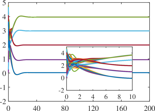
(a) $x_{\operatorname{v}}$

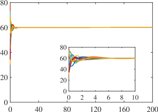
(b) $\lambda_{\operatorname{v}}$

Figure 1: Illustration of the execution of the dynamics (20) to find a data-driven solution of the regression problem (40). Plots (a) and (b) depict the evolution of the primal variables of the distributed optimization problem (12) defined for (40) with $\epsilon=0.05$ (for the sake of simplicity we have not shown the dual variables). The number of agents is $10$ and each agent collects $30$ i.i.d samples of the random variable. The initial condition $(x_{\operatorname{v}}(0),\lambda_{\operatorname{v}}(0))$ is chosen randomly from the set $[0,5]^{50}\times[30,80]^{10}$ and $\nu(0)=\mathbf{0}_{10}$, $\eta(0)=\mathbf{0}_{50}$, and $\xi^{k}(0)=\mathbf{0}_{5}$ for all $k\in[N]$. The primal variables converge to $x_{\operatorname{v}}=\mathbf{1}_{10}\otimes x^{*}$ and $\lambda_{\operatorname{v}}=\lambda^{*}\mathbf{1}_{10}$ with $x^{*}=(0.9460;3.9624;2.9840;1.9878;0.0268)$ and $\lambda^{*}=58.4100$. This is an equilibrium point of $X_{\text{sp}}$ as well as an optimizer of (12). The agents reach consensus early in the execution. Therefore, we only observe $5$ (resp. $1$) curves in the plot of $x_{\operatorname{v}}$ (resp. $\lambda_{\operatorname{v}}$), each corresponding to a component of $x$ (resp. $\lambda$). To depict this consensus clearly, we provided the zoomed part of the initial $10$ seconds for both $x_{\operatorname{v}}$ and $\lambda_{\operatorname{v}}$ plots.

Figure 1 shows the execution of the distributed algorithm (20) that solves this problem. The trajectories converge to an equilibrium of the dynamics (20) whose $(x_{\operatorname{v}},\lambda_{\operatorname{v}})$ component corresponds to an optimizer of (12), consistent with Corollary VII.6. Furthermore, due to the projection operator in the dynamics, trajectories are contained in the set $\mathcal{C}$ given in (39) with $a=1$. Note that if one knows beforehand that $\lambda^{*}\geq a\|(x^{*}_{1:m-1};1)\|^{2}$ for some $a>1$, then one could further restrict the domain of the dynamics.

To evaluate the quality of the obtained solution, we compute the average value of the loss function $f$ for a randomly generated validation dataset consisting of $N_{\mathrm{val}}=10^{4}$ data points $\{(\widehat{w}^{k}_{\mathrm{val}},\widehat{y}^{k}_{\mathrm{val}})\}_{k=1}^{N_{\mathrm{val}}}$. These points are i.i.d with the same distribution as that of the training dataset generated above. Given the obtained solution $(\mathbf{1}_{10}\otimes x^{*},\lambda^{*}\mathbf{1}_{10})$, see Figure 1, we evaluate

$$f_{\mathrm{val}}^{N_{\mathrm{val}}}(x^{*})=\frac{1}{N_{\mathrm{val}}}\sum_{k=1}^{N_{\mathrm{val}}}f(x^{*},\widehat{w}_{\mathrm{val}}^{k},\widehat{y}_{\mathrm{val}}^{k})$$ (41)

and get $f_{\mathrm{val}}^{N_{\mathrm{val}}}(x^{*})=0.3387$. This is the average loss for the solution $x^{*}$ obtained by the agents cooperating with each other, essentially fusing the information of the $300$ data points. Note that each agent individually can also solve a data-driven solution with the samples gathered by it. However, the solution obtained in such a manner, in general, incurs a higher average loss. In the current setup, if agent $1$ solves (10) only with the data available to it (and keeping other parameters equal), then it gets the optimizer as $x^{\mathrm{opt,1}}=(0.8548;3.8933;2.8623;2.1317;0.2227)$. Using the validation dataset, we obtain $f_{\mathrm{val}}^{N_{\mathrm{val}}}(x^{\mathrm{opt,1}})=0.4520$, which is significantly greater than $f_{\mathrm{val}}^{N_{\mathrm{val}}}(x^{*})$. This shows the value of cooperation, that is, fusing the information contained in the data available to different agents leads to an optimizer with better out-of-sample performance. To highlight this fact further, Figure 2 shows the effect of the number of cooperating agents on the average loss incurred by the obtained solution to the data-driven optimization problem. As the plot shows, the improvement in performance due to coordination becomes more prominent as the size of the coordination agents grows.

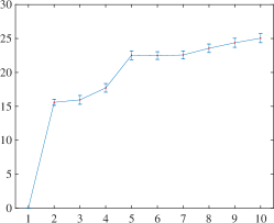
Figure 2: Relative benefit of cooperation versus isolation. The $x$-axis represents the number of agents cooperating in our example. The $y$-axis plots the function $R(i):=\frac{f_{\mathrm{val}}^{N_{\mathrm{val}}}(x^{\mathrm{opt,1}})-f_{\mathrm{val}}^{N_{\mathrm{val}}}(x^{\mathrm{opt,i}})}{f_{\mathrm{val}}^{N_{\mathrm{val}}}(x^{\mathrm{opt,1}})}\times 100\%$. Here, the function $f_{\mathrm{val}}^{N_{\mathrm{val}}}$ is given in (41) and $x^{\mathrm{opt,i}}$ denotes the solution of (10) determined by $i$ cooperating agents. That is, $R(i)$ for each $i\in[n]$ represents the relative decrease in the average loss when $i$ agents cooperate, taking the base case as no cooperation ($i=1$). Thus, as more agents cooperate, the average loss decreases. The error bars represent the standard deviation of $R(i)$ values as we carry out $100$ runs of the simulation, randomly generating different validation data each time.

IX Conclusions

We have considered a cooperative stochastic optimization problem, where a group of agents rely on their individually collected data to collectively determine a data-driven solution with guaranteed out-of-sample performance. Our technical approach has proceeded by first developing a reformulation in the form of a distributed optimization problem, leading us to the identification of an augmented Lagrangian function whose saddle points have a one-to-one correspondence with the primal-dual optimizers. This characterization relies upon certain interchangeability properties between the min and max operators. Our discussion has identified several classes of objective functions for which these properties hold: convex-concave functions, convex-convex functions quadratic in the data, and convex-convex functions associated to least-squares problems. Building on the analytical results, we have designed a distributed saddle-point coordination algorithm where agents share their individual estimates about the solution, not the collected data. We have also formally established the asymptotic convergence of the algorithm to the solution of the cooperative stochastic optimization problem. Future work will explore the characterization of the algorithm convergence rate, the design of strategies capable of tracking the solution of the stochastic optimization problem when new data becomes available in an online fashion, and the analysis of scenarios with network chance constraints.

References

- [1] A. Cherukuri and J. Cortés, “Data-driven distributed optimization using Wasserstein ambiguity sets,” in Allerton Conf. on Communications, Control and Computing, (Monticello, IL), pp. 38–44, 2017.
- [2] A. Shapiro, D. Dentcheva, and A. Ruszczyński, Lectures on stochastic programming. Philadelphia, PA: SIAM, 2014.
- [3] P. M. Esfahani and D. Kuhn, “Data-driven distributionally robust optimization using the Wasserstein metric: performance guarantees and tractable reformulations,” Mathematical Programming, vol. 171, no. 1, pp. 115–166, 2018.
- [4] D. Bertsimas, V. Gupta, and N. Kallus, “Robust sample average approximation,” Mathematical Programming, vol. 171, no. 1, pp. 217–282, 2018.
- [5] R. Gao and A. J. Kleywegt, “Distributionally robust stochastic optimization with Wasserstein distance,” 2016. Available at https://arxiv.org/abs/1604.02199.
- [6] F. Luo and S. Mehrotra, “Decomposition algorithm for distributionally robust optimization using Wasserstein metric,” 2017. Available at https://arxiv.org/abs/1704.03920.
- [7] C. Zhao, Data-driven risk-averse stochastic program and renewable energy integration. PhD thesis, University of Florida, 2014.
- [8] J. Blanchet, Y. Kang, and K. Murthy, “Robust Wasserstein profile inference and applications to machine learning,” 2017. Available at https://arxiv.org/abs/1610.05627.
- [9] R. Jiang and Y. Guan, “Data-driven chance constrained stochastic program,” Mathematical Programming, Series A, vol. 158, pp. 291–327, 2016.
- [10] E. Erdoğan and G. Iyengar, “Ambiguous chance constrained problems and robust optimization,” Mathematical Programming, Series B, vol. 107, pp. 37–61, 2006.
- [11] E. Delage and Y. Ye, “Distributionally robust optimization under moment uncertainty with application to data-driven problems,” Operations Research, vol. 58, pp. 595–612, 2010.
- [12] W. Wieseman, D. Kuhn, and M. Sim, “Distributionally robust convex optimization,” Operations Research, vol. 62, no. 6, pp. 1358–1376, 2014.
- [13] Z. Hu and L. J. Hong, “Kullback-leibler divergence constrained distributionally robust optimization,” 2013. Available at Optimization Online.
- [14] J. Blanchet and K. Murthy, “Quantifying distributional model risk via optimal transport,” 2017. Available at https://arxiv.org/abs/1604.01446.
- [15] D. P. Bertsekas and J. N. Tsitsiklis, Parallel and Distributed Computation: Numerical Methods. Athena Scientific, 1997.
- [16] M. G. Rabbat and R. D. Nowak, “Quantized incremental algorithms for distributed optimization,” IEEE Journal on Selected Areas in Communications, vol. 23, no. 4, pp. 798–808, 2005.
- [17] P. Wan and M. D. Lemmon, “Event-triggered distributed optimization in sensor networks,” in Symposium on Information Processing of Sensor Networks, (San Francisco, CA), pp. 49–60, 2009.
- [18] A. Nedic and A. Ozdaglar, “Distributed subgradient methods for multi-agent optimization,” IEEE Transactions on Automatic Control, vol. 54, no. 1, pp. 48–61, 2009.
- [19] B. Johansson, M. Rabi, and M. Johansson, “A randomized incremental subgradient method for distributed optimization in networked systems,” SIAM Journal on Control and Optimization, vol. 20, no. 3, pp. 1157–1170, 2009.
- [20] M. Zhu and S. Martínez, “On distributed convex optimization under inequality and equality constraints,” IEEE Transactions on Automatic Control, vol. 57, no. 1, pp. 151–164, 2012.
- [21] J. Wang and N. Elia, “A control perspective for centralized and distributed convex optimization,” in IEEE Conf. on Decision and Control, (Orlando, Florida), pp. 3800–3805, 2011.
- [22] A. Nedić, “Distributed optimization,” in Encyclopedia of Systems and Control (J. Baillieul and T. Samad, eds.), New York: Springer, 2015.
- [23] B. Gharesifard and J. Cortés, “Distributed continuous-time convex optimization on weight-balanced digraphs,” IEEE Transactions on Automatic Control, vol. 59, no. 3, pp. 781–786, 2014.
- [24] T. H. de Mello and G. Bayraksan, “Monte Carlo sampling-based methods for stochastic optimization,” Surveys in Operations Research and Management Science, vol. 19, no. 1, pp. 56–85, 2014.
- [25] A. Nemirovski, A. Juditsky, G. Lan, and A. Shapiro, “Robust stochastic approximation approach to stochastic programming,” SIAM Journal on Optimization, vol. 19, no. 4, pp. 1574–1609, 2009.
- [26] F. Bullo, J. Cortés, and S. Martínez, Distributed Control of Robotic Networks. Applied Mathematics Series, Princeton University Press, 2009. Electronically available at http://coordinationbook.info.
- [27] R. T. Rockafellar, Convex Analysis. Princeton Landmarks in Mathematics and Physics, Princeton, NJ: Princeton University Press, 1997. Reprint of 1970 edition.
- [28] A. Bacciotti and F. Ceragioli, “Nonpathological Lyapunov functions and discontinuous Caratheodory systems,” Automatica, vol. 42, no. 3, pp. 453–458, 2006.
- [29] J. Cortés, “Discontinuous dynamical systems - a tutorial on solutions, nonsmooth analysis, and stability,” IEEE Control Systems, vol. 28, no. 3, pp. 36–73, 2008.
- [30] A. Nagurney and D. Zhang, Projected Dynamical Systems and Variational Inequalities with Applications, vol. 2 of International Series in Operations Research and Management Science. Dordrecht, The Netherlands: Kluwer Academic Publishers, 1996.
- [31] S. Lang, Real and Functional Analysis. New York: Springer, 3 ed., 1993.
- [32] F. H. Clarke, Optimization and Nonsmooth Analysis. Canadian Mathematical Society Series of Monographs and Advanced Texts, Wiley, 1983.
- [33] A. E. Ozdaglar and P. Tseng, “Existence of global minima for constrained optimization,” Journal of Optimization Theory & Applications, vol. 128, no. 3, pp. 523–546, 2006.
- [34] R. Gao, X. Chen, and A. J. Kleywegt, “Distributional robustness and regularization in statistical learning,” 2017. Available at https://arxiv.org/abs/1712.06050.
- [35] A. Cherukuri, B. Gharesifard, and J. Cortés, “Saddle-point dynamics: conditions for asymptotic stability of saddle points,” SIAM Journal on Control and Optimization, vol. 55, no. 1, pp. 486–511, 2017.
- [36] X. L. Sun, D. Li, and K. I. M. Mckinnon, “On saddle points of augmented Lagrangians for constrained nonconvex optimization,” SIAM Journal on Optimization, vol. 15, no. 4, pp. 1128–1146, 2005.
- [37] A. Cherukuri, E. Mallada, and J. Cortés, “Asymptotic convergence of constrained primal-dual dynamics,” Systems & Control Letters, vol. 87, pp. 10–15, 2016.
- [38] A. Cherukuri, E. Mallada, S. H. Low, and J. Cortés, “The role of convexity in saddle-point dynamics: Lyapunov function and robustness,” IEEE Transactions on Automatic Control, vol. 63, no. 8, pp. 2449–2464, 2018.
- [39] S. P. Bhat and D. S. Bernstein, “Nontangency-based Lyapunov tests for convergence and stability in systems having a continuum of equilibria,” SIAM Journal on Control and Optimization, vol. 42, no. 5, pp. 1745–1775, 2003.
- [40] R. Goebel, “Stability and robustness for saddle-point dynamics through monotone mappings,” Systems & Control Letters, vol. 108, pp. 16–22, 2017.
- [41] D. Richert and J. Cortés, “Distributed linear programming with event-triggered communication,” SIAM Journal on Control and Optimization, vol. 54, no. 3, pp. 1769–1797, 2016.
- [42] S. S. Kia, J. Cortés, and S. Martínez, “Distributed convex optimization via continuous-time coordination algorithms with discrete-time communication,” Automatica, vol. 55, pp. 254–264, 2015.
- [43] D. Mateos-Núñez and J. Cortés, “Noise-to-state exponentially stable distributed convex optimization on weight-balanced digraphs,” SIAM Journal on Control and Optimization, vol. 54, no. 1, pp. 266–290, 2016.
- [44] A. Nedić and A. Ozdaglar, “Subgradient methods for saddle-point problems,” Journal of Optimization Theory & Applications, vol. 142, no. 1, pp. 205–228, 2009.
- [45] D. Mateos-Núñez and J. Cortés, “Distributed saddle-point subgradient algorithms with Laplacian averaging,” IEEE Transactions on Automatic Control, vol. 62, no. 6, pp. 2720–2735, 2017.
- [46] B. Schölkopf and A. J. Smola, Learning with kernels. Cambridge, MA: MIT Press, 2002.