The $Gaia$-ESO Survey: Lithium enrichment histories
of the Galactic thick and thin disc

Lithium abundance in most of the warm metal-poor main sequence stars shows a constant plateau (A(Li) $\sim$ 2.2 dex) and then the upper envelope of the lithium vs. metallicity distribution increases as we approach solar metallicity. Meteorites, which carry information about the chemical composition of the interstellar medium at the solar system formation time, show a lithium abundance A(Li)$\sim$ 3.26 dex. This pattern reflects the Li enrichment history of the interstellar medium during the Galaxy lifetime. After the initial Li production in Big Bang Nucleosynthesis, the sources of the enrichment include AGB stars, low-mass red giants, novae, type II supernovae, and Galactic cosmic rays. The total amount of enriched Li is sensitive to the relative contribution of these sources. Thus different Li enrichment histories are expected in the Galactic thick and thin disc. We investigate the main sequence stars observed with UVES in $Gaia$-ESO Survey iDR4 catalog and find a Li- [$\alpha$/Fe] anticorrelation independent of [Fe/H] , T_eff , and $\log(g)$ . Since in stellar evolution different $\alpha$ enhancements at the same metallicity do not lead to a measurable Li abundance change, the anticorrelation indicates that more Li is produced during the Galactic thin disc phase than during the Galactic thick disc phase. We also find a correlation between the abundance of Li and s-process elements Ba and Y, and they both decrease above the solar metallicity, which can be explained in the framework of the adopted Galactic chemical evolution models.

1 Introduction

The evolution of lithium (⁷Li) in the Galaxy is a critical and not well understood issue, because of the many unknowns that still affect the proposed production and destruction channels of this element. Most of the metal-poor ($-$2.4 $\lesssim$ [Fe/H] $\lesssim-$1.4), warm (5700 K $\lesssim T_{\mathrm{eff}}\lesssim$ 6800 K) Galactic halo dwarfs are known to share a very similar ⁷Li abundance, the so-called ”Spite plateau” (A(Li) $\simeq$ 2.05 – 2.2 dex, Spite & Spite, 1982; Bonifacio & Molaro, 1997; Asplund et al., 2006; Bonifacio et al., 2007), which for a long time has been thought to represent the primordial Li abundance produced in the Big Bang Nucleosynthesis. However, Standard Big Bang Nucleosynthesis (SBBN) predicts that the primordial Li abundance is mainly determined by the primordial baryon-to-photon ratio which can be derived from the acoustic oscillations of the cosmic microwave background (CMB), and the baryon-to-photon ratio obtained by the Planck satellite data leads to A(Li) = 2.66 – 2.73 dex (Coc et al., 2014), i.e. the SBBN predicted primordial Li abundance exceeds the stellar observationally inferred value by a factor of almost three. Furthermore, the Spite plateau is not constant, but bends down for extremely metal-poor stars ([Fe/H] $\lessapprox-$2.8 dex, e.g. Sbordone et al., 2010; Melendez et al., 2010; Hansen et al., 2014; Bonifacio et al., 2015). The environmental ⁷Li evolution model proposed by Fu et al. (2015) offers a way to reconcile the SBBN theory to the observations of stars on the plateau by considering the pre-main sequence accretion, overshooting, and main sequence diffusion, while also accounting for the drop of ⁷Li abundances in extremely metal-poor stars, but it needs to be studied more and better constrained (for instance, by including the effects of stellar rotation).

As far as the Galactic disc stars are concerned, a large dispersion is seen in the data (see Ramírez et al., 2012; Delgado Mena et al., 2015; Guiglion et al., 2016, for recent works). The observed scatter is due to efficient ⁷Li destruction in stellar interiors (e.g., A_Li = 1.05 dex in the Sun, Grevesse et al., 2007), coupled to non-negligible ⁷Li production on a Galactic scale. The discovery of unevolved stars with high ⁷Li abundances (comparable or higher than those observed in meteorites, A(Li) = 3.26 dex, Lodders et al., 2009), dates to long ago (see e.g. Bonsack & Greenstein, 1960; Herbig, 1965; Wallerstein et al., 1965, for T Tauri, F and G dwarf, and Hyades main-sequence stars, respectively), and it is now commonly interpreted as a signature of ⁷Li enrichment of the interstellar medium (ISM), due to various production processes. Indeed, ⁷Li is synthesized in different astrophysical sites, apart from the Big Bang:

• High-energy processes involving Galactic cosmic rays (GCRs) hitting the ISM atoms contribute to less than 20 – 30 per cent to the meteoritic ⁷Li abundance (Reeves et al., 1970; Meneguzzi et al., 1971; Lemoine et al., 1998; Romano et al., 2001; Prantzos, 2012), so that about 70% of the Solar System ⁷Li must originate from thermonuclear reactions acting in the stellar interiors.

• As first suggested by Domogatskii et al. (1978), the $\nu$-process may lead to the synthesis of ⁷Li in the helium shell of core-collapse supernovae (SNe). However, this mechanism ought to work quite inefficiently at a Galactic level (see discussions in Vangioni-Flam et al., 1996; Romano et al., 1999); furthermore, to the best of our knowledge there is no observational evidence in support of it.

• Observations in both the Milky Way (disc, bulge, halo, Globular Clusters, e.g. Wallerstein & Sneden, 1982; Pilachowski, 1986; Hill & Pasquini, 1999; Kraft et al., 1999; Balachandran et al., 2000; Kumar & Reddy, 2009; Monaco et al., 2011; D’Orazi et al., 2015; Casey et al., 2016; Kirby et al., 2016) and Local Group dwarf galaxies (Domínguez et al., 2004; Kirby et al., 2012) have conclusively shown that a number of Li-rich giants do exist with abundances higher than the standard stellar evolution theory predicts (A(Li)$\sim$ 1.0 dex at the beginning of the Red Giant Branch bump for Pop. II stars around 1 M_⊙(Charbonnel & Zahn, 2007; Fu, 2016), and even lower for more massive stars (Iben, Icko, 1967a, b) ), or even exceeding the SBBN prediction and the meteorites’ value, indicating that the Li in these stars must have been created rather than preserved from destruction. Stars can produce ⁷Li in their late stages of evolution via the Cameron-Fowler mechanism (Cameron & Fowler, 1971), which may work both in intermediate-mass stars on the asymptotic giant branch (AGB) (Sackmann & Boothroyd, 1992) and in low-mass stars on the red giant branch (RGB), under special conditions (Sackmann & Boothroyd, 1999). Abia et al. (1993) conclude that the contribution of carbon stars can reach 30% to the Galactic Li enrichment depending on the mass loss and Li production in the Li-rich AGB stars. However, the detailed mechanism(s) of the Li enrichment in these giant stars is still an open problem, and we lack a clear and unequivocal assessment of the relative contributions of these two stellar contributions to the overall Galactic lithium enrichment: for instance, Romano et al. (2001) and Travaglio et al. (2001) reach opposite conclusions, because of the adoption of different yield sets and different assumptions about the underlying stellar physics (e.g. mixing process, mass loss rate) in their chemical evolution models.

• Another, potentially major source of ⁷Li are nova systems, which are able to produce it when a thermonuclear runaway occurs in the hydrogen envelope of the accreting white dwarf, as proposed long ago by Starrfield et al. (1978). Notwithstanding the considerable observational efforts, a direct detection of ⁷Li during a nova outburst remained elusive until the very recent detection of the blueshifted Li I $\lambda$ 6708 Å line in the spectrum of the nova V1369 Cen by Izzo et al. (2015). Based on the intensity of the absorption line and on current estimates of the Galactic nova rate, Izzo et al. (2015) estimate that novae might be able to explain most of the enriched lithium observed in the young stellar populations. Further support in favour of a high production of ⁷Li during nova outbursts comes from the detection of highly enriched ⁷Be (later decaying to ⁷Li) in the ejecta of novae V339 Del, V2944 Oph, and V5668 Sgr by Tajitsu et al. (2015) and Tajitsu et al. (2016), respectively (see also Molaro et al., 2016).

In this paper, we investigate the lithium content and enrichment history in (mostly) thin and thick disc stars in the Milky Way, as well as its relationships with the abundances of selected $\alpha$ and $s$-process elements. To do so, we take advantage of UVES spectra analysed by the $Gaia$-ESO consortium for 1399 main sequence stars. Furthermore, we use an updated version of the model presented by Romano et al. (1999, 2001), that takes all of the above-mentioned sources of lithium into account (see also Izzo et al., 2015), to discuss our ⁷Li measurements. In particular, we show that, in principle, in the framework of such a model it is possible to offer an explanation for the observed peculiar trend of decreasing ⁷Li for super-solar metallicity stars (Delgado Mena et al., 2015; Guiglion et al., 2016), if it is real.

The paper is organised as follows. In section  2 we describe the observations, data analysis, and sample selection. The main results are presented in section  3, including the trends of Li abundances in thin and thick disc stars, also in relation with the $\alpha$ and s-process elements behaviours. In section 4 we discuss the Galactic chemical evolution of Li. The conclusions and a final summary are given in section  5.

2 $Gaia$-ESO Survey observations and data analysis

The $Gaia$-ESO Survey (GES hereafter, Gilmore et al., 2012; Randich et al., 2013) is a large, public, high-resolution spectroscopic survey using the FLAMES facility at ESO Very Large Telescope (VLT), i.e. it simultaneously employs the UVES and GIRAFFE spectrographs (Dekker et al., 2000; Pasquini et al., 2000). GES is intended to complement the $Gaia$ astrometric and photometric data of exquisite precision (Gaia Collaboration et al., 2016) with radial velocities and detailed chemistry for about $10^{5}$ stars of all major Galactic populations and about 70 open clusters (which will not be considered further in the paper since the purpose of this paper is to investigate the chemical evolution of the field stars.)

To study the Milky Way (MW) field population, GES uses mostly the medium-resolution spectrograph GIRAFFE with two setups (HR10, HR21). However, GES also observes MW field stars with UVES and a setup centred at 580nm ($\lambda=480-680$ nm, $R\sim 47,000$) and is collecting high-resolution, high signal-to-noise (SNR) spectra of a few thousand FG-type stars in the solar neighbourhood (within about 2 kpc from the Sun). This sample includes mainly disc stars of all ages and metallicities, plus a small fraction of local halo stars, and it is intended to produce a detailed chemical and kinematical characterization, to fully complement the results of the $Gaia$ mission, which achieve their maximum precision within this distance limit.

The detailed description of the MW sample selection is presented in Stonkutė et al. (2016). In brief, the UVES observations are made in parallel with the GIRAFFE ones and their position and exposure time are dictated by the latter. The 2MASS infrared photometry (Skrutskie et al., 2006) was used to select dwarfs and main sequence turn-off stars of FG spectral type, with a limiting magnitude of $J_{2MASS}=14$ and a narrow colour range. The selection takes into account also the effects of interstellar extinction, estimated through the reddening maps of Schlegel et al. (1998) Though some remaining uncertainties still affect the evolutionary phases of the stars, the majority of the observed targets turn out to be dwarf stars, as we will show later in Sec. 2.1.

Multiple analysis pipelines are used by GES to produce stellar parameters and chemical abundances. The working group (WG) that takes care of FGK-type UVES spectra is WG11, split in different nodes producing independent results (Smiljanic et al., 2014). The UVES spectrum reduction is centralized (see Sacco et al., 2014, for a description) and each node is provided with 1-d, wavelength calibrated, and sky subtracted spectra. Up to 11 nodes produced UVES results for iDR4, they have in common the stellar atmospheres (1-d MARCS, Gustafsson et al., 2008), the line list (Ruffoni et al., 2014; Heiter et al., 2015), and the solar reference abundances (Grevesse et al., 2007), see Pancino et al. (2017) for the calibration strategy. The node results are homogenized by WG11 and subsequently by WG15 (see for instance Casey et al., 2016, for more details), producing the recommended parameters and chemical abundances released first internally and then to the public. We use here the internal data release 4 (iDR4) which contains 54,490 stars observed up to the end of June 2014 (i.e., 30 months); the public version, released after a further validation process, can be accessed through the ESO Phase 3 webpage (http://www.eso.org/qi/).

2.1 Sample selection

To investigate the Galactic lithium enrichment history we select well-measured main sequence field stars with UVES spectra from the GES iDR4 catalog. In our selection 1884 UVES stars are marked as field stars, including those of the Galactic disc and halo designated as Milky Way ($GE\_MW$) fields, standard CoRoT ($GE\_SD\_CR$) field, standard radial velocity ($GE\_SD\_RV$) field, and stars to the Galactic Bulge direction ($GE\_MW\_BL$). Note that these classifications are also used in the public GES data releases. We set the surface gravity $\log(g)$ =3.7 dex as the criterion to separate the dwarf and giant stars, Fig. 1 illustrates the division. The dwarfs largely outnumber the interloping giants (in our field UVES sample we have 1524 dwarfs and 360 giants, respectively), this indicates that the GES target selection was successful.

We exclude the evolved giant stars in this study because their Li abundances are altered by internal mixing processes and do not reflect anymore the Galactic Li enrichment history. When stars experience their first dredge-up after leaving the main sequence the surface convective zone deepens and brings materials from the hot interior to the stellar surface. Lithium, which is easily destroyed at several million Kelvin, has its abundance significantly decreased at this stage because of both dilution and destruction. In fact, we also use this Li abundance drop to ensure that our dwarf-giant separation at $\log(g)$ =3.7 is reliable (see the left panel of Fig. 1). We note that there are several giants in this figure that do not follow the A(Li)-$\log(g)$ trend, these stars have already been discussed by Casey et al. (2016) who report on the ”Li-rich giant problem” using GES data. Compared to the giant stars, main sequence stars with the same stellar mass have a much thinner surface convective zone that could save Li from destruction. In this paper we focus on these main sequence stars with $\log(g)$ $\geq$ 3.7 dex.

However, for main sequence star another long-term stellar process, microscopic diffusion, could also lead to a depletion of the surface elements as the star ages (see e.g. Richard et al., 2002; Korn et al., 2007; Xiong & Deng, 2009; Nordlander et al., 2012; Fu et al., 2015; Dotter et al., 2017). To ensure that different ages of our sample stars do not introduce a significant dispersion in Li abundance, we check the pure effect of microscopic diffusion using the stellar model code  PARSEC (V1.2s, Bressan et al., 2012). Three kinds of microscopic diffusion, including pressure diffusion, temperature diffusion, and concentration diffusion, as described in Thoul et al. (1994), are considered. To simulate the pure effect of microscopic diffusion, neither extra mixing (e.g. envelope overshooting) nor pre-main sequence accretion is applied in the models. In Fig. 2 three solar metallicity stars with different masses are shown as examples. Starting from the meteorites’ Li abundance, the main Li destruction in these stars occurs early in stellar life (see also Chen et al., 2001). During their main sequence phase Li abundances (solid lines) decrease $\sim$0.2 dex. Their temperatures at the bottom of the surface convective zone ($T_{bot}$, dotted lines), which is an indicator of the rate of Li burning, are so low (1.3$\sim$2.5 $\times 10^{6}$ K) that even 7-10 Gyr of evolution can not lead to a notable destruction. Thus Li depletion from nuclear reaction is negligible in these stars during the main sequence phase, the main depletion comes from the microscopic diffusion. Microscopic diffusion takes 7-10 Gyr to decrease $\sim$ 0.2 dex of the surface Li abundance, which is the typical Li measurement uncertainty of our sample. If extra mixing, which slows the diffusion (Xiong & Deng, 2009), is considered, the depletion time will be even longer. Therefore, even a 7-10 Gyr age difference of the Galactic field stars will not affect our investigation. For stars with lower mass thus deeper surface convective zone (e.g. M=0.90M_⊙  star in Fig. 2), their Li depletion can be traced by T_eff , we will discuss it in detail in Sec.  3.

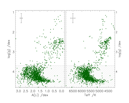
Figure 1: Field stars in GES iDR4 catalog with UVES observations. The left panel displays the Li content (LTE) against $\log(g)$ , and the right panel shows $\log(g)$ , as an indicator of the evolutionary phase, against effective temperature (T_eff ). We consider stars with $\log(g)$ $\geq 3.7$ dex, namely those falling in the shaded areas, as main sequence stars. The median values of the parameter error are displayed in the left upper corner of each panel.

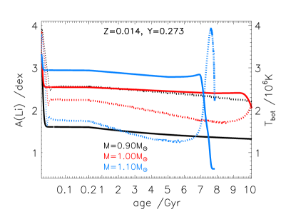
Figure 2: Pure effect of microscopic diffusion on Li abundance during the first 10 Gyr from stellar model  PARSEC . Neither envelope overshooting nor pre-main sequence accretion is applied. Li abundances (solid lines) and the temperature at the bottom of surface convective zone ($T_{bot}$, dotted lines) are displayed as a function of stellar age. Different colors indicate different stellar mass as indicated in the legend.

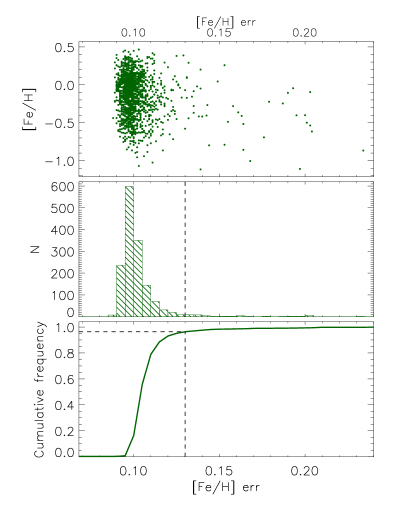
Figure 3: Distribution of [Fe/H] error for main sequence field UVES stars in GES iDR4 catalog. The upper panel displays the relation of [Fe/H] and [Fe/H] error, while the center and lower panel show the histogram and cumulative frequency of [Fe/H] error, respectively. Ninety-five percent of stars lie in the interval smaller than 0.13 dex (vertical dashed lines in the last two panels).

We then exclude stars with large [Fe/H] errors. Fig. 3 shows the distribution of [Fe/H] error for the 1524 main sequence field UVES stars; those with [Fe/H] error ¡ 0.13 dex (95% of the sample) are selected as ”well-measured” objects. Some of the well-measured stars are members of multiple stellar system, or have emission lines in their spectra. Since multiple stellar system members carve up their initial Li (e.g. in binary stars the primary one has higher Li abundance, González Hernández et al., 2008; Aoki et al., 2012; Fu et al., 2015) and the emission lines are likely from pre-main sequence stars which may undergo a Li-depletion, we remove these stars from our sample to avoid confusion. This reduces the sample to 1432 objects. In GES iDR4, 1097 of them are labeled as stars with Li upper limits, and 335 as true measurements. We double check the spectra of stars with labeled Li measurements and mark 302 of them as high quality spectra around the Li resonance line. In our final sample we thus have 1399 well-measured UVES main sequence field stars sorted into two categories: i) labeled Li upper limits (1097 stars, with signal-to-noise ratio (SNR) ranging in 12 - 259 and median SNR=63), and ii) checked Li measurements (302 stars, SNR from 18 to 319, and median SNR=83).

3 Results

The abundance analysis of Li in GES iDR4 is based on the local thermodynamic equilibrium (LTE) assumption, however in reality the line formation in stellar atmosphere is a more complex process, and non-local thermodynamic equilibrium (NLTE) effect should be accounted for. We apply the NLTE corrections to the Li I $\lambda=6708$ Å line using the correction grid from Lind et al. (2009). Fig. 4 displays the correction departures ($A_{Li}^{NLTE}$-$A_{Li}^{LTE}$) as a function of each parameter ($A_{Li}^{LTE}$, T_eff , [Fe/H], $\log(g)$ , and micro-turbulence $\xi$), respectively. We calculate also the NLTE correction uncertainties introduced by the errors of these parameters. The median values of the uncertainties are $\sim 0.02-0.035$ dex from each parameter, which are negligible. The overall NLTE corrections, as seen from Fig. 4, are not significant for stars in our sample, even the largest departure is less than or equal to the value of the typical Li abundance error ($\sim 0.2$ dex) in LTE. Table  2 lists the LTE and NLTE results, together with other chemical abundances and the stellar parameters that we use in this study. Hereafter we use A_Li to represent A${}_{\mathrm{Li}}^{NLTE}$ .

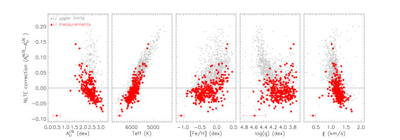
Figure 4: NLTE Li abundances corrections verses various parameters. The filled red squares are stars with checked Li measurements (302 stars), and grey dots represent those labeled with Li upper limits in GES iDR4 catalog (1097 stars). The median error of each parameter is displayed in the left lower corner of each panel.

Table 1: Stellar parameters, the selected chemical abundances, and their corresponding uncertainties of stars in our final sample.

cname	object	$A_{Li}^{LTE}$	A${}_{\mathrm{Li}}^{NLTE}$	category	[$\alpha$/Fe]	[Fe/H]	$\log(g)$	Teff	[Ba II/Fe]	[Y II/Fe]
18342649-2707171	100001	2.63 $\pm$ 0.21	2.63	meas.	0.05$\pm$ 0.13	0.11 $\pm$ 0.10	4.17 $\pm$ 0.23	6049 $\pm$ 114	-0.09$\pm$ 0.17	-0.11$\pm$ 0.18
18253560-2525493	100003	2.64 $\pm$ 0.22	2.61	meas.	-0.06$\pm$ 0.12	-0.19 $\pm$ 0.10	4.24 $\pm$ 0.23	5958 $\pm$ 112	0.16$\pm$ 0.17	-0.13 $\pm$ 0.18
…	…	…	…	…	…	…	…	…	…	…
18225412-3410286	100024	0.49	0.62	La.upper	0.30 $\pm$ 0.14	-0.45 $\pm$ 0.11	4.22 $\pm$ 0.3	4858 $\pm$ 139	-0.37 $\pm$ 0.18	0.42 $\pm$ 0.18
19241832+0057159	100733229	1.22	1.31	La.upper	0.11 $\pm$ 0.13	0.13 $\pm$ 0.10	4.38 $\pm$ 0.22	5483 $\pm$ 119	-0.17 $\pm$ 0.18	-0.12 $\pm$ 0.17
…	…	…	…	…	…	…	…	…	…	…

In Fig. 5 we present the general behaviours of A_Li against T_eff , $\log(g)$ , and [Fe/H], respectively. Cooler stars show lower Li abundances as expected (see the left panel) because they have a deeper surface convective zone which burns Li. The coolest stars with Li upper limits are also those that have larger $\log(g)$ (see the central panel). They are lower main sequence stars with small stellar mass since $\log(g)$ is an indicator of the evolutionary phase. The upper envelope of the Li evolution with [Fe/H] (see the right panel of Fig. 5) is traditionally believed to reflect the Li enrichment history of the Galactic ISM, taking [Fe/H] as an index of the total metallicity (see Abia et al., 1998; Romano et al., 1999, 2001; Travaglio et al., 2001; Prantzos, 2012).

In the following sections we combine our Li abundances with  [$\alpha$/Fe] ,  [Ba/Fe] , and  [Y/Fe] ratios to shed new light on the Li enrichment histories of different Galactic disc components.

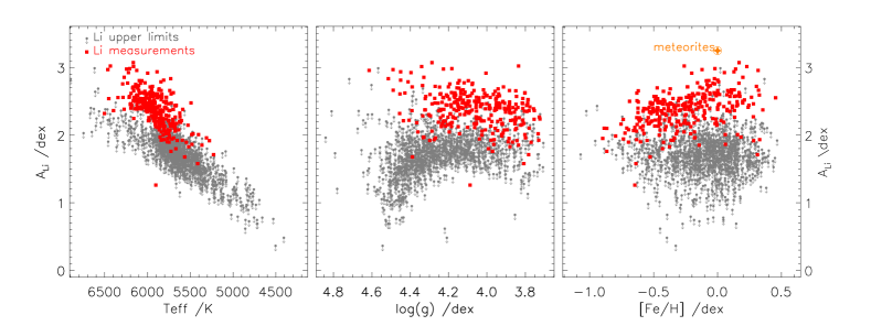
Figure 5: NLTE Li abundance for stars in our final sample as a function of T_eff (left), $\log(g)$ (center), and [Fe/H] (right), respectively. In all three panels, filled red squares are the stars with checked Li measurements (302 stars), and grey dots represent those labeled with Li upper limits in GES iDR4 catalog (1097 stars). The Li abundance of meteorites is also marked in the right panel.

3.1 Distinction between the Galactic thick and thin discs

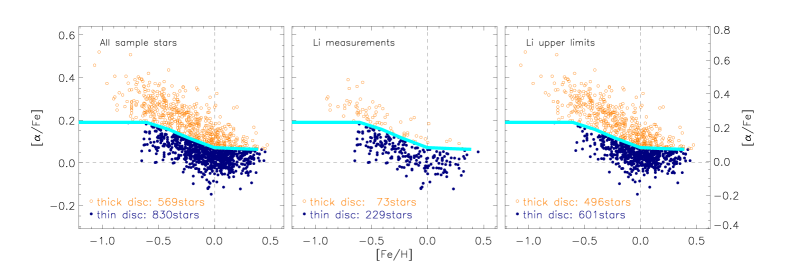
Figure 6: Tentative separation between thick and thin discs in the  [$\alpha$/Fe] -[Fe/H] plane for all sample stars (left panel), stars with Li measurements (central panel), and stars with Li upper limits (right panel). In all panels the vertical and horizontal dashed lines indicate solar values. Filled blue dots represent the Galactic thin disc stars while open orange circles are the thick disc objects. The cyan line shows the division proposed by (Adibekyan et al., 2012).

A precise determination of the Galactic thick and thin disc membership requires a detailed knowledge of the space motions, which are calculated from the stellar distances, proper motions and radial velocities. Unfortunately only nine stars in our sample have this information from $Gaia$ DR1 TGAS catalog (Michalik et al., 2015; Gaia Collaboration et al., 2016). We are looking forward to Gaia DR2, which will be released in spring 2018 and will provide the five-parameter astrometric solutions and help us to draw a precise map of the thick and thin discs for almost the entire $Gaia$ catalog.

The abundance of $\alpha$ elements relative to iron ( [$\alpha$/Fe] ) are often used to chemically separate the Galactic thick disc from thin disc stars when the space motion information is lacking (e.g. Fuhrmann, 1998; Gratton et al., 2000; Reddy et al., 2003; Venn et al., 2004; Bensby et al., 2005; Rojas-Arriagada et al., 2017). The $\alpha$ elements (O, Ne, Mg, Si, S, Ar, Ca, and Ti) are mostly produced by core collapse SNe (mainly Type II SNe) on short time scales, while iron is also synthesized in Type Ia SNe on longer time scales (after at least one white dwarf has been formed). Stars formed shortly after the ISM has been enriched by SNe II have enhanced  [$\alpha$/Fe] ratios, while those formed sometime after SNe Ia have contributed most of Fe have higher iron abundances and lower  [$\alpha$/Fe] ratios. Thus the  [$\alpha$/Fe] ratio is a cosmic-clock, or better, it echoes the formation history (see e.g. Tinsley, 1979; Matteucci & Greggio, 1986; Haywood et al., 2013, and the references therein). The Galactic thick disc stars usually have lower [Fe/H] values and higher  [$\alpha$/Fe] , while most of the thin disc stars tend to have higher iron abundance and lower  [$\alpha$/Fe] values. However the criterion adopted for separation differs in different works.

We define  [$\alpha$/Fe] ratios for the stars in our sample, taking into account four $\alpha$ elements (Mg, Ca, Si, and Ti):

$$n(\alpha)=n(\mathrm{Mg\leavevmode\nobreak\ I})+n(\mathrm{Ca\leavevmode\nobreak\ I})+n(\mathrm{Si\leavevmode\nobreak\ I})+n(\mathrm{Ti\leavevmode\nobreak\ I})+n(\mathrm{Ti\leavevmode\nobreak\ II})$$ (1)

$$$\leavevmode\nobreak\ [$\alpha$/Fe]\leavevmode\nobreak\ $=\mathrm{log}(\frac{n(\alpha)}{n(\mathrm{Fe})})_{\ast}-\mathrm{log}(\frac{n(\alpha)}{n(\mathrm{Fe})})_{\odot}$$ (2)

The other elements (and isotopes) are not included because they are not measured in all our sample stars. By taking into account the measurement uncertainties of the six parameters in Equation  1 and  2 (A(Mg I), A(Si), A(Ca I), A(Ti I), A(Ti II), and [Fe/H] ), we derive the mean value of  [$\alpha$/Fe] and its corresponding 1 $\sigma$ uncertainty using the Markov chain Monte Carlo (MCMC) code emcee (Foreman-Mackey et al., 2013). After a burn-in phase of 100 steps to ensure that the chains have converged, we performed 150 MCMC steps for each star. The final results are listed in Table 2.

Here we perform a tentative separation based on  [$\alpha$/Fe] . We adopt a separation method similar to Recio-Blanco et al. (2014) and Mikolaitis et al. (2014) that divides the sample stars into several [Fe/H] ([M/H] in the case of Recio-Blanco et al., 2014; Mikolaitis et al., 2014) bins and finds the possible  [$\alpha$/Fe] demarcation between the thick and thin discs in each interval. Our resulting tentative division is consistent with the separation proposed by Adibekyan et al. (2012) who separate the high- and low-$\alpha$ stars with very high resolution and high S/N data. In Fig. 6 we show the separation for all sample stars, the division for stars with Li measurements and those with Li upper limits are also displayed. There are 569 stars in our sample possibly belonging to the thick disc (73 of them have Li measurements and 496 are stars with Li upper limits) and 830 stars that are likely thin disc members (229 stars are from the category of Li measurements and 601 stars have Li upper limits). Our tentative separation is essentially similar to the divisions adopted for slightly more metal-poor stars in GES data by Recio-Blanco et al. (2014); Mikolaitis et al. (2014) in the  [$\alpha$/Fe] -[M/H] and [Mg/M]-[M/H] planes. We choose not to adopt that because they are based on GIRAFFE spectra and a previous data release.

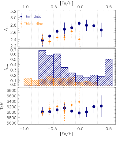
Figure 7: Stars with enriched Li (A_Li $>2.2$ dex). $Upper\leavevmode\nobreak\ panel:$ Error-weighted mean A_Li values of the six stars with the highest Li abundance in each [Fe/H] bin, the standard deviation of their A_Li values is considered as the uncertainty. Blue filled dots represent the thin disc and the orange stars indicate the thick disc. The symbols are displayed when there are more than six Li-enriched thin/thick stars in the bin. $Middle\leavevmode\nobreak\ panel:$ Fractions of Li-enriched stars ($f_{A(Li)>2.2}$) in each [Fe/H] interval for thin disc stars (blue-shades histogram) and thick disc stars (orange-shaded histogram). $Lower\leavevmode\nobreak\ panel:$ Error-weighted mean T_eff values of the six stars with the highest Li abundance in each [Fe/H] bin, the standard deviation of their T_eff values is considered as the uncertainty. Symbols are the same as in the upper panel.

Fig. 7 shows the behaviour of Li enrichment in the two discs, when our sample stars are divided according to the criterion outlined above. All stars with A_Li $>2.2$ dex (the Spite Plateau value) are Li-enriched compared to Pop. II stars. Since we are not able to precisely disentangle thick from thin disc stars in our sample without the space motion information, we can not simply select the highest A_Li as the initial Li value. Therefore, we adopt the method used in Lambert & Reddy (2004); Delgado Mena et al. (2015); Guiglion et al. (2016) that selects the six stars with the highest A_Li in each [Fe/H] bin and calculates their mean A_Li values (weighted by the reciprocal of Li abundance errors in LTE) to track the trend of Li enrichment, the standard deviations of their A_Li is considered the corresponding uncertainty. In the upper panel of Fig. 7 the blue filled dots and the orange stars display these trends for the Galactic thin disc and thick disc, respectively. Our Li trend of thin disc stars is systematically lower than the one proposed by Guiglion et al. (2016), while is compatible with the overall trend of Delgado Mena et al. (2015). This may be because of sample selection effects. Strictly speaking, the trends of main sequence mean A_Li is a lower limit to the real Li evolution in the thin and thick disc, respectively. Some depletion (although perhaps little) has had to happen in both groups of stars. The fraction of the Li-enriched stars in each [Fe/H] interval represents the overall level of Li enrichment. In the middle panel of Fig. 7 we present the fraction of Li-enriched stars in the thin (blue histogram) and thick (orange histogram) discs. The thin disc has much higher Li-enriched star fractions compared to the thick disc. We perform a K-S test to compare the two distributions, the maximum deviation between the cumulative distribution of the two histograms is D=0.75, and the significance level of the K-S statistic is 0.0009. As mentioned in Sec. 2.1, T_eff is a key parameter to trace the stellar Li destruction (stars with lower T_eff have lower A_Li ). In order to investigate whether thick disc stars have experienced a stronger Li destruction than the thin disc stars, we compare the mean T_eff (weighted by the reciprocal of T_eff errors) of the six stars with highest A_Li in each [Fe/H] bin, and take their T_eff standard deviation as the uncertainty, the results are displayed in the lower panel of Fig. 7. It becomes apparent that the thick disc stars do not show a lower T_eff compared to the thin disc stars, in some of the [Fe/H] bins they even have higher T_eff than the thin disc ones though their A_Li is lower as shown in the upper panel of the figure. As seen in all the three panels of Fig. 7, we conclude that the Galactic thin disc has higher A_Li and higher overall level of Li enrichment than the thick disc, the Li trend difference between the thick and thin discs is not due to the stellar destruction, but reflects different initial Li abundances of the two discs.

3.2 Li- [$\alpha$/Fe] anticorrelation

In addition to the tentative thick/thin disc separation, we investigate the relation between A_Li and  [$\alpha$/Fe] , especially for stars with actual Li measurements, in order to gain a deeper insight into the Li enrichment histories of the Galactic thick and thin disc.

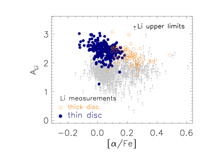
Figure 8: NLTE Li abundance verses  [$\alpha$/Fe] . Stars with Li measurements are separated as thin (filled blue dots) and thick (open orange circles) disc stars, as the same as in the middle panel of Fig. 6. The grey dots represent sample stars with Li upper limits.

In Fig 8 we display the overall relation between A_Li and  [$\alpha$/Fe] . A Li- [$\alpha$/Fe] anticorrelation is clearly seen in this figure and is highly statistically significant (its Pearson’s correlation for stars with Li measurements has confidence level ¿ 99%). However one can not ignore that as [Fe/H] increases, A_Li rises (see the right panel of Fig. 5) while  [$\alpha$/Fe] decreases (see Fig. 6). To eliminate the [Fe/H] evolutionary effect in the Li- [$\alpha$/Fe] anticorrelation, one should compare stars with similar [Fe/H] values. For this purpose we present A_Li as a function of  [$\alpha$/Fe] in different [Fe/H] bins in Fig 9. The bin size is 0.26 dex, which is twice the maximum error on [Fe/H] for our sample stars. To avoid the bin selection bias, 0.13 dex is overlapped between the adjacent [Fe/H] bins. We calculate the mean values of Pearson’s correlation coefficient ($R_{0}(P)$) and its significance level $P_{0}$ between A_Li and  [$\alpha$/Fe] in each [Fe/H] bin. We also derive the possibility of the anticorrelation in each bin taking into account the abundance uncertainties. In this case, Li abundance error in LTE measurement is considered as the uncertainty of NLTE results, and a Bayesian linear regression method described in Kelly (2007) is performed. If the number of stars in the bin is greater than 10, then the Markov chains will be created using the Gibbs sampler, otherwise the Metropolis-Hastings algorithm is used. Negative value of the linear regression slope $\beta$ means anticorrelation. For each [Fe/H] bin, we calculate the possibility of an anticorrelation ($\beta$¡0) of Li- [$\alpha$/Fe] , and find that the possibility is $\gtrsim 68\%\leavevmode\nobreak\ (1\sigma)$ for half of them, with a corresponding $1-2\sigma$ significance of P ¡ 0.05 (i.e. the confidence interval is greater than 95%). This means that, at similar [Fe/H] , A_Li is very likely anti correlated with  [$\alpha$/Fe] for field stars.

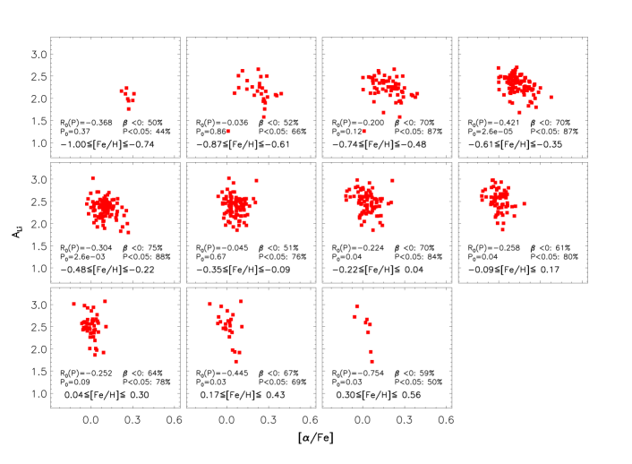
Figure 9: NLTE Li abundance as a function of  [$\alpha$/Fe] in each [Fe/H] bin for our sample stars with Li measurements. The range of [Fe/H] is specified in each plot. The [Fe/H] bin size is 0.26 dex. In each bin the mean correlation coefficient ($R_{0}(P)$) between A_Li and  [$\alpha$/Fe] , the mean correlation significance level ($P_{0}$), the possibility of Li-$[\alpha/Fe]$ anticorrelation ($\beta$¡0) if consider the abundance uncertainties, and the possibility of P¡0.05 for the anticorrelation are labeled.

We have shown in Fig. 5 that A_Li decreases with lower T_eff , as T_eff is a tracer of the Li destruction. In Fig. 10 we show it is highly probable that stars with similar T_eff have their Li abundances anti-correlated with  [$\alpha$/Fe] . Since 98% of our sample stars have T_eff error less than 150 K, we choose this value as the bin size in Fig. 10. To avoid the bin selection bias we overlap 75 K between the adjacent T_eff bins. The anticorrelation between the mean values of A_Li and  [$\alpha$/Fe] is significant at the level of P$\leq$0.05, except for the intervals with too few stars (the first three and last two bins). If the abundance uncertainties are considered, we use the same Bayesian linear regression method as in Fig 8 to derive the Li-$[\alpha/Fe]$ anticorrelation possibility and its corresponding significance level, the results are listed in Fig. 10.

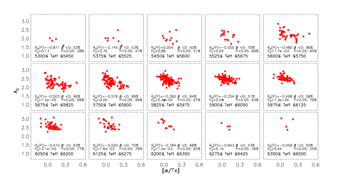
Figure 10: NLTE Li abundance as a function of  [$\alpha$/Fe] in each T_eff bin for our sample stars with Li measurements. The range of T_eff is specified in each plot, with bin size of 150 K. The mean correlation coefficient ($R_{0}(P)$) between A_Li and  [$\alpha$/Fe] , the mean correlation significance level ($P_{0}$), the possibility of Li-$[\alpha/Fe]$ anticorrelation ($\beta$¡0) if consider the abundance uncertainties, and the possibility of P¡0.05 for the anticorrelation are labeled.

It is of great interest to compare the correlation between A_Li and  [$\alpha$/Fe] for stars with similar evolutionary phase (position in the main sequence) as well. We use $\log(g)$ as an index of the evolutionary phase and present the Li- [$\alpha$/Fe] anticorrelation in Fig 11. The $\log(g)$ bin size is 0.235 dex, and is based on a criterion on the $\log(g)$ error that covers 68% of the sample stars. Similar to our treatment for T_eff and [Fe/H] , we overlap half of the bin size between the adjacent bins to avoid selection bias. In each $\log(g)$ interval the mean A_Li - [$\alpha$/Fe] correlation is negative, and the mean correlation significance levels ($P_{0}$) are less than 0.05 except in the first bin which has only a few stars. When taking into account the abundance uncertainties as described above for different T_eff and [Fe/H] bins, there is a (very) high possibility for the Li-$[\alpha/Fe]$ anticorrelation in almost every $\log(g)$ bin.

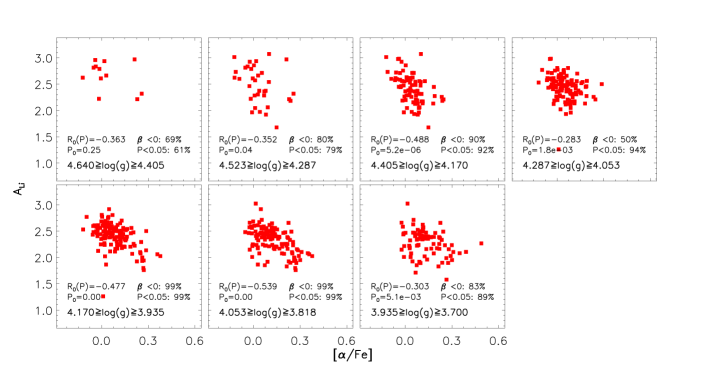
Figure 11: NLTE Li abundance as a function of  [$\alpha$/Fe] in each $\log(g)$ bin for our sample stars with Li measurements. The range of $\log(g)$ is specified in each plot, with bin size of 0.235 dex. The mean correlation coefficient ($R_{0}(P)$) between A_Li and  [$\alpha$/Fe] , the mean correlation significance level ($P_{0}$), the possibility of Li-$[\alpha/Fe]$ anticorrelation ($\beta$¡0) if consider the abundance uncertainties, and the possibility of P¡0.05 for the anticorrelation are labeled.

To ensure that the Li-$[\alpha/Fe]$ anticorrelation echoes the initial A_Li and is not affected by any stellar evolution effect, we check the behaviour of A(Li) in stellar evolution models. We use the latest version of  PARSEC (Bressan et al., 2012; Fu et al., 2017) to calculate Li evolution for two stars with the same metallicity, helium content, stellar mass, initial Li abundance, but one having  [$\alpha$/Fe] =0.4 dex and the other  [$\alpha$/Fe] =0 (solar-scaled). Though the star with  [$\alpha$/Fe] =0.4 dex is hotter in every evolutionary phase (see the left panel of Fig. 12), there is no measurable difference between its A_Li and that of the star with  [$\alpha$/Fe] =0, neither at the same age (see the central panel) nor at the same $\log(g)$ . The different A_Li behaviour in stars with different  [$\alpha$/Fe] has to come from their initial Li abundances which reflect different Li enrichment histories in different disc components.

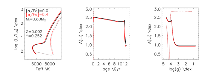
Figure 12: Li evolution from the stellar evolution model  PARSEC . Two stars with the same metallicity and He content (Z=0.002, Y=0.252), the same initial Li abundance (A_Li =2.8 dex), the stellar mass (M_i=0.80 M_⊙), but different $\alpha$-enhancements are compared. The red curves indicate the star with  [$\alpha$/Fe] =0.4 dex while the black ones are for the star with  [$\alpha$/Fe] =0 (solar-scaled). The dotted lines in both colors represent the evolution before the zero-age main sequence (ZAMS), and the solid lines indicate the evolution after. The panels from left to right are HR diagram, A_Li evolution with stellar age, and A_Li as a function of $\log(g)$ , respectively.

The Li-$[\alpha/Fe]$ anticorrelation also sheds light on the role of core collapse SNe in the total Li enrichment. Since core collapse SNe are the main producer of the $\alpha$ elements, if these stars are responsible also for a major Li production, this element should increase with  [$\alpha$/Fe] . Our Li- [$\alpha$/Fe] anticorrelation result, instead, implies that the contribution from core collapse SNe to the global Li enrichment is unimportant, if not negligible, thus supporting previous findings (see the Introduction).

3.3 Li-$s$(-$process\leavevmode\nobreak\ elements$) correlation

Similarly to the  [$\alpha$/Fe] ratio, the ratio of the slow ($s-$) neutron capture process elements to iron can be regarded as a cosmic clock. Ba, Sr , La, and Y are mainly $s-$process elements produced on long timescales by low mass AGB stars (Matteucci, 2012). Since a low mass star must evolve to the AGB phase before the $s-$process can occur, the $s-$process elements are characterized by a delay in the production, much like the delay of iron production by SNe Ia relative to the $\alpha$ elements production by core collapse SNe. Among the four $s-$process elements mentioned above, GES provides the abundances of Y II (the first $s-$process peak element) and Ba II (the second $s-$process peak element) for all our sample stars. Their abundances behave differently in the Galactic thick and thin discs (Bensby et al., 2005; Israelian et al., 2014; Bensby et al., 2014; Bisterzo et al., 2017; Delgado Mena et al., 2017). Unlike the Galactic thick disc stars, which show an almost constant [Ba/Fe] abundance close to the solar value, the Galactic thin disc stars have their [Ba/Fe] abundances increasing with [Fe/H] and reaching their maximum values around solar metallicity, after which a clear decline is seen (see also Cristallo et al., 2015a, b, for the most recent $s-$process calculation in AGB yields). The same trend is observed in our sample. In Fig. 13 we display the Li-[Ba/Fe],  [Ba/Fe] as a function of [Fe/H], and the evolution of absolute Ba abundance A(Ba), as derived from Ba II lines. The same figures are also plotted for yttrium (Y II).  [Ba/Fe] and  [Y/Fe] values here are derived from MCMC simulations, taking into account the measurement uncertainties of A(Ba II)/A(Y II) and [Fe/H] . By applying the same MCMC setups used for  [$\alpha$/Fe] (see Sec.  3.1), we calculate the mean values of  [Ba/Fe] and  [Y/Fe] for each star. These values, together with their corresponding 1 $\sigma$ uncertainties, are listed in Table 2. In the literature there are several theoretical works on the evolution of  [Ba/Fe] and  [Y/Fe] in the Galactic thin disc (e.g. Pagel & Tautvaisiene, 1997; Travaglio et al., 1999, 2004; Cescutti et al., 2006; Maiorca et al., 2012; Bisterzo et al., 2017). For comparison, we show in Fig. 13 the predictions of the most recent one (Bisterzo et al., 2017) who use the updated nuclear reaction network.

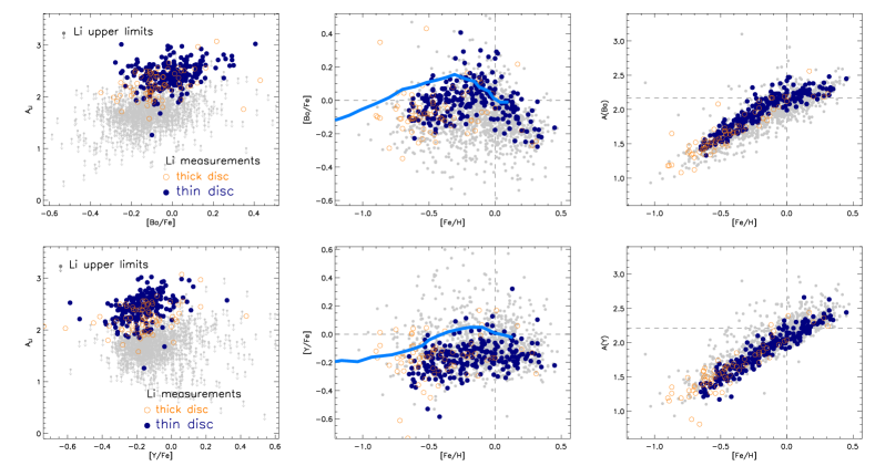
Figure 13: NLTE Li abundance versus  [Ba/Fe] (upper left panel),  [Ba/Fe] against [Fe/H] (upper middle panel), and absolute barium abundance A(Ba) as a function of [Fe/H] (upper right panel). The three lower panels are the same for yttrium. The  [Ba/Fe] and  [Y/Fe] versus [Fe/H] trends predicted by Bisterzo et al. (2017) for the Galactic thin disc are overlaid with light blue solid lines. Dashed lines indicate the solar values. Stars with Li measurements are separated as thick (filled blue dots) and thin (open orange circles) disc stars, as the same as in the middle panel of Fig. 6. The grey dots represent sample stars with Li upper limits.

For stars with true Li measurements (filled blue dots and open orange circles in Fig. 13), their A_Li show a significant overall correlation with  [Ba/Fe] and  [Y/Fe] (at a 99% confidence level). Fig 14 and Fig 15 display the A_Li - [Ba/Fe] and A_Li - [Y/Fe] correlation, respectively, in different [Fe/H] intervals. The anticorrelation is especially significant in the range -0.74$\lesssim$[Fe/H] $\lesssim$0.43 for A_Li - [Ba/Fe] and -0.48$\lesssim$[Fe/H] $\lesssim$0.56 for A_Li - [Y/Fe] . The Li-$s$(-process elements) correlation is easily understood since both of them are produced mostly by long-lived stellar sources (see e.g. Romano et al., 1999, 2001; Bisterzo et al., 2017, and references therein).

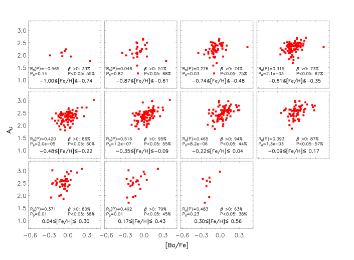
Figure 14: NLTE Li abundance as a function of  [Ba/Fe] in each [Fe/H] bin for our sample stars with Li measurements. The range of [Fe/H] is specified in each plot. The [Fe/H] bin size is 0.26 dex. In each bin the mean correlation coefficient ($R_{0}(P)$) between A_Li and  [Ba/Fe] , the mean correlation significance level ($P_{0}$), the possibility of A_Li - [Ba/Fe] correlation ($\beta$¿0) if consider the abundance uncertainties, and the possibility of P¡0.05 for the anticorrelation are labeled.

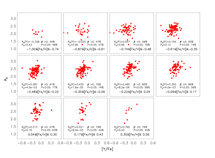
Figure 15: NLTE Li abundance as a function of  [Y/Fe] in each [Fe/H] bin for our sample stars with Li measurements. The range of [Fe/H] is specified in each plot. The [Fe/H] bin size is 0.26 dex. In each bin the mean correlation coefficient ($R_{0}(P)$) between A_Li and  [Y/Fe] , the mean correlation significance level ($P_{0}$), the possibility of A_Li - [Y/Fe] correlation ($\beta$¿0) if consider the abundance uncertainties, and the possibility of P¡0.05 for the anticorrelation are labeled.

The main source for $s$-process elements appear to be low mass AGB stars (Kippenhahn et al., 2012). Given the small [Ba/Fe] enhancement in most of the stars with lower Li which have higher  [$\alpha$/Fe] and probably belong to the thick disc, we conclude that AGB stars may mainly contribute to the chemical enrichment in the Galactic thin disc (with lower  [$\alpha$/Fe] ). Similar results have also been reported by Mashonkina & Gehren (2001); Delgado Mena et al. (2017) and agree with existing theoretical scenarios of relatively fast/slow thick/thin disc formation (see e.g. Micali et al., 2013).

4 Discussion

We show in Sec. 3 that the Galactic thin disc stars have stronger and higher overall level of Li enrichment than the thick disc stars. This result gives us new insights into other observational phenomena, e.g. the ”Li-rich giant problem” (see the introduction) which should be studied separately in different environments for two reasons. First, the definition of ”Li-rich giant” will be affected since the thick and thin disc stars have different initial abundances of Li; second and more important, giant stars in the environment with stronger Li enrichment are more likely to be polluted by external sources (i.e. contamination by the ejecta of nearby novae, Martin et al., 1994). Aguilera-Gómez et al. (2016) calculate red giant models with substellar object engulfment and conclude that a Li enrichment up to A(Li)$\sim$2.2 dex can be explained by engulfing a 15 Jupiter mass ($M_{J}$) substellar object. If we make a simple calculation, a 15 $M_{J}$ substellar object with the initial solar metal mixture contains $M_{Li}\sim$ 2 $\times 10^{-10}$ M_⊙, and a single nova outburst can eject $M_{Li}$=0.3$\sim$4.8 $\times 10^{-10}$M_⊙ (nova V1369 Cen, see Izzo et al., 2015) or $M_{Li}\sim$ 7 $\times 10^{-9}$ M_⊙ (nova V5668 Sgr, see Molaro et al., 2016). A contamination containing 1/30 $\sim$ 7 single nova ejecta provides the same amount of Li as a 15 $M_{J}$ substellar object offers. Furthermore, taking into account that i. the nova ejecta do not increase the stellar angular momentum that introduces mixing and Li burning, and ii. usually a white dwarf can generate multiple novea over time, Li enrichment introduced by novae ejecta contamination is more significant than the substellar objects engulfment. So we expect different frequencies of Li-rich giant stars in different environments.

The upper envelope of the A_Li measurements traced by our sample stars clearly shows that the Galactic Li abundance increases as [Fe/H] approaches the solar value, and then declines for super-solar metallicity objects (see Fig. 5, right panel, and Fig. 7, upper panel). A similar trend is seen also in Ramírez et al. (2012); Delgado Mena et al. (2015); Guiglion et al. (2016). Apparently, these findings contrast with classic Galactic chemical evolution model predictions of a monotonic increase of A_Li with metallicity in the Galactic disc (see Romano et al., 1999, 2001; Travaglio et al., 2001; Prantzos, 2012). Though metal-rich stars have deeper surface convective zone compared to the metal-poor ones with the same stellar mass, it is not likely that the Li decline is due to a stronger Li destruction during the main sequence in the super metal-rich stars because the mean T_eff of these stars are comparable or higher than the solar metallicity ones (see the lower panel of Fig. 7 ). From the stellar physics point of view if the main sequence destruction is not responsible for the Li decline as explained above, the answer may lie in two fields: i. special conditions of mixing and diffusion; and ii. depletion during the pre-main sequence. For the first one, Xiong & Deng (2009) present a non-local convection stellar model that considers a strong overshooting (the bottom boundary is set at a depth deeper than $5\times 10^{6}$ K, which can burn Li efficiently) and pure gravitational settling of microdiffusion, they predict that A(Li) of warm stars (T_eff $>$ 6000K) decreases with increasing T_eff so stars with high T_eff can also have low A(Li). For the second one, Fu et al. (2015) discuss that Li in pre-main sequence stars is first depleted by convection then restored by the residual mass accretion, since the very metal-rich disk has high opacity and is easily evaporated, it is possible that the accretion is terminated early and the Li is not fully restored. In the following, we discuss some possible explanations from the perspective of the Galactic chemical evolution for the observed Li decrease in super-solar metallicity stars, in the framework of the model by Romano et al. (1999, 2001).

In particular, from a close inspection of figures 3 and 4 of Romano et al. (2001), we note that the Li abundance increases with metallicity until [Fe/H] $\sim$ 0, but then decrease for [Fe/H] $>$ 0, in agreement with the trend suggested by our observations. A similar prediction trend is also seen in figure 5 of Abia et al. (1998) with a different choice of yields. The predicted behaviour in Romano et al. (2001, with contributions from both AGB stars and core-collapse SNe) is due to the presence of a threshold in the gas density in their model, below which the star formation stops (see also Chiappini et al., 2001, and reference therein). During the last $\sim 5$ Gyr of evolution, because of the presence of such a threshold, the star formation in the solar neighbourhood has several short periods of activity intercut with star formation gaps. As a consequence, the restitution rate of Li from AGB stars and core-collapse SNe, which tracks rather closely the star formation rate owing to the relatively short lifetimes of the stellar progenitors, is considerably reduced, and the stellar Li astration eventually overcomes the Li production. This star formation gap explanation may hold as well for pure $s$-process elements synthesised in low mass stars, and explains why their abundance relative to iron decreases in super-solar metallicity stars (Fig. 13, the two middle panels; see also Bensby et al., 2005; Bisterzo et al., 2017; Delgado Mena et al., 2017). Furthermore, the absolute abundances of barium show kind of a plateau at super-solar metallicity (see the upper left panel of Fig. 13), which strongly indicates that the production of the $s$-process elements was minor, or even stopped for some time. However, though the NLTE correction has little influence on Ba abundances (Mishenina et al., 2015), stellar activities might affect the A(Ba) trend. Reddy & Lambert (2017) present a strong correlation between the [Ba II/Fe] values and the chromospheric activity for solar-twin stars, they demonstrate that the Ba II abundance of these stars are overestimated because of the adoption of a too low value of microturbulence in the spectrum synthesis. Unfortunately, we are not able to confirm this effect in our sample stars because the stellar activity information is not available. It should also be stressed that the yields of super-solar metallicity stars are not widely investigated in the literature, the yields of $s-$process elements are not very clear. For instance, Cristallo et al. (2015a) present that the yields of the second $s-$process peak (including Ba) mainly contributes to -0.7¡[Fe/H] ¡-0.3 and decreases its contribution at higher metallicities, while Karakas & Lugaro (2016) show that the yields of Ba increase from Z=0.007 to Z=0.03. Further complicating matters, one have to consider also the contribution of low-mass stars that die when the metallicity of the ISM is super-solar, but were born at earlier stages from a metal-poor ISM. Such work requires thorough calculations in the Galactic chemical models.

Still, precise measurements of Li and $s$-process element abundances in stars will be extremely useful to constrain the AGB yields, as well as the Galactic chemical evolution models.

As recently confirmed by the direct detection of Li in the spectra of nova V1369 Cen by Izzo et al. (2015), given the current estimates of the Galactic nova rate, novae might contribute most of the Li in the Galaxy. In particular slow novae, with a rate of around 17 events/yr, would eject in the ISM Li amounts significantly larger than their fast counterparts (Izzo et al., 2015). The nova rate is highly sensitive to the assumed fraction and mass distribution of the binary stellar progenitors. In particular, Gao et al. (2014); Yuan et al. (2015); Gao et al. (2017) report that the fraction of close binaries (which lead to nova outbursts) decreases with increasing [Fe/H]. The super-Chandrasekhar SNe Ia, an end-result of binary stars, also strongly prefer metal-poor environments (Khan et al., 2011). These observations imply that the occurrence of nova systems may be lower at higher metallicities, which would lower the total Li production from such objects in high-metallicity environments. Such a metal-dependence of the nova system formation rate has not been taken into account in Galactic chemical evolution models up to now (Romano et al., 2001; Travaglio et al., 2001). Here we suggest that it could be (co-)responsible for the observed decreasing trend of A_Li for [Fe/H] $>$ 0, a hypothesis that needs to be tested by means of detailed chemical evolution models.

5 Summary

We investigate the Li enrichment histories in the Galactic discs using GES iDR4 data. Li abundance,  [$\alpha$/Fe] ,  [Ba/Fe] , and  [Y/Fe] for 1399 well-measured ([Fe/H] error ¡0.13 dex) main sequence ($\log(g)$ $\leq$ 3.7 dex) field stars with UVES spectra are studied. We divide the sample stars into two categories: Li measurements and Li upper limits. NLTE corrections are applied to the Li line at 6708 Å. Four $\alpha$ elements, Mg, Si, Ca, Ti, are considered in the MCMC calculations to derive the total  [$\alpha$/Fe] and the corresponding 1 $\sigma$ uncertainty. We find a Li- [$\alpha$/Fe] anticorrelation independent of [Fe/H], T_eff , and $\log(g)$ in our sample stars with actual Li measurements. After checking the behaviour of surface Li in stellar evolution models we conclude that different $\alpha$ enhancements do not lead to measurable A_Li differences, thus the Li- [$\alpha$/Fe] anticorrelation echos different levels of Li enrichments in these stars. A Li-$s(-process$ elements) correlation, which is connected to the nucleosynthesis in their common production site (AGB stars), is also seen.

We perform a tentative division based on  [$\alpha$/Fe] and [Fe/H] in order to separate our sample into thick disc stars and thin disc ones. By comparing in each [Fe/H] bin the error-weighted mean A_Li and T_eff values of stars with the highest Li abundance, as well as the fractions of Li-enriched stars, we conclude that the thin disc stars experience a stronger Li enrichment throughout their evolution, compared to the thick disc stars.

The Li decline in super-solar metallicity, which has already been reported by Delgado Mena et al. (2015) and Guiglion et al. (2016), is confirmed by the GES analysis. We discuss the possible explanations of this scenario. It may be a joint consequence of AGB yield evolution and the low binary fraction at a high metallicity.