Improved Density and Distribution Function Estimation

Abstract

Given additional distributional information in the form of moment restrictions, kernel density and distribution function estimators with implied generalised empirical likelihood probabilities as weights achieve a reduction in variance due to the systematic use of this extra information. The particular interest here is the estimation of densities or distributions of (generalised) residuals in semi-parametric models defined by a finite number of moment restrictions. Such estimates are of great practical interest, being potentially of use for diagnostic purposes, including tests of parametric assumptions on an error distribution, goodness-of-fit tests or tests of overidentifying moment restrictions. The paper gives conditions for the consistency and describes the asymptotic mean squared error properties of the kernel density and distribution estimators proposed in the paper. A simulation study evaluates the small sample performance of these estimators. Supplements provide analytic examples to illustrate situations where kernel weighting provides a reduction in variance together with proofs of the results in the paper.

Keywords: Moment conditions, residuals, mean squared error, bandwidth.

MSC 2010 subject classifications: Primary 62G07, secondary 62G05, 62G20.

1 Introduction

In many statistical and economic applications, additional distributional information about the data observation $d_{z}$-vector $z$ may be available in the form of moment restrictions on its distribution. These constraints may arise from a particular economic or physical law, e.g., Chen (1997, Section 5), be implied by estimating equations, Qin and Lawless (1994, Example 1), or correspond to known population moments of another observable random vector correlated with $z$, e.g., in survey samples with auxiliary population information available from census data, e.g., Chen and Qin (1993) and Qin and Lawless (1994, Example 2). The primary purpose of the paper is to explore the advantages of this additional information for the estimation of the density and distribution function of a scalar residual-like function of $z$ which may depend on unknown parameters.

To this end, let $g(z,\beta)$ denote a $d_{g}$-vector of known functions of the data observation $d_{z}$-vector $z\in\mathcal{Z}$ and the $d_{\beta}$-vector $\beta\in\mathcal{B}$ of parameters where the sample space $\mathcal{Z}\subseteq\mathbbm{R}^{d_{z}}$ and parameter space $\mathcal{B}\subset\mathbbm{R}^{d_{\beta}}$ with $d_{\beta}\leq d_{g}$. The moment indicator vector $g(z,\beta)$ will form the basis for inference in the following discussion and analysis. In particular, it is assumed that the true value $\beta_{0}$ taken by $\beta$ uniquely satisfies the population unconditional moment equality condition

$$\operatorname{E}[g(z,\beta_{0})]=0,$$ (1.1)

where $\operatorname{E}[\cdot]$ denotes expectation taken with respect to the true population probability law of $z$. The true parameter value $\beta_{0}$ is generally unknown, but can also be fully or partially known in particular applications.

Models specified in the form of unconditional moment restrictions (1.1) convey partial information about the distribution $F^{z}$ of $z$ and are ubiquitous in economics; see, e.g., the monographs Hall (2005) and Mátyás (1999). Many other commonly used models lead to estimators that can be reformulated as solutions to a set of moment restrictions. Clearly, models given by conditional moment restrictions imply (1.1). Traditionally, such models are estimated by the generalised method of moments (GMM). However, the performance of GMM estimators and associated test statistics is often poor in finite samples, which has lead to the development of a number of (information-theoretic) alternatives to GMM.

This paper focuses on the class of generalised (G) empirical likelihood (EL) estimators, which has attractive large sample properties; see, e.g., Newey and Smith (2004), Smith (1997, 2011), and Parente and Smith (2014) for a recent review. Special cases of GEL include EL, (Owen, 1988, 1990), Qin and Lawless (1994), exponentially tilting (ET), Corcoran (1998), Kitamura and Stutzer (1997), Imbens et al. (1998), and continuous-updating (GMM) estimators (CUE), Hansen et al. (1996); see also Euclidean EL, Antoine et al. (2007). Of these estimators, EL has the attractive property of being Bartlett-correctable; see Chen and Cui (2007).

When the parameter vector $\beta_{0}$ is overidentified by the moment restriction (1.1), i.e., $d_{\beta}<d_{g}$, these constraints generally carry useful additional information about $F^{z}$. Given a random sample $z_{i}$, $i=1,\ldots,n$, of observations on $z$, such information is captured by the associated (G)EL implied probabilities $\pi_{i}$, $i=1,\ldots,n$, which enable a nonparametric description of $F^{z}$ satisfying the moment condition (1.1) given by the estimator $F_{\pi}^{z}(z)=\sum_{i=1}^{n}\pi_{i}\mathbbm{1}\{z_{i}\leq z\}$, where $\mathbbm{1}\{\cdot\}$ denotes the indicator function, Back and Brown (1993), Qin and Lawless (1994). In the absence of the moment information (1.1) or when $\beta_{0}$ is just identified, $d_{\beta}=d_{g}$, $F_{\pi}^{z}(z)$ reduces to the empirical distribution function (EDF) $F_{n}^{z}(z)=n^{-1}\sum_{i=1}^{n}\mathbbm{1}\{z_{i}\leq z\}$. In general, if $d_{\beta}<d_{g}$, $F_{\pi}^{z}(z)$ is a more efficient estimator of $F^{z}$ than the EDF $F_{n}^{z}(z)$ reflecting the value of the overidentifying information in (1.1). This observation suggests therefore that estimation of the functionals of $F^{z}$, $T(F^{z})$, by $T(F_{\pi}^{z})$ rather than $T(F_{n}^{z})$ will be similarly more efficient. Indeed this is the case when estimating expectations of certain known functions of $z$, see Brown and Newey (1998). A similar advantage is apparent for EL estimation of quantile functions with known $\beta_{0}$, e.g., Chen and Qin (1993) and Zhang (1995), general EL-based quantile estimation, Yuan et al. (2014), and EL-based kernel estimation of a univariate density function, e.g., Chen (1997) and Zhang (1998).

The concern of this paper is with efficient kernel estimation of the probability density (p.d.f.) and distribution (c.d.f.) functions of a scalar-valued function $u(z,\beta_{0})$ of the data observation $z$ with either known or unknown parameter vector $\beta_{0}$. The former case, when $\beta_{0}$ is known, is the classical situation briefly mentioned above. The central case of interest, when $\beta_{0}$ is unknown, is estimation of the p.d.f and c.d.f. of an error term based on the estimated residuals. Such estimates are routinely computed by practitioners and are used for both visual diagnostics, e.g., potentially revealing omitted structure such as multimodality or other features of interest, and formal diagnostic tests, e.g., goodness-of-fit and tests of parametric assumptions on the error distribution. The importance of obtaining residual density estimates with good (higher order) properties can hardly be understated. Yet, as discussed below, simply applying standard kernel estimators with default bandwidths to estimated residuals may result in an inconsistent p.d.f. or c.d.f. estimators as further conditions on the kernel function and bandwidth are generally required. Similar conclusions have been reached elsewhere in related literature on residual density estimation in nonparametric regression and other settings; see, e.g., Ahmad (1992), Cheng (2004), Kiwitt et al. (2008), Györfi and Walk (2012) and the discussion and references in Bott et al. (2013).

When $\beta_{0}$ is known, kernel density and distribution function estimators exploiting the (G)EL implied probabilities instead of the uniform EDF $n^{-1}$ weights achieve a reduction of higher order variance due to the systematic use of the extra moment information in (1.1). The efficiency gains are first order asymptotically in the c.d.f. case and second order for p.d.f. estimation. In contradistinction, for residual p.d.f. and c.d.f. estimation, such gains will not always be realised. One can, however, expect efficiency gains from the knowledge that the mean of residuals is zero.

The outline of the paper is as follows. Section 2 briefly describes (G)EL estimation and the associated (G)EL implied probabilities. The main results concerning p.d.f. and c.d.f. estimators are given in Sections 3 and 4 for both known and unknown $\beta_{0}$ cases. The finite sample performance of the proposed estimators is evaluated via a simulation study reported in Section 5. Section 6 concludes. Supplement Supplement LABEL:Supp:Proofs: Proofs and LABEL:Supp:Examples: Examples in the Supplementary Information respectively details some additional assumptions for and the proofs of the results in the main text and analyses a number of examples to illustrate the the properties of the estimators developed in the paper.

2 Generalised Empirical Likelihood

The GEL class of estimators for $\beta_{0}$ is defined in terms of a real valued scalar carrier function $\rho:\mathcal{V}\mapsto\mathbbm{R}$ that is concave on an open interval $\mathcal{V}$ containing zero with derivatives $\rho^{(j)}(v)=\mathrm{d}^{j}\rho(v)/\mathrm{d}v^{j}$ and $\rho_{j}=\rho^{(j)}(0)$, $j=1,2,\ldots$, normalized without loss of generality such that $\rho_{1}=\rho_{2}=-1$. The special cases $\rho(v)=\ln(1-v)$ for $\mathcal{V}=(-\infty,1)$, $\rho(v)=-\exp(v)$ and $\rho(v)=-v^{2}/2-v$ correspond to EL, ET and CUE respectively and are all members of the Cressie and Read (1984) family where $\rho(v)=-(1+\gamma v)^{(\gamma+1)/\gamma}/(\gamma+1)$.

Given a random sample $z_{i}$, $i=1,\ldots,n$, of size $n$ of observations on the $d_{z}$-dimensional vector $z$, let $g_{i}(\beta)=g(z_{i},\beta)$, $g_{i}=g_{i}(\beta_{0})$, and $G_{i}(\beta)=\partial g(z_{i},\beta)/\partial\beta^{\top}$, $G_{i}=G_{i}(\beta_{0})$, $i=1,\ldots,n$. Also let $\Lambda_{n}(\beta)=\{\lambda:\lambda^{\top}g_{i}(\beta)\in\mathcal{V},i=1,\ldots,n\}$. The GEL criterion $P_{n}(\beta,\lambda)$ is defined by $P_{n}(\beta,\lambda)=n^{-1}\sum_{i=1}^{n}\rho(\lambda^{\top}g_{i}(\beta))-\rho(0)$, with $\lambda$ a $d_{g}$-vector of auxiliary parameters, each element of which corresponding to an element of the moment function vector $g(z,\beta)$; for members of the Cressie and Read (1984) family of power divergence criteria $\lambda$ is the Lagrange multiplier vector associated with imposition of the moment restriction (1.1). The GEL estimator $\hat{\beta}$ is the solution to the saddle point problem

$$\hat{\beta}=\operatorname*{argmin}_{\beta\in\mathcal{B}}\sup_{\lambda\in\Lambda_{n}(\beta)}P_{n}(\beta,\lambda).$$ (2.1)

If Supplement LABEL:Supp:Proofs: Assumptions A.1 and A.2 are satisfied, in particular, the population Jacobian $G=\operatorname{E}[\partial g(z,\beta_{0})/\partial\beta^{\top}]$ and variance $\Omega=\operatorname{E}[g(z,\beta_{0})g(z,\beta_{0})^{\top}]$ matrices are full column rank and positive definite respectively, then all GEL estimators share the same first order large sample properties, see, e.g., Newey and Smith (2004, Theorems 3.1 and 3.2), i.e., $n^{1/2}(\hat{\beta}-\beta_{0})\xrightarrow{d}N(0,\Sigma)$, achieving the semiparametric efficiency lower bound $\Sigma=(G^{\top}\Omega^{-1}G)^{-1}$, Chamberlain (1987, Theorem 2). Furthermore, if the additional Supplement LABEL:Supp:Proofs: Assumption A.3 is imposed, defining $H=\Sigma G^{\top}\Omega^{-1}$ and $P=\Omega^{-1}-\Omega^{-1}G(G^{\top}\Omega^{-1}G)^{-1}G^{\top}\Omega^{-1}$, the second order bias of $\hat{\beta}$ is $\operatorname{E}[\hat{\beta}]-\beta_{0}=n^{-1}H\zeta_{\lambda}+\mathit{O}(n^{-2})$, where

$$\zeta_{\lambda}=-a+\operatorname{E}[G_{i}Hg_{i}]+c_{\rho}\operatorname{E}[g_{i}g_{i}^{\top}Pg_{i}],$$ (2.2)

with $c_{\rho}=1+\rho_{3}/2$ and $a$ a $d_{g}$-vector with elements $a^{j}=\mathop{\mathrm{tr}}(\Sigma\operatorname{E}[\partial^{2}g^{j}(z,\beta_{0})/\partial\beta\partial\beta^{\top}])$, $j=1,\ldots,d_{g}$; see Newey and Smith (2004, Theorem 4.2).

Remark 2.1.

The validity of the higher order bias and variance calculations, and hence the validity of the results reported below can be formally justified by that of an Edgeworth expansion of order $\mathit{o}(n^{-1})$ for the distribution of GEL parameter estimators. If $z$ is continuously distributed, appropriate conditions may be found in Bhattacharya and Ghosh (1978) for general smooth functions of sample moments and Kundhi and Rilstone (2012) for Edgeworth expansions for (G)EL estimators. If some of the elements of $z$ are discretely distributed, Jensen (1989) provides appropriate conditions.

For given $\beta$, the auxiliary parameter estimator is defined by $\lambda(\beta)=\operatorname*{argmax}_{\lambda\in\Lambda_{n}(\beta)}P_{n}(\beta,\lambda)$. Whenever the constraint in $\lambda\in\Lambda_{n}(\beta)$ is not binding, $\lambda(\beta)$ solves the first-order conditions
$n^{-1}\sum_{i=1}^{n}\rho^{(1)}(\lambda(\beta)^{\top}g_{i}(\beta))g_{i}(\beta)=0$. The GEL implied probabilities are then

$$\pi_{i}(\beta)=\frac{\rho^{(1)}(\lambda(\beta)^{\top}g_{i}(\beta))}{n^{-1}{\textstyle\sum}_{j=1}^{n}\rho^{(1)}(\lambda(\beta)^{\top}g_{j}(\beta))},\quad i=1,\ldots,n.$$

The sample moment constraint $\sum_{i=1}^{n}\pi_{i}(\beta)g_{i}(\beta)=0$ holds whenever the first order conditions for $\lambda(\beta)$ hold. In what follows, $\hat{\pi}_{i}=\pi_{i}(\hat{\beta})$, $i=1,\ldots,n$, corresponds to the solution $\hat{\lambda}=\lambda(\hat{\beta})$, and, if $\beta_{0}$ is known, $\tilde{\pi}_{i}=\pi_{i}(\beta_{0})$, $i=1,\ldots,n$, with auxiliary parameter estimator $\tilde{\lambda}=\lambda(\beta_{0})$. The generic notation $\pi_{i}$, $i=1,\ldots,n$, is used whenever the distinction is unnecessary.

Remark 2.2.

Properties of the GEL implied probabilities relevant to the subsequent developments are summarized in Supplement LABEL:Supp:Proofs: Lemmas A.1 and A.2. Although $\pi_{i}(\beta)$, $i=1,\ldots,n$, sum to unity and are positive if $\pi_{i}(\beta)g_{i}(\beta)$ is small uniformly in $i$, they are not guaranteed to be non-negative. The shrinkage estimator $\pi_{i}^{\varepsilon}=(\pi_{i}+\varepsilon_{n})/\sum_{j=1}^{n}(\pi_{j}+\varepsilon_{n})$, $i=1,\ldots,n$, where $\varepsilon_{n}=-\min[\min_{1\leq i\leq n}\pi_{i},0]$, see Antoine et al. (2007), Smith (2011), ensures non-negativity $\pi_{i}^{\varepsilon}\geq 0$, $i=1,\ldots,n$, and $\sum_{i=1}^{n}\pi_{i}^{\varepsilon}=1$. Alternative solutions relevant to probability density and distribution function estimation respectively are discussed in Sections 3 and 4.

Remark 2.3.

The implied probabilities were given for EL by Owen (1988), for ET by Kitamura and Stutzer (1997), for quadratic $\rho(\cdot)$ by Back and Brown (1993), and for the general case in the 1992 working paper version of Brown and Newey (2002); see also Smith (1997). For any function $a(z,\beta)$ and GEL estimator $\hat{\beta}$ the implied probabilities can be used to form a semiparametrically efficient estimator $\sum_{i=1}^{n}\hat{\pi}_{i}a(z_{i},\hat{\beta})$ of $\operatorname{E}[a(z,\beta_{0})]$ as in Brown and Newey (1998).

3 GEL-Based Density Estimation

Suppose the p.d.f. $f(\cdot)$ of the scalar random variable $u=u(z,\beta_{0})$ is of interest, where the scalar function $u:\mathcal{Z}\times\mathcal{B}\mapsto\mathcal{U}\subseteq\mathbbm{R}$ is known up to the parameter vector $\beta_{0}$.

Let $\mathcal{N}$ denote an open neighbourhood of $\beta_{0}$.

Assumption 3.1.

For all $\beta\in\mathcal{N}$ there exists a function $v:\mathcal{Z}\times\mathcal{B}\mapsto\mathcal{V}\subseteq\mathbbm{R}^{d_{z}-1}$ such that the vector of functions $(u(z,\beta),\>v(z,\beta)^{\top})^{\top}$ is a bijection between $\mathcal{Z}$ and $\mathcal{U}\times\mathcal{V}$.

Remark 3.1.

Equivalently Assumption 3.1 may be restated as requiring that for every $\beta\in\mathcal{N}$ there exists a bijection between $z$ and some $d_{z}$-vector $w=w(z,\beta)$ such that, given $\{w^{j}(z,\beta)\}_{j=2}^{d_{z}}$, $u(z,\beta)$ and $w^{1}(z,\beta)$ are bijective. That is to say, $z$ may be solved for uniquely given values for $u$, $v$ and $\beta$.

Remark 3.2.

A function $u(z,\beta)$ satisfying Assumption 3.1 may be thought of as defining a generalised residual in the sense of Cox and Snell (1968) and Loynes (1969), with $\hat{u}_{i}=u(z_{i},\hat{\beta})$, $i=1,\ldots,n$, the estimated residuals. Of course, other possibilities of interest are included, e.g., estimating the density of an element of $z$ subject to the extra information available in the moment condition (1.1).

3.1 Known $\beta_{0}$

Suppose that $u_{i}=u(z_{i},\beta_{0})$, $i=1,\ldots,n$, are observed. Then the classical kernel density estimator for the p.d.f. $f$ of $u=u(z,\beta_{0})$ can be employed; viz.

$$\tilde{f}(u)=n^{-1}{\textstyle\sum}_{i=1}^{n}k_{b}(u-u_{i}),$$ (3.1)

where $k_{b}(x)=k(x/b)/b$, $k(\cdot)$ is a kernel function and $b=b_{n}>0$ is a bandwidth sequence; see Rosenblatt (1956) and Parzen (1962). The estimator $\tilde{f}$ (3.1) will serve as a benchmark for later comparisons.

The properties of $\tilde{f}$ are well known and can be formally established under different combinations of smoothness and integrability conditions on the kernel $k$ and density $f$; see, e.g., Rao (1983, Section 2.1). A standard set of such conditions is given in Assumption 3.2 below. If $k$ is square integrable, but not absolutely integrable, as is the case for the sinc kernel, conditions such as those in Tsybakov (2009, Theorem 1.5) can be imposed.

Let $R(k)=\int_{-\infty}^{\infty}k(x)^{2}\mathrm{d}x$ for any square integrable function $k$; the limits of integration are omitted whenever there is little scope for confusion. Also let $f^{(j)}(u)=\mathrm{d}^{j}f(u)/\mathrm{d}u^{j}$ for any $j$th order differentiable function $f$.

Assumption 3.2.

(a)(i) $\sup_{-\infty<x<\infty}\lvert k(x)\rvert<\infty$, $\int\lvert k(x)\rvert\mathrm{d}x<\infty$, $\int k(x)\mathrm{d}x=1$, and $\lim_{\lvert x\rvert\to\infty}\lvert xk(x)\rvert=0$; (ii) $k$ is a $(2r)$th order kernel, i.e., an even function such that, for some $r\geq 1$, $\mu_{0}(k)=1$, $\mu_{j}(k)=0$, $j=1,\ldots,2r-1$, and $\mu_{2r}(k)<\infty$, where $\mu_{j}(k)=\int x^{j}k(x)\mathrm{d}x$; (iii) $R(k)<\infty$; (b) $f(\cdot)$ is $s$ times continuously differentiable and $R(f^{(j)})<\infty$, $j=0,1,\ldots,s$. (c) as $n\to\infty$, $b\to 0$ and $nb\to\infty$.

Remark 3.3.

If Assumption 3.2(a)(i) holds, then by Supplement LABEL:Supp:Proofs: Lemma A.3, $\operatorname{E}[\tilde{f}(u)]\to f(u)$ as $b\to 0$ at all points $u$ of continuity of $f$ and if, in addition, Assumption 3.2(c) holds, then the mean squared error (MSE), $\operatorname{MSE}[\tilde{f}(u)]=\operatorname{E}[(\tilde{f}(u)-f(u))^{2}]\to 0$ as $n\to\infty$; see, e.g., Parzen (1962).

Remark 3.4.

Higher order approximations to $\operatorname{MSE}[\tilde{f}(u)]$ can be obtained if $f$ is sufficiently smooth. See, e.g. Rao (1983, Theorem 2.1.5), Wand and Jones (1995, Section 2.8) or Pagan and Ullah (1999, Section 2.4.3). The idea of using higher order kernels as a bias reduction technique originates at least as far back as Bartlett (1963).

Let $1\leq r<\infty$. Suppose that Assumptions 3.2(a)(ii), 3.2(b) with $s=2r+2$, 3.2(c) together with $\mu_{2r+2}(k)<\infty$ and $\int x^{2}k(x)^{2}\mathrm{d}x<\infty$ hold. Then

$$\operatorname{E}[\tilde{f}(u)] =f(u)+(2r)!^{-1}\mu_{2r}(k)f^{(2r)}(u)b^{2r}+\mathit{O}(b^{2r+2}),$$

$$\operatorname{Var}[\tilde{f}(u)] =(nb)^{-1}R(k)f(u)-n^{-1}f(u)^{2}+\mathit{O}(n^{-1}b).$$

Hence,

$$\operatorname{MSE}[\tilde{f}(u)]=(nb)^{-1}R(k)f(u)+(2r)!^{-2}\mu_{2r}(k)^{2}f^{(2r)}(u)^{2}b^{4r}-n^{-1}f(u)^{2}+\mathit{O}(b^{4r+2}\vee n^{-1}b).$$ (3.2)

Remark 3.5.

If $k$ is a $(2r)$th order kernel and Assumption 3.2(b) holds with $s=2r$, the remainder term in $\operatorname{E}[\hat{f}(u)]$ is $\mathit{o}(b^{2r})$. The $\sim n^{-1}$ term is kept explicit with $\mathit{O}$ remainder for reasons that will become apparent below.

The mean integrated squared error (MISE), $\operatorname{MISE}[\tilde{f}]=\operatorname{E}[\int(\tilde{f}(u)-f(u))^{2}\mathrm{d}u]$, is a commonly used global measure of performance. The optimal bandwidth is then defined as that value of $b>0$ minimising MISE, or an approximation thereof. In particular, the asymptotically optimal bandwidth is defined as the value $b^{\ast}$ minimising the two leading terms in the expansion

$$\operatorname{MISE}[\tilde{f}(\cdot;b)]=(nb)^{-1}R(k)+(2r)!^{-2}\mu_{2r}(k)^{2}R(f^{(2r)})b^{4r}-n^{-1}R(f)+\mathit{O}(b^{4r+2}\vee n^{-1}b),$$ (3.3)

i.e., $b^{\ast}=cn^{-1/(4r+1)}$ where $c=[(2r)!^{2}R(k)/(4r\mu_{2r}(k)^{2}R(f^{(2r)})]^{1/(4r+1)}$. The asymptotically optimal MISE is thereby

$$\operatorname{MISE}[\tilde{f}(\cdot;b^{\ast})]=n^{-4r/(4r+1)}c^{-1}R(k)\left[1+(4r)^{-1}\right]-n^{-1}R(f)+\mathit{O}(n^{-1-1/(4r+1)}).$$

Remark 3.6.

If $k$ is of order greater than two, it necessarily takes negative values. Hence $\tilde{f}$ (3.1) itself need not be a density function. Note, however, that the positive part estimator, $\tilde{f}^{+}(u)=\max[\tilde{f}(u),0]$ has MSE at most equal to $\operatorname{MSE}[\tilde{f}(u)]$. Further modifications that ensure integration to unity can be applied as described in Glad et al. (2003).

The GEL-based kernel density estimator incorporates the information embedded in the moment restriction (1.1) replacing the sample EDF weights $n^{-1}$ in the construction of $\tilde{f}(u)$ (3.1) by the implied probabilities $\tilde{\pi}_{i}$, $i=1,\ldots,n$; viz.

$$\tilde{f}_{\rho}(u)={\textstyle\sum}_{i=1}^{n}\tilde{\pi}_{i}k_{b}(u-u_{i})$$ (3.4)

Remark 3.7.

The GEL-based kernel density estimator $\tilde{f}_{\rho}(u)$ (3.4) is the estimator of $f(u)$ obtained from the revised GEL criterion $\sum_{i=1}^{n}[\rho(\eta(f(u)-k_{b}(u-u_{i}))+\lambda^{\top}g_{i}(\beta))-\rho(0)]/n$ with the implicit moment condition $\operatorname{E}[k_{b}(u-u_{i})]=f(u)$ and associated auxiliary parameter $\eta$; see Smith (2011, Section 3).

Remark 3.8.

If the validity of the moment restriction (1.1) is in doubt, a pre-test can be conducted using the GEL-based criterion (2.1) paralleling the classical likelihood ratio test; see, e.g., Kitamura and Stutzer (1997), Imbens et al. (1998) and Smith (1997, 2011). For example, under the null hypothesis that (1.1) holds for some unique $\beta_{0}\in\mathcal{B}$, the normalised GEL criterion (2.1) evaluated at the estimated parameters, $2nP_{n}(\hat{\beta},\hat{\lambda})$, is asymptotically chi-square distributed with $d_{g}-d_{\beta}$ degrees of freedom. The parametric null hypothesis of known $\beta_{0}=\beta^{0}$ can be tested at the $\alpha$ level using the critical region $\{2nP_{n}(\beta^{0},\tilde{\lambda})\geq\chi_{d_{\beta}}^{2}(\alpha)\}$.

To describe the properties of GEL-based kernel density estimator $\tilde{f}_{\rho}(u)$ (3.4), the shorthand notation, e.g., $\operatorname{E}[g_{i}|u]=\operatorname{E}[g(z,\beta_{0})|\{z:u(z,\beta_{0})=u\}]$, for conditional expectations given $u$ is adopted.

Theorem 3.1.

If Supplement LABEL:Supp:Proofs: Assumptions A.1–A.3 and 3.2(a)(i) and (c) are satisfied, then $\tilde{f}_{\rho}(u)=\tilde{f}(u)+\mathit{o}_{p}(1)$ for all $u$ such that $f(u)<\infty$. If, in addition, Assumption 3.1 is satisfied, then

$$\mkern-10.0mu\operatorname{E}[\tilde{f}_{\rho}(u)] =\operatorname{E}[\tilde{f}(u)]+n^{-1}c_{\rho}\left(-\operatorname{E}[g_{i}^{\top}\Omega^{-1}g_{i}|u]+\operatorname{E}[g_{i}^{\top}\Omega^{-1}g_{i}g_{i}^{\top}]\Omega^{-1}\operatorname{E}[g_{i}|u]+d_{g}\right)f(u)+\mathit{o}(n^{-1}),$$ (3.5)

$$\mkern-10.0mu\operatorname{Var}[\tilde{f}_{\rho}(u)] =\operatorname{Var}[\tilde{f}(u)]-n^{-1}\operatorname{E}[g_{i}|u]^{\top}\Omega^{-1}\operatorname{E}[g_{i}|u]f(u)^{2}+\mathit{o}(n^{-1}).$$ (3.6)

Thus, the estimators $\tilde{f}$ and $\tilde{f}_{\rho}$ are asymptotically first-order equivalent, and the asymptotically optimal bandwidth for $\tilde{f}_{\rho}$ is identical to that of $\tilde{f}$, i.e., $b^{\ast}$.

Whenever $c_{\rho}=0$, as is the case for (G)EL with $\rho_{3}=-2$ , e.g., EL, the $n^{-1}$ bias term in (3.5) vanishes. In general, provided the bandwidth does not go to zero faster than $n^{-1/(2r)}$, and certainly when $b=b^{\ast}\sim n^{-1/(4r+1)}$, this bias term is at most third order. Its contribution to MISE is via the integrated squared bias (ISB)

$$\operatorname{ISB}[\tilde{f}_{\rho}] =\operatorname{ISB}[\tilde{f}]+n^{-1}b^{2r}c_{\rho}2(2r)!^{-1}\mu_{2r}(k)\int\left(-\operatorname{E}[g_{i}^{\top}\Omega^{-1}g_{i}|u]\right.$$

$$\quad\left.+\operatorname{E}[g_{i}^{\top}\Omega^{-1}g_{i}g_{i}^{\top}]\Omega^{-1}\operatorname{E}[g_{i}|u]+d_{g}\right)f^{(2r)}(u)f(u)\mathrm{d}u+\mathit{o}(n^{-1}b^{2r}\vee n^{-2}),$$

with the $\mathit{O}(n^{-1}b^{2r})$ term generally non-zero and either positive or negative. With the asymptotically optimal bandwidth, $n^{-1}(b^{\ast})^{2r}\sim n^{-3/2+1/(8r+2)}$, which approaches $n^{-3/2}$ arbitrarily closely as $r$ increases, whereas the leading terms in $\operatorname{MISE}[\tilde{f}(\cdot;b^{\ast})]$ becomes arbitrarily close to $n^{-1}$.

As long as $\operatorname{E}[g_{i}|u]\neq 0$, the GEL-based estimator $\tilde{f}_{\rho}$ enjoys a second-order reduction in variance due to the $n^{-1}$ term in (3.6), which does not depend on the choice of GEL carrier function $\rho(\cdot)$. Hence

$$\operatorname{MISE}[\tilde{f}_{\rho}]=\operatorname{MISE}[\tilde{f}]-n^{-1}{\textstyle\int}\operatorname{E}[g_{i}|u]^{\top}\Omega^{-1}\operatorname{E}[g_{i}|u]f(u)^{2}\mathrm{d}u+\mathit{o}(n^{-1}).$$

While this reduction is negligible asymptotically, the leading term in $\operatorname{MISE}[\tilde{f}]$ approaches zero only a little more slowly than $n^{-1}$. Hence the effect could be substantial in small samples.

3.2 Unknown $\beta_{0}$

Suppose now that $\beta_{0}$ is unknown. Then, after substitution of the estimators $\hat{u}_{i}=u(z_{i},\hat{\beta})$ for $u_{i}$, $i=1,\ldots,n$, in $\tilde{f}$ and $\tilde{f}_{\rho}$ in (3.1) and (3.4), the analogous estimators of $f(u)$ are

$$\hat{f}(u) =n^{-1}{\textstyle\sum}_{i=1}^{n}k_{b}(u-\hat{u}_{i}),$$ (3.7)

$$\hat{f}_{\rho}(u) ={\textstyle\sum}_{i=1}^{n}\hat{\pi}_{i}k_{b}(u-\hat{u}_{i}),$$ (3.8)

respectively. Because $u_{i}$, $i=1,\ldots,n$, are not directly observable, the behaviour of the estimation error $\hat{u}_{i}-u_{i}$, $i=1,\ldots,n$, needs to be constrained with additional restrictions imposed on $k$ and $b$. Assumption 3.3 gives a set of mild sufficient conditions, see, e.g., Van Ryzin (1969) and Ahmad (1992); similar conditions have also been considered in, e.g., Cheng (2005) and Kiwitt et al. (2008).

Assumption 3.3.

(a) $k$ is Hölder continuous with exponent $0<\tau\leq 1$; (b) there exists $d(z)\geq 0$ with $\operatorname{E}[d(z)^{\tau}]<\infty$ such that, for some $0<\alpha\leq 1$, $\lvert u(z,\beta)-u(z,\beta_{0})\rvert\leq d(z)\lVert\beta-\beta_{0}\rVert^{\alpha}$ for all $z$ and for all $\beta\in\mathcal{N}$; (c) $b\to 0$ and $n^{\alpha\tau/2}b^{1+\tau}\to\infty$ as $n\to\infty$.

The uniform $\alpha$-Hölder condition Assumption 3.3(b) on $u(z,\beta)$, also known as a Lipschitz condition of order $\alpha$, is an appropriate way to quantify the ‘degree of continuity’ of $u(z,\beta)$; see Zygmund (2003, pp.42–45). Many kernels used in practice are Lipschitz continuous, and hence satisfy Assumption 3.3(a) with $\tau=1$. For example, a kernel that satisfies Assumption 3.3(a) for any $0<\tau\leq\gamma$ but not for $\gamma<\tau\leq 1$ is $k(x)=(1+\gamma)(1-\lvert x\rvert)^{\gamma}/2$ if $\lvert x\rvert\leq 1$ and $0$ otherwise, yielding the Bartlett (triangular) kernel if $\gamma=1$. Assumption 3.3(c) is important as it prevents the bandwidth from being too small. Intuitively, if $b$ is very small, the kernel $k_{b}(u-\hat{u}_{i})$ is very narrowly centered around the incorrect value $\hat{u}_{i}$ potentially excluding the true value $u_{i}$; see, e.g., Silverman (1986, Figure 2.5) for a generic illustration. Assumption 3.3(c) requires $nb^{4}\to\infty$ regardless of the values of $\tau$ and $\alpha$ and $b=n^{-1/4}$ is the fastest rate achievable when $\alpha=\tau=1$. Note that the optimal bandwidth $b^{\ast}$ is excluded if $[\alpha(4r+1)-2]\tau<2$.

Under these conditions, Theorem 3.2 establishes that the differences between the kernel density estimators $\hat{f}$ (3.7) and $\hat{f}_{\rho}$ (3.8) and their counterparts $\tilde{f}$ (3.1) and $\tilde{f}_{\rho}$ (3.4) based on observable $u_{i}$, $i=1,\ldots,n$, are negligible asymptotically.

Theorem 3.2.

If Supplement LABEL:Supp:Proofs: Assumptions A.1–A.3 and 3.3 are satisfied, then $\hat{f}(u)=\tilde{f}(u)+\mathit{o}_{p}(1)$ and $\hat{f}_{\rho}(u)=\sum_{i=1}^{n}\hat{\pi}_{i}k_{b}(u-u_{i})+\mathit{o}_{p}(1)$ for all $u$. If, in addition, Assumption 3.2(a)(i) holds, $\hat{f}_{\rho}(u)=\tilde{f}(u)+\mathit{o}_{p}(1)$ a.e.

To obtain higher order expansions for the mean and variance of $\hat{f}(u)$ (3.7) and $\hat{f}_{\rho}(u)$ (3.8) requires a further strengthening of the assumptions. Let $\nabla u(z,\beta)$ and $\nabla^{2}u(z,\beta)$ denote respectively the $d_{\beta}$-vector and $d_{\beta}\times d_{\beta}$ matrix of the first and second derivatives of $u(z,\beta)$ with respect to $\beta$. Also let $\nabla u_{i}=\nabla u(z_{i},\beta_{0})$ and $\nabla^{2}u_{i}=\nabla^{2}u(z_{i},\beta_{0})$.

Assumption 3.4.

(a) $k$ is twice differentiable and $k^{(2)}$ is Hölder continuous with exponent $0<\tau\leq 1$, $k$, $k^{(1)}$, and $k^{(2)}$ are absolutely integrable; $\lim_{\lvert x\rvert\to\infty}\lvert x^{s}k^{(s-1)}(x)\rvert=0$, $s=1,2,3$, and $\int k(x)\mathrm{d}x=1$; (b) $u(z,\beta)$ is twice differentiable for all $\beta\in\mathcal{N}$, $\operatorname{E}[\lVert\nabla u_{i}\rVert^{4}]<\infty$, $\operatorname{E}[\lVert\nabla^{2}u_{i}\rVert^{4}]<\infty$, and there exists $d(z)\geq 0$ with $\operatorname{E}[d(z)^{4}]<\infty$ such that, for some $0<\alpha\leq 1$, $\lVert\nabla^{2}u(z,\beta)-\nabla^{2}u(z,\beta_{0})\rVert\leq d(z)\lVert\beta-\beta_{0}\rVert^{\alpha}$ for all $z$ and for all $\beta\in\mathcal{N}$; (c) $b\to 0$ as $n\to\infty$, $n^{\tau/2}b^{3+\tau}\to\infty$, and $n^{\alpha/2}b^{5/4}\to\infty$; (d)(i) $f$ is twice differentiable; (ii) $\operatorname{E}[\nabla u_{i}|u]$, $\operatorname{E}[\nabla^{\top}u_{i}Hg_{i}|u]$, and $\operatorname{E}[\nabla^{2}u_{i}|u]$ are differentiable in $u$ and $\operatorname{E}[\nabla u_{i}\nabla^{\top}u_{i}|u]$ is twice differentiable in $u$; (iii) $\mathrm{d}\{\operatorname{E}[\nabla u_{i}|u]f(u)\}/\mathrm{d}u$, $\mathrm{d}\{\operatorname{E}[\nabla^{\top}u_{i}Hg_{i}|u]f(u)\}/\mathrm{d}u$, $\mathrm{d}\{\operatorname{E}[\nabla^{2}u_{i}|u]f(u)\}/\mathrm{d}u$, and $\mathrm{d}^{2}\{\operatorname{E}[\nabla u_{i}\nabla^{\top}u_{i}|u]f(u)\}/\mathrm{d}u^{2}$ are absolutely integrable functions of $u$.

Assumption 3.4(a)(b) implies Assumption 3.3(a)(b) holds with $\alpha=\tau=1$ with the requirement in Assumption 3.3(c) rendered as $n^{1/2}b^{2}\to\infty$. Note that Assumption 3.4(a) also implies Assumption 3.2(a)(i). Assumption 3.4(d) imposes additional smoothness and integrability conditions on $f$ and $u(z,\beta)$. Assumption 3.4(c) is much stronger than Assumption 3.3(c) requiring $nb^{8}\to\infty$ regardless of the values of $\tau$ and $\alpha$ thereby prohibiting the asymptotically optimal bandwidth $b^{\ast}$ when $k$ is a second order kernel. For $r\geq 2$, $b^{\ast}$ is permissible as long as $\tau>6/(4r-1)$ and $\alpha>5/(8r+2)$. Note that, if $\alpha>5/16$, $n^{\tau/2}b^{3+\tau}\to\infty$ implies $n^{\alpha/2}b^{5/4}\to\infty$.

Theorem 3.3.

If Supplement LABEL:Supp:Proofs: Assumptions A.1–A.3, 3.1, and 3.4 are satisfied, then $\operatorname{E}[\hat{f}(u)]=\operatorname{E}[\tilde{f}(u)]+n^{-1}\delta(u)+\mathit{o}(n^{-1})$ and $\operatorname{E}[\hat{f}_{\rho}(u)]=\operatorname{E}[\tilde{f}(u)]+n^{-1}\delta(u)+n^{-1}\delta_{\rho}(u)+\mathit{o}(n^{-1})$, where

$$\delta(u) =\mathrm{d}\{\operatorname{E}[\nabla^{\top}u_{i}Hg_{i}|u]f(u)\}/\mathrm{d}u-\zeta_{\lambda}^{\top}H^{\top}[\mathrm{d}\{\operatorname{E}[\nabla u_{i}|u]f(u)\}/\mathrm{d}u]$$

$$\quad+\tfrac{1}{2}\mathop{\mathrm{tr}}(\Sigma[\mathrm{d}^{2}\{\operatorname{E}[\nabla u_{i}\nabla^{\top}u_{i}|u]f(u)\}/\mathrm{d}u^{2}-\mathrm{d}\{\operatorname{E}[\nabla^{2}u_{i}|u]f(u)\}/\mathrm{d}u])$$ (3.9)

and

$$\delta_{\rho}(u) =(-c_{\rho}\operatorname{E}[g_{i}^{\top}Pg_{i}|u]+c_{\rho}(d_{g}-d_{\beta})+\zeta_{\lambda}^{\top}P\operatorname{E}[g_{i}|u])f(u).$$ (3.10)

Also

$$\operatorname{Var}[\hat{f}(u)] =\operatorname{Var}[\tilde{f}(u)]+n^{-1}[\mathrm{d}\{\operatorname{E}[\nabla u_{i}|u]f(u)\}/\mathrm{d}u]^{\top}\Sigma[\mathrm{d}\{\operatorname{E}[\nabla u_{i}|u]f(u)\}/\mathrm{d}u]$$

$$\quad+n^{-1}2[\mathrm{d}\{\operatorname{E}[\nabla u_{i}|u]f(u)\}/\mathrm{d}u]^{\top}H\operatorname{E}[g_{i}|u]f(u)+\mathit{o}(n^{-1}),$$ (3.11)

$$\operatorname{Var}[\hat{f}_{\rho}(u)] =\operatorname{Var}[\hat{f}(u)]-n^{-1}\operatorname{E}[g_{i}|u]^{\top}P\operatorname{E}[g_{i}|u]f(u)^{2}+\mathit{o}(n^{-1}).$$ (3.12)

Remark 3.9.

The general conclusion of Theorem 3.3 for both bias and variance is identical to that of Theorem 3.1, i.e., the estimation effects of substituting $\hat{u}_{i}$ for $u_{i}$, $i=1,\ldots,n$, and the GEL implied probabilities $\hat{\pi}_{i}$ for $\tilde{\pi}_{i}$, $i=1,\ldots,n$, are both of order $n^{-1}$. The bias term in $\hat{f}$ induced by estimation is similar to that for $\tilde{f}$ in Theorem 3.1 except that $P$ in (3.10) replaces $\Omega^{-1}$ in (3.5) and two extra terms enter via $\zeta_{\lambda}$, viz. $-a$ and $\operatorname{E}[G_{i}Hg_{i}]$ in (2.2). These latter terms appear in the higher order asymptotic bias $n^{-1}H(-a+\operatorname{E}[G_{i}Hg_{i}])$ for the infeasible GEL estimator based on the optimal moment indicator vector $G^{\top}\Omega^{-1}g(z,\beta)$, see Newey and Smith (2004, Theorem 4.2), and are inherited by all GEL estimators. Unlike Theorem 3.1 for the known $\beta_{0}$ case, this term no longer vanishes for a particular choice of a carrier function $\rho$. The replacement of $\Omega^{-1}$ by $P$ represents the loss of information occasioned by the estimation of $\beta_{0}$. In a number of cases, the term $\operatorname{E}[g_{i}|u]^{\top}P\operatorname{E}[g_{i}|u]$ may vanish, see, e.g., Supplement LABEL:Supp:Examples: Example B.3. This of course always occurs for an exactly identified model $d_{g}=d_{\beta}$ since $\hat{\pi}_{i}=n^{-1}$ and $\hat{f}_{\rho}$ (3.8) and $\hat{f}$ (3.7) are identical. However, see Supplement LABEL:Supp:Examples: Example B.4, in general $\hat{f}_{\rho}$ may still enjoy a second-order reduction in variance due to the systematic use of overidentifying moment information (1.1).

The extra bias term $\delta(u)$ (3.9) for $\hat{f}_{\rho}$ and those terms appearing in $\operatorname{Var}[\hat{f}(u)]$ (3.11) primarily arise due to the substitution of $\hat{u}_{i}$ for $u_{i}$, $i=1,\ldots,n$. Supplement LABEL:Supp:Examples: Examples B.2 and B.3 examine these terms in more detail for regression on a constant and (G)EL with a constant and zero mean condition respectively. Here, although $\int[\mathrm{d}\{\operatorname{E}[\nabla u_{i}|u]f(u)\}/\mathrm{d}u]^{\top}\Sigma[\mathrm{d}\{\operatorname{E}[\nabla u_{i}|u]f(u)\}/\mathrm{d}u]\mathrm{d}u$ is non-negative, the term $\int[\mathrm{d}\{\operatorname{E}[\nabla u_{i}|u]f(u)\}/\mathrm{d}u]^{\top}H\operatorname{E}[g_{i}|u]f(u)\mathrm{d}u$ can be negative, as can be the ISB term due to the additional $\delta(u)$ (3.9).

3.3 Bias Correction

While the contribution from the $n^{-1}$ bias terms to MISE is of a lower order than the contribution from the variance terms, the effect of bias can be substantial in small and moderate samples, potentially offsetting any reduction in variance. The direction of the bias cannot of course be known a priori. Hence it may be advisable to bias-correct the density estimates by estimating and subtracting the $n^{-1}$ bias term.

To be more specific, the bias-corrected estimates are defined as

$$\hat{f}^{bc}(u) =\hat{f}(u)-n^{-1}\hat{\delta}(u)$$

and

$$\hat{f}_{\rho}^{bc}(u) =\hat{f}_{\rho}(u)-n^{-1}\hat{\delta}(u)-n^{-1}\hat{\delta}_{\rho}(u),$$

where $\hat{\delta}(u)$ and $\hat{\delta}_{\rho}(u)$ are suitable (asymptotically) unbiased estimators of $\delta(u)$ (3.9) and $\delta_{\rho}(u)$ (3.10). The implied probabilities $\hat{\pi}_{i}$, $i=1,\ldots,n$, can be used to obtain efficient estimators of the component quantities entering $\delta(u)$ and $\delta_{\rho}(u)$ with the modifications described in Glad et al. (2003) applied to ensure that the bias-corrected estimate is a density.

Remark 3.10.

When $\beta_{0}$ is known, bias-correction requires the estimation of the $n^{-1}$ term in (3.5) unless $c_{\rho}=0$, i.e., $\rho_{3}=-2$.

4 GEL-Based Distribution Function Estimation

The results for distribution function estimation parallel those given in Section 3 for density estimation but can be shown to hold under much weaker conditions, and so are given here separately.

4.1 Known $\beta_{0}$

When $u_{i}$, $i=1,\ldots,n$, are observed, the c.d.f. $F$ of $u(z,\beta_{0})$ can be estimated by

$$\widetilde{F}(u)=n^{-1}{\textstyle\sum}_{i=1}^{n}K((u-u_{i})/b),$$ (4.1)

with $K(u)=\int_{-\infty}^{u}k(x)\mathrm{d}x$; see Nadaraya (1964) and Watson and Leadbetter (1964). The kernel distribution function estimator (4.1) can be obtained by integrating (3.1) or motivated as a smoothed version of the EDF.

Assumption 3.2(a)(i) is sufficient for $\widetilde{F}$ to be an asymptotically unbiased and consistent estimator of $F$ at all continuity points of $F$ if $b\to 0$ as $n\to\infty$. In addition, if $F$ is continuous then $\widetilde{F}$ converges to $F$ uniformly with probability $1$ (w.p.$1$.); see Yamato (1973). If $k$ satisfies Assumption 3.2(a)(ii) with $\mu_{2r+2}(k)<\infty$ for some $r\geq 1$, $f$ satisfies Assumption 3.2(b) with $s=2r+1$, and $b\to 0$ as $n\to\infty$ (Assumption 3.2(c) is not required here), then

$$\operatorname{E}[\widetilde{F}(u)] =F(u)+(2r)!^{-1}\mu_{2r}(k)f^{(2r-1)}(u)b^{2r}+\mathit{O}(b^{2r+2}),$$

$$\operatorname{Var}[\widetilde{F}(u)] =n^{-1}F(u)(1-F(u))-n^{-1}bf(u)\psi(k)+\mathit{O}(n^{-1}b^{2+\mathbbm{1}{r>1}}),$$

where $\psi(k)=2\int xK(x)k(x)\mathrm{d}x$. Hence

$$\operatorname{MISE}[\widetilde{F}(\cdot;b)]=n^{-1}V_{F}-n^{-1}b\psi(k)+(2r)!^{-2}\mu_{2r}(k)^{2}R(f^{(2r-1)})b^{4r}+\mathit{O}(n^{-1}b^{2+\mathbbm{1}{r>1}}\vee b^{4r+2}),$$ (4.2)

where $V_{F}={\textstyle\int}F(u)(1-F(u))\mathrm{d}u$.

Provided $\psi(k)>0$, the asymptotically optimal bandwidth minimising the leading terms in (4.2) is $b^{\ast}=\varsigma n^{-1/(4r-1)}$, where $\varsigma=[(2r)!^{2}\psi(k)/(4r\mu_{2r}(k)^{2}R(f^{(2r-1)}))]^{1/(4r-1)}$, and the asymptotically optimal MISE is

$$\operatorname{MISE}[\widetilde{F}(\cdot;b^{\ast})]=n^{-1}V_{F}-\varsigma\psi(k)[1-(4r)^{-1}]n^{-4r/(4r-1)}+\mathit{O}(n^{-(4r+1+\mathbbm{1}{r>1})/(4r-1)}).$$

Remark 4.1.

The leading term $n^{-1}V_{F}$ in (4.2) is the integrated variance and, hence, the MISE of EDF. Thus, whenever $\psi(k)>0$ and $b$ approaches zero at least as fast as $n^{-1/(4r-1)}$, kernel smoothing provides a second order asymptotic improvement in MISE relative to the EDF. Smoothness of the kernel estimates and the reduction in MISE are the two main reasons to prefer the kernel distribution function estimator (4.1) over the EDF. The condition $\psi(k)>0$ is satisfied if $k$ is a symmetric second order kernel, since in this case $\psi(k)=\int K(x)(1-K(x))\mathrm{d}x>0$. Although $\psi(k)$ need not be positive in general, this property holds for certain classes of kernels, including Gaussian kernels of arbitrary order; see Oryshchenko (2017).

Remark 4.2.

If $k$ is of order greater than two, $K$ is not monotone, and the resultant estimates may not themselves be distribution functions. However, if necessary, the estimates can be corrected by rearrangement; see Chernozhukov et al. (2009). The MISE of the rearranged estimator can be at most equal to, and is often strictly smaller, than the MISE of the original estimator.

The modified GEL kernel distribution function estimator corresponding to $\tilde{f}_{\rho}$ (3.4) which incorporates the information embedded in the moment restrictions (1.1) is

$$\widetilde{F}_{\rho}(u)={\textstyle\sum}_{i=1}^{n}\tilde{\pi}_{i}K((u-u_{i})/b)$$ (4.3)

Theorem 4.1.

If Supplement LABEL:Supp:Proofs: Assumptions A.1–A.3 and 3.2(a)(i) are satisfied and $b\to 0$ as $n\to\infty$, then $\widetilde{F}_{\rho}(u)=\widetilde{F}(u)+\mathit{o}_{p}(1)$ at all points of continuity of $F$. If, in addition, Assumption 3.1 is satisfied, then

$$\operatorname{E}[\widetilde{F}_{\rho}(u)]=\operatorname{E}[\widetilde{F}(u)]+\tfrac{c_{\rho}}{n}{\textstyle\int}_{-\infty}^{u}\left(-\operatorname{E}[g_{i}^{\top}\Omega^{-1}g_{i}|t]+\operatorname{E}[g_{i}^{\top}\Omega^{-1}g_{i}g_{i}^{\top}]\Omega^{-1}\operatorname{E}[g_{i}|t]+d_{g}\right)\mathrm{d}F(t)+\mathit{o}(n^{-1}).$$ (4.4)

If also $\lim_{\lvert x\rvert\to\infty}\lvert x^{2}k(x)\rvert=0$, then

$$\operatorname{Var}[\widetilde{F}_{\rho}(u)]=\operatorname{Var}[\widetilde{F}(u)]-n^{-1}[{\textstyle\int}_{-\infty}^{u}\operatorname{E}[g_{i}|t]\mathrm{d}F(t)]^{\top}\Omega^{-1}[{\textstyle\int}_{-\infty}^{u}\operatorname{E}[g_{i}|t]\mathrm{d}F(t)]+\mathit{o}(n^{-1}b).$$ (4.5)

These results are qualitatively similar to Theorem 3.1, the important difference being that the reduction in variance is now first-order asymptotically, whereas the contribution from the $n^{-1}$ bias term in (4.4) to MISE is of order $n^{-1}b^{2r}$. Ceteris paribus, the asymptotically optimal c.d.f. bandwidth converges to zero at a faster rate than that for density estimation. Hence the additional bias effect can be expected to be of less importance.

4.2 Unknown $\beta_{0}$

When $\beta_{0}$ is unknown, the analogues of $\widetilde{F}$ and $\widetilde{F}_{\rho}$ are

$$\widehat{F}(u) =n^{-1}{\textstyle\sum}_{i=1}^{n}K((u-\hat{u}_{i})/b),$$ (4.6)

$$\widehat{F}_{\rho}(u) ={\textstyle\sum}_{i=1}^{n}\hat{\pi}_{i}K((u-\hat{u}_{i})/b),$$ (4.7)

respectively.

Theorem 4.2.

If Supplement LABEL:Supp:Proofs: Assumptions A.1–A.3 and 3.2(a)(i) are satisfied, Assumption 3.3(b) holds with $\tau=1$ for some $0<\alpha\leq 1$, and $b\to 0$ and $n^{\alpha/2}b\to\infty$ as $n\to\infty$, then $\widehat{F}(u)=\widetilde{F}(u)+\mathit{o}_{p}(1)$, $\widehat{F}_{\rho}(u)=\widetilde{F}(u)+\mathit{o}_{p}(1)$, and $\widehat{F}_{\rho}(u)=\sum_{i=1}^{n}\hat{\pi}_{i}K((u-u_{i})/b)+\mathit{o}_{p}(1)$ for all $u$.

Similar to Theorem 3.2, Theorem 4.2 establishes that the differences between $\widehat{F}$ (4.6) and $\widehat{F}_{\rho}$ (4.7) and their counterparts based on observable $u_{i}$, $i=1,\ldots,n$, are negligible asymptotically. No additional requirements are placed on $k$ beyond the standard conditions in 3.2(a)(i) and the restriction on the bandwidth is thus weaker than Assumption 3.3(c).

Higher order expansions similar to those in Theorem 3.3 may be obtained under the following conditions.

Assumption 4.1.

Suppose Assumption 3.4(b) holds. (a) $k$ is differentiable and $k^{(1)}$ is Hölder continuous with exponent $0<\tau\leq 1$, $k$ and $k^{(1)}$ are absolutely integrable, $\lim_{\lvert x\rvert\to\infty}\lvert x^{2}k(x)\rvert=0$, $\lim_{\lvert x\rvert\to\infty}\lvert x^{2}k^{(1)}(x)\rvert=0$, and $\int k(x)\mathrm{d}x=1$; (b) $b\to 0$ as $n\to\infty$, $n^{\tau/2}b^{2+\tau}\to\infty$, and $n^{\alpha/2}b^{1/4}\to\infty$; (c) (i) $f(u)$ and $\operatorname{E}[\nabla u_{i}\nabla^{\top}u_{i}|u]$ are differentiable in $u$; (ii) $\mathrm{d}\{\operatorname{E}[\nabla u_{i}\nabla^{\top}u_{i}|u]f(u)\}/\mathrm{d}u$ is an absolutely integrable function of $u$.

Theorem 4.3.

If Supplement LABEL:Supp:Proofs: Assumptions A.1–A.3, 3.1, and 4.1 are satisfied, then as $n\to\infty$, $\operatorname{E}[\widehat{F}(u)]=\operatorname{E}[\widetilde{F}(u)]+n^{-1}\Delta(u)+\mathit{o}(n^{-1})$ and $\operatorname{E}[\widehat{F}_{\rho}(u)]=\operatorname{E}[\widetilde{F}(u)]+n^{-1}\Delta(u)+n^{-1}\Delta_{\rho}(u)+\mathit{o}(n^{-1})$, where

$$\Delta(u) =\operatorname{E}[\nabla^{\top}u_{i}Hg_{i}|u]f(u)-\zeta_{\lambda}^{\top}H^{\top}\operatorname{E}[\nabla u_{i}|u]^{\top}f(u)$$

$$\quad+\tfrac{1}{2}\mathop{\mathrm{tr}}\left(\Sigma[\mathrm{d}\{\operatorname{E}[\nabla u_{i}\nabla^{\top}u_{i}|u]f(u)\}/\mathrm{d}u-\operatorname{E}[\nabla^{2}u_{i}|u]f(u)]\right)$$ (4.8)

and

$$\Delta_{\rho}(u) ={\textstyle\int}_{-\infty}^{u}(-c_{\rho}\operatorname{E}[g_{i}^{\top}Pg_{i}|t]+c_{\rho}(d_{g}-d_{\beta})+\zeta_{\lambda}^{\top}P\operatorname{E}[g_{i}|t])\mathrm{d}F(t)={\textstyle\int}_{-\infty}^{u}\delta_{\rho}(t)\mathrm{d}t.$$ (4.10)

Also

$$\operatorname{Var}[\widehat{F}(u)] =\operatorname{Var}[\widetilde{F}(u)]+n^{-1}\operatorname{E}[\nabla u_{i}|u]^{\top}\Sigma\operatorname{E}[\nabla u_{i}|u]f(u)^{2}$$

$$\quad+2n^{-1}\operatorname{E}[\nabla u_{i}|u]^{\top}H[{\textstyle\int}_{-\infty}^{u}\operatorname{E}[g_{i}|t]\mathrm{d}F(t)]f(u)+\mathit{o}(n^{-1}),$$ (4.11)

$$\operatorname{Var}[\widehat{F}_{\rho}(u)] =\operatorname{Var}[\widehat{F}(u)]-n^{-1}[{\textstyle\int}_{-\infty}^{u}\operatorname{E}[g_{i}|t]\mathrm{d}F(t)]^{\top}P[{\textstyle\int}_{-\infty}^{u}\operatorname{E}[g_{i}|t]\mathrm{d}F(t)]+\mathit{o}(n^{-1}b).$$ (4.12)

If, in addition, $\mathrm{d}\{\operatorname{E}[\nabla u_{i}|u]f(u)\}/\mathrm{d}u$ is absolutely integrable, the remainder term of $\operatorname{Var}[\widehat{F}(u)]$ is $\mathit{o}(n^{-1}b)$.

Remark 4.3.

If $\delta(u)$ in Theorem 3.3 is defined, then $\Delta(u)=\int_{-\infty}^{u}\delta(t)\mathrm{d}t$, but there is no requirement that $\Delta(u)$ is absolutely continuous in Theorem 4.3. Otherwise, the interpretation is exactly the same as in Theorem 3.3. In particular, the main qualitative conclusions in Supplement LABEL:Supp:Examples: Examples B.3 and B.4 still hold.

5 Simulation Evidence

5.1 Preliminaries

Consider the inverse hyperbolic sine (IHS) transformation model

$$\operatorname{arsinh}(\theta_{0}y)/\theta_{0}=\delta_{0}+\gamma_{0}x+u,\qquad\operatorname{E}[u|x]=0;$$ (5.1)

here $\beta=(\delta,\gamma,\theta)^{\top}$ and $z=(y,x)^{\top}$. The IHS transformation has been proposed in Johnson (1949, p.158) as an alternative to the Box-Cox power transform, $(y^{\lambda}-1)/\lambda$, $y\geq 0$, and developed in Burbidge et al. (1988) and MacKinnon and Magee (1990); see also, e.g., Ramirez et al. (1994), Brown et al. (2015) and the references therein for recent applications in statistics and econometrics, and Tsai et al. (2017) for comparisons with other transformations. When $\theta=0$, the IHS transform is defined as the limiting value, $\lim_{\theta\to 0}\operatorname{arsinh}(\theta y)/\theta=y$, which corresponds to the Box-Cox transform with $\lambda=1$; when $\theta\neq 0$, the shapes of the IHS transforms are similar to those of the Box-Cox with $\lambda<1$. The advantage of the IHS transform is that it is a smooth function of $y\in\mathbbm{R}$ and $\theta\in\mathbbm{R}$ with values at $\theta=0$ defined as the corresponding limits.

The infeasible optimal instruments in the IHS transformation model (5.1) are

$$S(x,\beta_{0})=(-1,\>\>-x,\>\>\operatorname{E}[\tanh(\theta_{0}(u+\delta_{0}+\gamma_{0}x))|x]/\theta_{0}^{2}-(\delta_{0}+\gamma_{0}x)/\theta_{0})^{\top};$$

see Robinson (1991). The last element of $S(x;\beta_{0})$, $s_{3}(x;\beta_{0})$, depends on the conditional distribution of $u$ given $x$, and, in general, there is little reason to argue for a particular scalar function of $x$ as a good approximant. For example, if $u|x\sim N(0,\sigma^{2})$, based on $\tanh(x)\simeq 2\Phi((\pi/2)^{1/2}x)-1$ twice, $s_{3}(x;\beta_{0})$ is approximately $\tanh\left(\theta_{0}(\delta_{0}+\gamma_{0}x)/(\pi\theta_{0}^{2}\sigma^{2}/2+1)^{1/2}\right)/\theta_{0}^{2}-(\delta_{0}+\gamma_{0}x)/\theta_{0}$ which suggests the use of odd degree polynomials in $x$ as instruments; other and better approximations are of course available.

In all cases the true parameters are $\delta_{0}=1$, $\gamma_{0}=2$ and $\theta_{0}=0.08$ which yield a signal-to-noise ratio of $\gamma_{0}^{2}/(1+\gamma_{0}^{2})=4/5=0.8$ somewhat more stringent than that of $16/17=0.941$ in Robinson (1991, Section 7).

5.2 Design

Given the uncertainty concerning the conditional distribution $u|x$ the approach adopted here is to simply compare estimators based on moment conditions $\operatorname{E}[g(z,\beta_{0})]=0$ (1.1) where

$$g(z,\beta)=u(z,\beta)(1,\>x,\>\ldots,x^{d_{g}-1})^{\top},$$

for $d_{g}=3$ (exactly identified), $4$ and $5$ (over-identified).

Three data generating processes for $(x,u)$ are considered.

Scenario 1. $x$ and $u$ are distributed as independent standard normal $N(0,1)$; cf. Robinson (1991, Section 7, case (ii)).

Remark 5.1.

Scenario 1 satisfies the conditions of Supplement LABEL:Supp:Examples: Example B.3. Hence $\operatorname{IVar}[\hat{f}_{\rho}]=\operatorname{IVar}[\hat{f}]+\mathit{o}(n^{-1})$ and the relative integrated variance (IVar)

$$\operatorname{IVar}[\hat{f}]/\operatorname{IVar}[\tilde{f}]=1-\tfrac{b}{4\pi^{1/2}R(k)}+\tfrac{b}{\tau^{\top}D\tau R(k)}{\textstyle\int}\left(\mathrm{d}\{(\tau_{0|u}(u)-\tau_{0})f(u)\}/\mathrm{d}u\right)^{2}\mathrm{d}u+\mathit{o}(b),$$ (5.2)

where $\tau_{0|u}(u)=\operatorname{E}[\tanh(\theta_{0}(u+\delta_{0}+\gamma_{0}x))|u]/\theta_{0}^{2}-(\delta_{0}+u)/\theta_{0}$, $\tau_{j}=\operatorname{E}[x^{j}s_{3}(x,\beta_{0})]$, $j=0,1,2,\ldots$, $\tau=(\tau_{0},\tau_{1},\ldots,\tau_{d_{g}-1})^{\top}$, and $D=M^{-1}-\mathop{\mathrm{diag}}(I_{2},0)$ with $M=\{M_{ij}\}_{i,j=1}^{d_{g}}$, $M_{ij}=\operatorname{E}[x^{i+j-2}]$, $i,j=1,\ldots,d_{g}$. The term $-b/(4\pi^{1/2}R(k))$ does not depend on the number of moment conditions $d_{g}$ and is the asymptotic reduction in integrated variance due to the constraint that the mean of $u$ is zero; see also Supplement LABEL:Supp:Examples: Example B.2. The second term in $b$ is non-negative and represents the increase in integrated variance due to estimation of $\gamma_{0}$ and $\theta_{0}$; it decreases as the number of moment condition increases; e.g. for $d_{g}=4$, $5$, $10$, $20$, $\tau^{\top}D\tau=9.8092$, $9.8514$, $9.9857$ and $9.9859$, respectively.

Scenarios 2 and 3. $x$ and $u$ have joint density $f_{ux}(u,x)=xf_{NM}(ux)f_{x}(x)$ where $x$ is a generalised gamma random variable, Stacy (1962), with parameters $p=2$, $d=\nu$ and $a=(2/\nu)^{1/2}$ for some $\nu>4$ and $f_{NM}$ is the normal mixture density with $m$ components, viz. $f_{NM}(w)=\sum_{j=1}^{m}\omega_{j}\phi_{\sigma_{j}}(w-\mu_{j})$, $-\infty<\mu_{j}<\infty$, $\sigma_{j}>0$, $j=1,\ldots,m$, $\sum_{j=1}^{m}\omega_{j}=1$, and $\sum_{j=1}^{m}\omega_{j}\mu_{j}=0$, i.e., $\operatorname{E}[w]=0$. Here $\phi(x)$ denotes the standard normal p.d.f. and $\phi_{\sigma}(x)=\phi(x/\sigma)/\sigma$. The joint density $f_{ux}$ is the density of $u=w/x$ and $x$ where $w$ and $x$ are independent. The conditional density of $u$ given $x$ is $f_{u|x}(u|x)=xf_{NM}(ux)=\sum_{j=1}^{m}\omega_{j}\phi_{\sigma_{j}/x}(u-\mu_{j}/x)$. Hence, $\operatorname{E}[u|x]=0$ and $\operatorname{E}[u_{i}^{2}|x]=\sum_{j=1}^{m}\omega_{j}(\sigma_{j}^{2}+\mu_{j}^{2})/x^{2}$. The marginal density of $u$ is a mixture of noncentral $t$ densities $f_{u}(u)=\sum_{j=1}^{m}\omega_{j}t_{\nu}(u/\sigma_{j};\>\mu_{i}/\sigma_{i})/\sigma_{j}$ where $t_{\nu}(\cdot;\eta)$ is the density of a noncentral $t$-distributed random variable with $\nu$ degrees of freedom and noncentrality parameter $\eta$ allowing a wide variety of shapes for $f_{u}$ by varying the mixture $f_{NM}$. The skewed unimodal and bimodal densities shown in Figure 1 describe the NM densities for Scenarios 2 and 3 respectively, i.e., the mixture densities Marron and Wand (1992, #2 and #8) centered to have zero mean.

(#2) Skewed unimodal, $\nu=8$	(#3) Skewed bimodal, $\nu=8$
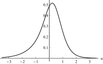
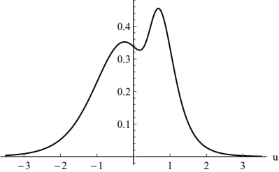
$f_{NM}$: $\frac{1}{5}N(-\frac{3}{4},1)+\frac{1}{5}N(-\frac{1}{4},(\frac{2}{3})^{2})+\frac{3}{5}N(\frac{1}{3},(\frac{5}{9})^{2})$	$f_{NM}$: $\frac{3}{4}N(-\frac{1}{3},1)+\frac{1}{4}N(1,(\frac{1}{3})^{2})$
$R(f^{(4)})^{-1/9}=0.595872$, $R(f^{(3)})^{-1/7}=0.738786$.	$R(f^{(4)})^{-1/9}=0.372818$, $R(f^{(3)})^{-1/7}=0.499502$.

Figure 1: Selected mixture densities (scaled)

5.3 Kernel Functions and Bandwidths

Fourth order Gaussian-based kernels, $k(x)=(3-x^{2})\phi(x)/2$ and $K(x)=\Phi(x)+x\phi(x)/2$, $\Phi(x)=\int_{-\infty}^{x}\phi(u)\mathrm{d}u$, are employed; see Wand and Schucany (1990, Section 2) and Oryshchenko (2017) respectively. Thus the choices of the asymptotically optimal bandwidths $(27/4\sqrt{\pi})^{1/9}R(f^{(4)})^{-1/9}n^{-1/9}$ and $(7/2\sqrt{\pi})^{1/7}R(f^{(3)})^{-1/7}n^{-1/7}$ for p.d.f. and c.d.f. estimation respectively are permitted, thereby satisfying Assumptions 3.4(c) and 4.1(b). The practical issue of estimating the derivatives of $f$ required for the computation of $R(f^{(j)})$, $j=3,4$, is ignored and the respective true values used. For the standard normal distribution these are $R(\phi^{(3)})=15/(16\sqrt{\pi})$ and $R(\phi^{(4)})=105/(32\sqrt{\pi})$; for the mixture distributions, approximate values are shown in Figure 1.

5.4 Results

The study compares the performance of GEL-based kernel density p.d.f. and c.d.f. estimators. The GEL parameter estimators are CUE, EL and ET, the most notable special cases of the GEL family. For each estimator the mean and variance were computed on a grid $1000$ of points between $-5$ and $5$ and are reported as the integrated squared bias and integrated variance relative to those of the corresponding infeasible estimator based on the true $u$, i.e., $\tilde{f}$ and $\widetilde{F}$.

Tables 1, 2 and 3 report results for Scenarios 1, 2 and 3 respectively. The ISB, IVar and MISE (all $\times 10^{5}$) for the infeasible $\tilde{f}$ and $\widetilde{F}$ are presented. Rows ISB, IVar, and MISE are the ISB, IVar, and MISE of $\hat{f}$, $\hat{f}_{\rho}$ ($\widehat{F}$, $\widehat{F}_{\rho}$) relative to the infeasible $\tilde{f}$ ($\widetilde{F}$), respectively; row ‘vs $d_{g}=3$’ is the MISE of $\hat{f}$, $\hat{f}_{\rho}$ ($\hat{F}$, $\widehat{F}_{\rho}$) relative to the corresponding value for $d_{g}=3$; row ‘w. vs unw.’ is the MISE of $\hat{f}_{\rho}$ ($\widehat{F}_{\rho}$) relative to $\hat{f}$ ($\widehat{F}$). Rows MISE, ‘vs $d_{g}=3$’, and ‘w. vs unw.’ examine the significance of the paired $t$-statistics in a two-sided test for equality of the respective ISE means, e.g., $\int(\hat{f}(u)-f(u))^{2}\mathrm{d}u$; the symbol † indicates that the $p$-value is between $0.01$ and $0.05$ whereas ‡ that it is less than $0.01$ and in all other cases the $p$-value is greater than $0.05$. Values of relative MISE less than $1$ are emphasised in bold.

Sample sizes $n=100$, $500$, $1000$, and $2000$ are examined.

All computations were carried out in MATLAB; the relevant code and additional results, including the properties of GEL estimators, are available from the first named author upon request. All results are based on $10,000$ random draws.

Table 1: Performance of GEL-based residual density and distribution function estimators in the IHS transformation model, $\operatorname{arsinh}(0.08y)/0.08=1+2x+u$, in Scenario 1

		$\tilde{f}$	$\widetilde{F}$	$d_{g}=3$		$d_{g}=4$				$d_{g}=5$
				$\hat{f}$	$\widehat{F}$	$\hat{f}$	$\hat{f}_{\rho}$	$\widehat{F}$	$\widehat{F}_{\rho}$	$\hat{f}$	$\hat{f}_{\rho}$	$\widehat{F}$	$\widehat{F}_{\rho}$
$n=100$
CUE	$\operatorname{ISB}$	31.3	8.9	0.70	3.41	0.13	0.20	0.47	1.12	0.12	0.37	0.56	1.85
	$\operatorname{IVar}$	449.0	402.3	1.29	0.71	0.88	0.88	0.46	0.43	0.87	0.86	0.47	0.42
	$\operatorname{MISE}$	480.2	411.2	1.26 ‡	0.78 ‡	0.83 ‡	0.83 ‡	0.46 ‡	0.45 ‡	0.82 ‡	0.83 ‡	0.47 ‡	0.45 ‡
vs $d_{g}=3$						0.66 ‡	0.66 ‡	0.60 ‡	0.58 ‡	0.65 ‡	0.66 ‡	0.61 ‡	0.59 ‡
w. vs unw.						0.999		0.965 ‡		1.010 ‡		0.964 ‡
[2pt/2pt]EL	$\operatorname{ISB}$					0.16	0.17	0.56	0.64	0.17	0.20	0.71	0.87
	$\operatorname{IVar}$					0.84	0.84	0.45	0.42	0.87	0.89	0.51	0.45
	$\operatorname{MISE}$					0.80 ‡	0.80 ‡	0.45 ‡	0.42 ‡	0.83 ‡	0.85 ‡	0.51 ‡	0.46 ‡
vs $d_{g}=3$						0.64 ‡	0.64 ‡	0.58 ‡	0.55 ‡	0.66 ‡	0.68 ‡	0.66 ‡	0.60 ‡
w. vs unw.						1.001		0.930 ‡		1.024		0.906 ‡
[2pt/2pt]ET	$\operatorname{ISB}$					0.15	0.20	0.55	1.01	0.14	0.34	0.66	1.70
	$\operatorname{IVar}$					0.83	0.89	0.43	0.47	0.85	0.86	0.48	0.53
	$\operatorname{MISE}$					0.79 ‡	0.85 ‡	0.44 ‡	0.48 ‡	0.81 ‡	0.84 ‡	0.49 ‡	0.88
vs $d_{g}=3$						0.63 ‡	0.68 ‡	0.56 ‡	0.62 ‡	0.64 ‡	0.67 ‡	0.64 ‡	1.16
w. vs unw.						1.071 †		1.092		1.037		1.789
$n=500$
CUE	$\operatorname{ISB}$	10.0	1.8	0.37	1.53	0.46	0.36	0.29	0.28	0.40	0.27	0.27	0.33
	$\operatorname{IVar}$	119.8	88.3	0.99	0.61	0.87	0.87	0.46	0.45	0.88	0.88	0.47	0.46
	$\operatorname{MISE}$	129.8	90.2	0.94 ‡	0.63 ‡	0.84 ‡	0.83 ‡	0.45 ‡	0.45 ‡	0.84 ‡	0.83 ‡	0.47 ‡	0.46 ‡
vs $d_{g}=3$						0.89 ‡	0.88 ‡	0.72 ‡	0.71 ‡	0.90 ‡	0.89 ‡	0.74 ‡	0.73 ‡
w. vs unw.						0.991 ‡		0.988 ‡		0.988 ‡		0.986 ‡
[2pt/2pt]EL	$\operatorname{ISB}$					0.45	0.45	0.29	0.30	0.41	0.40	0.28	0.29
	$\operatorname{IVar}$					0.87	0.87	0.46	0.45	0.88	0.88	0.47	0.46
	$\operatorname{MISE}$					0.83 ‡	0.84 ‡	0.45 ‡	0.45 ‡	0.84 ‡	0.84 ‡	0.47 ‡	0.46 ‡
vs $d_{g}=3$						0.89 ‡	0.89 ‡	0.72 ‡	0.72 ‡	0.89 ‡	0.90 ‡	0.74 ‡	0.73 ‡
w. vs unw.						1.002 ‡		0.993 ‡		1.003 †		0.979 ‡
[2pt/2pt]ET	$\operatorname{ISB}$					0.45	0.39	0.29	0.28	0.40	0.31	0.27	0.30
	$\operatorname{IVar}$					0.87	0.87	0.46	0.45	0.88	0.88	0.47	0.46
	$\operatorname{MISE}$					0.83 ‡	0.83 ‡	0.45 ‡	0.45 ‡	0.84 ‡	0.83 ‡	0.46 ‡	0.46 ‡
vs $d_{g}=3$						0.89 ‡	0.88 ‡	0.72 ‡	0.71 ‡	0.89 ‡	0.89 ‡	0.74 ‡	0.73 ‡
w. vs unw.						0.996 ‡		0.991 ‡		0.994 ‡		0.986 ‡
$n=1000$
CUE	$\operatorname{ISB}$	6.1	0.9	0.48	1.03	0.62	0.55	0.41	0.33	0.58	0.46	0.36	0.28
	$\operatorname{IVar}$	66.1	45.6	0.99	0.62	0.89	0.89	0.48	0.48	0.90	0.90	0.49	0.49
	$\operatorname{MISE}$	72.2	46.5	0.95 ‡	0.63 ‡	0.87 ‡	0.86 ‡	0.48 ‡	0.47 ‡	0.87 ‡	0.86 ‡	0.49 ‡	0.48 ‡
vs $d_{g}=3$						0.91 ‡	0.91 ‡	0.76 ‡	0.75 ‡	0.92 ‡	0.91 ‡	0.78 ‡	0.77 ‡
w. vs unw.						0.992 ‡		0.990 ‡		0.988 ‡		0.988 ‡
[2pt/2pt]EL	$\operatorname{ISB}$					0.62	0.62	0.40	0.40	0.59	0.58	0.37	0.36
	$\operatorname{IVar}$					0.89	0.89	0.48	0.48	0.89	0.89	0.49	0.48
	$\operatorname{MISE}$					0.86 ‡	0.86 ‡	0.48 ‡	0.48 ‡	0.87 ‡	0.87 ‡	0.49 ‡	0.48 ‡
vs $d_{g}=3$						0.91 ‡	0.91 ‡	0.76 ‡	0.76 ‡	0.91 ‡	0.91 ‡	0.77 ‡	0.77 ‡
w. vs unw.						1.001 †		0.996 ‡		1.001		0.989 ‡
[2pt/2pt]ET	$\operatorname{ISB}$					0.62	0.58	0.40	0.36	0.58	0.50	0.36	0.30
	$\operatorname{IVar}$					0.89	0.89	0.48	0.48	0.89	0.89	0.49	0.48
	$\operatorname{MISE}$					0.86 ‡	0.86 ‡	0.48 ‡	0.47 ‡	0.87 ‡	0.86 ‡	0.48 ‡	0.48 ‡
vs $d_{g}=3$						0.91 ‡	0.91 ‡	0.76 ‡	0.76 ‡	0.91 ‡	0.91 ‡	0.77 ‡	0.76 ‡
w. vs unw.						0.996 ‡		0.993 ‡		0.993 ‡		0.990 ‡
$n=2000$
CUE	$\operatorname{ISB}$	3.5	0.4	0.55	0.62	0.74	0.69	0.53	0.45	0.71	0.62	0.49	0.37
	$\operatorname{IVar}$	36.6	23.0	1.02	0.65	0.92	0.92	0.52	0.52	0.93	0.93	0.53	0.52
	$\operatorname{MISE}$	40.1	23.5	0.98 ‡	0.65 ‡	0.90 ‡	0.90 ‡	0.52 ‡	0.51 ‡	0.91 ‡	0.90 ‡	0.53 ‡	0.52 ‡
vs $d_{g}=3$						0.92 ‡	0.92 ‡	0.80 ‡	0.79 ‡	0.93 ‡	0.92 ‡	0.81 ‡	0.80 ‡
w. vs unw.						0.994 ‡		0.994 ‡		0.990 ‡		0.992 ‡
[2pt/2pt]EL	$\operatorname{ISB}$					0.74	0.74	0.52	0.52	0.71	0.71	0.48	0.48
	$\operatorname{IVar}$					0.92	0.92	0.52	0.52	0.92	0.92	0.52	0.52
	$\operatorname{MISE}$					0.90 ‡	0.90 ‡	0.52 ‡	0.52 ‡	0.90 ‡	0.90 ‡	0.52 ‡	0.52 ‡
vs $d_{g}=3$						0.92 ‡	0.92 ‡	0.80 ‡	0.80 ‡	0.92 ‡	0.93 ‡	0.81 ‡	0.80 ‡
w. vs unw.						1.000		0.999		1.001		0.996 ‡
[2pt/2pt]ET	$\operatorname{ISB}$					0.74	0.71	0.53	0.48	0.71	0.65	0.49	0.41
	$\operatorname{IVar}$					0.92	0.92	0.52	0.52	0.92	0.92	0.52	0.52
	$\operatorname{MISE}$					0.90 ‡	0.90 ‡	0.52 ‡	0.52 ‡	0.90 ‡	0.90 ‡	0.52 ‡	0.52 ‡
vs $d_{g}=3$						0.92 ‡	0.92 ‡	0.80 ‡	0.79 ‡	0.93 ‡	0.92 ‡	0.80 ‡	0.80 ‡
w. vs unw.						0.997 ‡		0.996 ‡		0.994 ‡		0.994 ‡

Notes: see text.

Table 2: Performance of GEL-based residual density and distribution function estimators in the IHS transformation model, $\operatorname{arsinh}(0.08y)/0.08=1+2x+u$, in Scenario 2

		$\tilde{f}$	$\widetilde{F}$	$d_{g}=3$		$d_{g}=4$				$d_{g}=5$
				$\hat{f}$	$\widehat{F}$	$\hat{f}$	$\hat{f}_{\rho}$	$\widehat{F}$	$\widehat{F}_{\rho}$	$\hat{f}$	$\hat{f}_{\rho}$	$\widehat{F}$	$\widehat{F}_{\rho}$
$n=100$
CUE	$\operatorname{ISB}$	29.3	3.8	0.73	5.71	0.85	1.13	2.65	5.14	0.99	1.52	3.65	7.65
	$\operatorname{IVar}$	822.0	427.7	1.12	0.75	0.93	0.94	0.54	0.50	0.93	0.94	0.55	0.49
	$\operatorname{MISE}$	852.5	432.5	1.11 ‡	0.79 ‡	0.93 ‡	0.94 ‡	0.56 ‡	0.54 ‡	0.93 ‡	0.95 ‡	0.57 ‡	0.55 ‡
vs $d_{g}=3$						0.84 ‡	0.85 ‡	0.70 ‡	0.68 ‡	0.84 ‡	0.86 ‡	0.72 ‡	0.70 ‡
w. vs unw.						1.013 ‡		0.963 ‡		1.026 ‡		0.966 ‡
[2pt/2pt]EL	$\operatorname{ISB}$					0.71	0.78	1.95	2.59	0.70	0.83	1.99	3.03
	$\operatorname{IVar}$					0.92	0.93	0.53	0.50	0.93	0.96	0.56	0.51
	$\operatorname{MISE}$					0.91 ‡	0.93 ‡	0.54 ‡	0.52 ‡	0.92 ‡	0.95 ‡	0.57 ‡	0.54 ‡
vs $d_{g}=3$						0.82 ‡	0.84 ‡	0.68 ‡	0.66 ‡	0.83 ‡	0.86 ‡	0.72 ‡	0.68 ‡
w. vs unw.						1.015 ‡		0.956 ‡		1.029 ‡		0.934 ‡
[2pt/2pt]ET	$\operatorname{ISB}$					0.77	0.97	2.37	4.19	0.86	1.28	2.99	6.22
	$\operatorname{IVar}$					0.91	0.95	0.51	0.59	0.92	0.94	0.55	0.63
	$\operatorname{MISE}$					0.90 ‡	0.95	0.53 ‡	0.62 ‡	0.92 ‡	0.96	0.58 ‡	0.80
vs $d_{g}=3$						0.82 ‡	0.86 ‡	0.67 ‡	0.80	0.83 ‡	0.87 ‡	0.73 ‡	1.03
w. vs unw.						1.054 †		1.174		1.053 ‡		1.390
$n=500$
CUE	$\operatorname{ISB}$	10.0	0.8	0.80	4.25	0.88	0.86	0.96	1.36	0.87	0.84	1.15	1.92
	$\operatorname{IVar}$	210.2	89.9	1.08	0.82	0.93	0.93	0.53	0.52	0.93	0.93	0.53	0.51
	$\operatorname{MISE}$	220.4	90.9	1.07 ‡	0.85 ‡	0.93 ‡	0.93 ‡	0.54 ‡	0.52 ‡	0.93 ‡	0.93 ‡	0.54 ‡	0.53 ‡
vs $d_{g}=3$						0.87 ‡	0.87 ‡	0.63 ‡	0.62 ‡	0.87 ‡	0.87 ‡	0.63 ‡	0.62 ‡
w. vs unw.						1.001		0.980 ‡		1.001		0.980 ‡
[2pt/2pt]EL	$\operatorname{ISB}$					0.87	0.89	0.87	0.94	0.84	0.85	0.86	0.98
	$\operatorname{IVar}$					0.93	0.98	0.53	0.72	0.93	0.93	0.53	0.52
	$\operatorname{MISE}$					0.93 ‡	0.97	0.53 ‡	0.72	0.92 ‡	0.93 ‡	0.53 ‡	0.52 ‡
vs $d_{g}=3$						0.87 ‡	0.91 †	0.63 ‡	0.85	0.87 ‡	0.87 ‡	0.63 ‡	0.62 ‡
w. vs unw.						1.049		1.343		1.005 ‡		0.978 ‡
[2pt/2pt]ET	$\operatorname{ISB}$					0.88	0.87	0.93	1.16	0.85	0.82	1.03	1.50
	$\operatorname{IVar}$					0.93	0.93	0.53	0.52	0.92	0.93	0.52	0.51
	$\operatorname{MISE}$					0.93 ‡	0.93 ‡	0.53 ‡	0.52 ‡	0.92 ‡	0.92 ‡	0.53 ‡	0.52 ‡
vs $d_{g}=3$						0.87 ‡	0.87 ‡	0.63 ‡	0.62 ‡	0.86 ‡	0.87 ‡	0.62 ‡	0.61 ‡
w. vs unw.						1.001 ‡		0.982 ‡		1.002 ‡		0.984 ‡
$n=1000$
CUE	$\operatorname{ISB}$	6.5	0.5	0.84	2.78	0.94	0.92	0.89	0.99	0.91	0.87	0.94	1.19
	$\operatorname{IVar}$	115.0	45.7	1.09	0.81	0.94	0.94	0.54	0.53	0.94	0.94	0.54	0.52
	$\operatorname{MISE}$	121.7	46.3	1.07 ‡	0.83 ‡	0.94 ‡	0.94 ‡	0.54 ‡	0.53 ‡	0.94 ‡	0.94 ‡	0.54 ‡	0.53 ‡
vs $d_{g}=3$						0.88 ‡	0.88 ‡	0.65 ‡	0.64 ‡	0.88 ‡	0.87 ‡	0.65 ‡	0.64 ‡
w. vs unw.						0.999 ‡		0.982 ‡		0.999 ‡		0.980 ‡
[2pt/2pt]EL	$\operatorname{ISB}$					0.94	0.95	0.87	0.89	0.92	0.92	0.84	0.88
	$\operatorname{IVar}$					0.94	0.94	0.54	0.53	0.94	0.94	0.54	0.53
	$\operatorname{MISE}$					0.94 ‡	0.94 ‡	0.54 ‡	0.54 ‡	0.94 ‡	0.94 ‡	0.54 ‡	0.53 ‡
vs $d_{g}=3$						0.88 ‡	0.88 ‡	0.65 ‡	0.64 ‡	0.87 ‡	0.88 ‡	0.65 ‡	0.64 ‡
w. vs unw.						1.001 ‡		0.982 ‡		1.003 ‡		0.984 ‡
[2pt/2pt]ET	$\operatorname{ISB}$					0.94	0.93	0.88	0.93	0.91	0.88	0.89	1.01
	$\operatorname{IVar}$					0.94	0.94	0.54	0.53	0.94	0.94	0.53	0.52
	$\operatorname{MISE}$					0.94 ‡	0.94 ‡	0.54 ‡	0.53 ‡	0.94 ‡	0.94 ‡	0.54 ‡	0.53 ‡
vs $d_{g}=3$						0.88 ‡	0.88 ‡	0.65 ‡	0.64 ‡	0.87 ‡	0.87 ‡	0.65 ‡	0.63 ‡
w. vs unw.						1.000		0.982 ‡		1.000		0.983 ‡
$n=2000$
CUE	$\operatorname{ISB}$	4.2	0.3	0.93	1.88	0.99	0.97	0.96	0.97	0.96	0.92	0.94	1.01
	$\operatorname{IVar}$	64.9	23.7	1.09	0.81	0.95	0.95	0.55	0.54	0.95	0.95	0.55	0.54
	$\operatorname{MISE}$	69.1	24.0	1.08 ‡	0.82 ‡	0.95 ‡	0.95 ‡	0.56 ‡	0.55 ‡	0.95 ‡	0.95 ‡	0.55 ‡	0.54 ‡
vs $d_{g}=3$						0.88 ‡	0.88 ‡	0.68 ‡	0.67 ‡	0.88 ‡	0.87 ‡	0.68 ‡	0.66 ‡
w. vs unw.						0.999 ‡		0.983 ‡		0.998 ‡		0.979 ‡
[2pt/2pt]EL	$\operatorname{ISB}$					0.99	0.99	0.95	0.95	0.97	0.97	0.91	0.93
	$\operatorname{IVar}$					0.95	0.95	0.56	0.55	0.95	0.95	0.55	0.54
	$\operatorname{MISE}$					0.95 ‡	0.95 ‡	0.56 ‡	0.55 ‡	0.95 ‡	0.95 ‡	0.56 ‡	0.54 ‡
vs $d_{g}=3$						0.88 ‡	0.88 ‡	0.68 ‡	0.67 ‡	0.88 ‡	0.88 ‡	0.68 ‡	0.66 ‡
w. vs unw.						1.000		0.983 ‡		1.000		0.978 ‡
[2pt/2pt]ET	$\operatorname{ISB}$					0.99	0.98	0.96	0.95	0.95	0.93	0.92	0.94
	$\operatorname{IVar}$					0.95	0.95	0.55	0.54	0.95	0.95	0.55	0.54
	$\operatorname{MISE}$					0.95 ‡	0.95 ‡	0.56 ‡	0.55 ‡	0.95 ‡	0.94 ‡	0.55 ‡	0.54 ‡
vs $d_{g}=3$						0.88 ‡	0.88 ‡	0.68 ‡	0.67 ‡	0.87 ‡	0.87 ‡	0.67 ‡	0.66 ‡
w. vs unw.						0.999 ‡		0.983 ‡		0.999 ‡		0.980 ‡

Notes: see text.

Table 3: Performance of GEL-based residual density and distribution function estimators in the IHS transformation model, $\operatorname{arsinh}(0.08y)/0.08=1+2x+u$, in Scenario 3

		$\tilde{f}$	$\widetilde{F}$	$d_{g}=3$		$d_{g}=4$				$d_{g}=5$
				$\hat{f}$	$\widehat{F}$	$\hat{f}$	$\hat{f}_{\rho}$	$\widehat{F}$	$\widehat{F}_{\rho}$	$\hat{f}$	$\hat{f}_{\rho}$	$\widehat{F}$	$\widehat{F}_{\rho}$
$n=100$
CUE	$\operatorname{ISB}$	23.9	1.3	7.34	41.60	4.25	5.01	14.61	24.59	4.68	6.19	17.12	33.44
	$\operatorname{IVar}$	1546.0	485.4	1.19	0.76	1.01	1.01	0.53	0.50	1.01	1.02	0.55	0.50
	$\operatorname{MISE}$	1570.5	487.0	1.28 ‡	0.88 ‡	1.06 ‡	1.08 ‡	0.57 ‡	0.56 ‡	1.07 ‡	1.10 ‡	0.59 ‡	0.59 ‡
vs $d_{g}=3$						0.82 ‡	0.84 ‡	0.65 ‡	0.65 ‡	0.83 ‡	0.86 ‡	0.67 ‡	0.68 ‡
w. vs unw.						1.018 ‡		0.986 ‡		1.033 ‡		0.999
[2pt/2pt]EL	$\operatorname{ISB}$					4.08	4.08	13.99	15.96	4.28	4.38	13.51	17.07
	$\operatorname{IVar}$					0.99	1.01	0.51	0.49	1.00	1.04	0.54	0.51
	$\operatorname{MISE}$					1.04 ‡	1.05 ‡	0.55 ‡	0.53 ‡	1.05 ‡	1.09 ‡	0.57 ‡	0.55 ‡
vs $d_{g}=3$						0.81 ‡	0.82 ‡	0.62 ‡	0.61 ‡	0.82 ‡	0.85 ‡	0.65 ‡	0.64 ‡
w. vs unw.						1.014 ‡		0.972 ‡		1.034 ‡		0.972
[2pt/2pt]ET	$\operatorname{ISB}$					4.14	4.71	14.22	22.01	4.53	5.69	14.89	27.85
	$\operatorname{IVar}$					0.99	1.01	0.50	0.49	1.00	1.02	0.66	0.84
	$\operatorname{MISE}$					1.03 ‡	1.06 ‡	0.54 ‡	0.54 ‡	1.05 ‡	1.09 ‡	0.78	1.91
vs $d_{g}=3$						0.81 ‡	0.83 ‡	0.62 ‡	0.62 ‡	0.82 ‡	0.85 ‡	0.90	2.25
w. vs unw.						1.027 ‡		1.006		1.040 ‡		2.459
$n=500$
CUE	$\operatorname{ISB}$	9.6	0.4	2.39	13.99	1.54	1.58	2.61	3.94	1.60	1.69	2.84	5.19
	$\operatorname{IVar}$	379.2	100.3	1.10	0.76	1.00	1.00	0.51	0.50	1.00	1.00	0.51	0.50
	$\operatorname{MISE}$	388.9	100.8	1.13 ‡	0.81 ‡	1.01 ‡	1.01 ‡	0.52 ‡	0.51 ‡	1.01 ‡	1.02 ‡	0.52 ‡	0.51 ‡
vs $d_{g}=3$						0.89 ‡	0.90 ‡	0.64 ‡	0.63 ‡	0.90 ‡	0.90 ‡	0.65 ‡	0.64 ‡
w. vs unw.						1.002 ‡		0.981 ‡		1.004 ‡		0.982 ‡
[2pt/2pt]EL	$\operatorname{ISB}$					1.54	1.55	2.55	2.65	1.57	1.59	2.46	2.59
	$\operatorname{IVar}$					1.00	1.00	0.51	0.50	1.00	1.07	0.51	0.80
	$\operatorname{MISE}$					1.01 ‡	1.01 ‡	0.51 ‡	0.50 ‡	1.01 ‡	1.09	0.52 ‡	0.81
vs $d_{g}=3$						0.89 ‡	0.89 ‡	0.64 ‡	0.62 ‡	0.89 ‡	0.96	0.64 ‡	1.00
w. vs unw.						1.002 ‡		0.979 ‡		1.074		1.563
[2pt/2pt]ET	$\operatorname{ISB}$					1.53	1.56	2.59	3.40	1.58	1.64	2.65	4.11
	$\operatorname{IVar}$					1.00	1.00	0.51	0.49	1.00	1.00	0.50	0.49
	$\operatorname{MISE}$					1.01 ‡	1.01 ‡	0.51 ‡	0.50 ‡	1.01 ‡	1.01 ‡	0.51 ‡	0.51 ‡
vs $d_{g}=3$						0.89 ‡	0.89 ‡	0.64 ‡	0.62 ‡	0.89 ‡	0.90 ‡	0.64 ‡	0.63 ‡
w. vs unw.						1.002 ‡		0.982 ‡		1.004 ‡		0.985 ‡
$n=1000$
CUE	$\operatorname{ISB}$	6.6	0.2	1.86	8.15	1.33	1.34	1.66	2.16	1.37	1.39	1.80	2.79
	$\operatorname{IVar}$	206.9	50.4	1.09	0.74	1.00	1.00	0.51	0.50	1.00	1.00	0.51	0.50
	$\operatorname{MISE}$	213.5	50.6	1.12 ‡	0.77 ‡	1.01 ‡	1.01 ‡	0.52 ‡	0.51 ‡	1.01 ‡	1.01 ‡	0.52 ‡	0.51 ‡
vs $d_{g}=3$						0.90 ‡	0.90 ‡	0.67 ‡	0.66 ‡	0.91 ‡	0.91 ‡	0.67 ‡	0.66 ‡
w. vs unw.						1.001 ‡		0.980 ‡		1.001 ‡		0.978 ‡
[2pt/2pt]EL	$\operatorname{ISB}$					1.34	1.35	1.65	1.64	1.36	1.37	1.68	1.74
	$\operatorname{IVar}$					1.00	1.13	0.51	1.09	1.00	1.00	0.51	0.50
	$\operatorname{MISE}$					1.01 ‡	1.14	0.52 ‡	1.09	1.01 ‡	1.01 ‡	0.52 ‡	0.50 ‡
vs $d_{g}=3$						0.90 ‡	1.02	0.67 ‡	1.41	0.90 ‡	0.90 ‡	0.67 ‡	0.65 ‡
w. vs unw.						1.124		2.108		1.001 †		0.973 ‡
[2pt/2pt]ET	$\operatorname{ISB}$					1.34	1.34	1.66	1.91	1.36	1.37	1.76	2.32
	$\operatorname{IVar}$					1.00	1.00	0.51	0.50	1.00	1.00	0.51	0.49
	$\operatorname{MISE}$					1.01 ‡	1.01 ‡	0.51 ‡	0.50 ‡	1.01 ‡	1.01 ‡	0.51 ‡	0.50 ‡
vs $d_{g}=3$						0.90 ‡	0.90 ‡	0.67 ‡	0.65 ‡	0.90 ‡	0.90 ‡	0.66 ‡	0.65 ‡
w. vs unw.						1.001 ‡		0.979 ‡		1.001 ‡		0.979 ‡
$n=2000$
CUE	$\operatorname{ISB}$	4.0	0.1	1.60	4.53	1.24	1.23	1.34	1.54	1.25	1.25	1.41	1.86
	$\operatorname{IVar}$	113.2	25.6	1.10	0.74	1.00	1.00	0.52	0.51	1.00	1.00	0.52	0.51
	$\operatorname{MISE}$	117.2	25.8	1.11 ‡	0.76 ‡	1.01 ‡	1.01 ‡	0.53 ‡	0.52 ‡	1.01 ‡	1.01 ‡	0.52 ‡	0.51 ‡
vs $d_{g}=3$						0.91 ‡	0.91 ‡	0.69 ‡	0.68 ‡	0.91 ‡	0.91 ‡	0.69 ‡	0.67 ‡
w. vs unw.						0.999 ‡		0.981 ‡		0.999 ‡		0.977 ‡
[2pt/2pt]EL	$\operatorname{ISB}$					1.25	1.25	1.34	1.35	1.25	1.26	1.36	1.38
	$\operatorname{IVar}$					1.00	1.00	0.52	0.51	1.00	1.11	0.52	0.91
	$\operatorname{MISE}$					1.01 ‡	1.01 ‡	0.53 ‡	0.52 ‡	1.01 ‡	1.12	0.53 ‡	0.92
vs $d_{g}=3$						0.91 ‡	0.91 ‡	0.69 ‡	0.68 ‡	0.91 ‡	1.00	0.69 ‡	1.20
w. vs unw.						0.999 ‡		0.980 ‡		1.105		1.743
[2pt/2pt]ET	$\operatorname{ISB}$					1.24	1.24	1.34	1.43	1.24	1.25	1.39	1.62
	$\operatorname{IVar}$					1.00	1.00	0.52	0.51	1.00	1.00	0.52	0.51
	$\operatorname{MISE}$					1.01 ‡	1.01 ‡	0.53 ‡	0.52 ‡	1.01 ‡	1.01 ‡	0.52 ‡	0.51 ‡
vs $d_{g}=3$						0.91 ‡	0.91 ‡	0.69 ‡	0.68 ‡	0.91 ‡	0.91 ‡	0.69 ‡	0.67 ‡
w. vs unw.						0.999 ‡		0.980 ‡		0.999 ‡		0.977 ‡

Notes: see text.

5.4.1 Scenario 1

The first $\sim b$ term in eq. (5.2) is approximately $-0.321n^{-1/9}$, which for $n=100$, $500$, $1000$, and $2000$ is approximately $-0.192$, $-0.161$, $-0.149$, and $-0.138$ respectively. The second $\sim b$ term is approximately $0.04728n^{-1/9}$ for $d_{g}=4$ and $0.04708n^{-1/9}$ for $d_{g}=5$, which offsets the reduction in variance slightly. The predicted relative IVar of $\hat{f}$ and $\hat{f}_{\rho}$ up to order $\mathit{o}(b)$ is thus $0.836$, $0.863$, $0.873$ and $0.882$ for $n=100$, $500$, $1000$, and $2000$ respectively and is identical within three digit precision for $d_{g}=4$ and $5$.

The results reported in Table 1 confirm these predictions. In fact, the reduction in variance is even larger than expected in small and medium samples due to the $\mathit{o}(b)$ effects. Furthermore, estimators $\hat{f}$ and $\hat{f}_{\rho}$ have smaller ISB relative to $\tilde{f}$. A comparison of $\hat{f}$ and $\hat{f}_{\rho}$ between $d_{g}=3$ (just-identified) and $d_{g}=4,5$ (over-identified) for moderate and larger sample sizes emphasises further the contribution of additional moment information. Hence $\hat{f}$ and $\hat{f}_{\rho}$ enjoy a reduction in MISE of as much as $21\%$ for $n=100$ and $10\%$ for $n=2000$ relative to $\tilde{f}$. The benefits are even more pronounced for c.d.f. estimation, where the reduction in MISE can be as much as $56\%$ for $n=100$ and around $53\%$ in moderate samples. There are also small but statistically significant benefits to re-weighting which are mostly due to the smaller biases of $\hat{f}_{\rho}$ and $\widehat{F}_{\rho}$ relative to $\hat{f}$ and $\widehat{F}$ at moderate and larger sample sizes. There is some deterioration in ISB, IVar and, thus, MISE with increases in $d_{g}$ which can be contributed to the increased importance of outliers.

Finally, while in moderate and large samples the performances of CUE, EL, and ET are virtually identical, in small samples ET can be unstable with larger $d_{g}$.

5.4.2 Scenarios 2 and 3

Scenarios 2 and 3 with densities of $(x,u)$ which are heavy-tailed and also, e.g., skewed and bimodal, illustrate the many difficulties for both GEL estimation and kernel p.d.f. and c.d.f. estimation which are absent in the relatively benign Scenario 1.

The performance of CUE in small samples is generally worse than that of EL and ET. It ranks last by MSE in both scenarios with $n=100$ and $500$, except Scenario 3 with $n=100$ where ET underperforms. In a number of cases increasing with $d_{g}$ the optimisation routine for ET failed. Somewhat surprisingly, although it is known to be sensitive to outliers, EL appears to deliver good results in the simulation experiments. It ranks first by MSE in Scenario 3 with $d_{g}=5$ and alternates with ET otherwise. These differences become very small with $n=1,000$ and greater.

The conclusion about the inferior performance of CUE in small samples holds true for CUE-based kernel density p.d.f. and c.d.f. estimators as well; see Tables 2 and 3, in particular, the ISBs of $\hat{f}$ and $\hat{f}_{\rho}$ with $d_{g}=4,5$ in Table 2. However, the ranking of EL and ET-based kernel density p.d.f. and c.d.f. estimators by MISE does not always correspond to the ranking of the underlying EL and ET estimators of $\beta_{0}$ by MSE. In particular, the sensitivity of EL to outliers adversely affects the estimators $\hat{f}_{\rho}$ and $\widehat{F}_{\rho}$ via the implied probabilities in Scenario 3 with $n=500$ and greater; see Table 3. ET and CUE perform better in those cases.

Unlike Scenario 1, in Scenario 3 none of the feasible kernel density estimators have smaller MISE than their infeasible counterparts for the sample sizes considered. In Scenario 2, with less complicated distributional features, these estimators do achieve a reduction in MISE with $d_{g}=4,5$. The same is true for the feasible kernel c.d.f. estimators in Scenario 2 with $d_{g}=3,4,5$, and more often than not in Scenario 3 as well, with the few exceptions mentioned above. Importantly, it is generally beneficial to increase the number of moment conditions beyond those necessary to identify the parameters except when stability of GEL estimators of $\beta_{0}$ is likely to deteriorate.

Finally, the benefits of re-weighting are present, but not universal, and as expected, are quite small; cf. Supplement LABEL:Supp:Examples: Example B.4.

6 Summary and Conclusions

Large sample results and simulation evidence reported in this paper suggest that it is generally sensible to apply either the standard or re-weighted kernel estimators to estimate the p.d.f. or c.d.f. of a scalar residual $u(z,\beta_{0})$ in a variety of situations, provided error associated with the estimation of $\beta_{0}$ satisfies some mild regularity conditions and care is taken to ensure the bandwidth is not too small. If the assumptions on $u(z,\beta)$ prove difficult to verify in practice, using fourth or higher order kernels and the corresponding asymptotically optimal bandwidths will generally assist with ensuring the appropriate regularity conditions hold.

Incorporating information from overidentifying moment conditions by re-weighting the estimators using GEL implied probabilities offers efficiency gains which are realised in regular situations. However, if the model is highly nonlinear and the distribution of the data is heavy-tailed or contaminated with outliers, the methods proposed in this paper, including GEL, should be applied with some caution in very small samples. Robustified hybrid estimators such as the exponentially tilted empirical likelihood, see, e.g., Schennach (2007), may prove useful in these circumstances.

While the results in this paper were presented only for the scalar-valued $u(z,\beta)$, generalisations to the vector case are relatively straightforward provided an analogue of the bijection Assumption 3.1 holds.

An issue for future research to usefully address is the construction of tests for overidentifying moment conditions or parametric restrictions based on the differences between the kernel p.d.f. estimators $\hat{f}_{\rho}$ and $\hat{f}$ or $\tilde{f}_{\rho}$ and $\tilde{f}$ for known $\beta_{0}$. Test statistics of the Bickel-Rosenblatt type based on the integrated squared difference $\int(\hat{f}_{\rho}(u)-\hat{f}(u))^{2}\mathrm{d}u$, Bickel and Rosenblatt (1973), Fan (1994, 1998), or the integrated absolute difference, Cao and Lugosi (2005), would be of interest. Alternatively, Kolmogorov-Smirnov or Cramér-von Mises-type tests could be constructed based on the differences between kernel c.d.f. estimators.

Supplement A to “Improved Density and Distribution Function Estimation”: Proofs Vitaliy Oryshchenko^* Richard J. Smith Department of Economics cemmap, U.C.L and I.F.S. University of Manchester Faculty of Economics, University of Cambridge Department of Economics, University of Melbourne ONS Economic Statistics Centre of Excellence

A

Throughout the Appendix, $0<C<\infty$ and $0\leq\omega\leq 1$ will denote generic constants that may be different in different uses. CS, T, and H refer to the Cauchy-Schwarz, triangle, and Hölder inequalities, respectively with LIE and WLLN the law of iterated expectations and Khintchine’s i.i.d. weak law of large numbers. MVT is the mean value theorem.

In addition, $\mathop{\mathrm{int}}(\cdot)$ denotes the interior of $\cdot$, w.p.(a.)1 with probability (approaching) 1, and $\mathcal{N}$ is an open neighbourhood of $\beta_{0}$.

A.1 GEL Stochastic Expansions

The following identification and regularity conditions are imposed.

Assumption A.1.

(a) $\beta_{0}\in\mathcal{B}$ is the unique solution to $\operatorname{E}[g(z,\beta)]=0$; (b) $\mathcal{B}$ is compact; (c) $g(z,\beta)$ is continuous at each $\beta\in\mathcal{B}$ w.p.1; (d) $\operatorname{E}[\sup_{\beta\in\mathcal{B}}\lVert g(z,\beta)\rVert^{2}]<\infty$; (e) $\Omega$ is nonsingular; (f) $\rho(v)$ is twice continuously differentiable in a neighbourhood of zero.

Assumption A.1 is Newey and Smith (2004, Assumption 1) and is sufficient for the consistency of $\hat{\beta}$. Moreover, $\hat{\lambda}=\operatorname*{argmax}_{\lambda\in\Lambda_{n}(\hat{\beta})}P_{n}(\hat{\beta},\lambda)$ exists w.p.a.1 and $\hat{\lambda}=\mathit{O}_{p}(n^{-1/2})$; see Newey and Smith (2004, Theorem 3.1).

Assumption A.2.

(a) $\beta_{0}\in\mathop{\mathrm{int}}(\mathcal{B})$; (b) $g(z,\beta)$ is continuously differentiable for $\beta\in\mathcal{N}$ and
$\operatorname{E}[\sup_{\beta\in\mathcal{N}}\lVert\nabla g(z,\beta)\rVert]<\infty$; (c) $\mathop{\mathrm{rank}}(G)=d_{\beta}$.

Assumption A.2 is Newey and Smith (2004, Assumption 2). If Assumptions A.1 and A.2 hold then $n^{1/2}((\hat{\beta}-\beta_{0})^{\top},\>\hat{\lambda}^{\top})^{\top}\xrightarrow{d}N\left(0,\mathop{\mathrm{diag}}(\Sigma,P)\right)$; see Newey and Smith (2004, Theorem 3.2).

Let $\nabla^{2}g(z,\beta)$ denote a vector of all distinct second order partial derivatives with respect to $\beta$.

Assumption A.3.

(a) $\operatorname{E}[\lVert g(z,\beta_{0})\rVert^{6}]<\infty$; (b) $g(z,\beta)$ is twice differentiable for $\beta\in\mathcal{N}$, $\operatorname{E}[\lVert\nabla g(z,\beta_{0})\rVert^{4}]$ $<\infty$, $\operatorname{E}[\lVert\nabla^{2}g(z,\beta_{0})\rVert^{2}]<\infty$; (c) there exists $d(z)\geq 0$ with $\operatorname{E}[d(z)^{2}]<\infty$ such that $\lVert\nabla^{2}g(z,\beta)-\nabla^{2}g(z,\beta_{0})\rVert\leq d(z)\lVert\beta-\beta_{0}\rVert$ for all $z$ and $\beta\in\mathcal{N}$; (d) $\rho(v)$ is four times differentiable with Lipschitz fourth derivative in a neighbourhood of zero.

Cf. Newey and Smith (2004, Assumption 3).

Write $\tilde{g}=n^{-1}\sum_{i=1}^{n}g_{i}$, $\widetilde{G}=n^{-1}\sum_{i=1}^{n}G_{i}-G$, and $\widetilde{\Omega}=n^{-1}\sum_{i=1}^{n}g_{i}g_{i}^{\top}-\Omega$. Also let $g_{i}^{j}=\partial g(z_{i},\beta_{0})/\partial\beta_{j}$ and $G_{i}^{j}=\partial^{2}g(z_{i},\beta_{0})/\partial\beta_{j}\partial\beta^{\top}$, $j=1,\ldots,d_{\beta}$. From the proof of Theorem 3.4 in Newey and Smith (2004), GEL estimators satisfy the following stochastic expansion

$$\begin{bmatrix}\hat{\beta}-\beta_{0}\\ \hat{\lambda}\end{bmatrix}=-\begin{bmatrix}H\\ P\end{bmatrix}\tilde{g}+\begin{bmatrix}-\Sigma&H\\ H^{\top}&P\end{bmatrix}\tilde{\zeta}+\mathit{O}_{p}(n^{-3/2}),$$ (A.1)

where

$$\tilde{\zeta} =\left\{\begin{bmatrix}0&\widetilde{G}^{\top}\\ \widetilde{G}&\widetilde{\Omega}\end{bmatrix}-\frac{1}{2}\sum_{j=1}^{d_{\beta}}[H\tilde{g}]_{j}\begin{bmatrix}0&E[G_{i}^{j}]^{\top}\\ E[G_{i}^{j}]&E[g_{i}^{j}g_{i}^{\top}+g_{i}g_{i}^{j\top}]\end{bmatrix}\right.$$

$$\qquad\left.-\frac{1}{2}\sum_{j=1}^{d_{g}}[P\tilde{g}]_{j}\begin{bmatrix}E[\partial^{2}g_{ij}/\partial\beta\partial\beta^{\top}]&E[G_{i}^{\top}e_{j}g_{i}^{\top}+g_{ij}G_{i}^{\top}]\\ E[g_{i}e_{j}^{\top}G_{i}+g_{ij}G_{i}]&-\rho_{3}E[g_{ij}g_{i}g_{i}^{\top}]\end{bmatrix}\right\}\begin{bmatrix}H\\ P\end{bmatrix}\tilde{g}.$$

Remark A.1.

Write $\tilde{\zeta}=(\tilde{\zeta}_{\beta}^{\top},\tilde{\zeta}_{\lambda}^{\top})^{\top}$ partitioned conformably with $\beta$ and $\lambda$. Then $\operatorname{E}[\tilde{\zeta}_{\beta}]=0$ and $\operatorname{E}[\tilde{\zeta}_{\lambda}]=\zeta_{\lambda}$ given in eq. (2.2). If $\beta_{0}$ is known, the stochastic expansion for $\tilde{\lambda}$ is identical to that in eq. (A.1) except $H$ is set to zero and $\Omega^{-1}$ replaces $P$, i.e., $\tilde{\lambda}=-\Omega^{-1}\tilde{g}+\Omega^{-1}\tilde{\zeta}_{\lambda}+\mathit{O}_{p}(n^{-3/2})$, where $\tilde{\zeta}_{\lambda}=\widetilde{\Omega}\Omega^{-1}\tilde{g}+\rho_{3}\sum_{j=1}^{d_{\beta}}[\Omega^{-1}\tilde{g}]_{j}\operatorname{E}[g_{ij}g_{i}g_{i}^{\top}]\Omega^{-1}\tilde{g}/2$. Thus, in expectation, the first two terms in eq. (2.2) are eliminated and $\operatorname{E}[\tilde{\zeta}_{\lambda}]=n^{-1}c_{\rho}\operatorname{E}[g_{i}g_{i}^{\top}\Omega^{-1}g_{i}]$.

Remark A.2.

When $\beta_{0}$ is known, Assumptions A.3(b,c) can be relaxed to $g(z,\beta)$ is continuously differentiable for $\beta\in\mathcal{N}$, $\operatorname{E}[\sup_{\beta\in\mathcal{N}}\lVert\nabla g(z,\beta_{0})\rVert]<\infty$, and there exists $d(z)\geq 0$ with $\operatorname{E}[d(z)]<\infty$ such that $\lVert\nabla g(z,\beta)-\nabla g(z,\beta_{0})\rVert\leq d(z)\lVert\beta-\beta_{0}\rVert$ for all $z$ and $\beta\in\mathcal{N}$. The Lipschitz condition in Assumptions A.3(b,c,d) can also be relaxed to $\alpha$-Hölder for some $0<\alpha\leq 1$ and changing the remainder terms from $\mathit{O}(n^{-3/2})$ to $\mathit{O}(n^{-1-\alpha/2})$.

Remark A.3.

The two-step GMM estimator is defined as $\hat{\beta}_{GMM}=\operatorname*{argmin}_{\beta\in\mathcal{B}}\hat{g}(\beta)^{\top}\widehat{\Omega}(\tilde{\beta})^{-1}\hat{g}(\beta)$ where $\tilde{\beta}$ is a $\sqrt{n}$-consistent preliminary estimator of $\beta_{0}$. If the preliminary estimator $\tilde{\beta}$ is first order efficient, i.e., $\tilde{\beta}-\beta_{0}=-H\tilde{g}+\mathit{O}_{p}(n^{-1})$, then, if Assumptions A.1–A.3 hold, all GMM estimators $\hat{\beta}_{GMM}$ admit the same expansion to order $\mathit{O}_{p}(n^{-3/2})$; see Newey and Smith (2004, Section 3). Moreover, defining $\hat{\lambda}_{GMM}=-\widehat{\Omega}(\tilde{\beta})^{-1}\hat{g}(\hat{\beta}_{GMM})$, the expansion is

$$\begin{bmatrix}\hat{\beta}_{GMM}-\beta_{0}\\ \hat{\lambda}_{GMM}\end{bmatrix}=-\begin{bmatrix}H\\ P\end{bmatrix}\tilde{g}+\begin{bmatrix}-\Sigma&H\\ H^{\top}&P\end{bmatrix}\tilde{\zeta}^{GMM}+\mathit{O}_{p}(n^{-3/2}),$$

where

$$\tilde{\zeta}^{GMM} =\left\{\begin{bmatrix}0&\widetilde{G}^{\top}\\ \widetilde{G}&\widetilde{\Omega}-\sum_{j=1}^{d_{\beta}}\operatorname{E}[g_{i}^{j}g_{i}^{\top}+g_{i}g_{i}^{j\top}]e_{j}^{\top}H\tilde{g}\end{bmatrix}-\frac{1}{2}\sum_{j=1}^{d_{\beta}}[H\tilde{g}]_{j}\begin{bmatrix}0&E[G_{i}^{j}]^{\top}\\ E[G_{i}^{j}]&0\end{bmatrix}\right.$$

$$\qquad\left.-\frac{1}{2}\sum_{j=1}^{d_{g}}[P\tilde{g}]_{j}\begin{bmatrix}E[\partial^{2}g_{ij}/\partial\beta\partial\beta^{\top}]&0\\ 0&0\end{bmatrix}\right\}\begin{bmatrix}H\\ P\end{bmatrix}\tilde{g}.$$

Writing $\tilde{\zeta}^{GMM}=(\tilde{\zeta}_{\beta}^{GMM\top},\tilde{\zeta}_{\lambda}^{GMM\top})^{\top}$ partitioned conformably with $\beta$ and $\lambda$, $\zeta_{\beta}^{GMM}=\operatorname{E}[\tilde{\zeta}_{\beta}^{GMM}]=\operatorname{E}[G_{i}^{\top}Pg_{i}]$ and $\zeta_{\lambda}^{GMM}=\operatorname{E}[\tilde{\zeta}_{\lambda}]=-a+\operatorname{E}[G_{i}Hg_{i}]+\operatorname{E}[g_{i}g_{i}^{\top}Pg_{i}]$. Hence, the second order bias of $\hat{\beta}_{GMM}$, Newey and Smith (2004, Theorem 4.2), is given by

$$\operatorname{E}[\hat{\beta}_{GMM}]-\beta_{0}=-n^{-1}\Sigma\zeta_{\beta}^{GMM}+n^{-1}H\zeta_{\lambda}^{GMM}+\mathit{O}(n^{-3/2}),$$

the notable difference with GEL being the additional term $-n^{-1}\Sigma\zeta_{\beta}^{GMM}$ with the term $n^{-1}H\zeta_{\lambda}^{GMM}$ identical to CUE.

A.2 Preliminary Lemmas

Lemma A.1.

If Assumptions A.1–A.3 are satisfied, then

$$n\hat{\pi}_{i}=1-g_{i}^{\top}P\tilde{g}-\tfrac{\rho_{3}}{2}(g_{i}^{\top}P\tilde{g})^{2}+g_{i}^{\top}\begin{bmatrix}H^{\top}&P\end{bmatrix}\tilde{\zeta}+\tilde{g}^{\top}PG_{i}H\tilde{g}+c_{\rho}\tilde{g}^{\top}P\tilde{g}+\mathit{o}_{p}(n^{-1})$$ (A.1)

uniformly $i=1,\ldots,n$.

Proof. Let $\hat{v}_{i}=\hat{\lambda}^{\top}g(z_{i},\hat{\beta})$. A third order Taylor expansion of $\rho^{(1)}(\hat{v}_{i})$ around $0$ yields

$$\rho^{(1)}(\hat{v}_{i})=-1-\hat{v}_{i}+\tfrac{\rho_{3}}{2}\hat{v}_{i}^{2}+\tfrac{\rho_{4}}{6}\hat{v}_{i}^{3}(1+\mathit{o}_{p}(1))$$

noting $\lvert\hat{v}_{i}\rvert\xrightarrow{p}0$ uniformly $i=1,\ldots,n$ by Newey and Smith (2004, Lemma A1). A Taylor expansion from eq. (A.1) of $g(z_{i},\hat{\beta})$ about $\beta_{0}$ yields $g(z_{i},\hat{\beta})=g_{i}-G_{i}H\tilde{g}+\mathit{o}_{p}(n^{-1/2})$ uniformly $i=1,\ldots,n$ by Owen (1990, Lemma 3). Hence, substituting, using eq. (A.1),

$$\rho^{(1)}(\hat{v}_{i})=-1+g_{i}^{\top}P\tilde{g}-g_{i}^{\top}\begin{bmatrix}H^{\top}&P\end{bmatrix}\tilde{\zeta}-\tilde{g}^{\top}H^{\top}G_{i}^{\top}P\tilde{g}+\tfrac{\rho_{3}}{2}(g_{i}^{\top}P\tilde{g})^{2}+\mathit{o}_{p}(n^{-1}).$$

From a similar expansion, using $n^{-1}\sum_{i=1}^{n}g(z_{i},\hat{\beta})=\Omega P\tilde{g}+\mathit{O}_{p}(n^{-1})$, eq. (A.1), and $P\Omega P=P$,

$$n^{-1}{\textstyle\sum}_{i=1}^{n}\rho^{(1)}(\hat{v}_{i})=-1-\hat{\lambda}^{\top}\Omega P\tilde{g}+\tfrac{\rho_{3}}{2}\hat{\lambda}^{\top}\Omega\hat{\lambda}+\mathit{O}_{p}(n^{-3/2})=-1+c_{\rho}\tilde{g}^{\top}P\tilde{g}+\mathit{O}_{p}(n^{-3/2}).$$

Hence, $[{\textstyle\sum}_{i=1}^{n}\rho^{(1)}(\hat{v}_{i})]^{-1}=-n^{-1}[1+c_{\rho}\tilde{g}^{\top}P\tilde{g}+\mathit{O}_{p}(n^{-3/2})]$ and

$$n\hat{\pi}_{i}=1-g_{i}^{\top}P\tilde{g}+g_{i}^{\top}\begin{bmatrix}H^{\top}&P\end{bmatrix}\tilde{\zeta}+\tilde{g}^{\top}H^{\top}G_{i}^{\top}P\tilde{g}-\tfrac{\rho_{3}}{2}(g_{i}^{\top}P\tilde{g})^{2}+c_{\rho}\tilde{g}^{\top}P\tilde{g}+\mathit{o}_{p}(n^{-1})$$

uniformly $i=1,\ldots,n$. $\blacksquare$

Corollary A.1.(Known $\beta_{0}$)

If Assumptions A.1–A.3 are satisfied, then

$$n\tilde{\pi}_{i}=1-g_{i}^{\top}\Omega^{-1}\tilde{g}-\tfrac{\rho_{3}}{2}(g_{i}^{\top}\Omega^{-1}\tilde{g})^{2}+g_{i}^{\top}\Omega^{-1}\tilde{\zeta}_{\lambda}+c_{\rho}\tilde{g}^{\top}\Omega^{-1}\tilde{g}+\mathit{o}_{p}(n^{-1})$$ (A.2)

uniformly $i=1,\ldots,n$.

Let $a(z)$ denote a real scalar function of $z$ such that $\operatorname{E}[a(z)^{2}]<\infty$. Write $a_{i}=a(z_{i})$, $i=1,\ldots,n$.

Lemma A.2.

If Assumptions A.1–A.3 are satisfied, then

$$\operatorname{E}[(n\hat{\pi}_{i}-1)a_{i}]=n^{-1}\left(-c_{\rho}\operatorname{E}[a_{i}g_{i}^{\top}Pg_{i}]+\operatorname{E}[a_{i}g_{i}^{\top}]P\zeta_{\lambda}+c_{\rho}(d_{g}-d_{\beta})\operatorname{E}[a_{i}]\right)+\mathit{o}(n^{-1})$$ (A.3)

uniformly $i=1,\ldots,n$. For $i\neq j$,

$$\operatorname{E}[(n\hat{\pi}_{i}-1)a_{i}a_{j}]=\operatorname{E}[(n\hat{\pi}_{i}-1)a_{i}]\operatorname{E}[a_{j}]-n^{-1}\operatorname{E}[a_{i}g_{i}^{\top}]P\operatorname{E}[g_{j}a_{j}]+\mathit{O}(n^{-2}),$$ (A.4)

$$\operatorname{E}[(n\hat{\pi}_{i}-1)(n\hat{\pi}_{j}-1)a_{i}a_{j}]=n^{-1}\operatorname{E}[a_{i}g_{i}^{\top}]P\operatorname{E}[g_{j}a_{j}]+\mathit{O}(n^{-2}).$$ (A.5)

Let $\bar{a}=n^{-1}\sum_{i=1}^{n}a_{i}$ and $\hat{a}=\sum_{i=1}^{n}\hat{\pi}_{i}a_{i}$. Then,

$$\operatorname{Var}[\hat{a}]=\operatorname{Var}[\bar{a}]-n^{-1}\operatorname{E}[a_{i}g_{i}^{\top}]P\operatorname{E}[g_{j}a_{j}]+\mathit{O}(n^{-2}).$$ (A.6)

Proof. The first result follows from the expansion for $\hat{\pi}_{i}$ in Lemma A.1. In particular, noting $\operatorname{E}[g_{i}]=0$ and $\operatorname{E}[a_{i}\mathit{o}_{p}(n^{-1})]=\mathit{o}(n^{-1})$ by uniformity of $\mathit{o}_{p}(n^{-1})$, then, by independence,

$$\operatorname{E}[(n\hat{\pi}_{i}-1)a_{i}] =-n^{-1}\operatorname{E}[a_{i}g_{i}^{\top}Pg_{i}]-\tfrac{\rho_{3}}{2}n^{-1}\operatorname{E}[a_{i}g_{i}^{\top}P\operatorname{E}[g_{j}g_{j}^{\top}]Pg_{i}]+\operatorname{E}[a_{i}g_{i}^{\top}]\begin{bmatrix}H^{\top}&P\end{bmatrix}\operatorname{E}[\tilde{\zeta}]$$

$$\quad+n^{-1}\mathop{\mathrm{tr}}(\operatorname{E}[a_{i}G_{i}]H\operatorname{E}[g_{j}g_{j}^{\top}]P)+c_{\rho}n^{-1}\operatorname{E}[a_{i}]\mathop{\mathrm{tr}}(\operatorname{E}[g_{j}g_{j}^{\top}]P)+\mathit{o}(n^{-1})$$

$$=-n^{-1}c_{\rho}\operatorname{E}[a_{i}g_{i}^{\top}Pg_{i}]+n^{-1}\operatorname{E}[a_{i}g_{i}^{\top}]P\zeta_{\lambda}+n^{-1}c_{\rho}(d_{g}-d_{\beta})\operatorname{E}[a_{i}]+\mathit{o}(n^{-1})$$

uniformly $i=1,\ldots,n$, using $\operatorname{E}[\tilde{\zeta}]=(0^{\top},n^{-1}\zeta_{\lambda}^{\top})^{\top}$, $P\Omega P=P$, $H\Omega P=0$, and $\mathop{\mathrm{tr}}(\Omega P)=d_{g}-d_{\beta}$. Eqs. (A.4) and (A.5) follow by a similar argument.

Finally note that $\hat{a}-\bar{a}=n^{-1}\sum_{i=1}^{n}(n\hat{\pi}_{i}-1)a_{i}$. Hence, $\operatorname{Var}[\hat{a}]=\operatorname{Var}[\bar{a}]+\operatorname{Var}[\hat{a}-\bar{a}]+2\operatorname{Cov}[\hat{a}-\bar{a},\bar{a}]$. Now, from above, $\operatorname{E}[\hat{a}-\bar{a}]=\mathit{O}(n^{-1})$. Hence,

$$\operatorname{Var}[\hat{a}-\bar{a}]=\operatorname{E}_{i\neq j}[(n\hat{\pi}_{i}-1)(n\hat{\pi}_{j}-1)a_{i}a_{j}]+\mathit{O}(n^{-2})=n^{-1}\operatorname{E}[a_{i}g_{i}^{\top}]P\operatorname{E}[g_{j}a_{j}]+\mathit{O}(n^{-2}).$$

Also,

$$\operatorname{Cov}[\hat{a}-\bar{a},\xi] =n^{-1}\operatorname{E}[(n\hat{\pi}_{i}-1)a_{i}^{2}]+(1-n^{-1})\operatorname{E}_{i\neq j}[(n\hat{\pi}_{i}-1)a_{i}a_{j}]-\operatorname{E}[(n\hat{\pi}_{i}-1)a_{i})]E[a_{j}]$$

$$=-n^{-1}\operatorname{E}[a_{i}g_{i}^{\top}]P\operatorname{E}[g_{j}a_{j}]+\mathit{O}(n^{-2}). \blacksquare$$

Corollary A.2.(Known $\beta_{0}$)

If Assumptions A.1–A.3 are satisfied, then

$$\operatorname{E}[(n\tilde{\pi}_{i}-1)a_{i}]=n^{-1}c_{\rho}\left(-\operatorname{E}[g_{i}^{\top}\Omega^{-1}g_{i}a_{i}]+\operatorname{E}[g_{i}^{\top}\Omega^{-1}g_{i}g_{i}^{\top}]\Omega^{-1}\operatorname{E}[g_{i}a_{i}]+q\operatorname{E}[a_{i}]\right)+\mathit{o}(n^{-1})$$ (A.7)

uniformly $i=1,\ldots,n$. Lemma A.2 remains valid with $\Omega^{-1}$ replacing $P$.

Repeated use is made of the following lemma; see Bochner (1955, Theorem 1.1.1) and Parzen (1962, Theorem 1A). See also Pagan and Ullah (1999, App.A.2.6).

Lemma A.3.

Suppose that $f:\mathbbm{R}\mapsto\mathbbm{R}$ and $k:\mathbbm{R}\mapsto\mathbbm{R}$ are Borel functions satisfying (a) $\int_{-\infty}^{\infty}\lvert f(x)\rvert\mathrm{d}x<\infty$; (b) $\sup_{-\infty<x<\infty}\lvert k(x)\rvert<\infty$, $\int_{-\infty}^{\infty}\lvert k(x)\rvert\mathrm{d}x<\infty$, and $\lim_{\lvert x\rvert\to\infty}\lvert xk(x)\rvert=0$. Then ${\textstyle\int}_{-\infty}^{\infty}b^{-1}\lvert k((y-x)/b)\rvert\lvert f(x)\rvert\mathrm{d}x<\infty$ a.e. and

$$\lim_{b\downarrow 0}\lvert{\textstyle\int}_{-\infty}^{\infty}b^{-1}k((y-x)/b)f(x)\mathrm{d}x-f(y){\textstyle\int}_{-\infty}^{\infty}k(t)\mathrm{d}t\rvert=0$$ (A.8)

at every continuity point $y$ of $f$; if $f$ is uniformly continuous, then convergence is uniform. Under the same conditions $\lim_{b\downarrow 0}\lvert\int_{-\infty}^{\infty}b^{-1}k((y-x)/b)^{r}f(x)\mathrm{d}x-f(y)\int_{-\infty}^{\infty}k(t)^{r}\mathrm{d}t\rvert=0$ at every continuity point $y$ of $f$ for any $r\geq 1$. If $\sup_{-\infty<x<\infty}\lvert f(x)\rvert<\infty$, $\int_{-\infty}^{\infty}\lvert k(x)\rvert\mathrm{d}x<\infty$ is sufficient for (A.8) to hold. $\square$

Remark A.1.

If $k$ is Hölder continuous with exponent $0<\tau\leq 1$ and, thus, uniformly continuous, and absolutely integrable, then it is bounded.

A.3 Proofs of Theorems

Proof of Theorem 3.1. Write $\tilde{f}_{\rho}(u)=\tilde{f}(u)+n^{-1}\sum_{i=1}^{n}(n\tilde{\pi}_{i}-1)k_{b}(u-u_{i})$. By Corollary A.1 and Owen (1990, Lemma 3), $\max_{1\leq i\leq n}\lvert n\tilde{\pi}_{i}-1\rvert=\mathit{o}_{p}(1)$. By Lemma A.3, $\operatorname{E}[\lvert k_{b}(u-u_{i})\rvert]<\infty$ whenever $\lvert f(u)\rvert<\infty$ which holds a.e. Thus, $k_{b}(u-u_{i})$, $i=1,\ldots,n$, satisfies the conditions for WLLN. Hence, the first conclusion follows.

From Assumption 3.2(a)(i), $b\operatorname{E}[k_{b}(u-u_{i})^{2}]<\infty$ a.e. By CS, invoking Assumptions A.1(e) and A.3(a), $\operatorname{E}[\lvert g_{i}b^{1/2}k_{b}(u-u_{i})\rvert]<\infty$ and $\operatorname{E}[\lvert g_{i}^{\top}\Omega^{-1}g_{i}b^{1/2}k_{b}(u-u_{i})\rvert]<\infty$. Hence, by Corollary A.2, setting $a_{i}=b^{1/2}k_{b}(u-u_{i})$,

$$\operatorname{E}[(n\tilde{\pi}_{i}-1)k_{b}(u-u_{i})]=n^{-1}c_{\rho}\{ -\operatorname{E}[g_{i}^{\top}\Omega^{-1}g_{i}k_{b}(u-u_{i})]+\operatorname{E}[g_{i}^{\top}\Omega^{-1}g_{i}g_{i}^{\top}]\Omega^{-1}\operatorname{E}[g_{i}k_{b}(u-u_{i})]$$

$$+d_{g}\operatorname{E}[k_{b}(u-u_{i})]\}+\mathit{o}(n^{-1}).$$

Under Assumption 3.2(a)(i), $\operatorname{E}[k_{b}(u-u_{i})]=f(u)+\mathit{o}(1)$. Invoking Assumption 3.1 and the change of variables $z\mapsto(u,v^{\top})^{\top}$, then, by LIE and Lemma A.3, $\operatorname{E}[g_{i}k_{b}(u-u_{i})]=\int\operatorname{E}[g_{i}|t]f(t)k_{b}(u-t)\mathrm{d}t=\operatorname{E}[g_{i}|u]f(u)+\mathit{o}(1)$. Similarly, $\operatorname{E}[g_{i}^{\top}\Omega^{-1}g_{i}k_{b}(u-u_{i})]=\operatorname{E}[g_{i}^{\top}\Omega^{-1}g_{i}|u]f(u)+\mathit{o}(1)$. The final result is a direct consequence of Lemma A.2 and the same argument. $\blacksquare$

Set

$$\hat{\delta}_{1}(u) =n^{-1}{\textstyle\sum}_{i=1}^{n}\left[k_{b}(u-\hat{u}_{i})-k_{b}(u-u_{i})\right];$$ (A.1)

$$\hat{\delta}_{2}(u) =n^{-1}{\textstyle\sum}_{i=1}^{n}(n\hat{\pi}_{i}-1)\left[k_{b}(u-\hat{u}_{i})-k_{b}(u-u_{i})\right];$$ (A.2)

$$\hat{\delta}_{3}(u) =n^{-1}{\textstyle\sum}_{i=1}^{n}(n\hat{\pi}_{i}-1)k_{b}(u-u_{i}).$$ (A.3)

Note $\hat{f}(u)=\tilde{f}(u)+\hat{\delta}_{1}(u)$ and $\hat{f}_{\rho}(u)=\hat{f}(u)+\hat{\delta}_{2}(u)+\hat{\delta}_{3}(u)$.

Proof of Theorem 3.2. Under Assumptions A.1 and A.2, $\hat{\beta}\in\mathcal{N}$ w.p.a.1 and $n^{1/2}(\hat{\beta}-\beta_{0})=\mathit{O}_{p}(1)$. First, by Assumption 3.3(a,b), from eq. (A.1),

$$\lvert\hat{\delta}_{1}(u)\rvert \leq\tfrac{1}{n}{\textstyle\sum}_{i=1}^{n}\lvert k_{b}(u-\hat{u}_{i})-k_{b}(u-u_{i})\rvert\leq\tfrac{C}{nb^{1+\tau}}{\textstyle\sum}_{i=1}^{n}\lvert\hat{u}_{i}-u_{i}\rvert^{\tau}$$

$$\leq\tfrac{C}{n^{\alpha\tau/2}b^{1+\tau}}\lVert n^{1/2}(\hat{\beta}-\beta_{0})\rVert^{\alpha\tau}\tfrac{1}{n}{\textstyle\sum}_{i=1}^{n}d(z_{i})^{\tau}=\mathit{o}_{p}(1)$$

since $n^{-1}\sum_{i=1}^{n}d(z_{i})^{\tau}=\mathit{O}_{p}(1)$ by WLLN and $n^{\alpha\tau/2}b^{1+\tau}\to\infty$ from Assumption 3.3(c). Next, $\max_{1\leq i\leq n}\lvert n\hat{\pi}_{i}-1\rvert=\mathit{o}_{p}(1)$ by Lemma A.1 and Owen (1990, Lemma 3), from eq. (A.2),

$$\lvert\hat{\delta}_{2}(u)\rvert \leq\tfrac{1}{n}{\textstyle\sum}_{i=1}^{n}\lvert(n\hat{\pi}_{i}-1)\left[k_{b}(u-\hat{u}_{i})-k_{b}(u-u_{i})\right]\rvert$$

$$\leq\tfrac{C}{n^{\alpha\tau/2}b^{1+\tau}}\lVert n^{1/2}(\hat{\beta}-\beta_{0})\rVert^{\alpha\tau}(\max_{1\leq i\leq n}\lvert n\hat{\pi}_{i}-1\rvert)\tfrac{1}{n}{\textstyle\sum}_{i=1}^{n}d(z_{i})^{\tau}=\mathit{o}_{p}(1).$$

Hence, the first conclusion follows. The final result follows from eq. (A.3), by noting that also

$$\lvert\hat{\delta}_{3}(u)\rvert\leq\tfrac{1}{n}{\textstyle\sum}_{i=1}^{n}\lvert(n\hat{\pi}_{i}-1)k_{b}(u-u_{i})\rvert\leq(\max_{1\leq i\leq n}\lvert n\hat{\pi}_{i}-1\rvert)\tfrac{1}{n}{\textstyle\sum}_{i=1}^{n}\lvert k_{b}(u-u_{i})\rvert=\mathit{o}_{p}(1)$$

by WLLN since $\operatorname{E}[\lvert k_{b}(u-u_{i})\rvert]<\infty$ a.e. by Lemma A.3. $\blacksquare$

Proof of Theorem 3.3. Preliminaries. From a second order Taylor expansion around $\beta_{0}$,

$$k_{b}(u-\hat{u}_{i}) =k_{b}(u-u_{i})-k_{b}^{(1)}(u-u_{i})\nabla^{\top}u_{i}(\hat{\beta}-\beta_{0})$$

$$+\tfrac{1}{2}(\hat{\beta}-\beta_{0})^{\top}[k_{b}^{(2)}(u-\bar{u}_{i})\nabla\bar{u}_{i}\nabla^{\top}\bar{u}_{i}-k_{b}^{(1)}(u-\bar{u}_{i})\nabla^{2}\bar{u}_{i}](\hat{\beta}-\beta_{0}),$$

where $k_{b}^{(j)}(x)=k^{(j)}(x/b)/b^{j+1}$, $j=1,2$, and $\bar{u}_{i}=u(z_{i},\bar{\beta})$, $i=1,\ldots,n$, with $\bar{\beta}$ on the line segment joining $\hat{\beta}$ and $\beta_{0}$; and $\nabla\bar{u}_{i}$ and $\nabla^{2}\bar{u}_{i}$, $i=1,\ldots,n$, are defined analogously. Note that $\lVert\bar{\beta}-\beta_{0}\rVert\leq\lVert\hat{\beta}-\beta_{0}\rVert=\mathit{O}_{p}(n^{-1/2})$. Assumption 3.4(b) and twice differentiability of $u(z,\beta)$ for $\beta\in\mathcal{N}$ implies there exist $d_{0}(z)\geq 0$ with $\operatorname{E}[d_{0}(z)^{4}]<\infty$ and $d_{1}(z)\geq 0$ with $\operatorname{E}[d_{1}(z)^{4}]<\infty$ such that $\lvert u(z,\beta)-u(z,\beta_{0})\rvert\leq d_{0}(z)\lVert\beta-\beta_{0}\rVert$ and $\lVert\nabla u(z,\beta)-\nabla u(z,\beta_{0})\rVert\leq d_{1}(z)\lVert\beta-\beta_{0}\rVert$ for all $z$ and $\beta\in\mathcal{N}$. Thus, by T, $\lVert\nabla\bar{u}_{i}\nabla^{\top}\bar{u}_{i}-\nabla u_{i}\nabla^{\top}u_{i}\rVert\leq 2d_{1}(z_{i})\lVert\nabla u_{i}\rVert\lVert\hat{\beta}-\beta_{0}\rVert+d_{1}(z_{i})^{2}\lVert\hat{\beta}-\beta_{0}\rVert^{2}$. By Owen (1990, Lemma 3), $\max_{1\leq i\leq n}d_{1}(z_{i})^{2}=\mathit{o}_{p}(n^{1/2})$ and $\max_{1\leq i\leq n}d_{1}(z_{i})\lVert\nabla u_{i}\rVert=\mathit{o}_{p}(n^{1/2})$. Hence, $\lVert\nabla\bar{u}_{i}\nabla^{\top}\bar{u}_{i}-\nabla u_{i}\nabla^{\top}u_{i}\rVert\leq n^{-1/2}[d_{1}(z_{i})\lVert\nabla u_{i}\rVert+\mathit{o}_{p}(1)]\mathit{O}_{p}(1)$. By CS, from Assumption 3.4(b), for $0<\tau\leq 1$, $\operatorname{E}[d_{0}(z_{i})^{\tau}\lVert\nabla u_{i}\rVert^{2}]<\infty$ and $\operatorname{E}[d_{1}(z_{i})^{2}\lVert\nabla u_{i}\rVert^{2}]<\infty$. Thus, $\operatorname{E}[\lvert b^{-1/2}k^{(2)}((u-u_{i})/b)\rvert d_{1}(z_{i})\lVert\nabla u_{i}\rVert]<\infty$ since $\operatorname{E}[b^{-1}k^{(2)}((u-u_{i})/b)^{2}]<\infty$ also by CS and using Lemma A.3. Hence, by T, and noting $n^{\tau/2}b^{3+\tau}\to\infty$, $0<\tau\leq 1$, from Assumption 3.4(c),

$$\lVert\tfrac{1}{n}{\textstyle\sum}_{i=1}^{n}(k_{b}^{(2)}(u-\bar{u}_{i})\nabla\bar{u}_{i}\nabla^{\top}\bar{u}_{i}-k_{b}^{(2)}(u-u_{i})\nabla u_{i}\nabla^{\top}u_{i})\rVert$$

$$\qquad\leq\tfrac{C}{n^{\tau/2}b^{3+\tau}}\lVert n^{1/2}(\hat{\beta}-\beta_{0})\rVert^{\tau}\tfrac{1}{n}{\textstyle\sum}_{i=1}^{n}d_{0}(z_{i})^{\tau}\lVert\nabla u_{i}\rVert^{2}$$

$$\qquad\quad+\tfrac{1}{n}{\textstyle\sum}_{i=1}^{n}\left[\tfrac{1}{n^{1/2}b^{5/2}}\lvert b^{-1/2}k^{(2)}((u-u_{i})/b)\rvert+\tfrac{\mathit{o}_{p}(1)}{n^{\tau/2}b^{3+\tau}}\right]\left[d_{1}(z_{i})\lVert\nabla u_{i}\rVert+\mathit{o}_{p}(1)\right]\mathit{O}_{p}(1)=\mathit{o}_{p}(1).$$

Assumption 3.4(a) implies $k^{(1)}$ is Lipschitz, and hence, invoking Assumption 3.4(b), for all mean values $\bar{\beta}$ between $\hat{\beta}$ and $\beta_{0}$, $\lvert k_{b}^{(1)}(u-\bar{u}_{i})-k_{b}^{(1)}(u-u_{i})\rvert\leq b^{-3}Cd_{0}(z_{i})\lVert\hat{\beta}-\beta_{0}\rVert$ w.p.a.1. By Assumption 3.4(a) and Lemma A.3, $\operatorname{E}[b^{-1}|k^{(1)}((u-u_{i})/b)|^{4/3}]<\infty$ a.e., and as $\operatorname{E}[d(z_{i})^{4}]<\infty$, $\operatorname{E}[\lvert b^{-3/4}k^{(1)}((u-u_{i})/b)\rvert d(z_{i})]<\infty$ using the Hölder inequality with exponents $4/3$ and $4$. Therefore, by the same argument as above,

$$\lVert\tfrac{1}{n}{\textstyle\sum}_{i=1}^{n}(k_{b}^{(1)}(u-\bar{u}_{i})\nabla^{2}\bar{u}_{i}-k_{b}^{(1)}(u-u_{i})\nabla^{2}u_{i})\rVert\leq\tfrac{C}{n^{1/2}b^{3}}\lVert n^{1/2}(\hat{\beta}-\beta_{0})\rVert\tfrac{1}{n}{\textstyle\sum}_{i=1}^{n}d_{0}(z_{i})\lVert\nabla^{2}u_{i}\rVert$$

$$+\tfrac{1}{n^{\alpha/2}b^{5/4}}\lVert n^{1/2}(\hat{\beta}-\beta_{0})\rVert^{\alpha}\tfrac{1}{n}{\textstyle\sum}_{i=1}^{n}\left[\lvert b^{-3/4}k^{(1)}((u-u_{i})/b)\rvert+\tfrac{C}{n^{1/2}b^{7/4}}d_{0}(z_{i})\lVert n^{1/2}(\hat{\beta}-\beta_{0})\rVert\right]d(z_{i})=\mathit{o}_{p}(1).$$

Using expansion eq. (A.1) and Lemma A.1 eq. (A.1), from eq. (A.1),

$$\hat{\delta}_{1}(u) =\tfrac{1}{n}{\textstyle\sum}_{i=1}^{n}k_{b}^{(1)}(u-u_{i})\nabla^{\top}u_{i}H\tilde{g}-\tfrac{1}{n}{\textstyle\sum}_{i=1}^{n}k_{b}^{(1)}(u-u_{i})\nabla^{\top}u_{i}\begin{bmatrix}-\Sigma&H\end{bmatrix}\tilde{\zeta}$$

$$\quad+\tfrac{1}{2}\tilde{g}^{\top}H^{\top}\tfrac{1}{n}{\textstyle\sum}_{i=1}^{n}[k_{b}^{(2)}(u-u_{i})\nabla u_{i}\nabla^{\top}u_{i}-k_{b}^{(1)}(u-u_{i})\nabla^{2}u_{i}]H\tilde{g}+\mathit{o}_{p}(n^{-1}),$$ (A.4)

from eq. (A.2),

$$\hat{\delta}_{2}(u)=-\tfrac{1}{n}{\textstyle\sum}_{i=1}^{n}k_{b}^{(1)}(u-u_{i})\nabla^{\top}u_{i}H\tilde{g}\tilde{g}^{\top}Pg_{i}+\mathit{o}_{p}(n^{-1}),$$ (A.5)

and, from eq. (A.3),

$$\hat{\delta}_{3}(u) =\tfrac{1}{n}{\textstyle\sum}_{i=1}^{n}[-g_{i}^{\top}P\tilde{g}-\tfrac{\rho_{3}}{2}(g_{i}^{\top}P\tilde{g})^{2}+g_{i}^{\top}\begin{bmatrix}H^{\top}&P\end{bmatrix}\tilde{\zeta}+\tilde{g}^{\top}PG_{i}H\tilde{g}+c_{\rho}\tilde{g}^{\top}P\tilde{g}]k_{b}(u-u_{i})$$

$$\mkern 580.0mu+\mathit{o}_{p}(n^{-1}).$$ (A.6)

Expectation. Since $H\Omega H^{\top}=\Sigma$, from eq. (A.4),

$$\operatorname{E}[\hat{\delta}_{1}(u)] =n^{-1}\operatorname{E}[k_{b}^{(1)}(u-u_{i})\nabla^{\top}u_{i}Hg_{i}]-n^{-1}\operatorname{E}[k_{b}^{(1)}(u-u_{i})\nabla^{\top}u_{i}]H\zeta_{\lambda}$$

$$\quad+\tfrac{1}{2}n^{-1}\mathop{\mathrm{tr}}\left(\Sigma\operatorname{E}[k_{b}^{(2)}(u-u_{i})\nabla u_{i}\nabla^{\top}u_{i}-k_{b}^{(1)}(u-u_{i})\nabla^{2}u_{i}]\right)+\mathit{o}(n^{-1}).$$

Assumption 3.4(a) states $\lim_{\lvert x\rvert\to\infty}\lvert x^{2}k^{(1)}(x)\rvert=0$ and implies that $\int k^{(1)}(x)\mathrm{d}x=0$, $\int xk^{(1)}(x)\mathrm{d}x=-1$, and $xk^{(1)}(x)$ satisfies the hypotheses of Lemma A.3, i.e., it is bounded and absolutely integrable. Thus, invoking Assumption 3.4(d), by MVT and Lemma A.3,

$$\operatorname{E}[k_{b}^{(1)}(u-u_{i})\nabla u_{i}] =\tfrac{1}{b}{\textstyle\int}\operatorname{E}[\nabla u_{i}|u-bt]f(u-bt)k^{(1)}(t)\mathrm{d}t$$

$$=\tfrac{1}{b}\operatorname{E}[\nabla u_{i}|u]f(u){\textstyle\int}k^{(1)}(t)\mathrm{d}t-{\textstyle\int}(\mathrm{d}\{\operatorname{E}[\nabla u_{i}|u-\omega bt]f(u-\omega bt)\}/\mathrm{d}u)tk^{(1)}(t)\mathrm{d}t$$

$$=\mathrm{d}\{\operatorname{E}[\nabla u_{i}|u]f(u)\}/\mathrm{d}u+\mathit{o}(1).$$ (A.7)

Similarly, $\operatorname{E}[k_{b}^{(1)}(u-u_{i})\nabla^{\top}u_{i}Hg_{i}]=\mathrm{d}\{\operatorname{E}[\nabla^{\top}u_{i}Hg_{i}|u]f(u)\}/\mathrm{d}u+\mathit{o}(1)$ and $\operatorname{E}[k_{b}^{(1)}(u-u_{i})\nabla^{2}u_{i}]=\mathrm{d}\{\operatorname{E}[\nabla^{2}u_{i}|u]f(u)\}/\mathrm{d}u+\mathit{o}(1)$. Furthermore, Assumption 3.4(a) also implies that $\int k^{(2)}(x)\mathrm{d}x=0$, $\int xk^{(2)}(x)\mathrm{d}x=0$, $\int x^{2}k^{(2)}(x)\mathrm{d}x=2$, and $x^{2}k^{(2)}(x)$ satisfies the hypotheses of Lemma A.3. Thus, by a second order Taylor expansion and a similar argument to eq. (A.7),

$$\operatorname{E}[k_{b}^{(2)}(u-u_{i})\nabla u_{i}\nabla^{\top}u_{i}] =\tfrac{1}{b^{2}}{\textstyle\int}\operatorname{E}[\nabla u_{i}\nabla^{\top}u_{i}|u-bt]f(u-bt)k^{(2)}(t)\mathrm{d}t$$

$$=\tfrac{1}{b^{2}}\operatorname{E}[\nabla u_{i}\nabla^{\top}u_{i}|u]f(u){\textstyle\int}k^{(2)}(t)\mathrm{d}t-\tfrac{1}{b}\mathrm{d}\{\operatorname{E}[\nabla u_{i}\nabla^{\top}u_{i}|u]f(u)\}/\mathrm{d}u{\textstyle\int}tk^{(2)}(t)\mathrm{d}t$$

$$\quad+\tfrac{1}{2}{\textstyle\int}(\mathrm{d}^{2}\{\operatorname{E}[\nabla u_{i}\nabla^{\top}u_{i}|u-\omega bt]f(u-\omega bt)\}/\mathrm{d}u^{2})t^{2}k^{(2)}(t)\mathrm{d}t$$

$$=\mathrm{d}^{2}\{\operatorname{E}[\nabla u_{i}\nabla^{\top}u_{i}|u]f(u)\}/\mathrm{d}u^{2}+\mathit{o}(1).$$

Since $H\Omega P=0$, from eq. (A.5), $\operatorname{E}[\hat{\delta}_{2}(u)]=\mathit{o}(n^{-1})$. By Lemma A.2 eq. (A.3) and the same argument used in the proof of Theorem 3.1, $\operatorname{E}[\hat{\delta}_{3}(u)]=n^{-1}\{-c_{\rho}\operatorname{E}[g_{i}^{\top}Pg_{i}|u]+\operatorname{E}[g_{i}|u]^{\top}P\zeta_{\lambda}+c_{\rho}(d_{g}-d_{\beta})\}f(u)+\mathit{o}(n^{-1})$.

Variance. Since $\operatorname{E}[\hat{\delta}_{1}(u)]=\mathit{O}(n^{-1})$, from eq. (A.4),

$$\operatorname{Var}(\hat{\delta}_{1}(u)) =n^{-2}{\textstyle\sum}_{i=1}^{n}{\textstyle\sum}_{j=1}^{n}\operatorname{E}[k_{b}^{(1)}(u-u_{i})\nabla^{\top}u_{i}H\tilde{g}\tilde{g}^{\top}H^{\top}\nabla u_{j}k_{b}^{(1)}(u-u_{j})]+\mathit{o}(n^{-1})$$

$$=n^{-1}[\mathrm{d}\{\operatorname{E}[\nabla u_{i}|u]f(u)\}/\mathrm{d}u]^{\top}\Sigma[\mathrm{d}\{\operatorname{E}[\nabla u_{i}|u]f(u)\}/\mathrm{d}u]+\mathit{o}(n^{-1}).$$

Similarly, noting $\operatorname{E}[\hat{\delta}_{2}(u)]=\mathit{o}(n^{-1})$, from Lemma A.2, it is straightforward to verify that $\operatorname{Var}[\hat{\delta}_{2}(u)]=\mathit{o}(n^{-1})$. Furthermore, also using Lemma A.2, as $\operatorname{E}[\hat{\delta}_{3}(u)]=\mathit{O}(n^{-1})$ and $\operatorname{E}[k_{b}(u-u_{i})g_{i}]=\operatorname{E}[g_{i}|u]f(u)$, $\operatorname{Var}(\hat{\delta}_{3}(u))=n^{-1}\operatorname{E}[g_{i}|u]^{\top}P\operatorname{E}[g_{i}|u]f(u)^{2}+\mathit{o}(n^{-1})$. It is straightforward to verify that $\operatorname{Cov}[\hat{\delta}_{1},\hat{\delta}_{2}]=\mathit{o}(n^{-1})$, recalling $H\Omega P=0$,

$$\operatorname{Cov}[\hat{\delta}_{1}(u)\hat{\delta}_{3}(u)]=-n^{-2}{\textstyle\sum}_{i=1}^{n}{\textstyle\sum}_{j=1}^{n}\operatorname{E}[k_{b}^{(1)}(u-u_{i})\nabla^{\top}u_{i}H\tilde{g}\tilde{g}^{\top}Pg_{j}k_{b}(u-u_{j})]+\mathit{O}(n^{-2})=\mathit{O}(n^{-2}),$$

$$\operatorname{Cov}[\hat{\delta}_{1}(u),\tilde{f}(u)] =n^{-1}\operatorname{E}[k_{b}^{(1)}(u-u_{i})\nabla^{\top}u_{i}]H\operatorname{E}[g_{j}k_{b}(u-u_{j})]+\mathit{o}(n^{-1})$$

$$=n^{-1}[\mathrm{d}\{\operatorname{E}[\nabla u_{i}|u]f(u)\}/\mathrm{d}u]^{\top}H\operatorname{E}[g_{i}|u]f(u)+\mathit{o}(n^{-1}),$$

$\operatorname{Cov}[\hat{\delta}_{2}(u),\hat{\delta}_{3}(u)]=\mathit{o}(n^{-1})$, $\operatorname{Cov}[\hat{\delta}_{2}(u),\tilde{f}(u)]=\mathit{o}(n^{-1})$, noting again $H\Omega P=0$, and finally,

$$\operatorname{Cov}[\hat{\delta}_{3}(u),\tilde{f}(u)]=-n^{-1}\operatorname{E}[g_{i}|u]^{\top}P\operatorname{E}[g_{i}|u]f(u)^{2}+\mathit{o}(n^{-1}).$$

Combining these results gives eqs. (3.10)–(3.12). $\blacksquare$

Proof of Theorem 4.1. Since $\lim_{x\to-\infty}K(x)=0$ and $\lim_{x\to\infty}K(x)=1$, $2\int K(x)k(x)\mathrm{d}x=1$, and $\int\lvert K(x)k(x)\rvert\mathrm{d}x<\infty$, $\operatorname{E}[K((u-u_{i})/b)]=F(u)+\int k(t)[F(u-bt)-F(u)]\mathrm{d}t$ and $\operatorname{E}[K((u-u_{i})/b)^{2}]=F(u)+2\int K(t)k(t)[F(u-bt)-F(u)]\mathrm{d}t$. $F$ as a c.d.f. is bounded and hence $\operatorname{E}[K((u-u_{i})/b)^{2}]<\infty$, and $\operatorname{E}[K((u-u_{i})/b)]=F(u)+\mathit{o}(1)$ and $\operatorname{E}[K((u-u_{i})/b)^{2}]=F(u)+\mathit{o}(1)$ as $b\to 0$ and at all points of continuity of $F$. Therefore, cf. the proof of Theorem 3.1, $\lvert\widetilde{F}_{\rho}(u)-\widetilde{F}(u)\rvert=\mathit{o}_{p}(1)$.

Equation (4.4) follows by Corollary A.2 with $a_{i}=K((u-u_{i})/b)$, $i=1,\ldots,n$. Assumptions 3.2(a)(i) and $\lim_{\lvert x\rvert\to\infty}\lvert x^{2}k(x)\rvert=0$ imply that $xk(x)$ satisfies conditions of Lemma A.3. Since $\int xk(x)=0$ and $\operatorname{E}[\lvert\operatorname{E}[g_{i}|u]\rvert]<\infty$, integration by parts and an application of MVT give

$$\operatorname{E}[g_{i}K((u-u_{i})/b)] ={\textstyle\int}_{-\infty}^{\infty}K((u-s)/b)\operatorname{E}[g_{i}|s]\mathrm{d}F(s)=[K((u-s)/b){\textstyle\int}_{-\infty}^{s}\operatorname{E}[g_{i}|t]\mathrm{d}F(t)]_{-\infty}^{\infty}$$

$$\quad+{\textstyle\int}_{-\infty}^{u}\operatorname{E}[g_{i}|t]\mathrm{d}F(t)-b{\textstyle\int}_{-\infty}^{\infty}(\operatorname{E}[g_{i}|u-\omega bt]f(u-\omega bt))tk(t)\mathrm{d}t$$

$$={\textstyle\int}_{-\infty}^{u}\operatorname{E}[g_{i}|t]\mathrm{d}F(t)+\mathit{o}(b).$$ (A.8)

Similarly, $\operatorname{E}[g_{i}^{\top}\Omega^{-1}g_{i}K((u-u_{i})/b)]=\int_{-\infty}^{u}\operatorname{E}[g_{i}^{\top}\Omega^{-1}g_{i}|t]\mathrm{d}F(t)$. Eq. (4.5) follows by Corollary A.2 and eq. (A.8). $\blacksquare$

Set

$$\widehat{\Delta}_{1}(u) =n^{-1}{\textstyle\sum}_{i=1}^{n}[K((u-\hat{u}_{i})/b)-K((u-u_{i})/b)];$$ (A.9)

$$\widehat{\Delta}_{2}(u) =n^{-1}{\textstyle\sum}_{i=1}^{n}(n\hat{\pi}_{i}-1)[K((u-\hat{u}_{i})/b)-K((u-u_{i})/b)];$$ (A.10)

$$\widehat{\Delta}_{3}(u) =n^{-1}{\textstyle\sum}_{i=1}^{n}(n\hat{\pi}_{i}-1)K((u-u_{i})/b).$$ (A.11)

Note $\widetilde{F}(u)=\widehat{F}(u)+\widehat{\Delta}_{1}(u)$ and $\widehat{F}_{\rho}(u)=\widehat{F}(u)+\widehat{\Delta}_{2}(u)+\widehat{\Delta}_{3}(u)$.

Proof of Theorem 4.2. Since $k$ is bounded, $K$ is Lipschitz continuous and, by the proof of Theorem 4.1, $\operatorname{E}[\lvert K((u-u_{i})/b)\rvert]<\infty$ for all $u$. Then, as in the proof of Theorem 3.2, invoking Assumptions A.1–A.3 and 3.3(b), from eqs. (A.9)–(A.11),

$$\lvert\widehat{\Delta}_{1}(u)\rvert \leq\tfrac{C}{n^{\alpha/2}b}\lVert n^{1/2}(\hat{\beta}-\beta_{0})\rVert^{\alpha}\tfrac{1}{n}{\textstyle\sum}_{i=1}^{n}d(z_{i})=\mathit{o}_{p}(1);$$

$$\lvert\widehat{\Delta}_{2}(u)\rvert \leq(\max_{1\leq i\leq n}\lvert n\hat{\pi}_{i}-1\rvert)\tfrac{C}{n^{\alpha/2}b}\lVert n^{1/2}(\hat{\beta}-\beta_{0})\rVert^{\alpha}\tfrac{1}{n}{\textstyle\sum}_{i=1}^{n}d(z_{i})=\mathit{o}_{p}(1);$$

$$\lvert\widehat{\Delta}_{3}(u)\rvert \leq(\max_{1\leq i\leq n}\lvert n\hat{\pi}_{i}-1\rvert)\tfrac{1}{n}{\textstyle\sum}_{i=1}^{n}\lvert K((u-u_{i})/b)\rvert=\mathit{o}_{p}(1). \blacksquare$$

Proof of Theorem 4.3. Preliminaries. From a second order Taylor expansion around $\beta_{0}$,

$$K((u-\hat{u}_{i})/b) =K((u-u_{i})/b)-k_{b}(u-u_{i})\nabla^{\top}u_{i}(\hat{\beta}-\beta_{0})$$

$$\quad+\tfrac{1}{2}(\hat{\beta}-\beta_{0})^{\top}[k_{b}^{(1)}(u-\bar{u}_{i})\nabla\bar{u}_{i}\nabla^{\top}\bar{u}_{i}-k_{b}(u-\bar{u}_{i})\nabla^{2}\bar{u}_{i}](\hat{\beta}-\beta_{0}),$$

where $\bar{u}_{i}=u(z_{i},\bar{\beta})$, $i=1,\ldots,n$, with $\bar{\beta}$ on the line segment joining $\hat{\beta}$ and $\beta_{0}$; $\nabla\bar{u}_{i}$ and $\nabla^{2}\bar{u}_{i}$, $i=1,\ldots,n$, are defined analogously. By the same argument as in the proof of Theorem 3.3, noting that Assumption 4.1(a) implies $k$ is Lipschitz and $nb^{6}\to\infty$ as $n^{\tau/2}b^{2+\tau}\to\infty$, invoking Assumption 3.4(b),

$$\lVert\tfrac{1}{n}{\textstyle\sum}_{i=1}^{n}(k_{b}^{(1)}(u-\bar{u}_{i})\nabla\bar{u}_{i}\nabla^{\top}\bar{u}_{i}-k_{b}^{(1)}(u-u_{i})\nabla u_{i}\nabla^{\top}u_{i})\rVert$$

$$\qquad\leq\tfrac{C}{n^{\tau/2}b^{2+\tau}}\lVert n^{1/2}(\hat{\beta}-\beta_{0})\rVert^{\tau}\tfrac{1}{n}{\textstyle\sum}_{i=1}^{n}d_{0}(z_{i})^{\tau}\lVert\nabla u_{i}\rVert^{2}$$

$$\qquad\quad+\tfrac{1}{n}{\textstyle\sum}_{i=1}^{n}\left[\tfrac{1}{n^{1/2}b^{3/2}}\lvert b^{-1/2}k^{(1)}((u-u_{i})/b)\rvert+\tfrac{\mathit{o}_{p}(1)}{n^{\tau/2}b^{2+\tau}}\right]\left[d_{1}(z_{i})\lVert\nabla u_{i}\rVert+\mathit{o}_{p}(1)\right]\mathit{O}_{p}(1)=\mathit{o}_{p}(1)$$

and

$$\lVert\tfrac{1}{n}{\textstyle\sum}_{i=1}^{n}(k_{b}(u-\bar{u}_{i})\nabla^{2}\bar{u}_{i}-k_{b}(u-u_{i})\nabla^{2}u_{i})\rVert\leq\tfrac{C}{n^{1/2}b^{2}}\lVert n^{1/2}(\hat{\beta}-\beta_{0})\rVert\tfrac{1}{n}{\textstyle\sum}_{i=1}^{n}d_{0}(z_{i})\lVert\nabla^{2}u_{i}\rVert$$

$$\>\>+\tfrac{1}{n^{\alpha/2}b^{1/4}}\lVert n^{1/2}(\hat{\beta}-\beta_{0})\rVert^{\alpha}\tfrac{1}{n}{\textstyle\sum}_{i=1}^{n}\left[\lvert b^{-3/4}k((u-u_{i})/b)\rvert+\tfrac{C}{n^{1/2}b^{7/4}}d_{0}(z_{i})\lVert n^{1/2}(\hat{\beta}-\beta_{0})\rVert\right]d(z_{i})=\mathit{o}_{p}(1).$$

Therefore, using expansion eq. (A.1) and Lemma A.1,

$$\widehat{\Delta}_{1}(u) =n^{-1}{\textstyle\sum}_{i=1}^{n}k_{b}(u-u_{i})\nabla^{\top}u_{i}H\tilde{g}-n^{-1}{\textstyle\sum}_{i=1}^{n}k_{b}(u-u_{i})\nabla^{\top}u_{i}\begin{bmatrix}-\Sigma&H\end{bmatrix}\tilde{\zeta}$$

$$\quad+\tfrac{1}{2}\tilde{g}^{\top}H^{\top}n^{-1}{\textstyle\sum}_{i=1}^{n}[k_{b}^{(1)}(u-u_{i})\nabla u_{i}\nabla^{\top}u_{i}-k_{b}(u-u_{i})\nabla^{2}u_{i}]H\tilde{g}+\mathit{o}_{p}(n^{-1}),$$ (A.12)

$$\widehat{\Delta}_{2}(u) =-n^{-1}{\textstyle\sum}_{i=1}^{n}k_{b}(u-u_{i})\nabla^{\top}u_{i}H\tilde{g}\tilde{g}^{\top}Pg_{i}+\mathit{O}_{p}(n^{-3/2}),$$ (A.13)

$$\widehat{\Delta}_{3}(u) =n^{-1}{\textstyle\sum}_{i=1}^{n}[-g_{i}^{\top}P\tilde{g}-\tfrac{\rho_{3}}{2}(g_{i}^{\top}P\tilde{g})^{2}+g_{i}^{\top}\begin{bmatrix}H^{\top}&P\end{bmatrix}\tilde{\zeta}+\tilde{g}^{\top}PG_{i}H\tilde{g}+c_{\rho}\tilde{g}^{\top}P\tilde{g}]K((u-u_{i})/b)$$

$$\mkern 580.0mu+\mathit{o}_{p}(n^{-1}).$$ (A.14)

Expectation. Similarly to the proof of Theorem 3.3, from eq. (A.12),

$$\operatorname{E}[\widehat{\Delta}_{1}(u)] =n^{-1}\operatorname{E}[k_{b}(u-u_{i})\nabla^{\top}u_{i}Hg_{i}]-n^{-1}\operatorname{E}[k_{b}(u-u_{i})\nabla^{\top}u_{i}]H\zeta_{\lambda}$$

$$\quad+\tfrac{1}{2}n^{-1}\mathop{\mathrm{tr}}\left(\Sigma\operatorname{E}[k_{b}^{(1)}(u-u_{i})\nabla u_{i}\nabla^{\top}u_{i}-k_{b}(u-u_{i})\nabla^{2}u_{i}]\right)+\mathit{o}(n^{-1}).$$

Assumption 4.1(a) implies $k(x)$ satisfies the hypotheses of of Lemma A.3. Hence $\operatorname{E}[k_{b}(u-u_{i})\nabla u_{i}]=\operatorname{E}[\nabla u_{i}|u]f(u)+\mathit{o}(1)$, $\operatorname{E}[k_{b}(u-u_{i})\nabla^{\top}u_{i}Hg_{i}]=\operatorname{E}[\nabla^{\top}u_{i}Hg_{i}|u]f(u)+\mathit{o}(1)$, and $\operatorname{E}[k_{b}(u-u_{i})\nabla^{2}u_{i}]=\operatorname{E}[\nabla^{2}u_{i}|u]f(u)+\mathit{o}(1)$. Assumption 4.1(a) also implies $xk^{(1)}(x)$ satisfies the hypotheses of Lemma A.3. Hence, by MVT as in eq. (A.7), $\operatorname{E}[k_{b}^{(1)}(u-u_{i})\nabla u_{i}\nabla^{\top}u_{i}]=\mathrm{d}\{\operatorname{E}[\nabla u_{i}\nabla^{\top}u_{i}|u]f(u)\}/\mathrm{d}u+\mathit{o}(1)$. Therefore, $\operatorname{E}[\widehat{\Delta}_{1}(u)]=n^{-1}\Delta(u)+\mathit{o}(n^{-1})$ as required.

Likewise, as in the proof of Theorem 3.3, from eq. (A.13), $\operatorname{E}[\widehat{\Delta}_{2}(u)]=\mathit{o}(n^{-1})$. Finally, by Lemma A.2 and proof of Theorem 4.1, $\operatorname{E}[\widehat{\Delta}_{3}(u)]=n^{-1}\Delta_{\rho}(u)+\mathit{o}(n^{-1})$.

Variance. Using expansions eqs. (A.12)–(A.14) for $\widehat{\Delta}_{j}(u)$, $j=1,2,3$, $\operatorname{Cov}[\widehat{\Delta}_{1}(u),\widehat{\Delta}_{2}(u)]$,
$\operatorname{Cov}[\widehat{\Delta}_{1}(u),\widehat{\Delta}_{3}(u)]$, $\operatorname{Cov}[\widehat{\Delta}_{2}(u),\widehat{\Delta}_{3}(u)]$, $\operatorname{Cov}[\widetilde{F}(u),\widehat{\Delta}_{2}(u)]$, and $\operatorname{Var}[\widehat{\Delta}_{2}(u)]$ are all $\mathit{O}(n^{-2})$. Also,

$$\operatorname{Var}[\widehat{\Delta}_{1}(u)] =n^{-1}\operatorname{E}[k_{b}(u-u_{i})\nabla u_{i}]^{\top}\Sigma\operatorname{E}[k_{b}(u-u_{j})\nabla u_{j}]+\mathit{O}(n^{-2}),$$

$$\operatorname{Cov}[\widetilde{F}(u),\widehat{\Delta}_{1}(u)] =n^{-1}\operatorname{E}[k_{b}(u-u_{i})\nabla u_{i}]^{\top}H\operatorname{E}[g_{j}K((u-u_{j})/b)]+\mathit{o}(n^{-3/2}),$$

$$\operatorname{Var}[\widehat{\Delta}_{3}(u)] =n^{-1}\operatorname{E}[g_{i}K((u-u_{i})/b)]^{\top}P\operatorname{E}[g_{i}K((u-u_{i})/b)]+\mathit{O}(n^{-2}),$$

$$\operatorname{Cov}[\widetilde{F}(u),\widehat{\Delta}_{3}(u)] =-n^{-1}\operatorname{E}[g_{i}K((u-u_{i})/b)]^{\top}P\operatorname{E}[g_{i}K((u-u_{i})/b)]+\mathit{O}(n^{-2}).$$

Eqs. (4.11) and (4.12) then follow immediately using eq. (A.8) and $\operatorname{E}[k_{b}(u-u_{i})\nabla u_{i}]=\operatorname{E}[\nabla u_{i}|u]f(u)+\mathit{o}(1)$. If $\mathrm{d}\{\operatorname{E}[\nabla u_{i}|u]f(u)\}/\mathrm{d}u$ is absolutely integrable, then, using Lemma A.3, $\operatorname{E}[k_{b}(u-u_{i})\nabla u_{i}]=\operatorname{E}[\nabla u_{i}|u]f(u)-b\int(\mathrm{d}\{\operatorname{E}[\nabla u_{i}|u-\omega bt]f(u-\omega bt)\}/\mathrm{d}u)tk(t)\mathrm{d}t=\operatorname{E}[\nabla u_{i}|u]f(u)+\mathit{o}(b)$. $\blacksquare$

Supplement B to “Improved Density and Distribution Function Estimation”: Examples Vitaliy Oryshchenko^* Richard J. Smith Department of Economics cemmap, U.C.L and I.F.S. University of Manchester Faculty of Economics, University of Cambridge Department of Economics, University of Melbourne ONS Economic Statistics Centre of Excellence

B

Example B.1 ($u$ is not a function of $\beta$)

When $u=u(z)$ is a function of $z$ but not of $\beta$, $u_{i}$, $i=1,\ldots,n$, is of course observable. Hence the estimators $\tilde{f}$ eq. (3.1) and $\hat{f}$ eq. (3.7) are identical and the terms $\hat{\delta}_{1}$ and $\hat{\delta}_{2}$ in the proof of Theorem 3.3 are zero. The density estimators $\tilde{f}_{\rho}$ eq. (3.4) and $\hat{f}_{\rho}$ eq. (3.8) use different implied probabilities, $\tilde{\pi}_{i}$ versus $\hat{\pi}_{i}$, $i=1,\ldots,n$. Thus, Theorem 3.1 with known $\beta_{0}$ is unchanged whereas, in Theorem 3.3 with estimated $\beta_{0}$, $\operatorname{E}[\hat{f}_{\rho}(u)]=\operatorname{E}[\tilde{f}(u)]+n^{-1}\delta_{\rho}(u)+\mathit{o}(n^{-1})$ with $\delta_{\rho}(u)$ defined in eq. (3.10). Eq. (3.12) also holds with $\tilde{f}$ replacing $\hat{f}$.

Classical examples wherein, e.g., a mean, variance, or a third moment of $u$ are either fully or partially known, are included here. For instance, symmetry can be imposed by the moment condition that the third moment around an unknown mean is known to be zero.

This set-up also allows for situation in which the interest is in the density of $u(z_{1})$, say, but the remaining $d_{z}-1$ variates $z_{2}$ satisfy moment conditions $\operatorname{E}[g(z_{2},\beta_{0})]=0$. Provided $u(z_{1})$ and $g(z_{2},\beta_{0})$ are not independent, (G)EL-based estimators for $f$ will generally enjoy a reduction in variance due to the extra information from the moment condition $\operatorname{E}[g(z_{2},\beta_{0})]=0$.

Example B.2 (Regression On A Constant)

To explain the method behind the proof of Theorem 3.3 and to provide the background for Example B.3 below, the estimation of the density of the residual $u$ from a regression on a constant is examined, viz., $y=\beta_{0}+u$, with $\beta_{0}$ estimated by the sample average $\hat{\beta}=\bar{y}=n^{-1}\sum_{i=1}^{n}y_{i}=\beta_{0}+\bar{u}$. The estimated residuals are $\hat{u}_{i}=y_{i}-\hat{\beta}=u_{i}-\bar{u}$, $i=1,\ldots,n$. If Assumption 3.4(a) holds, $\hat{f}(u)=\tilde{f}(u)+\hat{\delta}_{1}(u)$, where, for some $0\leq\omega\leq 1$,

$$\hat{\delta}_{1}(u)=n^{-1}{\textstyle\sum}_{i=1}^{n}k_{b}^{(1)}(u-u_{i})\bar{u}+\tfrac{1}{2}n^{-1}{\textstyle\sum}_{i=1}^{n}k_{b}^{(2)}(u-u_{i})\bar{u}^{2}+\tfrac{1}{2}n^{-1}{\textstyle\sum}_{i=1}^{n}[k_{b}^{(2)}(u-u_{i}+\omega\bar{u})-k_{b}^{(2)}(u-u_{i})]\bar{u}^{2}.$$

By Hölder continuity of $k^{(2)}$, for some $0<C<\infty$, $\lvert k_{b}^{(2)}(u-u_{i}+\omega\bar{u})-k_{b}^{(2)}(u-u_{i})\rvert\leq C\lvert n^{1/2}\bar{u}\rvert^{\tau}/n^{\tau/2}b^{3+\tau}\\ \to 0$ in probability if $n^{\tau/2}b^{3+\tau}\to\infty$, and in mean square if $\operatorname{E}[u^{4}]<\infty$. Furthermore, for some $\epsilon>0$, $n^{(1-\epsilon)/2}\bar{u}^{2}$ is essentially bounded w.p.1 as $n\to\infty$. To see this, suppose $\operatorname{E}[X_{n}^{2}]<\infty$. Then, for any $\epsilon>0$ and $0<B<\infty$, by Chebyshev inequality, $\sum_{n=1}^{\infty}P(\lvert X_{n}\rvert\geq n^{(1+\epsilon)/2}B)\leq\operatorname{E}[X_{n}^{2}]B^{-2}\sum_{n=1}^{\infty}n^{-(1+\epsilon)}<\infty$. Thus, by the first Borel-Cantelli Lemma, $P(n^{-(1+\epsilon)/2}\lvert X_{n}\rvert\geq B\quad\text{i.o.})=0$, i.e., $n^{-(1+\epsilon)/2}\lvert X_{n}\rvert$ is essentially bounded w.p.1 as $n\to\infty$. Since $\operatorname{E}[u^{4}]<\infty$ by assumption, for some $\epsilon>0$, however small, $n^{(1-\epsilon)/2}\bar{u}^{2}=n^{-(1+\epsilon)/2}(n^{1/2}\bar{u})^{2}$ is essentially bounded w.p.1 as $n\to\infty$. Next,

$$\operatorname{E}[(n^{-1}{\textstyle\sum}_{i=1}^{n}[k_{b}^{(2)}(u-u_{i}+\omega\bar{u})-k_{b}^{(2)}(u-u_{i})])^{2}\bar{u}^{4}] \leq\operatorname{E}[(\max_{1\leq i\leq n}\lvert k_{b}^{(2)}(u-u_{i}+\omega\bar{u})-k_{b}^{(2)}(u-u_{i})\rvert)^{2}\bar{u}^{4}]$$

$$\leq C^{2}(n^{\tau/2}b^{3+\tau})^{-2}n^{\tau(1+\epsilon)/2}\operatorname{E}[(n^{(1-\epsilon)/2}\lvert\bar{u}\rvert^{2})^{\tau}\bar{u}^{4}]$$

$$=\mathit{o}(n^{-2+\tau(1+\epsilon)/2})=\mathit{o}(n^{-1}b^{3})\quad\text{w.p.1}.$$

The first inequality follows from $n^{-1}\sum_{i}a_{i}^{2}\leq\max_{1\leq i\leq n}a_{i}^{2}$, the second by Hölder continuity of $k^{(2)}$ as above and writing $\lvert n^{1/2}\bar{u}\rvert^{2\tau}=n^{\tau(1+\epsilon)/2}(\lvert n^{(1-\epsilon)/2}\bar{u}\rvert^{2})^{\tau}$, the third as, by Assumption 3.4(c), $n^{\tau/2}b^{3+\tau}\to\infty$ and, by the extremal Hölder inequality with exponents $\infty$ and $1$, $\operatorname{E}[(n^{(1-\epsilon)/2}\lvert\bar{u}\rvert^{2})^{\tau}\bar{u}^{4}]\leq\mathit{O}(n^{-2})$ noting that $n^{(1-\epsilon)/2}\lvert\bar{u}\rvert^{2}$ is essentially bounded w.p.1 as $n\to\infty$ and $\operatorname{E}[\bar{u}^{4}]=\mathit{O}(n^{-2})$ and, finally, as $\mathit{o}(n^{-2+\tau(1+\epsilon)/2})=\mathit{o}(n^{-1}b^{3})n^{(\tau-1)/2+9(\tau-1)/[8(3+\tau)]+(4\tau\epsilon-1)/8}$ because $n^{-3\tau/[2(3+\tau)]}b^{-3}\to 0$ by Assumption 3.4(c), choosing $\epsilon\leq 1/4\tau$ gives the result.

If $f$ is twice differentiable and $f^{(2)}(u)$ and $uf^{(1)}(u)$ are absolutely integrable, applying Lemma A.3,

$$\operatorname{E}[\hat{\delta}_{1}(u)] =n^{-1}\operatorname{E}[u_{i}k_{b}^{(1)}(u-u_{i})]+\tfrac{1}{2}\sigma^{2}n^{-1}\operatorname{E}[k_{b}^{(2)}(u-u_{i})]+\mathit{o}(n^{-1})$$

$$=n^{-1}\left(f(u)+uf^{(1)}(u)+\tfrac{1}{2}\sigma^{2}f^{(2)}(u)\right)+\mathit{o}(n^{-1}),$$

where $\sigma^{2}=\operatorname{E}[u^{2}]$. Since $\operatorname{Var}[\tilde{f}(u)]\sim(nb)^{-1}$, the covariance between $\tilde{f}(u)$ and the remainder term in $\hat{\delta}_{1}(u)$ is of order $\mathit{o}(n^{-1}b)$, and, hence,

$$\mkern-20.0mu\operatorname{Cov}[\tilde{f}(u),\hat{\delta}_{1}(u)] =n^{-1}\operatorname{E}[k_{b}^{(1)}(u-u_{i})]\operatorname{E}[k_{b}(u-u_{j})u_{j}]+\mathit{o}(n^{-1}b)=n^{-1}uf^{(1)}(u)f(u)+\mathit{o}(n^{-1}b),$$ (B.15)

$$\operatorname{Var}[\hat{\delta}_{1}(u)] =n^{-1}\operatorname{E}[k_{b}^{(1)}(u-u_{i})]^{2}\operatorname{E}[u_{j}^{2}]+\mathit{o}(n^{-1}b^{3})=n^{-1}\sigma^{2}f^{(1)}(u)^{2}+\mathit{o}(n^{-1}b).$$ (B.16)

Note that $\zeta_{\lambda}=0$, $\mathrm{d}\{\operatorname{E}[\nabla u_{i}|u]f(u)\}/\mathrm{d}u=-f^{(1)}(u)$, $\mathrm{d}\{\operatorname{E}[\nabla^{\top}u_{i}Hg_{i}|u]f(u)\}/\mathrm{d}u=f(u)+uf^{(1)}(u)$, $\mathrm{d}\{\operatorname{E}[\nabla^{2}u_{i}|u]f(u)\}/\mathrm{d}u=0$, and $\mathrm{d}^{2}\{\operatorname{E}[\nabla u_{i}\nabla^{\top}u_{i}|u]f(u)\}/\mathrm{d}u^{2}=f^{(2)}(u)$ from the unbiasedness of $\hat{\beta}$ and linearity of $u(z,\beta)$; cf. Theorem 3.3.

Assuming $f^{(1)}(u)$ is square integrable, and if $\lim_{\lvert u\rvert\to\infty}uf(u)^{2}=0$, $\int uf^{(1)}(u)f(u)\mathrm{d}u=-\frac{1}{2}R(f)$ and, thus,

$$\operatorname{IVar}[\hat{f}]=\operatorname{IVar}[\tilde{f}]-n^{-1}(R(f)-\sigma^{2}R(f^{(1)}))+\mathit{o}(n^{-1}).$$

Hence, whenever $R(f)>\sigma^{2}R(f^{(1)})$, $\hat{f}$ achieves a second order reduction in variance relative to $\tilde{f}$. While this may appear as a ‘free’ reduction in variance, it is not so. Construction of $\hat{f}$ explicitly assumes that $\operatorname{E}[u]$ exists, and the validity of the above result requires the first four moments of $u$ to exist whereas that of $\tilde{f}$ makes no such assumptions.

When the mean $\operatorname{E}[u]$ is known, the (G)EL-reweighted estimator $\tilde{f}_{\rho}$ eq. (3.4) imposing the constraint $\operatorname{E}[u]=0$ will achieve a second order reduction in variance of $n^{-1}\sigma^{-2}u^{2}f(u)^{2}$, i.e., $\operatorname{IVar}[\tilde{f}_{\rho}]=\operatorname{IVar}[\tilde{f}]-n^{-1}\sigma^{-2}\int u^{2}f(u)^{2}\mathrm{d}u+\mathit{o}(n^{-1})$; see, e.g., Chen (1997, eq. (13), p.56). In particular, for normally distributed $u$, $R(\phi_{\sigma})-\sigma^{2}R(\phi_{\sigma}^{(1)})=1/4\sqrt{\pi}\sigma$, which equals $\sigma^{-2}\int u^{2}\phi_{\sigma}(u)^{2}\mathrm{d}u$ exactly. For the Student $t$ distribution with $\nu>2$ degrees of freedom, $R(t_{\nu})-\sigma^{2}R(t_{\nu}^{(1)})=R(t_{\nu})(2\nu^{2}-3\nu-17)/4(\nu^{2}-4)$, which is positive for $\nu>4$, the condition for the first four moments of $u$ to exist, whereas $\sigma^{-2}\int u^{2}t_{\nu}(u)^{2}\mathrm{d}u=R(t_{\nu})(\nu-2)/(2\nu-1)$ which is always larger than $R(t_{\nu})-\sigma^{2}R(t_{\nu}^{(1)})$. This difference may be interpreted as the cost of having to estimate the mean of $u$.

The same or similar terms appear in the expansions for the variance of $\hat{f}$ in other contexts (the $\mathit{O}(n^{-1})$ bias terms tend to be ignored as their contribution to MISE is $\mathit{o}(n^{-1})$); cf. Muhsal and Neumeyer (2010, eq.(3.5)). As the next example demonstrates, these same effects appear in a large class of parametric moment condition models.

Example B.3 (GEL With A Constant And Zero Mean Restriction)

Consider GEL estimation based on moment indicator functions of the form $g(z,\beta)=u(z,\beta)\alpha(w)$ where $u(z,\beta)$ is scalar, $\beta$ a $d_{\beta}$-vector of parameters, and $\alpha(w)$ a $d_{g}$-vector of functions of $w$. Suppose that $u(z,\beta_{0})$ is independent of $w$, Assumption 3.1 holds, and the moment condition $\operatorname{E}[g(z,\beta_{0})]=0$ includes the restriction $\operatorname{E}[u(z,\beta_{0})]=0$. Furthermore, it is assumed that $u(z,\beta)$ contains a constant; the inclusion of an explicit constant is not essential as the results here continue to hold if $\operatorname{E}[\partial u(z,\beta_{0})/\partial\beta^{\top}|w]\gamma=c$ for some non-zero vector $\gamma$ and scalar $c$, in which case $\operatorname{E}[\alpha(w)]=G\gamma/c$. Without loss of generality let $\alpha_{1}(w)=1$ and $\partial u(z,\beta_{0})/\partial\beta_{1}=-1$.

Since $u$ and $w$ are independent, $\operatorname{E}[g_{i}|u]=u\operatorname{E}[\alpha(w)]$, $\Omega=\sigma^{2}\operatorname{E}[\alpha(w)\alpha(w)^{\top}]$, where $\sigma^{2}=\operatorname{E}[u^{2}|w]=\operatorname{E}[u^{2}]$. Then, because the first column of $G$ is $-\operatorname{E}[\alpha(w)]$, as $PG=0$, $\operatorname{E}[g_{i}|u]^{\top}P\operatorname{E}[g_{i}|u]=0$. That is, there is no second order reduction in variance due to re-weighting.

Since the first column (and row) of $\Omega$ is $\sigma^{2}\operatorname{E}[\alpha(w)]$, $\Omega^{-1}\operatorname{E}[g_{i}|u]=u\sigma^{-2}e_{1}$, where $e_{j}$ is the $j$th unit $d_{g}$-vector, $j=1,\ldots,d_{g}$. For an $n\times m$ matrix $A$, let $A_{(s:t)}$, $1\leq s\leq t\leq m$, denote the $n\times(t-s+1)$ submatrix comprised of columns $j=s,\ldots,t$ of $A$. Noting that $\Omega^{-1}\operatorname{E}[\alpha(w)]=e_{1}/\sigma^{2}$ and $\operatorname{E}[\alpha(w)]^{\top}\Omega^{-1}\operatorname{E}[\alpha(w)]=1/\sigma^{2}$, partition $\Sigma$ and $H$ as

$$\Sigma=\sigma^{2}\left[\begin{smallmatrix}1+e_{1}^{\top}G_{(2:p)}Q^{-1}G_{(2:p)}^{\top}e_{1}&e_{1}^{\top}G_{(2:p)}Q^{-1}\\ Q^{-1}G_{(2:p)}^{\top}e_{1}&Q^{-1}\end{smallmatrix}\right],\qquad H=-\left[\begin{smallmatrix}e_{1}^{\top}-e_{1}^{\top}G_{(2:p)}Q^{-1}G_{(2:p)}^{\top}(\sigma^{2}\Omega^{-1}-e_{1}e_{1}^{\top})\\ -Q^{-1}G_{(2:p)}^{\top}(\sigma^{2}\Omega^{-1}-e_{1}e_{1}^{\top})\end{smallmatrix}\right],$$

where $Q=G_{(2:p)}^{\top}(\sigma^{2}\Omega^{-1}-e_{1}e_{1}^{\top})G_{(2:p)}$ and $e_{1}^{\top}G_{(2:p)}=(\operatorname{E}[\partial u(z,\beta_{0})/\partial\beta_{2}],\ldots,\operatorname{E}[\partial u(z,\beta_{0})/\partial\beta_{p}])$ is the first row of $G_{(2:p)}$. Thus, $H\operatorname{E}[g_{i}|u]=-ue_{1}$.

As the first element of $\mathrm{d}\{\operatorname{E}[\nabla u_{i}|u]f(u)\}/\mathrm{d}u$ is $-f^{(1)}(u)$, $[\mathrm{d}\{\operatorname{E}[\nabla u_{i}|u]f(u)\}/\mathrm{d}u]^{\top}H\operatorname{E}[g_{i}|u]f(u)=uf^{(1)}(u)f(u)$, same as eq. (B.15). Partition $\mathrm{d}\{\operatorname{E}[\nabla u_{i}|u]f(u)\}/\mathrm{d}u$ as $\mathrm{d}\{\operatorname{E}[\nabla u_{i}|u]f(u)\}/\mathrm{d}u=\left(-f^{(1)}(u),\right.\\ \left.[\mathrm{d}\{\operatorname{E}[\nabla u_{i}|u]f(u)\}/\mathrm{d}u]_{(2:p)}\right)^{\top}$. Hence,

$$\mkern-10.0mu[\mathrm{d}\{\operatorname{E}[\nabla u_{i}|u]f(u)\}/\mathrm{d}u]^{\top}\Sigma[\mathrm{d}\{\operatorname{E}[\nabla u_{i}|u]f(u)\}/\mathrm{d}u]=\sigma^{2}f^{(1)}(u)^{2}+\sigma^{2}f^{(1)}(u)^{2}e_{1}^{\top}G_{(2:p)}Q^{-1}G_{(2:p)}^{\top}e_{1}$$

$$\mkern 230.0mu-2\sigma^{2}f^{(1)}(u)e_{1}^{\top}G_{(2:p)}Q^{-1}[\mathrm{d}\{\operatorname{E}[\nabla u_{i}|u]f(u)\}/\mathrm{d}u]_{(2:p)}$$

$$\mkern 230.0mu+\sigma^{2}[\mathrm{d}\{\operatorname{E}[\nabla u_{i}|u]f(u)\}/\mathrm{d}u]_{(2:p)}^{\top}Q^{-1}[\mathrm{d}\{\operatorname{E}[\nabla u_{i}|u]f(u)\}/\mathrm{d}u]_{(2:p)}$$ (B.17)

The first term in (B.17) is the same as the main term in (B.16). The remaining terms represent the additional increase in the variance of $\hat{f}(u)$ due to the estimation error in $\beta_{2},\ldots,\beta_{p}$.

The independence of $u$ and $w$ is crucial to the above argument implying $\operatorname{E}[g_{i}|u]=u\operatorname{E}[\alpha(w)]$, and $P$ annihilates $\operatorname{E}[\alpha(w)]$. The next example illustrates that these relationships need not hold in the dependent case.

Example B.4 (Linear Regression Model With $\operatorname{E}[u|x]=0$ But Dependent $u$ And $x$)

For simplicity, consider the linear regression model

$$y=\delta_{0}+\gamma_{0}x+u,$$ (B.18)

where $\operatorname{E}[u|x]=0$. Here $\beta=(\delta,\gamma)^{\top}$ and $z=(y,x)^{\top}$.

Estimation of $\beta_{0}$ may be based on the unconditional moment restriction $\operatorname{E}[g(z,\beta_{0})]=0$ where

$$g(z,\beta)=u(z,\beta)(1,\>x,\>x^{2},\>\ldots,\>x^{q-1})^{\top},\quad q\geq 2$$ (B.19)

Suppose now that $u$ and $x$ are distributed with joint density

$$f_{U,X}(u,x)=\frac{2(\nu/2)^{\nu/2}}{\sqrt{2\pi}\omega\Gamma(\nu/2)}x^{\nu}\mathrm{e}^{-x^{2}(\nu+u^{2}/\omega^{2})/2},\quad x\geq 0,\>-\infty<u<\infty,\>\nu>0,\>\omega>0.$$ (B.20)

The marginal distributions of $u$ and $x$ are the non-standardized Student $t$ distribution with $\nu$ degrees of freedom and scale parameter $\omega$, and the generalized gamma (Stacy, 1962) with parameters $p=2$, $d=\nu$, and $a=(2/\nu)^{1/2}$. The moments of $x$ are $m_{k}=\operatorname{E}[x^{k}]=(2/\nu)^{k/2}\Gamma((\nu+k)/2)/\Gamma(\nu/2)$, $k>-\nu$, and satisfy the recursion $m_{k+2}=(1+k/\nu)m_{k}$. The odd moments of $u$ of order $k<\nu$ are zero, while the even moments are $\operatorname{E}[u^{2k}]=\omega^{2k}\pi^{-1/2}\nu^{k}\Gamma(\nu/2-k)\Gamma(k+1/2)/\Gamma(\nu/2)$, $k<\nu/2$.

The conditional density of $u$ given $x$ is $f_{U|X}(u,x)=\phi_{\omega/x}(u)$ and, hence, $\operatorname{E}[u|x]=0$, but $u$ and $x$ are not independent. If $\nu>2$, $\operatorname{E}[u^{2}|x]=\omega^{2}/x^{2}$. The conditional moments of $x$ given $u$ are $m_{k|u}(u)=\operatorname{E}[x^{k}|u]=m_{k+1}/m_{1}(1+(u/\omega)^{2}/\nu)^{k/2}$, $k>-\nu-1$. The transformation in Assumption 3.1 has $v(z,\beta)=x$ and, hence, $\operatorname{E}[g_{i}|u]=u(1,\>m_{1|u}(u),\>m_{2|u}(u),\>\ldots,\>m_{q-1|u}(u))^{\top}$.

To describe the quantities involved, let $\prescript{q}{s}{\mathrm{M}}=\{m_{i+j-2-s}\}_{i,j=1}^{q}$ be a $q\times q$ matrix composed of the $(i+j-2-s)$th moments of $x$. Note that, if $q>2$, then $\prescript{q}{0}{\mathrm{M}}^{\top}_{(s)}\prescript{q}{2}{\mathrm{M}}^{-1}\prescript{q}{0}{\mathrm{M}}_{(t)}=m_{s+t}$ for $s,t=1,2,\ldots$, $(s\wedge t)\leq q-2$, and $\prescript{q}{2}{\mathrm{M}}^{-1}\prescript{q}{0}{\mathrm{M}}_{(t)}=e_{t+2}$ for $1\leq t\leq q-2$. The relevant (G)EL matrices are $\Omega=\omega^{2}\prescript{q}{2}{\mathrm{M}}$, $G=-\prescript{q}{0}{\mathrm{M}}_{(1:2)}$ and, if $q\geq 4$,

$$\Sigma=\tfrac{\omega^{2}\nu}{\nu(\nu+2)-(\nu+1)^{2}m_{1}^{2}}\left[\begin{smallmatrix}\nu+2&-(\nu+1)m_{1}\\ -(\nu+1)m_{1}&\nu\end{smallmatrix}\right],\qquad H=-\tfrac{1}{\omega^{2}}\Sigma\left[\begin{smallmatrix}e_{q,3}^{\top}\\ e_{q,4}^{\top}\end{smallmatrix}\right],$$

and

$$P=\tfrac{1}{\omega^{2}}\prescript{q}{2}{\mathrm{M}}^{-1}-\tfrac{1}{\omega^{2}}\tfrac{\nu}{\nu(\nu+2)-(\nu+1)^{2}m_{1}^{2}}\left[(\nu+2)e_{3}e_{3}^{\top}-(\nu+1)m_{1}\left(e_{3}e_{4}^{\top}+e_{4}e_{3}^{\top}\right)+\nu e_{4}e_{4}^{\top}\right].$$

Remark B.1.

For the exactly identified case, $q=2$, $G$ is square and invertible. Hence, $\Sigma=G^{-1}\Omega G^{\top-1}$, $H=G^{-1}$, and $P=0$. Closed form expressions for $\Sigma$, $H$, and $P$ when $q=3$ can be obtained in a straightforward fashion. That $\Sigma$ remains unaltered as $q$ increases above $4$ is of course due to the special form of the conditional variance of $u$. Figure B.2 displays the relative efficiency of $\hat{\beta}$ based on the first $q$ compared with the first $q^{\prime}$ moment conditions, $[\det(\Sigma_{q})/\det(\Sigma_{q^{\prime}})]^{1/p}$, for various values of $\nu$.

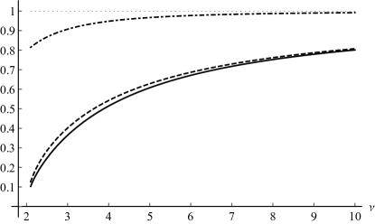
Figure B.2: Relative efficiency of $\hat{\beta}$ based on $q\geq 4$ vs. $q=2$ (solid line), $q=3$ vs. $q=2$ (dashed line), and $q\geq 4$ vs. $q=3$ (dash-dotted line) moment conditions as a function of $\nu$.

If $q\geq 4$, only the moment indicators $x^{j-1}u(z,\beta)$, $j=3,4$, are used to estimate $\beta_{0}$. Information in the remaining moment conditions, however, can be usefully exploited to improve the efficiency of the density estimators $\hat{f}$ and $\hat{f}_{\rho}$. The quantities entering the integrated variance eqs. (3.11) and (3.12) can be computed as $\mathop{\mathrm{tr}}\left(\Sigma{\textstyle\int}[\mathrm{d}\{\operatorname{E}[\nabla u_{i}|u]f(u)\}/\mathrm{d}u][\mathrm{d}\{\operatorname{E}[\nabla u_{i}|u]f(u)\}/\mathrm{d}u]^{\top}\mathrm{d}u\right)$, $\mathop{\mathrm{tr}}\left(H\int\operatorname{E}[g_{i}|u]\right.\\ \left.\times[\mathrm{d}\{\operatorname{E}[\nabla u_{i}|u]f(u)\}/\mathrm{d}u]^{\top}f(u)\mathrm{d}u\right)$, and $\mathop{\mathrm{tr}}\left(P\int\operatorname{E}[g_{i}|u]\operatorname{E}[g_{i}|u]^{\top}f(u)^{2}\mathrm{d}u\right)$, where

$$\int\tfrac{\mathrm{d}\{\operatorname{E}[\nabla u_{i}|u]f(u)\}}{\mathrm{d}u}\left(\tfrac{\mathrm{d}\{\operatorname{E}[\nabla u_{i}|u]f(u)\}}{\mathrm{d}u}\right)^{\top}\mathrm{d}u=\tfrac{\Gamma((\nu+3)/2)}{\omega^{3}\pi^{1/2}\nu^{3/2}\Gamma(\nu/2)}\left[\begin{smallmatrix}\tfrac{\nu\Gamma(\nu+3/2)\Gamma((\nu+3)/2)}{\Gamma(\nu/2+1)\Gamma(\nu+3)}&\tfrac{\nu^{1/2}\Gamma(\nu+3)}{2^{1/2}\Gamma(\nu+7/2)}\\ \tfrac{\nu^{1/2}\Gamma(\nu+3)}{2^{1/2}\Gamma(\nu+7/2)}&\tfrac{\Gamma(\nu+5/2)\Gamma(\nu/2+2)}{2\Gamma(\nu+2)\Gamma((\nu+5)/2)}\end{smallmatrix}\right],$$

the $q\times 2$ matrix ${\textstyle\int}\operatorname{E}[g_{i}|u][\mathrm{d}\{\operatorname{E}[\nabla u_{i}|u]f(u)\}/\mathrm{d}u]^{\top}f(u)\mathrm{d}u$ has rows

$$\tfrac{1}{(2\pi)^{1/2}\omega}\left[\tfrac{(2/\nu)^{i/2}\Gamma((\nu+3)/2)\Gamma(\nu+i/2)\Gamma((\nu+i)/2))}{\Gamma(\nu/2)^{2}\Gamma(\nu+(i+3)/2)},\quad\tfrac{(2/\nu)^{(i-1)/2}(\nu+2)\Gamma((\nu+1)/2)\Gamma(\nu+(i+1)/2)}{2\Gamma(\nu/2)\Gamma(\nu+i/2+2)}\right],\quad i=1,\ldots,q,$$

and the $q\times q$ matrix $\int\operatorname{E}[g_{i}|u]\operatorname{E}[g_{i}|u]^{\top}f(u)^{2}\mathrm{d}u$ with $(i,j)$th element

$$\omega m_{i}m_{j}\tfrac{\nu^{3/2}\Gamma(\nu+(i+j-3)/2)}{4\pi^{1/2}\Gamma(\nu+(i+j)/2)},\quad i,j=1,\ldots,q.$$

Remark B.2.

Figure B.3 shows the values of the above quantities and the overall effect on the integrated variance for selected values of $q$ and $\nu>2$; note that the validity of asymptotic expansions requires $\nu>4$, but variance is defined for $\nu>2$. While the main reduction in variance is still due to the zero mean restriction as in Example B.3 (Panels A and B), there are small additional gains due to re-weighting (Panel C). The latter do increase as more moment conditions are added.

(A) $\omega{\textstyle\int}[\mathrm{d}\{\operatorname{E}[\nabla u_{i}|u]f(u)\}/\mathrm{d}u]^{\top}\Sigma[\mathrm{d}\{\operatorname{E}[\nabla u_{i}|u]f(u)\}/\mathrm{d}u]\mathrm{d}u$	(A: zoom)
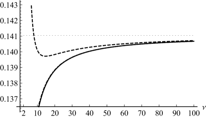
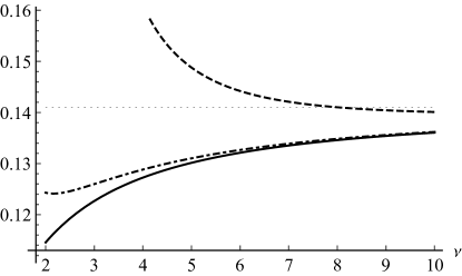
(B) $\omega{\textstyle\int}[\mathrm{d}\{\operatorname{E}[\nabla u_{i}|u]f(u)\}/\mathrm{d}u]^{\top}H\operatorname{E}[g_{i}|u]f(u)\mathrm{d}u$	(B: zoom)
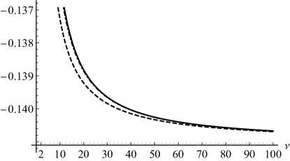
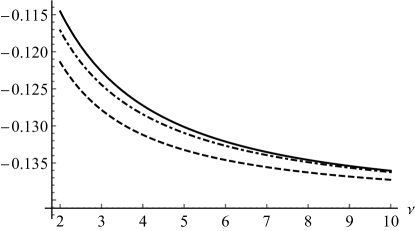
Legend to panels A and B: dashed line: $q=2$; dash-dotted line: $q=3$; solid line: $q\geq 4$.
(C) $\omega\int\operatorname{E}[g_{i}|u]^{\top}P\operatorname{E}[g_{i}|u]f(u)^{2}\mathrm{d}u$	(D) Overall effect: $(A)+2(B)-(C)$

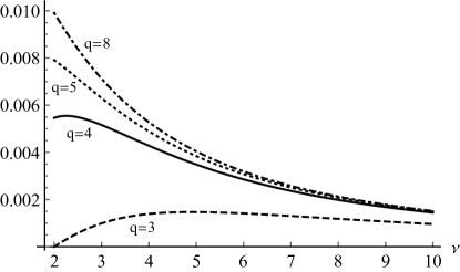
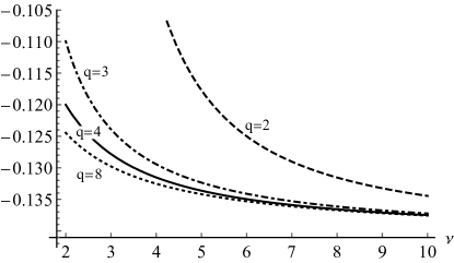
Figure B.3: Quantities entering the integrated variance of $\hat{f}$ and $\hat{f}_{\rho}$ in Example B.4 ($\times n\omega$)

References

- (1)
- Ahmad (1992) Ahmad, I. A. (1992), ‘Residuals density estimation in nonparametric regression’, Statistics & Probability Letters 14(2), 133–139. doi: 10.1016/0167-7152(92)90077-I
- Antoine et al. (2007) Antoine, B., Bonnal, H. and Renault, E. (2007), ‘On the efficient use of the informational content of estimating equations: Implied probabilities and Euclidean empirical likelihood’, Journal of Econometrics 138(2), 461–487. doi: 10.1016/j.jeconom.2006.05.005
- Back and Brown (1993) Back, K. and Brown, D. P. (1993), ‘Implied probabilities in GMM estimators’, Econometrica 61(4), 971–975. doi: 10.2307/2951771
- Bartlett (1963) Bartlett, M. S. (1963), ‘Statistical estimation of density functions’, Sankhyā: The Indian Journal of Statistics, Series A 25(3), 245–254. URL: www.jstor.org/stable/25049271
- Bhattacharya and Ghosh (1978) Bhattacharya, R. N. and Ghosh, J. K. (1978), ‘On the validity of the formal Edgeworth expansion’, The Annals of Statistics 6(2), 434–451. doi: 10.1214/aos/1176344134
- Bickel and Rosenblatt (1973) Bickel, P. J. and Rosenblatt, M. (1973), ‘On some global measures of the deviations of density function estimates’, The Annals of Statistics 1(6), 1071–1095. doi: 10.1214/aos/1176342558
- Bochner (1955) Bochner, S. (1955), Harmonic analysis and the theory of probability, University of California Press.
- Bott et al. (2013) Bott, A.-K., Devroye, L. and Kohler, M. (2013), ‘Estimation of a distribution from data with small measurement errors’, Electronic Journal of Statistics 7, 2457–2476. doi: 10.1214/13-EJS850
- Brown and Newey (1998) Brown, B. W. and Newey, W. K. (1998), ‘Efficient semiparametric estimation of expectations’, Econometrica 66(2), 453–464. doi: 10.2307/2998566
- Brown and Newey (2002) Brown, B. W. and Newey, W. K. (2002), ‘Generalized method of moments, efficient bootstrapping, and improved inference’, Journal of Business & Economic Statistics 20(4), 507–517. doi: 10.1198/073500102288618649
- Brown et al. (2015) Brown, S., Greene, W. H., Harris, M. N. and Taylor, K. (2015), ‘An inverse hyperbolic sine heteroskedastic latent class panel tobit model: An application to modelling charitable donations’, Economic Modelling 50, 228–236. doi: 10.1016/j.econmod.2015.06.018
- Burbidge et al. (1988) Burbidge, J. B., Magee, L. and Robb, A. L. (1988), ‘Alternative transformations to handle extreme values of the dependent variable’, Journal of the American Statistical Association 83(401), 123–127. doi: 10.1080/01621459.1988.10478575
- Cao and Lugosi (2005) Cao, R. and Lugosi, G. (2005), ‘Goodness-of-fit tests based on the kernel density estimator’, Scandinavian Journal of Statistics 32(4), 599–616. doi: 10.1111/j.1467-9469.2005.00471.x
- Chamberlain (1987) Chamberlain, G. (1987), ‘Asymptotic efficiency in estimation with conditional moment restrictions’, Journal of Econometrics 34(3), 305–334. doi: 10.1016/0304-4076(87)90015-7
- Chen and Qin (1993) Chen, J. and Qin, J. (1993), ‘Empirical likelihood estimation for finite populations and the effective usage of auxiliary information’, Biometrika 80(1), 107–116. doi: 10.1093/biomet/80.1.107
- Chen (1997) Chen, S. X. (1997), ‘Empirical likelihood-based kernel density estimation’, Australian and New Zealand Journal of Statistics 39(1), 47–56. doi: 10.1111/j.1467-842X.1997.tb00522.x
- Chen and Cui (2007) Chen, S. X. and Cui, H. (2007), ‘On the second-order properties of empirical likelihood with moment restrictions’, Journal of Econometrics 141(2), 492–516. doi: 10.1016/j.jeconom.2006.10.006
- Cheng (2004) Cheng, F. (2004), ‘Weak and strong uniform consistency of a kernel error density estimator in nonparametric regression’, Journal of Statistical Planning and Inference 119(1), 95–107. doi: 10.1016/S0378-3758(02)00417-2
- Cheng (2005) Cheng, F. (2005), ‘Asymptotic distributions of error density estimators in first-order autoregressive models’, Sankhyā: The Indian Journal of Statistics 67(3), 553–567. URL: http://www.jstor.org/stable/25053449
- Chernozhukov et al. (2009) Chernozhukov, V., Fernández-Val, I. and Galichon, A. (2009), ‘Improving point and interval estimators of monotone functions by rearrangement’, Biometrika 96(3), 559–575. doi: 10.1093/biomet/asp030
- Corcoran (1998) Corcoran, S. A. (1998), ‘Bartlett adjustment of empirical discrepancy statistics’, Biometrika 85(4), 967–972. doi: 10.1093/biomet/85.4.967
- Cox and Snell (1968) Cox, D. R. and Snell, E. J. (1968), ‘A general definition of residuals’, Journal of the Royal Statistical Society. Series B 30(2), 248–275. URL: www.jstor.org/stable/2984505
- Cressie and Read (1984) Cressie, N. and Read, T. R. C. (1984), ‘Multinomial goodness-of-fit tests’, Journal of the Royal Statistical Society. Series B 46(3), 440–464. URL: http://www.jstor.org/stable/2345686
- Fan (1994) Fan, Y. (1994), ‘Testing the goodness of fit of a parametric density function by kernel method’, Econometric Theory 10(2), 316–356. doi: 10.1017/S0266466600008434
- Fan (1998) Fan, Y. (1998), ‘Goodness-of-fit tests based on kernel density estimators with fixed smoothing parameters’, Econometric Theory 14(5), 604–621. doi: 10.1017/s0266466698145036
- Glad et al. (2003) Glad, I. K., Hjort, N. L. and Ushakov, N. G. (2003), ‘Correction of density estimators that are not densities’, Scandinavian Journal of Statistics 30(2), 415–427. doi: 10.1111/1467-9469.00339
- Györfi and Walk (2012) Györfi, L. and Walk, H. (2012), ‘Strongly consistent density estimation of the regression residual’, Statistics & Probability Letters 82(11), 1923–1929. doi: 10.1016/j.spl.2012.06.021
- Hall (2005) Hall, A. R. (2005), Generalized method of moments, Oxford University Press.
- Hansen et al. (1996) Hansen, L. P., Heaton, J. and Yaron, A. (1996), ‘Finite-sample properties of some alternative GMM estimators’, Journal of Business & Economic Statistics 14(3), 262–280. doi: 10.2307/1392442
- Imbens et al. (1998) Imbens, G. W., Spady, R. H. and Johnson, P. (1998), ‘Information theoretic approaches to inference in moment condition models’, Econometrica 66(2), 333–357. doi: 10.2307/2998561
- Jensen (1989) Jensen, J. L. (1989), ‘Validity of the formal Edgeworth expansion when the underlying distribution is partly discrete’, Probability Theory and Related Fields 81(4), 507–519. doi: 10.1007/BF00367300
- Johnson (1949) Johnson, N. L. (1949), ‘Systems of frequency curves generated by methods of translation’, Biometrika 36(1–2), 149–176. doi: 10.1093/biomet/36.1-2.149
- Kitamura and Stutzer (1997) Kitamura, Y. and Stutzer, M. (1997), ‘An information-theoretic alternative to generalized method of moments estimation’, Econometrica 65(4), 861–874. doi: 10.2307/2171942
- Kiwitt et al. (2008) Kiwitt, S., Nagel, E. and Neumeyer, N. (2008), ‘Empirical likelihood estimators for the error distribution in nonparametric regression models’, Mathematical Methods of Statistics 17(3), 241–260. doi: 10.3103/S1066530708030058
- Kundhi and Rilstone (2012) Kundhi, G. and Rilstone, P. (2012), ‘Edgeworth expansions for GEL estimators’, Journal of Multivariate Analysis 106, 118–146. doi: 10.1016/j.jmva.2011.11.005
- Loynes (1969) Loynes, R. M. (1969), ‘On Cox and Snell’s general definition of residuals’, Journal of the Royal Statistical Society. Series B 31(1), 103–106. URL: www.jstor.org/stable/2984331
- MacKinnon and Magee (1990) MacKinnon, J. G. and Magee, L. (1990), ‘Transforming the dependent variable in regression models’, International Economic Review 31(2), 315–339. doi: 10.2307/2526842
- Marron and Wand (1992) Marron, J. S. and Wand, M. P. (1992), ‘Exact mean integrated squared error’, The Annals of Statistics 20(2), 712–736. doi: 10.1214/aos/1176348653
- Mátyás (1999) Mátyás, L., ed. (1999), Generalized method of moments estimation, Cambridge University Press.
- Muhsal and Neumeyer (2010) Muhsal, B. and Neumeyer, N. (2010), ‘A note on residual-based empirical likelihood kernel density estimation’, Electronic Journal of Statistics 4, 1386–1401. doi: 10.1214/10-EJS586
- Nadaraya (1964) Nadaraya, E. A. (1964), ‘Some new estimates for distribution functions’, Theory of Probability and its Applications 9(3), 497–500. doi: 10.1137/1109069
- Newey and Smith (2004) Newey, W. K. and Smith, R. J. (2004), ‘Higher order properties of GMM and generalized empirical likelihood estimators’, Econometrica 72(1), 219–255. doi: 10.1111/j.1468-0262.2004.00482.x
- Oryshchenko (2017) Oryshchenko, V. (2017), Exact mean integrated squared error and bandwidth selection for kernel distribution function estimators, Working paper, University of Manchester. URL: https://arxiv.org/abs/1606.06993
- Owen (1988) Owen, A. (1988), ‘Empirical likelihood ratio confidence intervals for a single functional’, Biometrika 75(2), 237–249. doi: 10.1093/biomet/75.2.237
- Owen (1990) Owen, A. (1990), ‘Empirical likelihood ratio confidence regions’, The Annals of Statistics 18(1), 90–120. doi: 10.1214/aos/1176347494
- Pagan and Ullah (1999) Pagan, A. and Ullah, A. (1999), Nonparametric econometrics, Cambridge University Press.
- Parente and Smith (2014) Parente, P. M. and Smith, R. J. (2014), ‘Recent developments in empirical likelihood and related methods’, Annual Review of Economics 6, 77–102. doi: 10.1146/annurev-economics-080511-110925
- Parzen (1962) Parzen, E. (1962), ‘On estimation of a probability density function and mode’, The Annals of Mathematical Statistics 33(3), 1065–1076. doi: 10.1214/aoms/1177704472
- Qin and Lawless (1994) Qin, J. and Lawless, J. (1994), ‘Empirical likelihood and general estimating equations’, The Annals of Statistics 22(1), 300–325. doi: 10.1214/aos/1176325370
- Ramirez et al. (1994) Ramirez, O. A., Moss, C. B. and Boggess, W. G. (1994), ‘Estimation and use of the inverse hyperbolic sine transformation to model non-normal correlated random variables’, Journal of Applied Statistics 21(4), 289–304. doi: 10.1080/757583872
- Rao (1983) Rao, B. L. S. P. (1983), Nonparametric functional estimation, Academic Press.
- Robinson (1991) Robinson, P. M. (1991), ‘Best nonlinear three-stage least squares estimation of certain econometric models’, Econometrica 59(3), 755–786. doi: 10.2307/2938227
- Rosenblatt (1956) Rosenblatt, M. (1956), ‘Remarks on some nonparametric estimates of a density function’, The Annals of Mathematical Statistics 27(3), 832–837. doi: 10.1214/aoms/1177728190
- Schennach (2007) Schennach, S. M. (2007), ‘Point estimation with exponentially tilted empirical likelihood’, The Annals of Statistics 35(2), 634–672. doi: 10.1214/009053606000001208
- Silverman (1986) Silverman, B. W. (1986), Density Estimation for Statistics and Data Analysis, Chapman & Hall.
- Smith (1997) Smith, R. J. (1997), ‘Alternative semi-parametric likelihood approaches to generalised method of moments estimation’, The Economic Journal 107(441), 503–519. doi: 10.1111/j.0013-0133.1997.174.x
- Smith (2011) Smith, R. J. (2011), ‘GEL criteria for moment condition models’, Econometric Theory 27(6), 1192–1235. doi: 10.1017/S026646661100003X
- Stacy (1962) Stacy, E. W. (1962), ‘A generalization of the gamma distribution’, The Annals of Mathematical Statistics 33(3), 1187–1192. doi: 10.1214/aoms/1177704481
- Tsai et al. (2017) Tsai, A. C., Liou, M., Simak, M. and Cheng, P. E. (2017), ‘On hyperbolic transformations to normality’, Computational Statistics & Data Analysis 115, 250–266. doi: 10.1016/j.csda.2017.06.001
- Tsybakov (2009) Tsybakov, A. B. (2009), Introduction to Nonparametric Estimation, (Springer Series in Statistics), Springer. doi: 10.1007/b13794
- Van Ryzin (1969) Van Ryzin, J. (1969), ‘On strong consistency of density estimates’, The Annals of Mathematical Statistics 40(5), 1765–1772. doi: 10.1214/aoms/1177697388
- Wand and Jones (1995) Wand, M. P. and Jones, M. C. (1995), Kernel Smoothing, Chapman & Hall.
- Wand and Schucany (1990) Wand, M. P. and Schucany, W. R. (1990), ‘Gaussian-based kernels’, Canadian Journal of Statistics 18(3), 197–204. doi: 10.2307/3315450
- Watson and Leadbetter (1964) Watson, G. S. and Leadbetter, M. R. (1964), ‘Hazard analysis II’, Sankhyā: The Indian Journal of Statistics, Series A 26(1), 101–116. URL: http://www.jstor.org/stable/25049316
- Yamato (1973) Yamato, H. (1973), ‘Uniform convergence of an estimator of a distribution function’, Bulletin of Mathematical Statistics 15(3-4), 69–78. URL: http://ci.nii.ac.jp/naid/120001036895/
- Yuan et al. (2014) Yuan, A., Xu, J. and Zheng, G. (2014), ‘On empirical likelihood statistical functions’, Journal of Econometrics 178(3), 613–623. doi: 10.1016/j.jeconom.2013.08.037
- Zhang (1995) Zhang, B. (1995), ‘M-estimation and quantile estimation in the presence of auxiliary information’, Journal of Statistical Planning and Inference 44(1), 77–94. doi: 10.1016/0378-3758(94)00040-3
- Zhang (1998) Zhang, B. (1998), ‘A note on kernel density estimation with auxiliary information’, Communications in Statistics—Theory and Methods 27(1), 1–11. doi: 10.1080/03610929808832647
- Zygmund (2003) Zygmund, A. (2003), Trigonometric series, 3rd edn, Cambridge University Press.