Universality and quantum criticality of the one-dimensional spinor Bose gas

Abstract

We investigate the universal thermodynamics of the two-component one-dimensional Bose gas with contact interactions in the vicinity of the quantum critical point separating the vacuum and the ferromagnetic liquid regime. We find that the quantum critical region belongs to the universality class of the spin-degenerate impenetrable particle gas which, surprisingly, is very different from the single-component case and identify its boundaries with the peaks of the specific heat. In addition, we show that the compressibility Wilson ratio, which quantifies the relative strength of thermal and quantum fluctuations, serves as a good discriminator of the quantum regimes near the quantum critical point. Remarkably, in the Tonks-Girardeau regime the universal contact develops a pronounced minimum, reflected in a counterintuitive narrowing of the momentum distribution as we increase the temperature. This momentum reconstruction, also present at low and intermediate momenta, signals the transition from the ferromagnetic to the spin-incoherent Luttinger liquid phase and can be detected in current experiments with ultracold atomic gases in optical lattices.

Experiments with ultracold atomic gases allow for the creation and manipulation of various physical systems with an unprecedented degree of control over interaction strength, statistics of the constituent particles and dimensionality BDZ . This control materialized in the experimental realization of many low-dimensional systems whose physics is well captured by many-body integrable models allowing for a parameter free comparison between theory and experiment CCGOR ; GBL . The need for accurate theoretical predictions is particularly stringent in low-dimensions due to the enhancement of quantum fluctuations which invalidates our physical intuition based on the free-particle picture and mean-field theory. In the case of integrable models powerful techniques associated with Bethe Ansatz KBI ; EFGKK can be employed to analytically investigate the physical properties of such systems for all values of the interaction strength including the strong coupling limit.

One-dimensional (1D) multi-component systems in which the constituent particles have a variable number of internal “pseudospin” states present very rich physics exhibiting quantum regimes not found in higher dimensions or in the case of their single component counterparts CCGOR ; GBL ; WWD ; Pagano . As is well known, the single component Bose gas in the Tonks-Girardeau regime with infinitely strong coupling realizes an impenetrable particle gas which is fully described by spinless free fermions. We will see that the spinor gases in the very strong coupling regime behave very differently from free fermions.

At zero temperature these systems present Quantum Phase Transitions (QPT) which are driven by varying certain nonthermal parameters (chemical potential, magnetic field, pressure, etc.). In the vicinity of the Quantum Critical Point (QCP) quantum and thermal fluctuations couple strongly characterizing the Quantum Critical (QC) regime S . In the phase space the QC region has a distinct V-shape fanning out from the QCP S ; CS at low-temperatures and in this region the thermodynamics of the system is universal and scale invariant.

Motivated by the recent experimental confirmation Guan1 of quantum criticality in the Lieb-Liniger model LL in this Letter we theoretically investigate the more complex problem posed by the two-component generalization known as the spinor Bose gas Y1 ; G1 ; LGYE . We provide an analytical description of the universal thermodynamics and determine the location of the QCP, the critical exponents and the boundaries of the critical region. The analytical description is derived for arbitrary number of spin components. It is universally valid for bosons and fermions. It also explains the first order transition in the finite density regime with jump of the magnetization at zero magnetic field. In addition, for the two-component Bose case we perform a detailed analysis of the universal contact Tan1 ; OD ; BZ ; CJGZ and show that in the Tonks-Girardeau regime it presents a pronounced minimum signalling the transition from the ferromagnetic ZCG1 ; AT ; MF ; KG ; ZCG2 to the spin-incoherent liquid phase CZ1 ; FB ; F . This transition is accompanied by a significant momentum reconstruction which can be experimentally detected.

We consider a system of 1D bosons with two internal “pseudospin” states denoted by $\uparrow$ and $\downarrow$ with spin-independent contact interactions. In second quantization the Hamiltonian is $H=\int\mathcal{H}(x)\,dx$ with density

$$\mathcal{H}(x) =\sum_{\sigma=\{\uparrow,\downarrow\}}\left(\frac{\hbar^{2}}{2m}\partial_{x}\Psi^{\dagger}_{\sigma}(x)\partial_{x}\Psi_{\sigma}(x)-\mu_{\sigma}\Psi^{\dagger}_{\sigma}(x)\Psi_{\sigma}(x)\right)\,$$

$$\ \ \ \ \ +\frac{\hbar^{2}c}{2m}\sum_{\sigma,\sigma^{\prime}=\{\uparrow,\downarrow\}}\Psi^{\dagger}_{\sigma}(x)\Psi^{\dagger}_{\sigma^{\prime}}(x)\Psi_{\sigma^{\prime}}(x)\Psi_{\sigma}(x)$$ (1)

where $\Psi_{\sigma}(x),\Psi_{\sigma}^{\dagger}(x)$ are bosonic fields satisfying $[\Psi_{\sigma}(x),\Psi^{\dagger}_{\sigma^{\prime}}(y)]=\delta_{\sigma,\sigma^{\prime}}\delta(x-y)$, $m$ is the mass of the particles, $\mu_{\sigma}$ are chemical potentials and the coupling constant can be expressed in terms of the 1D scattering length via $c=-2/a_{1D}$ Ol . In the following it will be useful to introduce $\mu=(\mu_{\uparrow}+\mu_{\downarrow})/2$ and $H=(\mu_{\uparrow}-\mu_{\downarrow})/2$. In units of $\hbar=2m=1$ the dimensionless coupling constant is $\gamma=c/n$ with $n$ the total density and the Fermi temperature is $T_{F}=\pi^{2}n^{2}$. The system is weakly (strongly) interacting when $\gamma\ll 1\,(\gamma\gg 1)$.

The Hamiltonian (Universality and quantum criticality of the one-dimensional spinor Bose gas) is integrable Y1 ; G1 and the ground state and low-lying excitations were derived using the Nested Bethe Ansatz LGYE . Compared with the fermionic model, for which the ground-state is antiferromagnetic, in this case the ground-state is fully polarized (ferromagnetic) which is a general characteristic of bosonic 1D models with spin-independent interactions EL . At low temperatures the longitudinal low-lying excitations are plasmons ($\epsilon(p)\sim|p|$) but the softest transversal low-lying excitation is a magnon with quadratic dispersion $\lim_{p\rightarrow 0}\epsilon(p)\sim p^{2}/2m_{*}\,$ which prevents the use of the Luttinger liquid (LL) theory ($m_{*}=3m\,\gamma/2\pi^{2}\,$ for large $\gamma$ FGKS ).

Computing the thermodynamic properties of the spinor Bose gas is a notoriously difficult task despite the integrability of the Hamiltonian (Universality and quantum criticality of the one-dimensional spinor Bose gas). In contrast with the single component case (the Lieb-Liniger model) the Thermodynamic Bethe Ansatz (TBA) YY ; T description of the multi-component model GLYZ involves an infinite number of nonlinear integral equations (NLIEs). Even though numerical schemes can be developed to approximately solve such systems CKB ; KC ; GBT they are rather cumbersome and require truncations in the number of equations which can introduce uncontrollable errors. In KP1 ; PK1 two of the authors derived an efficient thermodynamic description which made use of the lattice embedding of the spinor Bose gas in the $q=3$ Perk-Schultz spin chain and the Quantum Transfer Matrix EFGKK ; K1 ; K2 . In this description the grand-canonical potential per length is given by $\phi(\mu,H,T)=-\frac{T}{2\pi}\int_{-\infty}^{+\infty}\ln[1+a_{1}(k)]+\ln[1+a_{2}(k)]\,dk\,,$ with $a_{i}(k)$ auxiliary functions satisfying the following system of NLIEs:

$$\ln a_{1}(k) =-(k^{2}-\mu-H)/T$$

$$\ \ +[K_{0}*\ln A_{1}](k)+[K_{2}*\ln A_{2}](k-i\epsilon)\,,$$ (2a)

$$\ln a_{2}(k) =-(k^{2}-\mu+H)/T$$

$$\ \ +[K_{1}*\ln A_{1}](k+i\epsilon)+[K_{0}*\ln A_{2}](k)\,,$$ (2b)

where $A_{i}(k)=1+a_{i}(k)\,,$ $K_{0}(k)=2c/(k^{2}+c^{2})\,,$ $K_{1}(k)=c/[k(k+ic)]\,,K_{2}(k)=c/[k(k-ic)]$ and $[f*g](k)=\frac{1}{2\pi}\int_{-\infty}^{+\infty}f(k-k^{\prime})g(k^{\prime})\,dk^{\prime}.$ We stress that Eqs. (2) are valid for all values of $\mu\,,H\,,T$ and $c$ and they can be easily and efficiently numerically implemented allowing for the exploration of certain regions of the relevant parameters space (like $H\ll T,\mu,c$) which are inaccessible by TBA. These equations constitute the basis of our investigations.

At $T=0$ and fixed $H$ the spinor Bose gas presents a QPT between the vacuum and ferromagnetic liquid phase when the chemical potential reaches the QCP. In the vicinity of the QCP the thermodynamics of the system is universal and scale invariant and can be described by ZH ; FWGF

$$p(\mu,H,T)\sim p_{r}(\mu,H,T)+T^{\frac{d}{z}+1}\mathcal{P}_{H}\left(\frac{\mu-\mu_{c}(H)}{T^{\frac{1}{\nu z}}}\right)$$ (3)

where $p=-\phi$ is the pressure, $p_{r}$ the regular part, $z$ the dynamical critical exponent, $\nu$ the correlation length exponent, $d=1$ the dimension and $\mathcal{P}_{H}$ is a universal function describing the singular part of the pressure. The determination of the universality class (the values of $z$ and $\nu$) and of the universal function is accomplished by performing the following steps ZH : i) Choose $z$ and $\nu$ ii) For these values of $z$ and $\nu$ plot for several values of temperature the “scaled pressure” $(p-p_{r})T^{-\frac{d}{z}-1}$ (at low-$T$ $p_{r}$ can be replaced by a constant which in our case is zero). If the critical exponents are chosen correctly then all plots should intersect at $\mu_{c}(H)$ identifying the QCP. iii) With $z$, $\nu$ and $\mu_{c}(H)$ determined the plots of the “scaled pressures” at all temperatures as functions of $(\mu-\mu_{c}(H))/T^{\frac{1}{\nu z}}$ will collapse to a single curve which is the universal function $\mathcal{P}_{H}$.

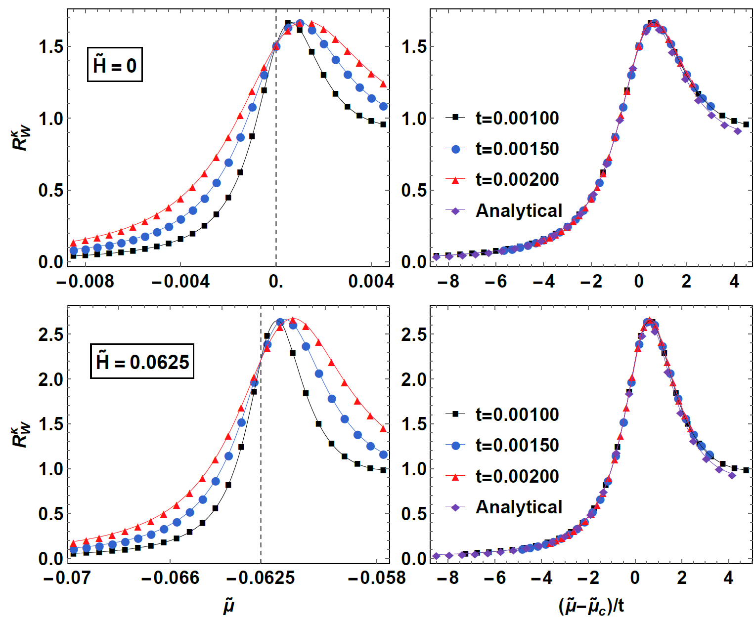
Figure 1: Scaling behaviour of the compressibility Wilson ratio $R_{W}^{\kappa}$ for $\tilde{H}=0$ (upper panels) and $\tilde{H}=0.0625$ (lower panels) ($\tilde{H}=H/c^{2},\tilde{\mu}=\mu/c^{2},t=T/c^{2}$ with $c=2$). The curves at different temperatures intersect at the QCP $\tilde{\mu}_{c}=-|\tilde{H}|$. Plots of the ratio as function of $(\tilde{\mu}-\tilde{\mu}_{c})/t$ reveal the universal function $\mathcal{Q}_{H}(x)$. In the right panels the magenta diamonds represent the analytical predictions given by Eq. (4) with $e^{-|y|}=0$ for $H\neq 0$ and $e^{-|y|}=1$ for $H=0$.

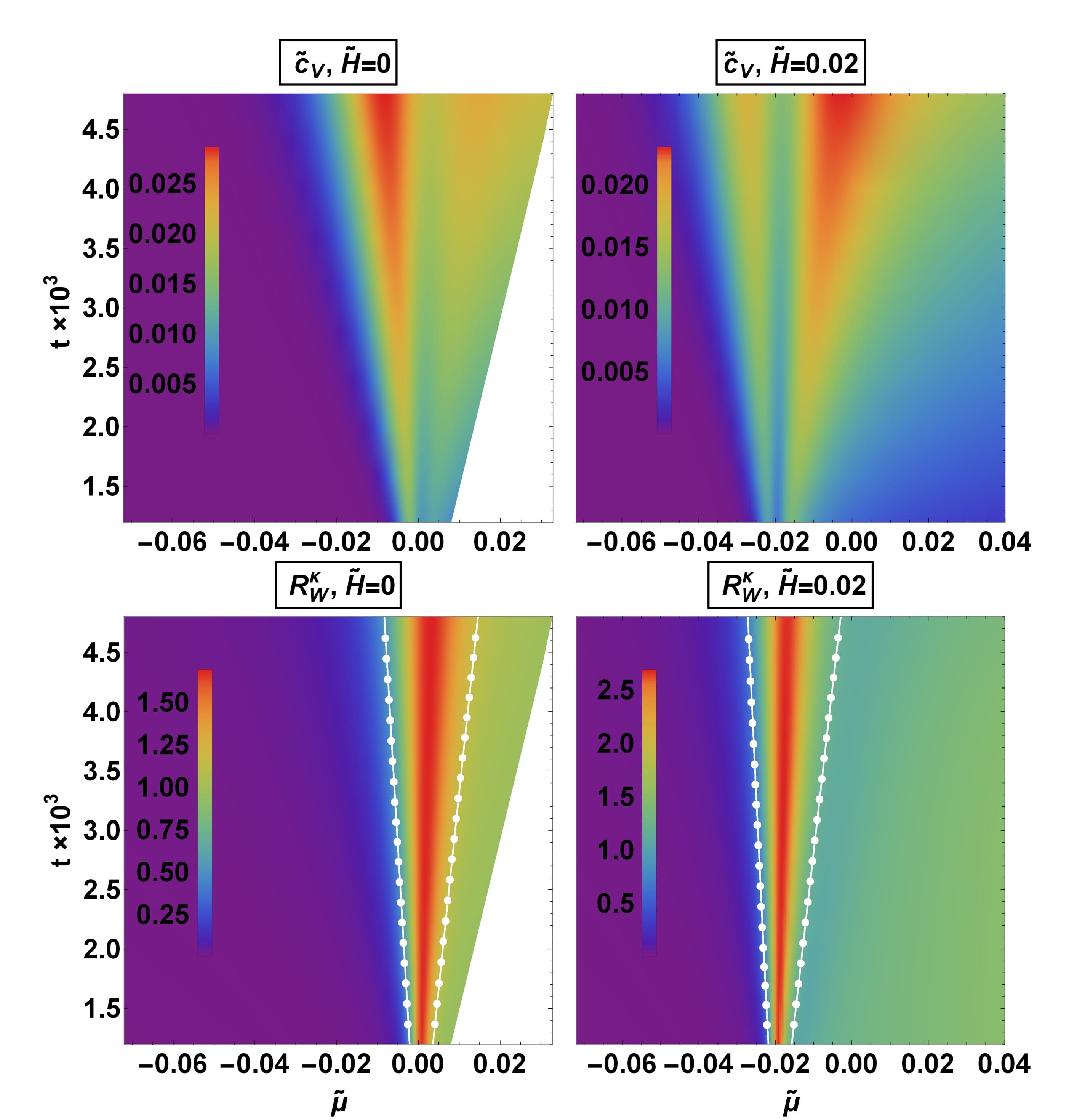
Figure 2: Density plots of the grand-canonical specific heat $\tilde{c}_{V}=c_{V}/c$ (upper panels) and Wilson ratio (lower panels) for $\tilde{H}=0$ and $\tilde{H}=0.02$ ($c=5$). The specific heat presents maxima fanning out from the critical value of chemical potential $\mu_{c}=-|H|$ which determine the boundaries of the QC region. The white lines in the Wilson ratio plots are the boundaries of the QC region given by the maxima of the specific heat. To the left of the boundary lies the vacuum phase at finite temperature which can be well approximated by a classical gas and to the right the ferromagnetic liquid regime.

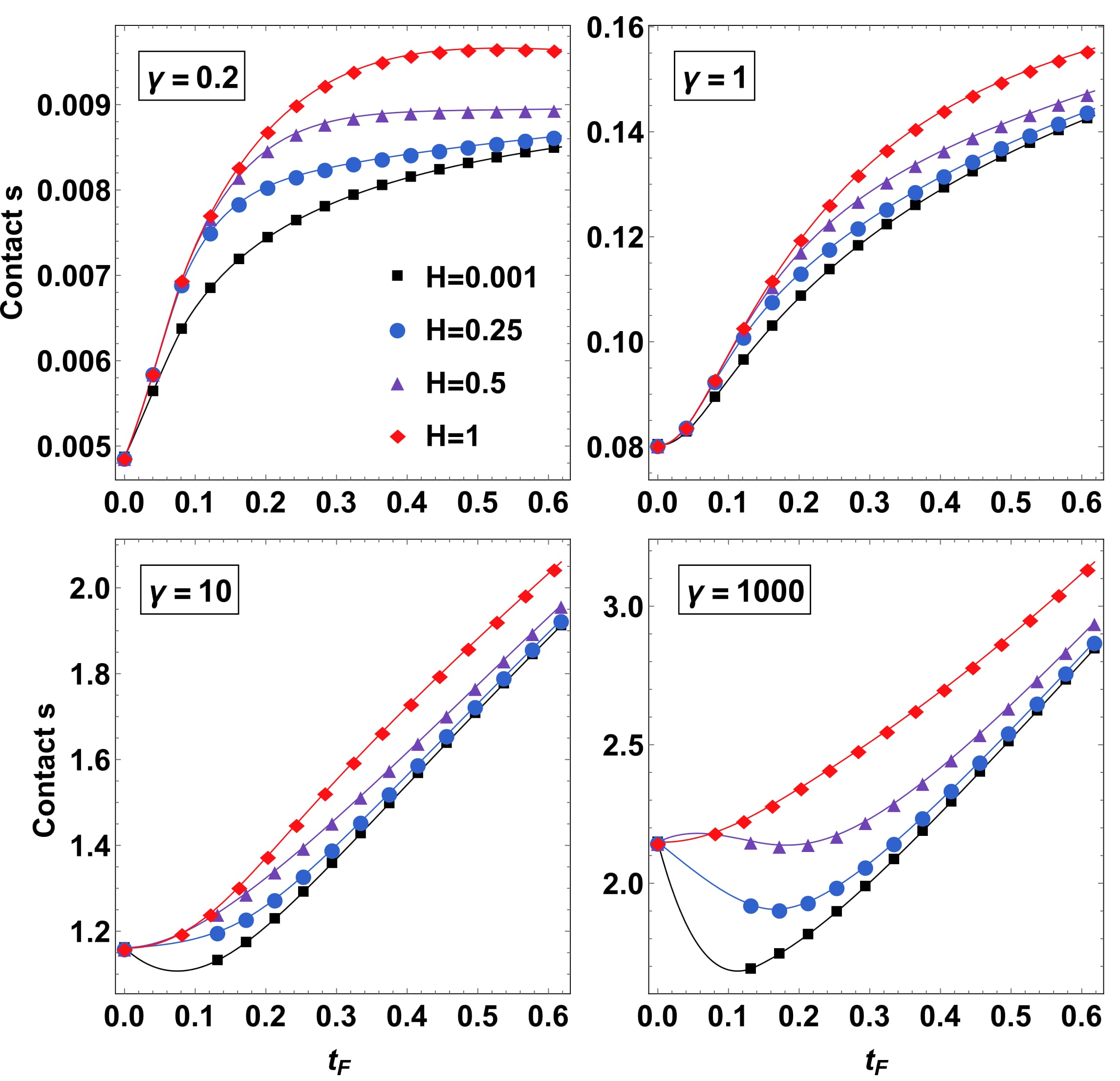
Figure 3: Dependence of the dimensionless total contact $s$ on the temperature ($t_{F}=T/T_{F}\,,\gamma=c/n\,,n=1/2$) for $\gamma=\{0.2,1,10,1000\}$ and several values of $H$. At strong coupling and low $H$ the contact develops a minimum.

Our investigations reveal SuplM lines of QCPs at $\mu_{c}(H)=-|H|$ with critical exponents $z=2$ and $\nu=1/2$. We identify the universality class as the spin-degenerate impenetrable particle gas. This can be understood intuitively by an elementary, yet quantitative derivation. For any repulsive interaction, at low densities the system is in the strong coupling regime with finite energy states realized by wave functions $\psi(x_{1},...,x_{N},s_{1},...,s_{N})$ that vanish if the spatial coordinates of any two particles coincide. We construct such wave functions by first considering the fundamental regime with order of spatial coordinates $x_{1}<x_{2}<\cdots<x_{N}$. Here, we use the product ansatz $\phi\cdot\chi$ where $\phi(x_{1},...,x_{N})$ is a Slater determinant of plane waves with pairwise different wave numbers $k_{1},...,k_{N}$ and $\chi=|\sigma_{1},...,\sigma_{N}\rangle$ is an arbitrary spin part. For all other sectors with different order of spatial coordinates we reorder simultaneously all spatial and spin coordinates leading to the fundamental regime and then invoking the symmetry of the total wave function.

The energy of the product states is given by the sum of the kinetic energy terms ($k^{2}$) and the Zeeman terms ($\pm H$). We set up the partition function of the grand-canonical ensemble. The space of configurations consists of all combinations of occupations of $k$-modes: empty, singly occupied with spin up or spin down. The partition function is a product over characteristic factors $Z=\prod_{k}\left[1+e^{-\beta(k^{2}-\mu-H)}+e^{-\beta(k^{2}-\mu+H)}\right]$ for all $k$ values allowed by the boundary conditions. Note that this derivation with exactly the same result also works for fermions with infinitely strong repulsion. The generalization to arbitrary spin numbers is obvious.

The universal thermodynamics (for both fermions and bosons) in the vicinity of the QCP is given by Takahashi’s formula T ($x=(\mu+|H|)/T\,,y=H/T$)

$$p=\frac{T^{3/2}}{2\pi}\int_{-\infty}^{+\infty}\ln\left[1+(1+e^{-2|y|})e^{-k^{2}+x}\right]\,dk\,.$$ (4)

Fig. 1 shows the collapse of Wilson ratio (see below) data onto the universal function analytically derived from Eq. (4). Also, the structures of the QC regime are fully described by Eq. (4), see Fig. 2. Despite its apparent simplicity, the spin degenerate impenetrable particle gas has a rich phase diagram and surprising properties. The critical exponents suggest that the system might be equivalent to free fermions with the pressure given by ($x^{\prime}=\mu/T$), $p_{FF}=\frac{T^{3/2}}{2\pi}\int\ln\left[\left(1+e^{-k^{2}+x^{\prime}+y}\right)\left(1+e^{-k^{2}+x^{\prime}-y}\right)\right]\,dk\,.$ However, free fermions have a $\mu-H$ phase diagram with four phases (vacuum, spin-up particles, spin-down particles and the mixture of spin-up and spin-down particles) and critical lines $\mu=\pm H$. In contrast, the spin-degenerate impenetrable particle gas has only three phases (vacuum, spin-up particles and spin-down particles) with critical lines $\mu=-|H|$ and $\mu>0,H=0$. At the latter line, first order transitions take place. Here, simply by taking the H-derivative of Eq. (4) (see also SuplM ), we find a magnetization with jump at zero field $m\sim\hbox{sign}H\,(\mu+|H|)^{1/2}/\pi,$ and at $T=H=0$ also residual entropy $s\sim\mu^{1/2}\ln 2/\pi\,!$ Despite the deceiving familiar values of the critical exponents the physics of the spin-degenerate impenetrable particle gas is drastically different from that of ordinary free fermions.

It was shown in YCLRG ; GYFBLL ; Guan2 that the susceptibility and compressibility Wilson ratios can serve as good discriminators of quantum phases in attractive multi-component ultracold gases. In our case the relevant quantity is the compressibility Wilson ratio defined by $R_{W}^{\kappa}=\frac{\pi^{2}k_{B}^{2}}{3}T\frac{\kappa}{c_{V}}$ with $\kappa=-\partial^{2}\phi/\partial\mu^{2}$ the compressibility $c_{V}=-T\partial^{2}\phi/\partial T^{2}$ the grand-canonical specific heat at constant volume. In the vicinity of the QCP the Wilson ratio scales like $R_{W}^{\kappa}\sim\mathcal{Q}_{H}\left(\frac{\mu-\mu_{c}(H)}{T}\right)$ with $\mathcal{Q}_{H}(x)=\mathcal{P}_{H}^{{}^{\prime\prime}}(x)/\left(\frac{3}{4}\mathcal{P}_{H}(x)-x\mathcal{P}^{\prime}_{H}(x)+x^{2}\mathcal{P}_{H}^{{}^{\prime\prime}}(x)\right)$ a universal function. In the vacuum phase $R_{W}^{\kappa}$ is zero and presents a sudden enhancement in the QC region becoming almost constant in the ferromagnetic liquid phase. Taking into account that in the grand-canonical ensemble the compressibility and specific heat quantify the energy and particle fluctuations via $k_{B}T\kappa=\langle\delta N^{2}\rangle$ and $k_{B}T^{2}c_{V}=\langle\delta(E-\mu N)^{2}\rangle$ it is easy to understand why $R_{W}^{\kappa}$ identifies the quantum regimes so efficiently. In the critical regime the thermal and quantum fluctuations couple strongly resulting in the anomalous enhancement in the vicinity of the QCP. In the upper panels of Fig. 2 we show that the specific heat presents a continuous set of local maxima on both sides of the QCP, peaks that can be identified with the boundaries of the QC region (see also Guan1 ; Guan2 ; MHO ). Depicting these boundaries in the density plots of the Wilson ratio (lower panels of Fig. 2) we see that they clearly delimitate the three quantum regimes.

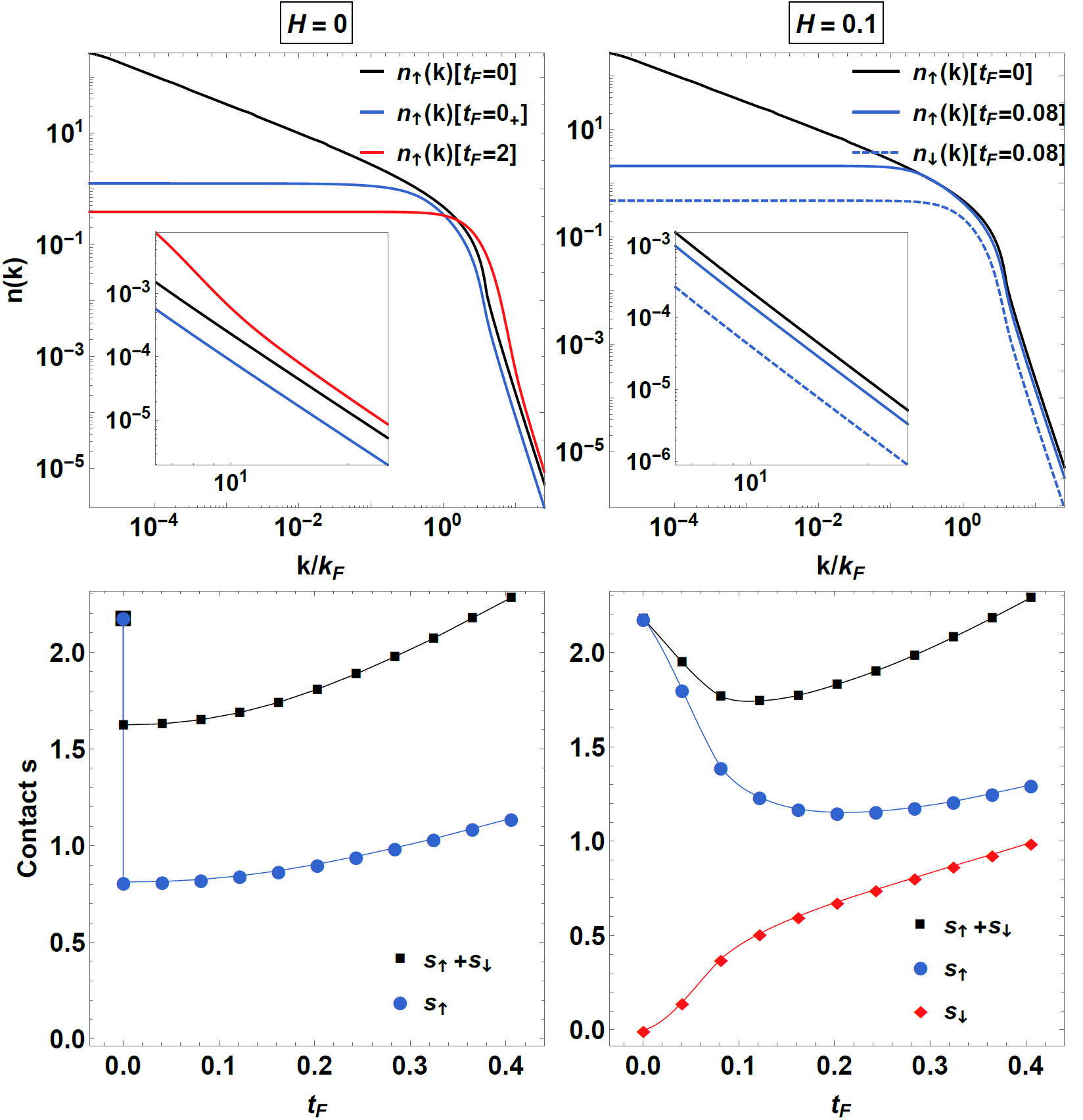
Figure 4: Upper left panel: Momentum distribution in log-log coordinates for the balanced impenetrable gas ($H=0$) for $t_{F}=\{0,0_{+},2\}$. For the balanced system at a fixed temperature $n_{\uparrow}(k)=n_{\downarrow}(k)$. Data show a significant momentum reconstruction especially at low and high momenta as we increase the temperature from the ferromagnetic liquid $(t_{F}=0)$ to the spin-incoherent LL regime $(t_{F}=0_{+})$. The inset shows the high momentum tail from which the contact can be extracted and shows that $s_{\uparrow}(t_{F}=0)>s_{\uparrow}(t_{F}=0_{+}).$ Lower left panel: Dependence of the dimensionless total contact $s_{\uparrow}+s_{\downarrow}$ (black squares) and contact of spin-up particles $s_{\uparrow}$ (blue disks) as functions of the temperature for the balanced system. While at $t_{F}=0$ the ground state is populated only by type 1 particles, at $t_{F}=0_{+}$ the system is balanced and $s_{\uparrow}=s_{\downarrow}$. The total contact and also $s_{\uparrow}$ present a sharp minimum at $t_{F}=0_{+}$. Upper right panel: Momentum distribution for $H=0.1$ and $t_{F}=\{0,0.08\}$. In this case for a fixed temperature $n_{\uparrow}(k)\neq n_{\downarrow}(k)$. Data also show a significant momentum reconstruction but not as pronounced as in the balanced case. The inset shows that $s_{\uparrow}(t_{F}=0)>s_{\uparrow}(t_{F}=0.08)>s_{\downarrow}(t_{F}=0.08)$. Lower right panel: Temperature dependence of the contact for $H=0.1$. Even though $s_{\downarrow}$ is monotonously increasing, the total contact and $s_{\uparrow}$ present a local minimum at low temperatures. In all cases $n=1/2$.

A universal property of physical systems with contact interactions is that the large momentum distribution behaves like $\lim_{k\rightarrow\infty}n_{\sigma}\sim\mathcal{C}_{\sigma}/k^{4}$ with $\mathcal{C}_{\sigma}$ the amplitude called contact Tan1 ; OD ; BZ ; CJGZ ; PK2 . In the case of the bosonic Gaudin-Yang model the total contact can be computed from the thermodynamics PK2 as $\mathcal{C}=\mathcal{C}_{\uparrow}+\mathcal{C}_{\downarrow}=c^{2}\partial^{2}\phi/\partial c^{2}.$ In Fig. 3 we show the temperature dependence of the dimensionless total contact $s=\mathcal{C}/k_{F}^{4}$ with $k_{F}=\pi n$ for several values of coupling constant and magnetic field. For $\gamma=\{0.2,1\}$ it is a monotonously increasing function of the temperature for all values of $H$. At strong coupling the contact develops a minimum at low temperatures which is more pronounced as $H$ decreases. This means that for $\gamma\gg 1$ we encounter the counterintuitive phenomenon in which the fraction of particles with high momenta decreases as we increase the temperature. It was first noticed in CSZ for the case of impenetrable particles at $H=0$ that this momentum reconstruction signals the transition from the ferromagnetic liquid phase $(T<T_{0}\sim T_{F}/\gamma)$ to the spin-incoherent LL regime $(T_{0}<T<T_{F})$ CZ1 ; FB ; F . The two temperature scales become well separated for $\gamma\gg 1$ which explains why we encounter this phenomenon only in the strong coupling limit.

In the impenetrable case the momentum distribution and the contact of each species of particles can be computed using the Fredholm determinant representation for the Green’s function $\langle\Psi_{i}^{\dagger}(x)\Psi_{i}(0)\rangle_{T,\mu,H}$ obtained in IP1 . Its Fourier transform yields the momentum distribution $n_{i}(k)$ and the contact is extracted as $C_{i}=\lim_{k\rightarrow\infty}n_{i}(k)/k^{4}.$ The detailed results in Fig. 4 reveal in addition to the high momentum crossover also a significant momentum reconstruction at low-momenta. This reconstruction, which takes place in a very narrow interval of temperature, is largest for the balanced system (see the left panels of Fig. 4) and becomes more attenuated as we increase $H$. The low-momentum crossover has a simple explanation. At $T=H=0$ the system is described by the impenetrable Lieb-Liniger model for which the groundstate is a quasicondensate with $n_{\uparrow}(k)\sim 1/\sqrt{k}$ for small k (corresponding to the large distance asymptotics of the Green’s function $\sim 1/x^{1/2}$). As we increase the temperature the system is described by the spin-incoherent LL with exponentially decreasing Green’s function at large distances CSZ and a finite momentum distribution at low-momenta. The same type of reasoning also holds for strong but finite coupling implying that the momentum reconstruction both at low- and high-momenta can be experimentally observed even for moderate values of $\gamma$.

In summary, we have investigated the universal properties of the spinor Bose gas and identified the universality class and boundaries of the QC region separating the vacuum from the ferromagnetic liquid phase. The universal contact increases with increasing magnetic field opposite to the behaviour of fermionic systems. In the Tonks-Girardeau regime the contact develops a pronounced minimum indicating a significant momentum reconstruction at low-temperatures which can be detected in current experiments with ultra-cold gases.

Supplemental Material: Universality and quantum criticality of the one-dimensional spinor Bose gas

I Scaling behaviour in the vicinity of the Quantum Critical Point

We can derive the scaling behaviour of the thermodynamic quantities in the vicinity of the QCP from the knowledge of the regular part of the pressure $p_{r}(\mu,H,T)$ and the universal function $\mathcal{P}_{H}$. In the case of the density and compressibility starting from Eq. (3), introducing the variable $x=(\mu-\mu_{c}(H))/T^{\frac{1}{\nu z}}$ and using $\phi(\mu,H,T)=-p(\mu,H,T)\,,$ $n=-\partial\phi/\partial\mu$ and $\kappa=-\partial^{2}\phi/\partial\mu^{2}$ we find

$$n(\mu,H,T)\sim\frac{\partial p_{r}(\mu,H,T)}{\partial\mu}+T^{\frac{d}{z}+1-\frac{1}{\nu z}}\mathcal{P}^{\prime}_{H}\left(x\right)\,,\ \ \ \ \kappa(\mu,H,T)\sim\frac{\partial^{2}p_{r}(\mu,H,T)}{\partial\mu^{2}}+T^{\frac{d}{z}+1-\frac{2}{\nu z}}\mathcal{P}_{H}^{{}^{\prime\prime}}\left(x\right)\,,$$ (S1)

where $\mathcal{P}^{\prime}_{H}(x)$ and $\mathcal{P}_{H}^{{}^{\prime\prime}}(x)$ are the first and second derivative of $\mathcal{P}_{H}(x)$. The scaling of the pressure and density ($\tilde{p}_{r}=\tilde{n}_{r}\sim 0$) which shows that the critical exponents are $z=2$ and $\nu=1/2$ is presented in Figs. S1 and S2. In a similar fashion we can obtain the scaling behaviour for the entropy $s=-\partial\phi/\partial T$ and grand-canonical specific heat $c_{V}=-T\partial^{2}\phi/\partial T^{2}$

$$s(\mu,H,T) \sim\frac{\partial p_{r}(\mu,H,T)}{\partial T}+T^{\frac{d}{z}}\left[\left(\frac{d}{z}+1\right)\mathcal{P}_{H}(x)-\frac{1}{\nu z}\,x\,\mathcal{P}^{\prime}_{H}(x)\right]\,,$$ (S2)

$$c_{V}(\mu,H,T) \sim\frac{\partial^{2}p_{r}(\mu,H,T)}{\partial T^{2}}+T^{\frac{d}{z}-1}\left\{\frac{d}{z}\left(\frac{d}{z}+1\right)\mathcal{P}_{H}(x)-\left[\frac{1}{\nu z}\left(\frac{2d}{z}+1\right)-\frac{1}{(\nu z)^{2}}\right]\,x\,\mathcal{P}^{\prime}_{H}(x)+\frac{1}{(\nu z)^{2}}\,x^{2}\,\mathcal{P}^{{}^{\prime\prime}}_{H}(x)\right\}\,.$$ (S3)

From Eqs. S1 and S3 and taking into account that for the QPT from the vacuum to the ferromagnetic liquid phase $p_{r}(\mu,H,T)\sim 0$ we obtain the scaling behaviour of the compressibility Wilson ratio $R_{W}^{\kappa}=\frac{\pi^{2}k_{B}^{2}}{3}T\frac{\kappa}{c_{V}}\sim\frac{\pi^{2}k_{B}^{2}}{3}\mathcal{Q}_{H}(x)$ with $\mathcal{Q}_{H}(x)=\mathcal{P}_{H}^{{}^{\prime\prime}}(x)/\left(\frac{3}{4}\mathcal{P}_{H}(x)-x\mathcal{P}^{\prime}_{H}(x)+x^{2}\mathcal{P}_{H}^{{}^{\prime\prime}}(x)\right).$

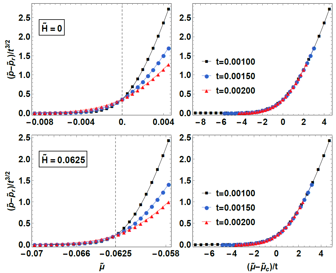
Figure S1: Scaling behaviour of the pressure $\tilde{p}=p/c^{3}$ for $\tilde{H}=0$ (upper panels) and $\tilde{H}=0.0625$ (lower panels) ($\tilde{H}=H/c^{2},\tilde{\mu}=\mu/c^{2},t=T/c^{2}$ with $c=2$). The curves at different temperatures intersect at the QCP $\tilde{\mu}_{c}=-|\tilde{H}|$. Plots of the pressure as function of $(\tilde{\mu}-\tilde{\mu}_{c})/t$ reveal the universal function $\mathcal{P}_{H}(x)$.

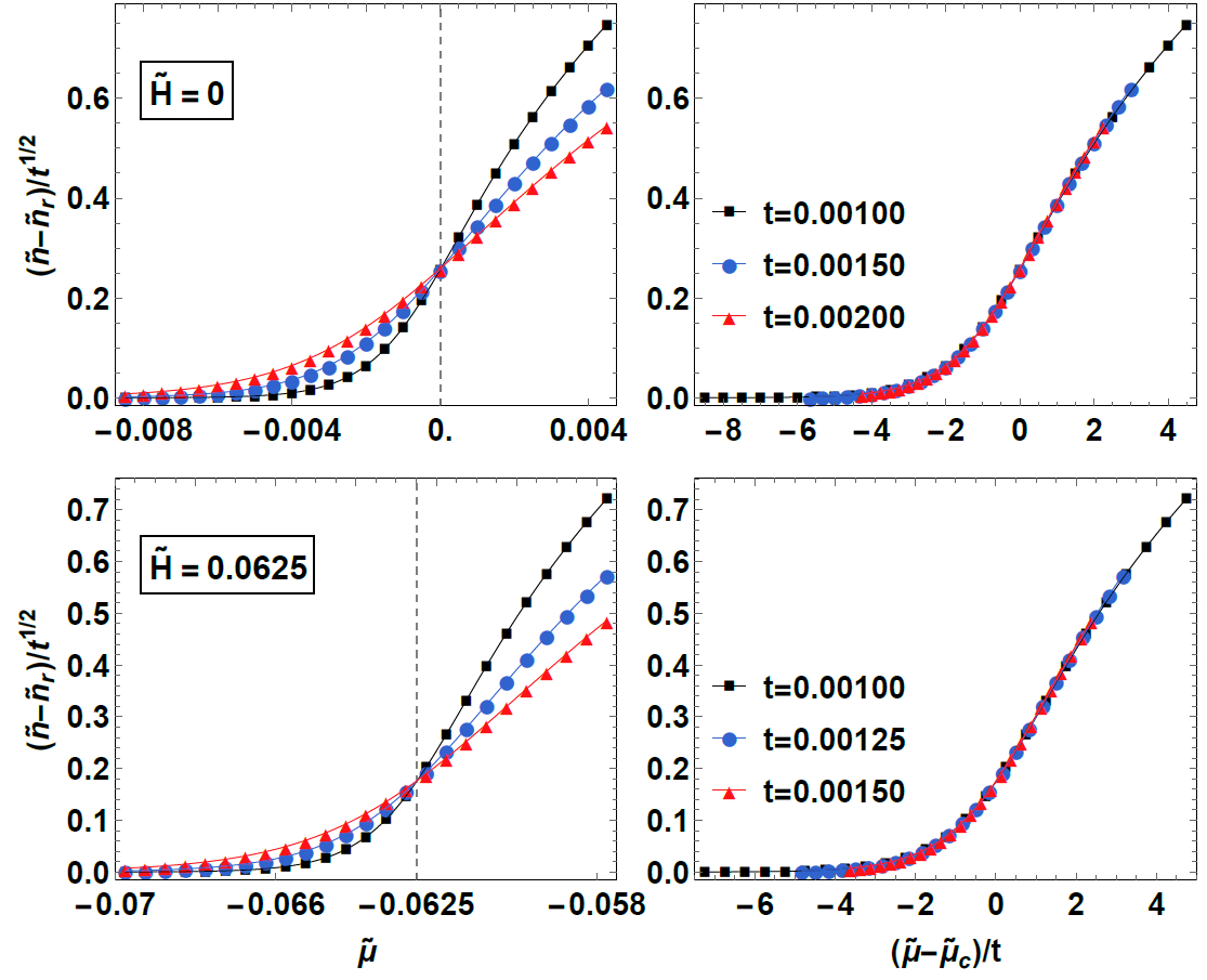
Figure S2: Scaling behaviour of the density $\tilde{n}=n/c$ for $\tilde{H}=0$ (upper panels) and $\tilde{H}=0.0625$ (lower panels) ($\tilde{H}=H/c^{2},\tilde{\mu}=\mu/c^{2},t=T/c^{2}$ with $c=2$). The curves at different temperatures intersect at the QCP $\tilde{\mu}_{c}=-|\tilde{H}|$. Plots of the density as function of $(\tilde{\mu}-\tilde{\mu}_{c})/t$ reveal the universal function $\mathcal{P}^{\prime}_{H}(x)$.

II Asymptotic analysis of the scaling function

Here we investigate the asymptotic properties of Takahashi’s formula

$$p=T^{3/2}\mathcal{P}_{y}(x)\,,\ \ \ \ \ \ \mathcal{P}_{y}(x)=\frac{1}{\pi}\int_{0}^{\infty}\ln\left[1+(1+e^{-2|y|})e^{-k^{2}+x}\right]\,dk\,,$$ (S4)

which describes the thermodynamics of 1D impenetrable two-component repulsive fermions and can be derived from the $c\rightarrow\infty$ limit of the TBA equations. While this formula was first obtained in the case of the impenetrable 2CFG it is also valid for the 2CBG and Bose-Fermi mixture in the same limit.

The large $x$ limit. We introduce the notation $\alpha=x+\ln\left(1+e^{-2|y|}\right)$ (large $x$ implies also large $\alpha$) and successively perform an integration by parts and changes of variables $k^{\prime}=k^{2}$ and $z=k^{\prime}-\alpha$ obtaining

$$\mathcal{P}_{y}(x)=\frac{1}{\pi}\int_{-\alpha}^{\infty}\frac{(z+\alpha)^{1/2}}{e^{z}+1}\,dz\,=\frac{1}{\pi}\int_{-\alpha}^{0}\frac{(z+\alpha)^{1/2}}{e^{z}+1}\,dz+\frac{1}{\pi}\int_{0}^{\infty}\frac{(z+\alpha)^{1/2}}{e^{z}+1}\,dz\,\,.$$

Switching to $z=-z$ in the first term on the r.h.s. of the previous identity and using $1/(e^{-z}+1)=1-1/(e^{z}+1)$ we find

$$\frac{1}{\pi}\int_{-\alpha}^{0}\frac{(z+\alpha)^{1/2}}{e^{z}+1}\,dz=\frac{1}{\pi}\int_{0}^{\alpha}\frac{(\alpha-z)^{1/2}}{e^{-z}+1}\,dz=\frac{1}{\pi}\int_{0}^{\alpha}(\alpha-z)^{1/2}\,dz-\frac{1}{\pi}\int_{0}^{\infty}\frac{(\alpha-z)^{1/2}}{e^{z}+1}\,dz+\frac{1}{\pi}\int_{\alpha}^{\infty}\frac{(\alpha-z)^{1/2}}{e^{z}+1}\,dz\,,$$

where the last term can be neglected because it is exponentially decreasing in $\alpha$. We have

$$\mathcal{P}_{y}(x) =\frac{1}{\pi}\int_{0}^{\alpha}(\alpha-z)^{1/2}\,dz+\frac{1}{\pi}\int_{0}^{\infty}\frac{(\alpha+z)^{1/2}-(\alpha-z)^{1/2}}{e^{z}+1}\,dz\,,$$

$$=\frac{1}{\pi}\int_{0}^{\alpha}(\alpha-z)^{1/2}\,dz+\frac{1}{\pi}\int_{0}^{\infty}\frac{\alpha^{-1/2}z}{e^{z}+1}\,dz+O(\alpha^{-5/2})\,.$$

$$=\frac{2}{3\pi}\alpha^{3/2}+\frac{\pi}{12}\alpha^{-1/2}+O(\alpha^{-5/2})\,,$$

where we have used $\int_{0}^{\infty}z/(e^{z}+1)\,dz=\pi^{2}/12$. Therefore

$$\mathcal{P}_{y}(x)= \frac{2}{3\pi}\left[x+\ln\left(1+e^{-2|y|}\right)\right]^{3/2}+\frac{\pi}{12}\left[x+\ln\left(1+e^{-2|y|}\right)\right]^{-1/2}+O(x^{-5/2})$$

$$= \frac{2}{3\pi}x^{3/2}+\frac{\pi}{12}x^{-1/2}\mbox{ for }x\gg 1,\,\ y\gg 1\,,$$ (S5)

$$= \frac{2}{3\pi}x^{3/2}+\frac{1}{\pi}x^{1/2}(\ln 2-|y|)+\frac{1}{4\pi}x^{-1/2}(\ln^{2}2-2\ln 2|y|)+\frac{\pi}{12}x^{-1/2}\,,\mbox{ for }x\gg 1,\,\ y\ll 1\,.$$ (S6)

The small or large negative $x$ limit. In this case if $(1+e^{-2|y|})e^{x}$ is smaller than 1 we can use $\ln(1+x)=x-x^{2}/2+\cdots$ with the result

$$\mathcal{P}_{y}(x)=\pi^{1/2}\sum_{n=1}^{\infty}\frac{(-1)^{n+1}}{n^{3/2}}\delta^{n}\,,\ \ \ \delta=(1+e^{-2|y|})e^{x}\,,$$ (S7)

an expansion which is valid for all $\delta<1$. For large negative $x$ (which characterizes the classical gas (vacuum) regime) only the first term is necessary.

At low temperatures for $H>0$ the leading term of the magnetization can be computed using Eq. (S5) with the result

$$m\equiv\lim_{T\rightarrow 0}\frac{\partial p}{\partial H}=\frac{\partial}{\partial H}\left[T^{3/2}\frac{2}{3\pi}\left(\frac{\mu+|H|}{T}\right)^{3/2}\right]=\frac{\mbox{sign }H}{\pi}(\mu+|H|)^{1/2}+O(T^{2})\,.$$ (S8)

The consequence of the jump in the magnetization is (ground state) ferromagnetism which is consistent with the ferromagnetic property of Bose gases with arbitrary spin-independent interaction. In the case of zero magnetic field using Eq. (S6) we obtain for the entropy

$$s\equiv\lim_{T\rightarrow 0}\frac{\partial p}{\partial T}=\frac{\partial}{\partial T}\left[T^{3/2}\frac{\ln 2}{\pi}\left(\frac{\mu}{T}\right)^{1/2}\right]=\frac{\mu^{1/2}\ln 2}{\pi}+O(T)\,.$$ (S9)