Simultaneous Registration and Clustering for Multi-dimensional Functional Data

Pengcheng Zeng School of Mathematics, Statistics and Physics, Newcastle University, UK Jian Qing Shi Corresponding author, email: j.q.shi@ncl.ac.uk School of Mathematics, Statistics and Physics, Newcastle University, UK Won-Seok Kim Department of Rehabilitation Medicine, Seoul National University, Korea
Abstract

The clustering for functional data with misaligned problems has drawn much attention in the last decade. Most methods do the clustering after those functional data being registered and there has been little research using both functional and scalar variables. In this paper, we propose a simultaneous registration and clustering (SRC) model via two-level models, allowing the use of both types of variables and also allowing simultaneous registration and clustering. For the data collected from subjects in different unknown groups, a Gaussian process functional regression model with time warping is used as the first level model; an allocation model depending on scalar variables is used as the second level model providing further information over the groups. The former carries out registration and modeling for the multi-dimensional functional data (2D or 3D curves) at the same time. This methodology is implemented using an EM algorithm, and is examined on both simulated data and real data.


Keywords: Allocation model, Curve clustering, EM algorithm, Functional data analysis, Gaussian process functional regression model, Registration, Simultaneous registration and clustering, Time warping.

1 Introduction

Functional data analysis (FDA) has many applications in almost every branch of science, such as engineering, medicine, geology and biology. Basically, it aims at dealing with the analysis of data in the form of images, curves and shapes. But it always comes along with some challenges, like warping time (or misaligned), observation noise and infinite-dimensionality of function spaces. Among those challenges, data registration plays an important role in terms of preprocessing (Ramsay and Silverman,, 2005). In curves, the lateral displacement termed as phase variation, as opposed to amplitude variation in curve height, has drawn much attention. It is necessary to remove the phase variation from the amplitude in a desirable fashion, since it always increase data variance, distorts principal components and make the underlying data structures unclear (Marron et al.,, 2015). Time warping function is then introduced for this purpose. If we denote the system time or internal time scale as t𝑡t, the underlying time process shared by all the observations, the functional relationship g1(t)superscript𝑔1𝑡g^{-1}(t), called time-warping function, represent the clock time or individual-specific time scale, varying on from another. The choice of warping function is dependent on the particular application context and the methods of estimating g1(t)superscript𝑔1𝑡g^{-1}(t) differ. Generally, among those strategies, are seeking various metric for g1(t)superscript𝑔1𝑡g^{-1}(t), such as L2superscript𝐿2L^{2} distance (Gervini and Gasser,, 2004; Tang and Müller,, 1998), similarity index (Sangalli et al.,, 2009) and Fisher-Rao metric (Srivastava et al., 2011b, ), as well as modeling g1(t)superscript𝑔1𝑡g^{-1}(t) directly or indirectly and estimating it through MLE (Raket et al.,, 2016) or Bayesian inference (Cheng et al.,, 2016). Most of the existing methods target the registration of one dimensional functional data and only a few of them, e.g. Sangalli et al., (2009), Srivastava et al., 2011a and Cheng et al., (2016), can be applied to multi-dimensional case.

On the other hand, the clustering for functional data has been receiving much attention. The aim is to group a set of data such that data within groups (clusters) are more similar than across groups with respect to a metric. It is often used as a preliminary step for data exploration by identifying particular patterns to provide the user with convenient interpretation. It is generally a difficult task due to the lack of distances or estimation from noise data and a definition for the probability of a functional variable. Loads of different approaches have been proposed. For instance, the nonparametric methods defining specific distance or dissimilarities, like hierarchical clustering (Hartigan and Wong,, 1978; Ferraty and Vieu,, 2006) and k-means algorithm (Hartigan and Wong,, 1978; Ieva et al.,, 2013; Tarpey and Kinateder,, 2003; Tokushige et al.,, 2007), and the distribution-based clustering, such as modeling principal components (Delaigle and Hall,, 2010; Bouveyron and Jacques,, 2011) or basis expansion coefficients (James and Sugar,, 2003; Sam et al.,, 2011)) with mixture Gaussian distributions, or curves themselves by mixture Gaussian process (Shi et al.,, 2005; Shi and Wang,, 2008).
Refer to caption
(a)
Refer to caption
(b)
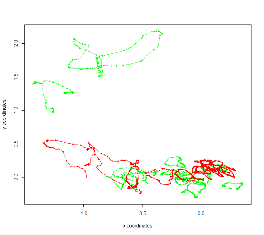
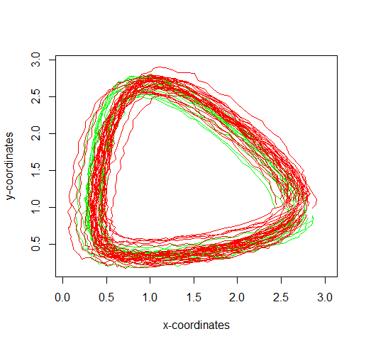
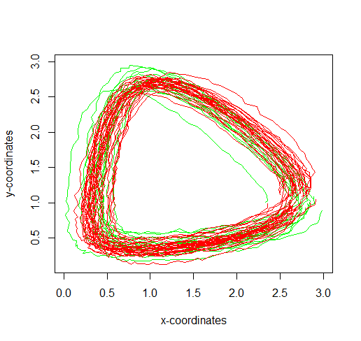
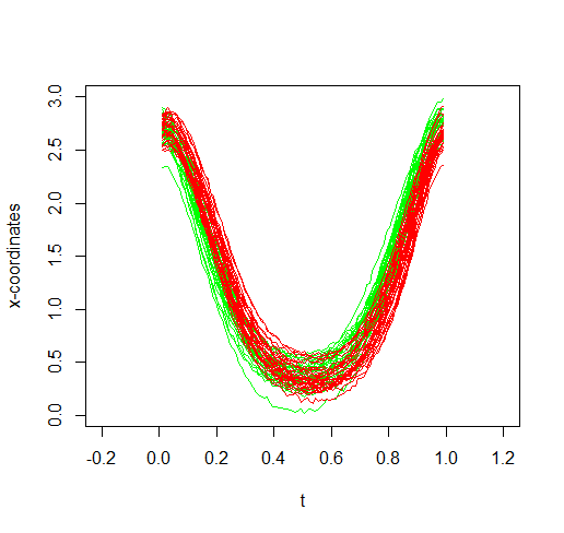
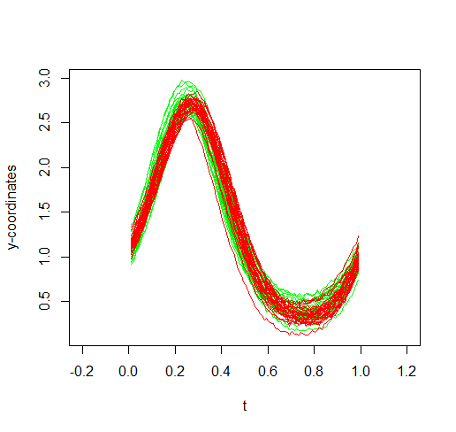
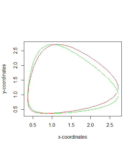
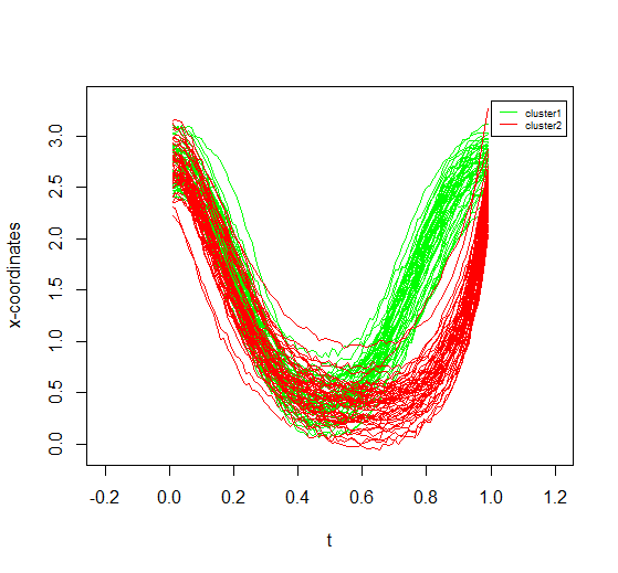
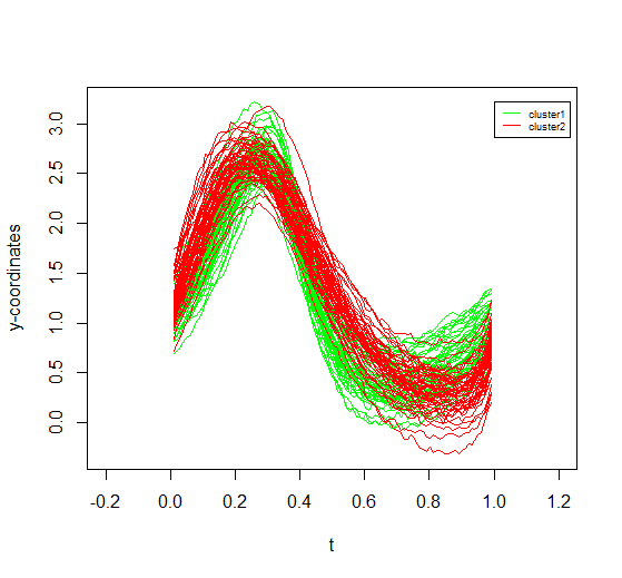
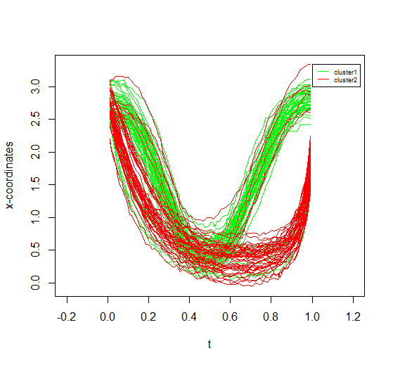
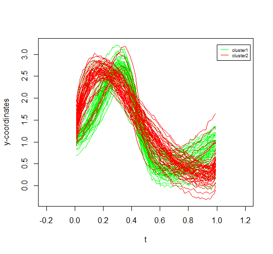
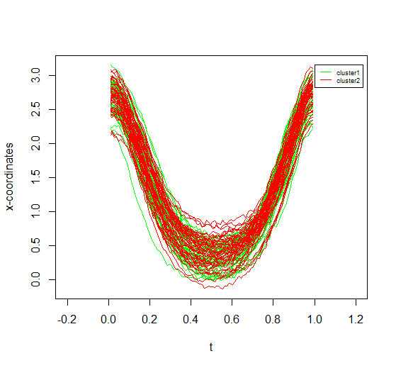
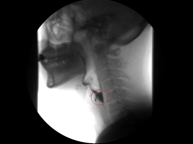
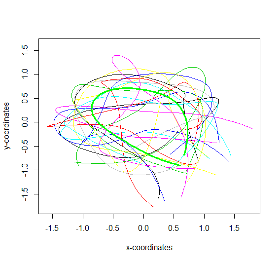
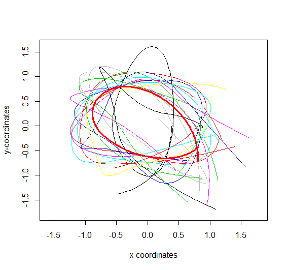
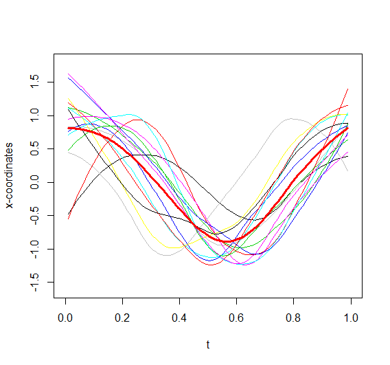
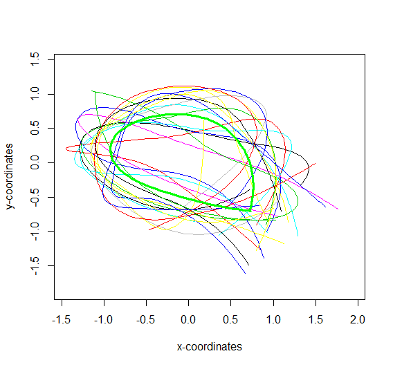
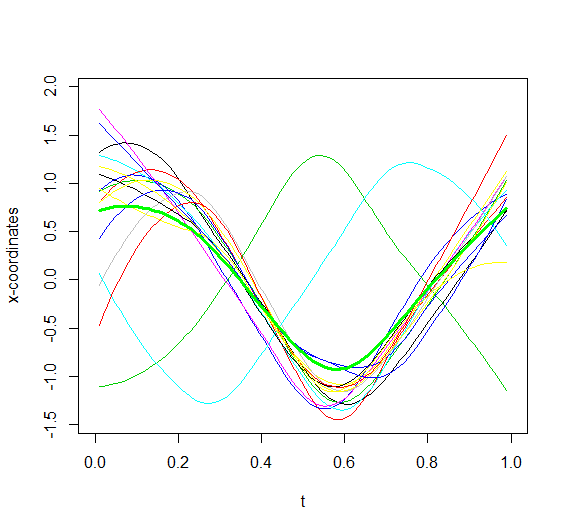
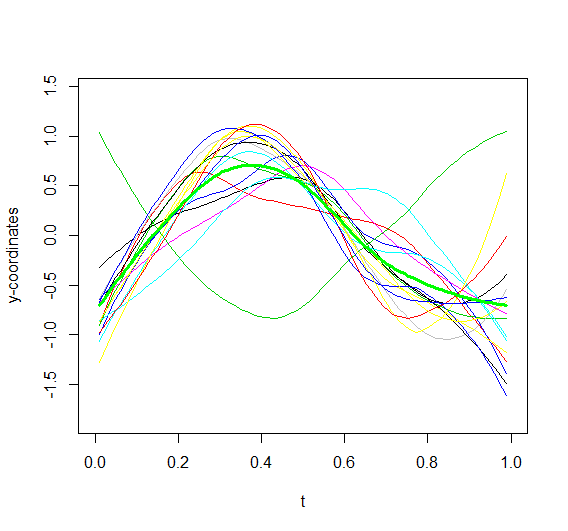
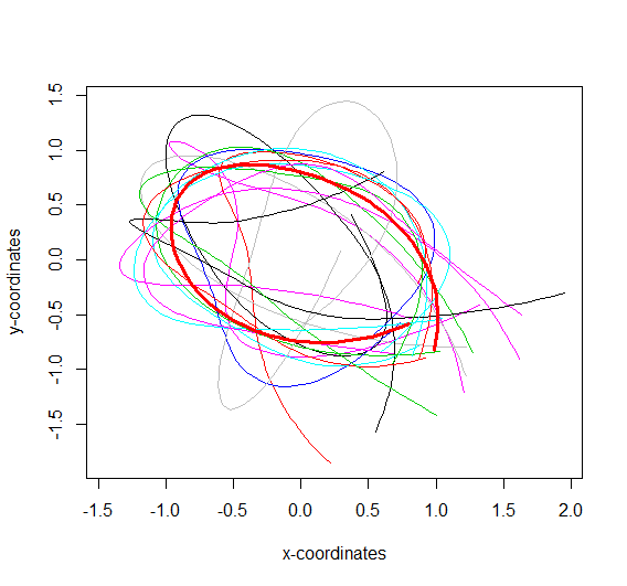
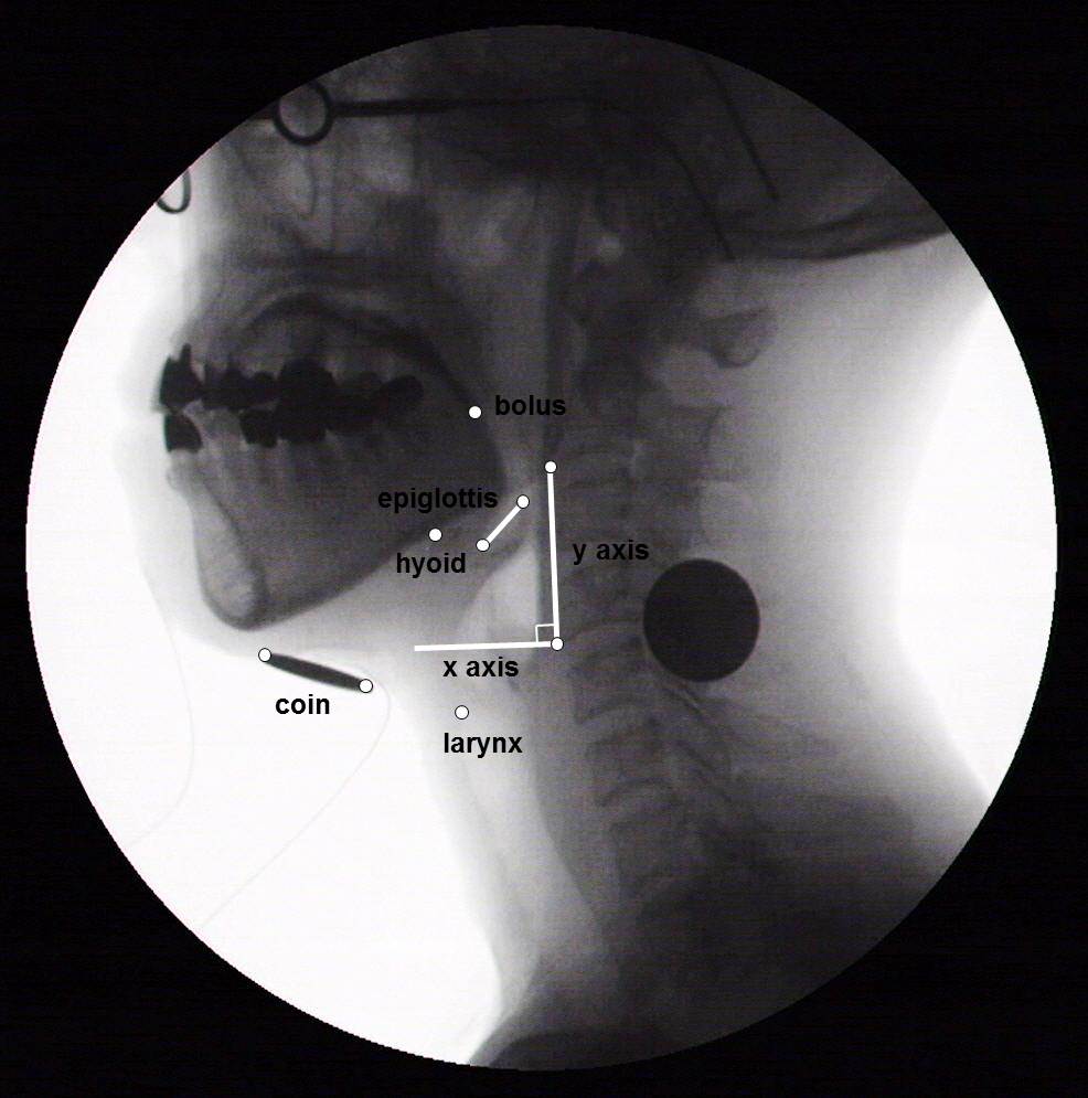
Figure 1: The motion data of hyoid bone. (𝐚𝐚\mathbf{a}) One X-ray image showing the location of hyoid bone which will move forward and backward to form one 2D curve during swallowing, as shown in (𝐛𝐛\mathbf{b}). (𝐛𝐛\mathbf{b}) 30 trajectories of hyoid bone motion from 15 normal people (curves in green) and 15 patients after stoke (curves in red).

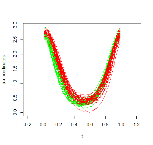
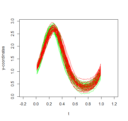
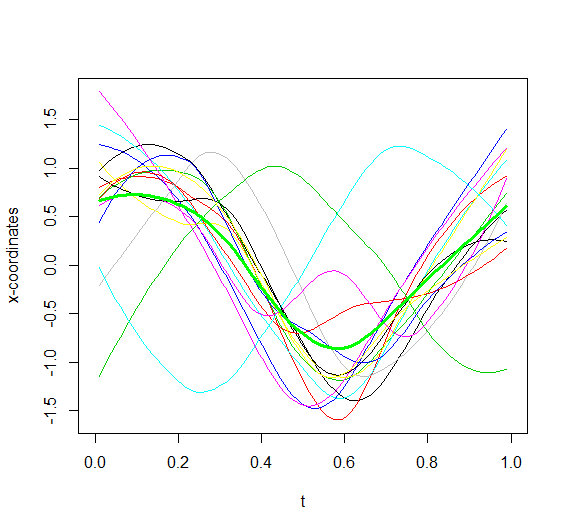
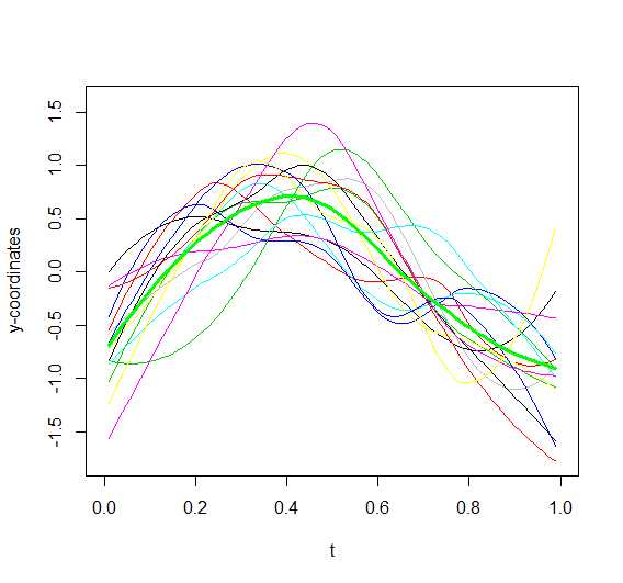
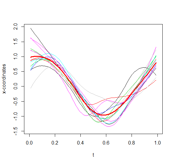
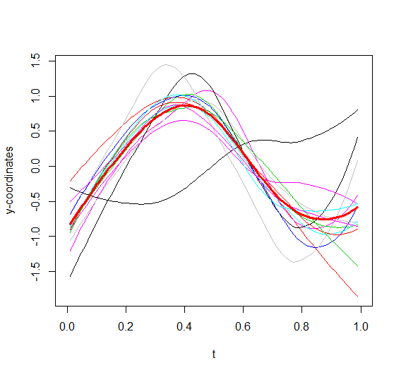
In our study of the motion analysis of hyoid bone observed from X-ray video clips, the trajectories can be thought of as 2D functional data (see Figure 1, the background of the data will be discussed in Section 3). There exists obvious misaligned problems for those curves in both vertical and horizontal variation. Usually, curve alignment is performed as a preprocessing technique and the clustering is conducted afterwards. This way is not efficient, since a subject belonging to which cluster is closely related to how it unfolds its progression pace. Another challenging problem for this study is that the heterogeneity of regression relationships among different groups. It consists in both the potential time warping for curves corresponding to the subjects and the subjects’ scalar variables such as initial level of disease, gender, age and the characteristics of those trajectories themselves, like motion time, average speed and range of motion. Therefore, simultaneous curve registration and clustering by considering all those factors seems to be a better way for modeling the functional data.

There are some research work on handling the similar problems. For instance, Liu and Yang, (2009) developed a framework that allows for simultaneously aligning and clustering k-centers functional data. But their model did not use any subject specific information (scalar variables) and assumed the heterogeneity among groups just depends on the curves themselves; similar idea is also used in k𝑘k-means alignment for curve clustering by Sangalli et al., (2010). On the other hand, Shi and Wang, (2008) proposed a hierarchical mixture of Gaussian process (GP) functional regression models with an allocation model to do curve prediction and clustering. They used the functional covariates to reconstruct the response curve and the personal scalar variables, such as height and gender, to deal with heterogeneity of the regression relationships among different groups. However, their method did not consider the misaligned problem. In addition, most related models are limited to one dimensional curve.

The purpose of our study is to address the above problems by constructing one hierarchical mixture of models for the sake of simultaneous curve registration and clustering. In the first level, we assume a simultaneous registration and functional regression model. And an allocation model with scalar variables is introduced as the second level model. Non-linear functional random effects are modeled by a GP in the first level model to address the heterogeneity among subjects. This also allows to estimate subject-specific warping function. The main contributions of this paper are: (i) simultaneously carrying out registration and modeling for multi-dimensional functional data (2D or 3D curves) allowing variation among subjects, and (ii) the use of both functional and scalar covariates while conducting clustering.

The paper is organized as follows. Section 2.1 defines simultaneous registration and clustering (SRC) models via two-level models. We discuss the estimation and the details of implementation in Section 2.2 and Section 2.3 respectively. The problem of model selection and the related methods are discussed in Section 2.4. Section 3 presents a number of examples with simulated data and real data. A short summary and discussion are given in Section 4.

2 The simultaneous registration and clustering method

Suppose there are N𝑁N subjects coming from K𝐾K different groups, 𝒙1,𝒙2,,𝒙Nsubscript𝒙1subscript𝒙2subscript𝒙𝑁\mbox{\boldmath${x}$}_{1},\mbox{\boldmath${x}$}_{2},\dots,\mbox{\boldmath${x}$}_{N} being the observations of 2D continuous curves, where 𝒙i=(𝒙1i(t),𝒙2i(t))subscript𝒙𝑖superscriptsubscript𝒙1𝑖𝑡subscript𝒙2𝑖𝑡\mbox{\boldmath${x}$}_{i}=(\mbox{\boldmath${x}$}_{1i}(t),\mbox{\boldmath${x}$}_{2i}(t))^{\intercal}, 𝒙1i(t)subscript𝒙1𝑖𝑡\mbox{\boldmath${x}$}_{1i}(t) and 𝒙2i(t)subscript𝒙2𝑖𝑡\mbox{\boldmath${x}$}_{2i}(t) are the corresponding x𝑥x-coordinates and y𝑦y-coordinates of 𝒙isubscript𝒙𝑖\mbox{\boldmath${x}$}_{i}. Let 𝒗1,,𝒗Nsubscript𝒗1subscript𝒗𝑁\mbox{\boldmath${v}$}_{1},\dots,\mbox{\boldmath${v}$}_{N} be the observed scalar variables. Suppose there are nisubscript𝑛𝑖n_{i} time points on which the i𝑖i-th curve is measured. The data set is

D={(𝒙i(tij),𝒗i);i=1,,N;j=1,,ni}.D=\{(\mbox{\boldmath${x}$}_{i}(t_{ij}),\mbox{\boldmath${v}$}_{i});i=1,\dots,N;j=1,\dots,n_{i}\}.

We introduce a latent indicator variable 𝒛i=(zi1,,ziK)subscript𝒛𝑖superscriptsubscript𝑧𝑖1subscript𝑧𝑖𝐾\mbox{\boldmath${z}$}_{i}=(z_{i1},\dots,z_{iK})^{\intercal} for the i𝑖i-th subject where ziksubscript𝑧𝑖𝑘z_{ik} takes value 111 if they are in the k𝑘k-th group and 00 otherwise.

2.1 The model

In our study of 2D curves, we will use the preprocessing procedure Generalized Procrustes Analysis (GPA) (Gower,, 1975) to address part of registration problems in advance except warping. Conventionally, most methods tried to complete all the registration problems including warping before clustering. This is not the best way since different warping functions may need to be used in different clusters, yet we have no such information before clustering, and heterogeneity among different subjects should also be considered. Thus, a hierarchical structure defined by two levels of models is proposed.

We start with the first level model for the continuous curve as follows

xai(t)|zki=1=(τakgki)(t)+raki(t)+ϵai(t),i=1,,N,formulae-sequenceevaluated-atsubscript𝑥𝑎𝑖𝑡subscript𝑧𝑘𝑖1subscript𝜏𝑎𝑘subscript𝑔𝑘𝑖𝑡subscript𝑟𝑎𝑘𝑖𝑡subscriptitalic-ϵ𝑎𝑖𝑡𝑖1𝑁x_{ai}(t)|_{z_{ki}=1}=(\tau_{ak}\circ g_{ki})(t)+r_{aki}(t)+\epsilon_{ai}(t),\hskip 14.22636pti=1,\dots,N, (1)

where a=1𝑎1a=1 or 2 represents x𝑥x- or y𝑦y-coordinates of 𝒙i(t)subscript𝒙𝑖𝑡\mbox{\boldmath${x}$}_{i}(t). The item (τakgki)subscript𝜏𝑎𝑘subscript𝑔𝑘𝑖(\tau_{ak}\circ g_{ki}) denotes functional composition: (τg)(t)=τ(g(t))𝜏𝑔𝑡𝜏𝑔𝑡(\tau\circ g)(t)=\tau(g(t)), where gki(t)subscript𝑔𝑘𝑖𝑡g_{ki}(t) is the inverse of a warping function. τak()subscript𝜏𝑎𝑘\tau_{ak}(\cdot) is a fixed but unknown nonlinear mean curve, which can be approximated by a set of basis functions, the details will be given in the next subsection. The variation among different subjects is modeled by a non-linear functional random-effects, raki(t)subscript𝑟𝑎𝑘𝑖𝑡r_{aki}(t), by a Gaussian process with zero-mean and a parametric covariance function S𝑆S (Shi et al.,, 2012). The error item ϵai(t)subscriptitalic-ϵ𝑎𝑖𝑡\epsilon_{ai}(t) is assumed to be Gaussian white noise with variance σ2superscript𝜎2\sigma^{2}.

Following the previous discussion, we need to use different warping function in different cluster, and we also need to consider the variation among different subjects, and thus, we allow warping function depending on k𝑘k and i𝑖i. Further, we assume

gki(t)=t+wk(t)+wki(t),subscript𝑔𝑘𝑖𝑡𝑡subscript𝑤𝑘𝑡subscript𝑤𝑘𝑖𝑡g_{ki}(t)=t+w_{k}(t)+w_{ki}(t),

where wk(t)subscript𝑤𝑘𝑡w_{k}(t) is the fixed part and wki(t)subscript𝑤𝑘𝑖𝑡w_{ki}(t) is the random part in terms of different subjects. Instead of making assumption for curves wk(t)subscript𝑤𝑘𝑡w_{k}(t) and wki(t)subscript𝑤𝑘𝑖𝑡w_{ki}(t), we first discretize them by a set of fixed parameters, for example, by 𝒘k=(wk(t1),,wk(tnv))subscript𝒘𝑘subscript𝑤𝑘subscript𝑡1subscript𝑤𝑘subscript𝑡subscript𝑛𝑣\mbox{\boldmath${w}$}_{k}=(w_{k}(t_{1}),\dots,w_{k}(t_{n_{v}})) and 𝒘ki=(wki(t1),,wki(tnw))subscript𝒘𝑘𝑖subscript𝑤𝑘𝑖subscript𝑡1subscript𝑤𝑘𝑖subscript𝑡subscript𝑛𝑤\mbox{\boldmath${w}$}_{ki}=(w_{ki}(t_{1}),\dots,w_{ki}(t_{n_{w}})) respectively. We then model 𝒘kisubscript𝒘𝑘𝑖\mbox{\boldmath${w}$}_{ki} by a Gaussian distribution with zero mean and a parametric covariance function 𝑯𝑯{H}. We can also define the warping function as simple as a horizontal shift, i.e. gki(t)=t+bkisubscript𝑔𝑘𝑖𝑡𝑡subscript𝑏𝑘𝑖g_{ki}(t)=t+b_{ki} or a linear stretch of the curves, i.e. gki(t)=(1+bki)t+ckisubscript𝑔𝑘𝑖𝑡1subscript𝑏𝑘𝑖𝑡subscript𝑐𝑘𝑖g_{ki}(t)=(1+b_{ki})t+c_{ki}, where bkisubscript𝑏𝑘𝑖b_{ki} and ckisubscript𝑐𝑘𝑖c_{ki} are both one dimensional unknown parameter. Those linear warping functions have been examined by others (Liu and Yang,, 2009; Sangalli et al.,, 2010).

We define a logistic allocation model in the second level model for the latent indicator variable in the form

p(zki=1)=πki=exp{𝒗i𝜷k}1+j=1K1exp{𝒗i𝜷j},i=1,,N;k=1,,K1,formulae-sequence𝑝subscript𝑧𝑘𝑖1subscript𝜋𝑘𝑖expsubscriptsuperscript𝒗𝑖subscript𝜷𝑘1superscriptsubscript𝑗1𝐾1expsubscriptsuperscript𝒗𝑖subscript𝜷𝑗formulae-sequence𝑖1𝑁𝑘1𝐾1p(z_{ki}=1)=\pi_{ki}=\frac{\text{exp}\{\mbox{\boldmath${v}$}^{\intercal}_{i}\mbox{\boldmath${\beta}$}_{k}\}}{1+\sum_{j=1}^{K-1}\text{exp}\{\mbox{\boldmath${v}$}^{\intercal}_{i}\mbox{\boldmath${\beta}$}_{j}\}},\hskip 14.22636pti=1,\dots,N;\hskip 14.22636ptk=1,\dots,K-1, (2)

with p(zKi=1)=πKi=1l=1K1πli𝑝subscript𝑧𝐾𝑖1subscript𝜋𝐾𝑖1superscriptsubscript𝑙1𝐾1subscript𝜋𝑙𝑖p(z_{Ki}=1)=\pi_{Ki}=1-\sum_{l=1}^{K-1}\pi_{li}, where {𝜷k,k=1,,K1}formulae-sequencesubscript𝜷𝑘𝑘1𝐾1\{\bm{\beta}_{k},k=1,\dots,K-1\} are unknown parameters to be estimated. We can also replace model (2) by other models, e.g. Potts model (Green and Richardson,, 2000). The information of scalar variables is integrated with functional variables via the two-level models (1) and (2). The reason of using both types of variables is that the variation between subjects does not usually depend on the curve data only, summary statistics or some subject-specific variables do provide useful information, like the scenario in Figure A.4 and Figure A.5 in the simulated example and Table 2 and Figure A.9 in the real data analysis. The introduction of the latent indicator variable is very useful in the implementation; see the details below.

We call the models defined in (1) and (2) as simultaneous registration and clustering (SRC) models.

2.2 Estimation

The discrete form of model (1) for the i𝑖ith curve data 𝐱ai=(xai(ti1),,xai(tini))subscript𝐱𝑎𝑖superscriptsubscript𝑥𝑎𝑖subscript𝑡𝑖1subscript𝑥𝑎𝑖subscript𝑡𝑖subscript𝑛𝑖\mathbf{x}_{ai}=\big{(}x_{ai}(t_{i1}),\dots,x_{ai}(t_{in_{i}})\big{)}^{\intercal} can be expressed as follows

𝒙ai|zki=1=𝝉ak(gki)+𝒓aki+ϵi,fora=1,2;k=1,,K,formulae-sequenceevaluated-atsubscript𝒙𝑎𝑖subscript𝑧𝑘𝑖1subscript𝝉𝑎𝑘subscript𝑔𝑘𝑖subscript𝒓𝑎𝑘𝑖subscriptbold-italic-ϵ𝑖formulae-sequencefor𝑎12𝑘1𝐾\mbox{\boldmath${x}$}_{ai}|_{z_{ki}=1}=\mbox{\boldmath${\tau}$}_{ak}(g_{ki})+\mbox{\boldmath${r}$}_{aki}+\mbox{\boldmath${\epsilon}$}_{i},\hskip 14.22636pt\text{for}\hskip 5.69054pta=1,2;\hskip 5.69054ptk=1,\dots,K, (3)

where 𝝉ak(gki)=(τak(gki(ti1)),,τak(gki(tini)))subscript𝝉𝑎𝑘subscript𝑔𝑘𝑖superscriptsubscript𝜏𝑎𝑘subscript𝑔𝑘𝑖subscript𝑡𝑖1subscript𝜏𝑎𝑘subscript𝑔𝑘𝑖subscript𝑡𝑖subscript𝑛𝑖\mbox{\boldmath${\tau}$}_{ak}(g_{ki})=\Big{(}\tau_{ak}\big{(}g_{ki}(t_{i1})\big{)},\dots,\tau_{ak}\big{(}g_{ki}(t_{in_{i}})\big{)}\Big{)}^{\intercal}, and 𝒓akisubscript𝒓𝑎𝑘𝑖\mbox{\boldmath${r}$}_{aki} and ϵisubscriptbold-italic-ϵ𝑖\mbox{\boldmath${\epsilon}$}_{i} are both nisubscript𝑛𝑖n_{i}-dimensional column vector. In this paper, we respectively set 𝑺𝑺{S} as the Matern covariance function with parameters 𝝆ssubscript𝝆𝑠\mbox{\boldmath${\rho}$}_{s} and 𝑯𝑯{H} as the unstructured covariance function or Brownian covariance function with parameter 𝝆hsubscript𝝆\mbox{\boldmath${\rho}$}_{h} (Raket,, 2016), and they can be estimated by the data; the details are provided in the next subsection. Other covariance functions can also be used (Shi and Choi,, 2011). Let 𝑺akisubscript𝑺𝑎𝑘𝑖\mbox{\boldmath${S}$}_{aki} and 𝑯kisubscript𝑯𝑘𝑖\mbox{\boldmath${H}$}_{ki} be the covariance matrix of 𝒓akisubscript𝒓𝑎𝑘𝑖\mbox{\boldmath${r}$}_{aki} and 𝒘kisubscript𝒘𝑘𝑖\mbox{\boldmath${w}$}_{ki} respectively, which can be calculated by the corresponding covariance function. We model τak(t)subscript𝜏𝑎𝑘𝑡\tau_{ak}(t) using q𝑞q basis functions {ψ1(t),,ψq(t)}subscript𝜓1𝑡subscript𝜓𝑞𝑡\{\psi_{1}(t),\dots,\psi_{q}(t)\} with weights 𝒅ak=(dak1,,dakq)subscript𝒅𝑎𝑘superscriptsubscript𝑑𝑎𝑘1subscript𝑑𝑎𝑘𝑞\mbox{\boldmath${d}$}_{ak}=(d_{ak1},\dots,d_{akq})^{\intercal}. Thus, 𝝉ak(gki)=𝚿ki𝒅aksubscript𝝉𝑎𝑘subscript𝑔𝑘𝑖subscript𝚿𝑘𝑖subscript𝒅𝑎𝑘\mbox{\boldmath${\tau}$}_{ak}(g_{ki})=\mbox{\boldmath${\Psi}$}_{ki}\mbox{\boldmath${d}$}_{ak} where 𝚿ki=[𝚿ki1,,𝚿kiq]ni×q,𝚿kil=(ψl(gki(ti1)),,ψl(gki(tini))),l=1,,qformulae-sequencesubscript𝚿𝑘𝑖subscriptsubscript𝚿𝑘𝑖1subscript𝚿𝑘𝑖𝑞subscript𝑛𝑖𝑞formulae-sequencesubscript𝚿𝑘𝑖𝑙superscriptsubscript𝜓𝑙subscript𝑔𝑘𝑖subscript𝑡𝑖1subscript𝜓𝑙subscript𝑔𝑘𝑖subscript𝑡𝑖subscript𝑛𝑖𝑙1𝑞\mbox{\boldmath${\Psi}$}_{ki}=[\mbox{\boldmath${\Psi}$}_{ki1},\dots,\mbox{\boldmath${\Psi}$}_{kiq}]_{n_{i}\times q},\mbox{\boldmath${\Psi}$}_{kil}=(\psi_{l}(g_{ki}(t_{i1})),\dots,\psi_{l}(g_{ki}(t_{in_{i}})))^{\intercal},l=1,\dots,q. In this paper, we use a smooth non-linear deformation for the curves, which is produced by a cubic Hermite spline (Raket,, 2016).

The unknown parameters from the k𝑘k-th component for the a𝑎a-coordinates (x𝑥x- or y𝑦y-coordinates) of the i𝑖i-th curve are denoted by 𝜽aki=Δ{𝒅ak,𝒘k,𝒘ki,𝝆s,𝝆h,σ}subscript𝜽𝑎𝑘𝑖Δsubscript𝒅𝑎𝑘subscript𝒘𝑘subscript𝒘𝑘𝑖subscript𝝆𝑠subscript𝝆𝜎\mbox{\boldmath${\theta}$}_{aki}\overset{\Delta}{=}\{\mbox{\boldmath${d}$}_{ak},\mbox{\boldmath${w}$}_{k},\mbox{\boldmath${w}$}_{ki},\mbox{\boldmath${\rho}$}_{s},\mbox{\boldmath${\rho}$}_{h},\sigma\}. Let 𝜽kisubscript𝜽𝑘𝑖\mbox{\boldmath${\theta}$}_{ki} be the vector of {𝜽aki,a=1,2}formulae-sequencesubscript𝜽𝑎𝑘𝑖𝑎12\{\mbox{\boldmath${\theta}$}_{aki},a=1,2\}. We can similarly define 𝜽i={𝜽ki,k=1,,K}\mbox{\boldmath${\theta}$}_{i}=\{\mbox{\boldmath${\theta}$}_{ki},k=1,\dots,K\}, 𝜽={𝜽i,i=1,,N}\mbox{\boldmath${\theta}$}=\{\mbox{\boldmath${\theta}$}_{i},i=1,\dots,N\} and 𝜷={𝜷k,k=1,,K1}\mbox{\boldmath${\beta}$}=\{\mbox{\boldmath${\beta}$}_{k},k=1,\dots,K-1\}. The Gaussian mixture distribution for the i𝑖i-th curve data can be written in the form

p(𝒙i|𝜽i,𝜷)=k=1Kπkip(𝒙i|𝜽ki),i=1,,N,formulae-sequence𝑝conditionalsubscript𝒙𝑖subscript𝜽𝑖𝜷superscriptsubscript𝑘1𝐾subscript𝜋𝑘𝑖𝑝conditionalsubscript𝒙𝑖subscript𝜽𝑘𝑖𝑖1𝑁p(\mbox{\boldmath${x}$}_{i}|\mbox{\boldmath${\theta}$}_{i},\mbox{\boldmath${\beta}$})=\sum_{k=1}^{K}\pi_{ki}p(\mbox{\boldmath${x}$}_{i}|\mbox{\boldmath${\theta}$}_{ki}),\hskip 14.22636pti=1,\dots,N,

where p(𝒙i|𝜽ki)=p(𝒙1i|𝜽1ki)p(𝒙2i|𝜽2ki)𝑝conditionalsubscript𝒙𝑖subscript𝜽𝑘𝑖𝑝conditionalsubscript𝒙1𝑖subscript𝜽1𝑘𝑖𝑝conditionalsubscript𝒙2𝑖subscript𝜽2𝑘𝑖p(\mbox{\boldmath${x}$}_{i}|\mbox{\boldmath${\theta}$}_{ki})=p(\mbox{\boldmath${x}$}_{1i}|\mbox{\boldmath${\theta}$}_{1ki})p(\mbox{\boldmath${x}$}_{2i}|\mbox{\boldmath${\theta}$}_{2ki}). We assume 𝒙1isubscript𝒙1𝑖\mbox{\boldmath${x}$}_{1i} and 𝒙2isubscript𝒙2𝑖\mbox{\boldmath${x}$}_{2i} are conditional independent given those parameters. The log-likelihood of (𝜽,𝜷)𝜽𝜷(\mbox{\boldmath${\theta}$},\mbox{\boldmath${\beta}$}) is therefore

L(𝜽,𝜷)=i=1Nlog{k=1Kπkip(𝒙i|𝜽ki)}.𝐿𝜽𝜷superscriptsubscript𝑖1𝑁logsuperscriptsubscript𝑘1𝐾subscript𝜋𝑘𝑖𝑝conditionalsubscript𝒙𝑖subscript𝜽𝑘𝑖L(\mbox{\boldmath${\theta}$},\mbox{\boldmath${\beta}$})=\sum_{i=1}^{N}\text{log}\Big{\{}\sum_{k=1}^{K}\pi_{ki}p(\mbox{\boldmath${x}$}_{i}|\mbox{\boldmath${\theta}$}_{ki})\Big{\}}.

It is quite tricky to conduct the estimation due to the large number of unknown parameters. EM algorithm will be adopted in this paper. We have defined the latent indicator variable 𝒛isubscript𝒛𝑖\mbox{\boldmath${z}$}_{i}, which is treated as missing. The joint likelihood function of 𝒙𝒙{x} and 𝒛𝒛{z}, where 𝒛={𝒛i;i=1,,N}\mbox{\boldmath${z}$}=\{\mbox{\boldmath${z}$}_{i};i=1,\dots,N\}, takes the form

p(𝒙,𝒛|𝜽,𝜷)=p(𝒛|𝜷)p(𝒙|𝒛,𝜽)=i=1Nk=1Kπkizkip(𝒙i|𝜽ki)zki.𝑝𝒙conditional𝒛𝜽𝜷𝑝conditional𝒛𝜷𝑝conditional𝒙𝒛𝜽superscriptsubscriptproduct𝑖1𝑁superscriptsubscriptproduct𝑘1𝐾superscriptsubscript𝜋𝑘𝑖subscript𝑧𝑘𝑖𝑝superscriptconditionalsubscript𝒙𝑖subscript𝜽𝑘𝑖subscript𝑧𝑘𝑖p(\mbox{\boldmath${x}$},\mbox{\boldmath${z}$}|\mbox{\boldmath${\theta}$},\mbox{\boldmath${\beta}$})=p(\mbox{\boldmath${z}$}|\mbox{\boldmath${\beta}$})p(\mbox{\boldmath${x}$}|\mbox{\boldmath${z}$},\mbox{\boldmath${\theta}$})=\prod_{i=1}^{N}\prod_{k=1}^{K}\pi_{ki}^{z_{ki}}p(\mbox{\boldmath${x}$}_{i}|\mbox{\boldmath${\theta}$}_{ki})^{z_{ki}}.

Taking the logarithm, we have the log-likelihood for complete data (𝒙,𝒛)𝒙𝒛(\mbox{\boldmath${x}$},\mbox{\boldmath${z}$})

Lc(𝜽,𝜷)=logp(𝒙,𝒛|𝜽,𝜷)=i=1Nk=1Kzki(logπki+logp(𝒙i|𝜽ki)).subscript𝐿𝑐𝜽𝜷log𝑝𝒙conditional𝒛𝜽𝜷superscriptsubscript𝑖1𝑁superscriptsubscript𝑘1𝐾subscript𝑧𝑘𝑖logsubscript𝜋𝑘𝑖log𝑝conditionalsubscript𝒙𝑖subscript𝜽𝑘𝑖\displaystyle L_{c}(\mbox{\boldmath${\theta}$},\mbox{\boldmath${\beta}$})=\text{log}p(\mbox{\boldmath${x}$},\mbox{\boldmath${z}$}|\mbox{\boldmath${\theta}$},\mbox{\boldmath${\beta}$})=\sum_{i=1}^{N}\sum_{k=1}^{K}z_{ki}\bigg{(}\text{log}\pi_{ki}+\text{log}p(\mbox{\boldmath${x}$}_{i}|\mbox{\boldmath${\theta}$}_{ki})\bigg{)}. (4)

The expected value of the complete log-likelihood with respect to 𝒛𝒛{z} is given by

E𝒛{Lc(𝜽,𝜷)}=k=1Ki=1NE(zki|𝒙,𝜽,𝜷)(logπki+logp(𝒙i|𝜽ki))=k=1Ki=1NMki(logπki+logp(𝒙i|𝜽ki)),subscript𝐸𝒛subscript𝐿𝑐𝜽𝜷superscriptsubscript𝑘1𝐾superscriptsubscript𝑖1𝑁𝐸conditionalsubscript𝑧𝑘𝑖𝒙𝜽𝜷logsubscript𝜋𝑘𝑖log𝑝conditionalsubscript𝒙𝑖subscript𝜽𝑘𝑖superscriptsubscript𝑘1𝐾superscriptsubscript𝑖1𝑁subscript𝑀𝑘𝑖logsubscript𝜋𝑘𝑖log𝑝conditionalsubscript𝒙𝑖subscript𝜽𝑘𝑖{}\begin{split}E_{\mbox{\boldmath${z}$}}\{L_{c}(\mbox{\boldmath${\theta}$},\mbox{\boldmath${\beta}$})\}&=\sum_{k=1}^{K}\sum_{i=1}^{N}E(z_{ki}|\mbox{\boldmath${x}$},\mbox{\boldmath${\theta}$},\mbox{\boldmath${\beta}$})\bigg{(}\text{log}\pi_{ki}+\text{log}p(\mbox{\boldmath${x}$}_{i}|\mbox{\boldmath${\theta}$}_{ki})\bigg{)}\\ &=\sum_{k=1}^{K}\sum_{i=1}^{N}M_{ki}\bigg{(}\text{log}\pi_{ki}+\text{log}p(\mbox{\boldmath${x}$}_{i}|\mbox{\boldmath${\theta}$}_{ki})\bigg{)},\end{split} (5)

where

Mki=ΔE(zki|𝒙,𝜽,𝜷)=πkip(𝒙i|𝜽ki)j=1Kπjip(𝒙i|𝜽ji),i=1,,N;k=1,,K.formulae-sequencesubscript𝑀𝑘𝑖Δ𝐸conditionalsubscript𝑧𝑘𝑖𝒙𝜽𝜷subscript𝜋𝑘𝑖𝑝conditionalsubscript𝒙𝑖subscript𝜽𝑘𝑖superscriptsubscript𝑗1𝐾subscript𝜋𝑗𝑖𝑝conditionalsubscript𝒙𝑖subscript𝜽𝑗𝑖formulae-sequence𝑖1𝑁𝑘1𝐾M_{ki}\overset{\Delta}{=}E(z_{ki}|\mbox{\boldmath${x}$},\mbox{\boldmath${\theta}$},\mbox{\boldmath${\beta}$})=\frac{\pi_{ki}p(\mbox{\boldmath${x}$}_{i}|\mbox{\boldmath${\theta}$}_{ki})}{\sum_{j=1}^{K}\pi_{ji}p(\mbox{\boldmath${x}$}_{i}|\mbox{\boldmath${\theta}$}_{ji})},\hskip 14.22636pti=1,\dots,N;k=1,\dots,K.

The derivation of Mkisubscript𝑀𝑘𝑖M_{ki} is given by Appendix 1. The procedure of EM algorithm includes

  1. 1.

    Initialize 𝜽(l)superscript𝜽𝑙\mbox{\boldmath${\theta}$}^{(l)} and 𝜷(l)superscript𝜷𝑙\mbox{\boldmath${\beta}$}^{(l)} and evaluate the Mkisubscript𝑀𝑘𝑖M_{ki} (E-step)

    Mki=πki(l)p(𝒙i|𝜽ki(l))j=1Kπji(l)p(𝒙i|𝜽ji(l)).subscript𝑀𝑘𝑖superscriptsubscript𝜋𝑘𝑖𝑙𝑝conditionalsubscript𝒙𝑖subscriptsuperscript𝜽𝑙𝑘𝑖superscriptsubscript𝑗1𝐾superscriptsubscript𝜋𝑗𝑖𝑙𝑝conditionalsubscript𝒙𝑖subscriptsuperscript𝜽𝑙𝑗𝑖M_{ki}=\frac{\pi_{ki}^{(l)}p(\mbox{\boldmath${x}$}_{i}|\mbox{\boldmath${\theta}$}^{(l)}_{ki})}{\sum_{j=1}^{K}\pi_{ji}^{(l)}p(\mbox{\boldmath${x}$}_{i}|\mbox{\boldmath${\theta}$}^{(l)}_{ji})}.
  2. 2.

    Fix Mkisubscript𝑀𝑘𝑖M_{ki} and maximize Q(𝜽,𝜷)𝑄𝜽𝜷Q(\mbox{\boldmath${\theta}$},\mbox{\boldmath${\beta}$}) with respect to 𝜽𝜽{\theta} and 𝜷𝜷{\beta}

    Q(𝜽,𝜷)=Δk=1Ki=1NMki(logπki+logp(𝒙i|𝜽ki)),𝑄𝜽𝜷Δsuperscriptsubscript𝑘1𝐾superscriptsubscript𝑖1𝑁subscript𝑀𝑘𝑖logsubscript𝜋𝑘𝑖log𝑝conditionalsubscript𝒙𝑖subscript𝜽𝑘𝑖Q(\mbox{\boldmath${\theta}$},\mbox{\boldmath${\beta}$})\overset{\Delta}{=}\sum_{k=1}^{K}\sum_{i=1}^{N}M_{ki}\bigg{(}\text{log}\pi_{ki}+\text{log}p(\mbox{\boldmath${x}$}_{i}|\mbox{\boldmath${\theta}$}_{ki})\bigg{)},

    leading to 𝜽(l+1)superscript𝜽𝑙1\mbox{\boldmath${\theta}$}^{(l+1)} and 𝜷(l+1)superscript𝜷𝑙1\mbox{\boldmath${\beta}$}^{(l+1)} (M-step).

The technical details are given in the next subsection.

2.3 Implementation

In E-step, we first initialize the weights Mkisubscript𝑀𝑘𝑖M_{ki}. In practice, we choose Mki(0)U(0,1)similar-tosuperscriptsubscript𝑀𝑘𝑖0𝑈01M_{ki}^{(0)}\sim U(0,1) for the purpose of simplicity. Each Mkisubscript𝑀𝑘𝑖M_{ki} is then divided by their summation k=1KMkisuperscriptsubscript𝑘1𝐾subscript𝑀𝑘𝑖\sum_{k=1}^{K}M_{ki} and we set πki(0)=Mki(0)subscriptsuperscript𝜋0𝑘𝑖superscriptsubscript𝑀𝑘𝑖0\pi^{(0)}_{ki}=M_{ki}^{(0)}. In M-step, there are no analytic solutions to the maximization of Q(𝜽,𝜷)𝑄𝜽𝜷Q(\mbox{\boldmath${\theta}$},\mbox{\boldmath${\beta}$}) with respect to 𝜽𝜽{\theta}, so that we use the following algorithms. Maximizing Q(𝜽,𝜷)𝑄𝜽𝜷Q(\mbox{\boldmath${\theta}$},\mbox{\boldmath${\beta}$}) with respect to 𝜽𝜽{\theta} given the current weights Miksubscript𝑀𝑖𝑘M_{ik} is equivalent to maximizing

k=1Ki=1NMki(a=12(logp(𝒙ai|𝜽aki))).superscriptsubscript𝑘1𝐾superscriptsubscript𝑖1𝑁subscript𝑀𝑘𝑖superscriptsubscript𝑎12log𝑝conditionalsubscript𝒙𝑎𝑖subscript𝜽𝑎𝑘𝑖\sum_{k=1}^{K}\sum_{i=1}^{N}M_{ki}\bigg{(}\sum_{a=1}^{2}\big{(}\text{log}p(\mbox{\boldmath${x}$}_{ai}|\mbox{\boldmath${\theta}$}_{aki})\big{)}\bigg{)}.

Borrowing the idea from Raket et al., (2016), all the parameters within 𝜽𝜽{\theta} are estimated iteratively through three conditional models. In order to simplify the likelihood computations, all the random effects are scaled by a noise standard deviation σ𝜎\sigma. The norm induced by a full-rank covariance matrix 𝑩𝑩{B} is denoted by 𝑨𝑩2=𝑨T𝑩1𝑨subscriptsuperscriptnorm𝑨2𝑩superscript𝑨𝑇superscript𝑩1𝑨||\mbox{\boldmath${A}$}||^{2}_{\mbox{\boldmath${B}$}}=\mbox{\boldmath${A}$}^{T}\mbox{\boldmath${B}$}^{-1}\mbox{\boldmath${A}$}.

(i) Estimating the fixed effects τaksubscript𝜏𝑎𝑘\mbox{\boldmath${\tau}$}_{ak}

Given 𝜽(l)superscript𝜽𝑙\mbox{\boldmath${\theta}$}^{(l)}, we have 𝒙ai|zki=1Nni(𝚿ki𝒅ak,𝑰ni+𝑺aki),a=1,2;i=1,,Nformulae-sequencesimilar-toevaluated-atsubscript𝒙𝑎𝑖subscript𝑧𝑘𝑖1subscript𝑁subscript𝑛𝑖subscript𝚿𝑘𝑖subscript𝒅𝑎𝑘subscript𝑰subscript𝑛𝑖subscript𝑺𝑎𝑘𝑖formulae-sequence𝑎12𝑖1𝑁\mbox{\boldmath${x}$}_{ai}|_{z_{ki}=1}\sim N_{n_{i}}(\mbox{\boldmath${\Psi}$}_{ki}\mbox{\boldmath${d}$}_{ak},\mbox{\boldmath${I}$}_{n_{i}}+\mbox{\boldmath${S}$}_{aki}),a=1,2;i=1,\dots,N. 𝑰nisubscript𝑰subscript𝑛𝑖\mbox{\boldmath${I}$}_{n_{i}} denotes the ni×nisubscript𝑛𝑖subscript𝑛𝑖n_{i}\times n_{i} identity matrix. So the negative log likelihood for the weights 𝒅aksubscript𝒅𝑎𝑘\mbox{\boldmath${d}$}_{ak} (its square magnitude is penalized by a weighting factor η𝜂\eta) is proportional to

L(𝒅ak)=i=1NMki𝒙ai𝚿ki𝒅ak𝑰ni+𝑺aki2+η𝒅ak𝒅ak,a=1,2;k=1,,K.formulae-sequence𝐿subscript𝒅𝑎𝑘superscriptsubscript𝑖1𝑁subscript𝑀𝑘𝑖subscriptsuperscriptnormsubscript𝒙𝑎𝑖subscript𝚿𝑘𝑖subscript𝒅𝑎𝑘2subscript𝑰subscript𝑛𝑖subscript𝑺𝑎𝑘𝑖𝜂superscriptsubscript𝒅𝑎𝑘subscript𝒅𝑎𝑘formulae-sequence𝑎12𝑘1𝐾L(\mbox{\boldmath${d}$}_{ak})=\sum_{i=1}^{N}M_{ki}||\mbox{\boldmath${x}$}_{ai}-\mbox{\boldmath${\Psi}$}_{ki}\mbox{\boldmath${d}$}_{ak}||^{2}_{\mbox{\boldmath${I}$}_{n_{i}}+\mbox{\boldmath${S}$}_{aki}}+\eta\mbox{\boldmath${d}$}_{ak}^{\intercal}\mbox{\boldmath${d}$}_{ak},\hskip 14.22636pta=1,2;\hskip 14.22636ptk=1,\dots,K.

This gives the estimator

𝒅^ak=(𝚿k(𝑰n+𝑺ak𝑴k)1𝚿k+η𝑰q)1𝚿k(𝑰n+𝑺ak𝑴k)1𝒙a,a=1,2;k=1,,K,formulae-sequencesubscript^𝒅𝑎𝑘superscriptsuperscriptsubscript𝚿𝑘superscriptsubscript𝑰𝑛subscript𝑺𝑎𝑘subscript𝑴𝑘1subscript𝚿𝑘𝜂subscript𝑰𝑞1superscriptsubscript𝚿𝑘superscriptsubscript𝑰𝑛subscript𝑺𝑎𝑘subscript𝑴𝑘1subscript𝒙𝑎formulae-sequence𝑎12𝑘1𝐾\hat{\mbox{\boldmath${d}$}}_{ak}=(\mbox{\boldmath${\Psi}$}_{k}^{\intercal}(\frac{\mbox{\boldmath${I}$}_{n}+\mbox{\boldmath${S}$}_{ak}}{\mbox{\boldmath${M}$}_{k}})^{-1}\mbox{\boldmath${\Psi}$}_{k}+\eta\mbox{\boldmath${I}$}_{q})^{-1}\mbox{\boldmath${\Psi}$}_{k}^{\intercal}(\frac{\mbox{\boldmath${I}$}_{n}+\mbox{\boldmath${S}$}_{ak}}{\mbox{\boldmath${M}$}_{k}})^{-1}\mbox{\boldmath${x}$}_{a},\hskip 14.22636pta=1,2;\hskip 14.22636ptk=1,\dots,K,

where 𝚿k=[𝚿k1,,𝚿kN]𝑹m×qsubscript𝚿𝑘superscriptsuperscriptsubscript𝚿𝑘1superscriptsubscript𝚿𝑘𝑁superscript𝑹𝑚𝑞\mbox{\boldmath${\Psi}$}_{k}=[\mbox{\boldmath${\Psi}$}_{k1}^{\intercal},\dots,\mbox{\boldmath${\Psi}$}_{kN}^{\intercal}]^{\intercal}\in\mbox{\boldmath${R}$}^{m\times q}, m=i=1Nni𝑚superscriptsubscript𝑖1𝑁subscript𝑛𝑖m=\sum_{i=1}^{N}n_{i}, 𝒙a=(𝒙a1,,𝒙aN)subscript𝒙𝑎superscriptsuperscriptsubscript𝒙𝑎1superscriptsubscript𝒙𝑎𝑁\mbox{\boldmath${x}$}_{a}=(\mbox{\boldmath${x}$}_{a1}^{\intercal},\dots,\mbox{\boldmath${x}$}_{aN}^{\intercal})^{\intercal} and

𝑰n+𝑺ak𝑴k=Δ[(𝑰n1+𝑺ak1)/Mk1(𝑰nN+𝑺akN)/MkN]m×m.subscript𝑰𝑛subscript𝑺𝑎𝑘subscript𝑴𝑘Δmatrixsubscript𝑰subscript𝑛1subscript𝑺𝑎𝑘1subscript𝑀𝑘1missing-subexpressionmissing-subexpressionmissing-subexpressionmissing-subexpressionmissing-subexpressionmissing-subexpressionsubscript𝑰subscript𝑛𝑁subscript𝑺𝑎𝑘𝑁subscript𝑀𝑘𝑁superscript𝑚𝑚\frac{\mbox{\boldmath${I}$}_{n}+\mbox{\boldmath${S}$}_{ak}}{\mbox{\boldmath${M}$}_{k}}\overset{\Delta}{=}\begin{bmatrix}(\mbox{\boldmath${I}$}_{n_{1}}+\mbox{\boldmath${S}$}_{ak1})/M_{k1}&&\\ &\ddots&\\ &&(\mbox{\boldmath${I}$}_{n_{N}}+\mbox{\boldmath${S}$}_{akN})/M_{kN}\end{bmatrix}\in\mathds{R}^{m\times m}. (6)

(ii) Estimating warping parameters wksubscript𝑤𝑘\mbox{\boldmath${w}$}_{k} and wkisubscript𝑤𝑘𝑖\mbox{\boldmath${w}$}_{ki}

Given 𝜽(l)superscript𝜽𝑙\mbox{\boldmath${\theta}$}^{(l)} and 𝒅^aksubscript^𝒅𝑎𝑘\hat{\mbox{\boldmath${d}$}}_{ak}, we have the joint probability density function of (𝒙ai,𝒘ki)subscript𝒙𝑎𝑖subscript𝒘𝑘𝑖(\mbox{\boldmath${x}$}_{ai},\mbox{\boldmath${w}$}_{ki}) given by

p(𝒙ai,𝒘ki)=p(𝒙ai|𝒘ki)p(𝒘ki)Nni(𝚿ki𝒅^ak,𝑰ni+𝑺aki)Nnw(0,𝑯ki).𝑝subscript𝒙𝑎𝑖subscript𝒘𝑘𝑖𝑝conditionalsubscript𝒙𝑎𝑖subscript𝒘𝑘𝑖𝑝subscript𝒘𝑘𝑖similar-tosubscript𝑁subscript𝑛𝑖subscript𝚿𝑘𝑖subscript^𝒅𝑎𝑘subscript𝑰subscript𝑛𝑖subscript𝑺𝑎𝑘𝑖subscript𝑁subscript𝑛𝑤0subscript𝑯𝑘𝑖p(\mbox{\boldmath${x}$}_{ai},\mbox{\boldmath${w}$}_{ki})=p(\mbox{\boldmath${x}$}_{ai}|\mbox{\boldmath${w}$}_{ki})*p(\mbox{\boldmath${w}$}_{ki})\sim N_{n_{i}}(\mbox{\boldmath${\Psi}$}_{ki}\hat{\mbox{\boldmath${d}$}}_{ak},\mbox{\boldmath${I}$}_{n_{i}}+\mbox{\boldmath${S}$}_{aki})*N_{n_{w}}(0,\mbox{\boldmath${H}$}_{ki}).

So, we can simultaneously estimate the fixed warping effects 𝒘ksubscript𝒘𝑘\mbox{\boldmath${w}$}_{k} and predict the random warping effects 𝒘kisubscript𝒘𝑘𝑖\mbox{\boldmath${w}$}_{ki} from the joint conditional negative log posterior. It is proportional to

L(𝒘k,𝒘ki)=a=12i=1NMki𝒙ai𝚿ki𝒅^ak𝑰ni+𝑺aki2+2i=1NMki𝒘ki𝑯ki2,k=1,,K,formulae-sequence𝐿subscript𝒘𝑘subscript𝒘𝑘𝑖superscriptsubscript𝑎12superscriptsubscript𝑖1𝑁subscript𝑀𝑘𝑖subscriptsuperscriptnormsubscript𝒙𝑎𝑖subscript𝚿𝑘𝑖subscript^𝒅𝑎𝑘2subscript𝑰subscript𝑛𝑖subscript𝑺𝑎𝑘𝑖2superscriptsubscript𝑖1𝑁subscript𝑀𝑘𝑖subscriptsuperscriptnormsubscript𝒘𝑘𝑖2subscript𝑯𝑘𝑖𝑘1𝐾L(\mbox{\boldmath${w}$}_{k},\mbox{\boldmath${w}$}_{ki})=\sum_{a=1}^{2}\sum_{i=1}^{N}M_{ki}||\mbox{\boldmath${x}$}_{ai}-\mbox{\boldmath${\Psi}$}_{ki}\hat{\mbox{\boldmath${d}$}}_{ak}||^{2}_{\mbox{\boldmath${I}$}_{n_{i}}+\mbox{\boldmath${S}$}_{aki}}+2\sum_{i=1}^{N}M_{ki}||\mbox{\boldmath${w}$}_{ki}||^{2}_{\mbox{\boldmath${H}$}_{ki}},\hskip 8.5359ptk=1,\dots,K, (7)

where 𝚿kisubscript𝚿𝑘𝑖\mbox{\boldmath${\Psi}$}_{ki} is determined by nisubscript𝑛𝑖n_{i} discrete values of the inverse of warping function gki(t)subscript𝑔𝑘𝑖𝑡g_{ki}(t) which is totally characterized by 𝒘ksubscript𝒘𝑘\mbox{\boldmath${w}$}_{k} and 𝒘kisubscript𝒘𝑘𝑖\mbox{\boldmath${w}$}_{ki} as aforementioned. By minimizing L(𝒘k,𝒘ki)𝐿subscript𝒘𝑘subscript𝒘𝑘𝑖L(\mbox{\boldmath${w}$}_{k},\mbox{\boldmath${w}$}_{ki}) we can obtain the estimation of 𝒘ksubscript𝒘𝑘\mbox{\boldmath${w}$}_{k} and the prediction of 𝒘kisubscript𝒘𝑘𝑖\mbox{\boldmath${w}$}_{ki}.

(iii) Estimating the variance parameters σ2,ρssuperscript𝜎2subscript𝜌𝑠\sigma^{2},\mbox{\boldmath${\rho}$}_{s} and ρhsubscript𝜌\mbox{\boldmath${\rho}$}_{h}

By using the first-order Taylor approximation of model (3) in the the random warping parameters 𝒘kisubscript𝒘𝑘𝑖\mbox{\boldmath${w}$}_{ki} around a given prediction 𝒘ki0superscriptsubscript𝒘𝑘𝑖0\mbox{\boldmath${w}$}_{ki}^{0} (𝒘ki0subscriptsuperscript𝒘0𝑘𝑖\mbox{\boldmath${w}$}^{0}_{ki} is specified by the estimate of 𝒘kisubscript𝒘𝑘𝑖\mbox{\boldmath${w}$}_{ki} from (ii) in the current iteration), we can write this model as a vectorized linear mixed-effects model

𝒙a|zki=1𝑮ak+𝑩ak(𝑾k𝑾k0)+𝒓ak+ϵ,a=1,2;k=1,,K,formulae-sequenceevaluated-atsubscript𝒙𝑎subscript𝑧𝑘𝑖1subscript𝑮𝑎𝑘subscript𝑩𝑎𝑘subscript𝑾𝑘superscriptsubscript𝑾𝑘0subscript𝒓𝑎𝑘bold-italic-ϵformulae-sequence𝑎12𝑘1𝐾\mbox{\boldmath${x}$}_{a}|_{z_{ki}=1}\approx\mbox{\boldmath${G}$}_{ak}+\mbox{\boldmath${B}$}_{ak}(\mbox{\boldmath${W}$}_{k}-\mbox{\boldmath${W}$}_{k}^{0})+\mbox{\boldmath${r}$}_{ak}+\mbox{\boldmath${\epsilon}$},\hskip 14.22636pta=1,2;\hskip 14.22636ptk=1,\dots,K, (8)

where 𝒙a={𝒙ai,i=1,,N}\mbox{\boldmath${x}$}_{a}=\{\mbox{\boldmath${x}$}_{ai},i=1,\dots,N\}, with effects given by

𝑮aksubscript𝑮𝑎𝑘\displaystyle\mbox{\boldmath${G}$}_{ak} ={𝚿ki|gki=gki0𝒅ak}ijm,absentsubscriptevaluated-atsubscript𝚿𝑘𝑖subscript𝑔𝑘𝑖superscriptsubscript𝑔𝑘𝑖0subscript𝒅𝑎𝑘𝑖𝑗superscript𝑚\displaystyle=\Big{\{}\mbox{\boldmath${\Psi}$}_{ki}|_{g_{ki}=g_{ki}^{0}}\mbox{\boldmath${d}$}_{ak}\Big{\}}_{ij}\in\mathds{R}^{m},
𝑩aksubscript𝑩𝑎𝑘\displaystyle\mbox{\boldmath${B}$}_{ak} =diag(𝑩aki)im×Nnw,absentdiagsubscriptsubscript𝑩𝑎𝑘𝑖𝑖superscript𝑚𝑁subscript𝑛𝑤\displaystyle=\text{diag}(\mbox{\boldmath${B}$}_{aki})_{i}\in\mathds{R}^{m\times Nn_{w}},
𝑩akisubscript𝑩𝑎𝑘𝑖\displaystyle\mbox{\boldmath${B}$}_{aki} ={gki(τak(gki(tj)))|gki=gki0(𝒘ki(gki(tj)))|𝒘ki=𝒘ki0}jni×nw,absentsubscriptevaluated-atevaluated-atsubscriptsubscript𝑔𝑘𝑖subscript𝜏𝑎𝑘subscript𝑔𝑘𝑖subscript𝑡𝑗subscript𝑔𝑘𝑖superscriptsubscript𝑔𝑘𝑖0superscriptsubscriptsubscript𝒘𝑘𝑖subscript𝑔𝑘𝑖subscript𝑡𝑗subscript𝒘𝑘𝑖superscriptsubscript𝒘𝑘𝑖0𝑗superscriptsubscript𝑛𝑖subscript𝑛𝑤\displaystyle=\bigg{\{}\partial_{g_{ki}}\Big{(}\tau_{ak}\big{(}g_{ki}(t_{j})\big{)}\Big{)}\Big{|}_{g_{ki}=g_{ki}^{0}}\Big{(}\nabla_{\mbox{\boldmath${w}$}_{ki}}\big{(}g_{ki}(t_{j})\big{)}\Big{)}^{\intercal}\Big{|}_{\mbox{\boldmath${w}$}_{ki}=\mbox{\boldmath${w}$}_{ki}^{0}}\bigg{\}}_{j}\in\mathds{R}^{n_{i}\times n_{w}},
𝑾ksubscript𝑾𝑘\displaystyle\mbox{\boldmath${W}$}_{k} =(𝒘ki)iNNnw(0,σ2𝑰N𝑯nw×nw),𝑾k0=(𝒘ki0)iNnw,formulae-sequenceabsentsubscriptsubscript𝒘𝑘𝑖𝑖similar-tosubscript𝑁𝑁subscript𝑛𝑤0tensor-productsuperscript𝜎2subscript𝑰𝑁subscript𝑯subscript𝑛𝑤subscript𝑛𝑤subscriptsuperscript𝑾0𝑘subscriptsubscriptsuperscript𝒘0𝑘𝑖𝑖superscript𝑁subscript𝑛𝑤\displaystyle=(\mbox{\boldmath${w}$}_{ki})_{i}\sim N_{Nn_{w}}(0,\sigma^{2}\mbox{\boldmath${I}$}_{N}\otimes\mbox{\boldmath${H}$}_{n_{w}\times n_{w}}),\hskip 8.53581pt\mbox{\boldmath${W}$}^{0}_{k}=(\mbox{\boldmath${w}$}^{0}_{ki})_{i}\in\mathds{R}^{Nn_{w}},
𝒓aksubscript𝒓𝑎𝑘\displaystyle\mbox{\boldmath${r}$}_{ak} Nm(0,σ2𝑺ak),𝑺ak=diag(𝑺aki)im×m,formulae-sequencesimilar-toabsentsubscript𝑁𝑚0superscript𝜎2subscript𝑺𝑎𝑘subscript𝑺𝑎𝑘diagsubscriptsubscript𝑺𝑎𝑘𝑖𝑖superscript𝑚𝑚\displaystyle\sim N_{m}(0,\sigma^{2}\mbox{\boldmath${S}$}_{ak}),\hskip 8.53581pt\mbox{\boldmath${S}$}_{ak}=\text{diag}(\mbox{\boldmath${S}$}_{aki})_{i}\in\mathds{R}^{m\times m},
ϵbold-italic-ϵ{\epsilon} Nm(0,σ2𝑰m),similar-toabsentsubscript𝑁𝑚0superscript𝜎2subscript𝑰𝑚\displaystyle\sim N_{m}(0,\sigma^{2}\mbox{\boldmath${I}$}_{m}),

where gki0(t)=t+wk(t)+wki0(t)subscriptsuperscript𝑔0𝑘𝑖𝑡𝑡subscript𝑤𝑘𝑡subscriptsuperscript𝑤0𝑘𝑖𝑡g^{0}_{ki}(t)=t+w_{k}(t)+w^{0}_{ki}(t). diag(𝑩aki)kidiagsubscriptsubscript𝑩𝑎𝑘𝑖𝑘𝑖\text{diag}(\mbox{\boldmath${B}$}_{aki})_{ki} is the block diagonal matrix with the 𝑩akisubscript𝑩𝑎𝑘𝑖\mbox{\boldmath${B}$}_{aki} matrices along its diagonal, so is diag(𝑺aki)idiagsubscriptsubscript𝑺𝑎𝑘𝑖𝑖\text{diag}(\mbox{\boldmath${S}$}_{aki})_{i}. The derivation of the linearized model (8) is given in Appendix 2. The negative profile log likelihood function for the model (8) is proportional to

L(σ2,𝝆s,𝝆h)=k=1K{a=12σ2||𝒙a𝑮ak+𝑩ak𝑾k0||𝑽ak2+a=12log det𝑽ak}+2mKlogσ2,𝐿superscript𝜎2subscript𝝆𝑠subscript𝝆superscriptsubscript𝑘1𝐾conditional-setsuperscriptsubscript𝑎12superscript𝜎2evaluated-atsubscript𝒙𝑎subscript𝑮𝑎𝑘subscript𝑩𝑎𝑘superscriptsubscript𝑾𝑘0subscript𝑽𝑎𝑘2superscriptsubscript𝑎12subscriptlog det𝑽𝑎𝑘2𝑚𝐾logsuperscript𝜎2L(\sigma^{2},\mbox{\boldmath${\rho}$}_{s},\mbox{\boldmath${\rho}$}_{h})=\sum_{k=1}^{K}\Big{\{}\sum_{a=1}^{2}\sigma^{2}||\mbox{\boldmath${x}$}_{a}-\mbox{\boldmath${G}$}_{ak}+\mbox{\boldmath${B}$}_{ak}\mbox{\boldmath${W}$}_{k}^{0}||^{2}_{\mbox{\boldmath${V}$}_{ak}}+\sum_{a=1}^{2}\text{log det}\mbox{\boldmath${V}$}_{ak}\Big{\}}+2mK\text{log}\sigma^{2},

where 𝑽ak=(𝑺ak+𝑩ak(𝑰N𝑯nw×nw)𝑩ak+𝑰m)𝑴km×msubscript𝑽𝑎𝑘subscript𝑺𝑎𝑘subscript𝑩𝑎𝑘tensor-productsubscript𝑰𝑁subscript𝑯subscript𝑛𝑤subscript𝑛𝑤superscriptsubscript𝑩𝑎𝑘subscript𝑰𝑚subscript𝑴𝑘superscript𝑚𝑚\mbox{\boldmath${V}$}_{ak}=\frac{\Big{(}\mbox{\boldmath${S}$}_{ak}+\mbox{\boldmath${B}$}_{ak}\big{(}\mbox{\boldmath${I}$}_{N}\otimes\mbox{\boldmath${H}$}_{n_{w}\times n_{w}}\big{)}\mbox{\boldmath${B}$}_{ak}^{\intercal}+\mbox{\boldmath${I}$}_{m}\Big{)}}{\mbox{\boldmath${M}$}_{k}}\in\mathds{R}^{m\times m}, with the definition similar to 𝑰n+𝑺ak𝑴ksubscript𝑰𝑛subscript𝑺𝑎𝑘subscript𝑴𝑘\frac{\mbox{\boldmath${I}$}_{n}+\mbox{\boldmath${S}$}_{ak}}{\mbox{\boldmath${M}$}_{k}} in (6).

To speed up convergence, we usually repeat the above three steps several times within each iteration.

(iv) Updating Mkisubscript𝑀𝑘𝑖M_{ki} and estimating β𝛽\bm{\beta}

Fix 𝜽(l+1)superscript𝜽𝑙1\mbox{\boldmath${\theta}$}^{(l+1)} and update

Mki=πki(l)p(𝒙i|𝜽ki(l+1))j=1Kπji(l)p(𝒙i|𝜽ji(l+1)),subscript𝑀𝑘𝑖subscriptsuperscript𝜋𝑙𝑘𝑖𝑝conditionalsubscript𝒙𝑖subscriptsuperscript𝜽𝑙1𝑘𝑖superscriptsubscript𝑗1𝐾subscriptsuperscript𝜋𝑙𝑗𝑖𝑝conditionalsubscript𝒙𝑖subscriptsuperscript𝜽𝑙1𝑗𝑖M_{ki}=\frac{\pi^{(l)}_{ki}p(\mbox{\boldmath${x}$}_{i}|\mbox{\boldmath${\theta}$}^{(l+1)}_{ki})}{\sum_{j=1}^{K}\pi^{(l)}_{ji}p(\mbox{\boldmath${x}$}_{i}|\mbox{\boldmath${\theta}$}^{(l+1)}_{ji})},

where

πki(l)=exp{𝒗i𝜷k(l)}1+j=1K1exp{𝒗i𝜷j(l)},k=1,,K1,formulae-sequencesuperscriptsubscript𝜋𝑘𝑖𝑙expsubscriptsuperscript𝒗𝑖superscriptsubscript𝜷𝑘𝑙1superscriptsubscript𝑗1𝐾1expsubscriptsuperscript𝒗𝑖superscriptsubscript𝜷𝑗𝑙𝑘1𝐾1\pi_{ki}^{(l)}=\frac{\text{exp}\{\mbox{\boldmath${v}$}^{\intercal}_{i}\mbox{\boldmath${\beta}$}_{k}^{(l)}\}}{1+\sum_{j=1}^{K-1}\text{exp}\{\mbox{\boldmath${v}$}^{\intercal}_{i}\mbox{\boldmath${\beta}$}_{j}^{(l)}\}},\hskip 14.22636ptk=1,\dots,K-1,

and πKi=1j=1K1πji(l)subscript𝜋𝐾𝑖1superscriptsubscript𝑗1𝐾1superscriptsubscript𝜋𝑗𝑖𝑙\pi_{Ki}=1-\sum_{j=1}^{K-1}\pi_{ji}^{(l)}. Then maximize Q(𝜽,𝜷)𝑄𝜽𝜷Q(\mbox{\boldmath${\theta}$},\mbox{\boldmath${\beta}$}) with respect to 𝜷𝜷{\beta}, which is equivalent to maximize

L(𝜷)=Δi=1N{k=1K1Mki{𝒗i𝜷klog[1+j=1K1exp{𝒗i𝜷j}]}MKilog[1+j=1K1exp{𝒗i𝜷j}]}.𝐿𝜷Δsuperscriptsubscript𝑖1𝑁superscriptsubscript𝑘1𝐾1subscript𝑀𝑘𝑖superscriptsubscript𝒗𝑖subscript𝜷𝑘logdelimited-[]1superscriptsubscript𝑗1𝐾1expsuperscriptsubscript𝒗𝑖subscript𝜷𝑗subscript𝑀𝐾𝑖logdelimited-[]1superscriptsubscript𝑗1𝐾1expsuperscriptsubscript𝒗𝑖subscript𝜷𝑗L(\mbox{\boldmath${\beta}$})\overset{\Delta}{=}\sum_{i=1}^{N}\Bigg{\{}\sum_{k=1}^{K-1}M_{ki}\bigg{\{}\mbox{\boldmath${v}$}_{i}^{\intercal}\mbox{\boldmath${\beta}$}_{k}-\text{log}\big{[}1+\sum_{j=1}^{K-1}\text{exp}\{\mbox{\boldmath${v}$}_{i}^{\intercal}\mbox{\boldmath${\beta}$}_{j}\}\big{]}\bigg{\}}-M_{Ki}\text{log}\big{[}1+\sum_{j=1}^{K-1}\text{exp}\{\mbox{\boldmath${v}$}_{i}^{\intercal}\mbox{\boldmath${\beta}$}_{j}\}\big{]}\Bigg{\}}.

This is very similar to the log-likelihood for a multinomial logit model (Mkisubscript𝑀𝑘𝑖M_{ki}’s are corresponding to the observations) and can be maximized by iteratively re-weighted least square algorithm.

2.4 Model selection, clustering and related methods

There are two questions on the model selection for our proposed simultaneous registration and clustering method for multi-dimensional functional data: one is how to determine the number of knots for the splines and another is how many clusters. For the former, since our data is rather dense and insensitive, it works well using a relatively small number of equally-spaced knots. For the choice of the number of clusters, K𝐾K, since the number of parameters, PLsubscript𝑃𝐿P_{L}, in model (1) is relative to the number of subjects, N𝑁N, a second-order bias correction version of AIC called AICcsubscriptAIC𝑐\text{AIC}_{c} (Sugiura and Nariaki,, 1978; Kenneth and David,, 2004) is utilized:

AICc=2L(𝚯^)+2PL+2PL(PL+1)NPL1,subscriptAIC𝑐2𝐿bold-^𝚯2subscript𝑃𝐿2subscript𝑃𝐿subscript𝑃𝐿1𝑁subscript𝑃𝐿1\text{AIC}_{c}=-2L(\bm{\hat{\Theta}})+2P_{L}+\frac{2P_{L}(P_{L}+1)}{N-P_{L}-1},

where L(𝚯^)𝐿bold-^𝚯L(\mbox{\boldmath${\hat{\Theta}}$}) is the maximized log-likelihood function, 𝚯^={𝜽^,𝜷^}bold-^𝚯bold-^𝜽^𝜷\mbox{\boldmath${\hat{\Theta}}$}=\{\mbox{\boldmath${\hat{\theta}}$},\hat{\mbox{\boldmath${\beta}$}}\} in this paper.

In inference, we first choose K𝐾K clusters by AICcsubscriptAIC𝑐\text{AIC}_{c}. Then fit the data using the method discussed in the previous subsections and denote the estimates of the parameters by 𝜽^^𝜽\hat{\mbox{\boldmath${\theta}$}} and 𝜷^^𝜷\hat{\mbox{\boldmath${\beta}$}}. Under the framework of SRC method, the fixed-effect part of the i𝑖ith individual curve is calculated by

𝒙^ai(t)=k=1Kπ^ki[τ^ak(g^ki(t))],a=1,2;i=1,,N,formulae-sequencesubscript^𝒙𝑎𝑖𝑡superscriptsubscript𝑘1𝐾subscript^𝜋𝑘𝑖delimited-[]subscript^𝜏𝑎𝑘subscript^𝑔𝑘𝑖𝑡formulae-sequence𝑎12𝑖1𝑁\hat{\mbox{\boldmath${x}$}}_{ai}(t)=\sum_{k=1}^{K}\hat{\pi}_{ki}\big{[}\hat{\tau}_{ak}(\hat{g}_{ki}(t))\big{]},\hskip 5.69054pta=1,2;\hskip 5.69054pti=1,\dots,N, (9)

where g^ki(t)=t+𝒘^k(t)+𝒘^ki(t)subscript^𝑔𝑘𝑖𝑡𝑡subscript^𝒘𝑘𝑡subscript^𝒘𝑘𝑖𝑡\hat{g}_{ki}(t)=t+\hat{\mbox{\boldmath${w}$}}_{k}(t)+\hat{\mbox{\boldmath${w}$}}_{ki}(t) and π^ki=exp{𝒗i𝜷^k}1+j=1K1exp{𝒗i𝜷^j}subscript^𝜋𝑘𝑖expsubscript𝒗𝑖subscript^𝜷𝑘1superscriptsubscript𝑗1𝐾1expsubscript𝒗𝑖subscript^𝜷𝑗\hat{\pi}_{ki}=\frac{\text{exp}\{\mbox{\boldmath${v}$}_{i}\hat{\mbox{\boldmath${\beta}$}}_{k}\}}{1+\sum_{j=1}^{K-1}\text{exp}\{\mbox{\boldmath${v}$}_{i}\hat{\mbox{\boldmath${\beta}$}}_{j}\}}.

For any individual data D={(𝒙1,𝒙2),𝒗}superscript𝐷subscript𝒙1subscript𝒙2superscript𝒗D^{\ast}=\{(\mbox{\boldmath${x}$}_{1\ast},\mbox{\boldmath${x}$}_{2\ast}),\mbox{\boldmath${v}$}^{\ast}\} in D𝐷D, the posterior distribution of the cluster membership 𝒛=(z1,,zK)superscript𝒛superscriptsuperscriptsubscript𝑧1superscriptsubscript𝑧𝐾\mbox{\boldmath${z}$}^{\ast}=(z_{1}^{\ast},\dots,z_{K}^{\ast})^{\intercal} is given by

p(zk=1|D)=πkp(𝒙1|𝜽^1k)p(𝒙2|𝜽^2k)j=1K0πjp(𝒙1|𝜽^1j)p(𝒙2|𝜽^2j),𝑝superscriptsubscript𝑧𝑘conditional1superscript𝐷superscriptsubscript𝜋𝑘𝑝conditionalsubscript𝒙1subscript^𝜽1𝑘𝑝conditionalsubscript𝒙2subscript^𝜽2𝑘superscriptsubscript𝑗1subscript𝐾0superscriptsubscript𝜋𝑗𝑝conditionalsubscript𝒙1subscript^𝜽1𝑗𝑝conditionalsubscript𝒙2subscript^𝜽2𝑗p(z_{k}^{\ast}=1|D^{\ast})=\frac{\pi_{k}^{\ast}p(\mbox{\boldmath${x}$}_{1*}|\hat{\mbox{\boldmath${\theta}$}}_{1k})p(\mbox{\boldmath${x}$}_{2*}|\hat{\mbox{\boldmath${\theta}$}}_{2k})}{\sum_{j=1}^{K_{0}}\pi_{j}^{\ast}p(\mbox{\boldmath${x}$}_{1*}|\hat{\mbox{\boldmath${\theta}$}}_{1j})p(\mbox{\boldmath${x}$}_{2*}|\hat{\mbox{\boldmath${\theta}$}}_{2j})},

where

πk=exp{𝒗𝜷^k}1+j=1K1exp{𝒗𝜷^j}.superscriptsubscript𝜋𝑘expsuperscript𝒗absentsubscript^𝜷𝑘1superscriptsubscript𝑗1𝐾1expsuperscript𝒗absentsubscript^𝜷𝑗\pi_{k}^{\ast}=\frac{\text{exp}\{\mbox{\boldmath${v}$}^{\ast\intercal}\hat{\mbox{\boldmath${\beta}$}}_{k}\}}{1+\sum_{j=1}^{K-1}\text{exp}\{\mbox{\boldmath${v}$}^{\ast\intercal}\hat{\mbox{\boldmath${\beta}$}}_{j}\}}.

As a result, the best cluster membership for Dsuperscript𝐷D^{\ast} can be determined by

k=argmaxk=1,,K{p(zk=1|D)}.superscript𝑘subscript𝑘1𝐾𝑝superscriptsubscript𝑧𝑘conditional1superscript𝐷k^{\ast}={\arg\!\max}_{k=1,\dots,K}\{p(z_{k}^{\ast}=1|D^{\ast})\}.

The average mean curve for each group can be calculated from {𝒙^ai(t)|zki=1}evaluated-atsubscript^𝒙𝑎𝑖𝑡subscript𝑧𝑘𝑖1\{\hat{\mbox{\boldmath${x}$}}_{ai}(t)|_{z_{ki}=1}\} for k=1,,K𝑘1𝐾k=1,\ldots,K.

2.4.1 Related methods

Functional k𝑘k-means method is a popular approach for clustering curves (Chiou and Li,, 2007), which is an extension of k𝑘k-means cluster (MacQueen,, 1967; Lloyd,, 1982) for scalar variables. The idea can be extended to do clustering and registration simultaneously. Using the similar notation around (3), we can define the following objective function

F=i=1Nk=1Kzkid(𝒙i,𝝉k(gki)),𝐹superscriptsubscript𝑖1𝑁superscriptsubscript𝑘1𝐾subscript𝑧𝑘𝑖𝑑subscript𝒙𝑖subscript𝝉𝑘subscript𝑔𝑘𝑖F=\sum_{i=1}^{N}\sum_{k=1}^{K}z_{ki}d\big{(}\mbox{\boldmath${x}$}_{i},\mbox{\boldmath${\tau}$}_{k}(g_{ki})\big{)}, (10)

where d𝑑d represents one kind of distance between each curve to its assigned mean curve 𝝉k(gki)subscript𝝉𝑘subscript𝑔𝑘𝑖\mbox{\boldmath${\tau}$}_{k}(g_{ki}) and

zki={1,ifk=argminjd(𝒙i,𝝉j(gji)),0,otherwise.subscript𝑧𝑘𝑖cases1if𝑘subscript𝑗𝑑subscript𝒙𝑖subscript𝝉𝑗subscript𝑔𝑗𝑖missing-subexpression0otherwisemissing-subexpressionz_{ki}=\left\{\begin{array}[]{ll}1,\hskip 5.69054pt\text{if}\hskip 5.69054ptk=\arg\!\min_{j}d\big{(}\mbox{\boldmath${x}$}_{i},\mbox{\boldmath${\tau}$}_{j}(g_{ji})\big{)},\\ 0,\hskip 5.69054pt\text{otherwise}.\end{array}\right.

In order to find the values {zki}subscript𝑧𝑘𝑖\{z_{ki}\} and the {𝝉k(gki)}subscript𝝉𝑘subscript𝑔𝑘𝑖\{\mbox{\boldmath${\tau}$}_{k}(g_{ki})\} to minimize F𝐹F, we can perform an iterative procedure in which each iteration involves two steps of the optimization with respect to {zki}subscript𝑧𝑘𝑖\{z_{ki}\} and {𝝉k(gki)}subscript𝝉𝑘subscript𝑔𝑘𝑖\{\bm{\tau}_{k}(g_{ki})\} respectively; the details are given in Appendix 3. This approach is denoted by k-means-f.

A special case of the SRC model defined in Section 2.1 is that the allocation model in (2) doesn’t depend on any scalar variables (denoted by SRC-f, i.e. use the function variable only). This special case is very similar to the above k-means-f approach. Actually the k-means-f algorithm is a special case of EM algorithm for SRC-f. Using the similar notation around (3) and assuming 𝒙ai|zki=1Nni(𝝉ak(gki),δ𝑰),a=1,2;i=1,,N,formulae-sequencesimilar-toevaluated-atsubscript𝒙𝑎𝑖subscript𝑧𝑘𝑖1subscript𝑁subscript𝑛𝑖subscript𝝉𝑎𝑘subscript𝑔𝑘𝑖𝛿𝑰formulae-sequence𝑎12𝑖1𝑁\mbox{\boldmath${x}$}_{ai}|_{z_{ki}=1}\sim N_{n_{i}}(\mbox{\boldmath${\tau}$}_{ak}(g_{ki}),\delta\mbox{\boldmath${I}$}),a=1,2;i=1,\dots,N, where δ𝛿\delta is shared by all the clusters, we have the density function of 𝒙aisubscript𝒙𝑎𝑖\mbox{\boldmath${x}$}_{ai} with the form

p(𝒙ai|𝜽aki)=(2πδ)ni2exp{12δ𝒙ai𝝉ak(gki)2}.𝑝conditionalsubscript𝒙𝑎𝑖subscript𝜽𝑎𝑘𝑖superscript2𝜋𝛿subscript𝑛𝑖2exp12𝛿superscriptnormsubscript𝒙𝑎𝑖subscript𝝉𝑎𝑘subscript𝑔𝑘𝑖2p(\mbox{\boldmath${x}$}_{ai}|\mbox{\boldmath${\theta}$}_{aki})=(2\pi\delta)^{-\frac{n_{i}}{2}}\text{exp}\big{\{}-\frac{1}{2\delta}||\mbox{\boldmath${x}$}_{ai}-\mbox{\boldmath${\tau}$}_{ak}(g_{ki})||^{2}\big{\}}.

Let the allocation model as p(zki=1)=πk,k=1,,Kformulae-sequence𝑝subscript𝑧𝑘𝑖1subscript𝜋𝑘𝑘1𝐾p(z_{ki}=1)=\pi_{k},k=1,\dots,K with k=1Kπk=1superscriptsubscript𝑘1𝐾subscript𝜋𝑘1\sum_{k=1}^{K}\pi_{k}=1. Using the EM algorithm for the Gaussian mixtures described in Section 2.2, we have

Mki=πka=12exp{𝒙ai𝝉ak(gki)2/2δ}j=1Kπja=12exp{𝒙ai𝝉aj(gji)2/2δ}.subscript𝑀𝑘𝑖subscript𝜋𝑘superscriptsubscriptproduct𝑎12expsuperscriptnormsubscript𝒙𝑎𝑖subscript𝝉𝑎𝑘subscript𝑔𝑘𝑖22𝛿superscriptsubscript𝑗1𝐾subscript𝜋𝑗superscriptsubscriptproduct𝑎12expsuperscriptnormsubscript𝒙𝑎𝑖subscript𝝉𝑎𝑗subscript𝑔𝑗𝑖22𝛿M_{ki}=\frac{\pi_{k}\prod_{a=1}^{2}\text{exp}\big{\{}-||\mbox{\boldmath${x}$}_{ai}-\mbox{\boldmath${\tau}$}_{ak}(g_{ki})||^{2}/2\delta\big{\}}}{\sum_{j=1}^{K}\pi_{j}\prod_{a=1}^{2}\text{exp}\big{\{}-||\mbox{\boldmath${x}$}_{ai}-\mbox{\boldmath${\tau}$}_{aj}(g_{ji})||^{2}/2\delta\big{\}}}.

Clearly, Mkizkisubscript𝑀𝑘𝑖subscript𝑧𝑘𝑖M_{ki}\rightarrow z_{ki}, when δ0𝛿0\delta\rightarrow 0. Thus E𝒛[logp(𝒙,𝒛|𝜽,𝜷)]12δF+costantsubscript𝐸𝒛delimited-[]log𝑝𝒙conditional𝒛𝜽𝜷12𝛿𝐹costantE_{\mbox{\boldmath${z}$}}[\text{log}p(\mbox{\boldmath${x}$},\mbox{\boldmath${z}$}|\mbox{\boldmath${\theta}$},\mbox{\boldmath${\beta}$})]\approx-\frac{1}{2\delta}F+\text{costant}, when δ𝛿\delta is small. It means the optimization problem is the same as the k-means-f algorithm given by (10) (use d=||||2d=||\cdot||^{2}).

3 Numerical analysis

We shall evaluate the performance and properties of the proposed SRC model in this section. We will compare it with functional k𝑘k-means clustering (k-means-f) with simultaneous registration as discussed in Section 2.4.1, the SRC without using an allocation model (SRC-f) and scalar k𝑘k-means clustering (k-means-s). The k-means-s is a general k-means clustering method using scalar variables only. We will conduct analysis on both simulated and real data.

3.1 Simulation study

In this simulation study, we consider 2D curves coming from two groups. For each group, the corresponding observations of functional variables 𝒙(t)𝒙𝑡\mbox{\boldmath${x}$}(t) and scalar variables v𝑣v will be generated. There are Nksubscript𝑁𝑘N_{k} batches of data in each group, where k𝑘k = 1 and 2. We will evaluate and compare four methods based on the simulated data D={(𝒙i(tij),𝒗i);i=1,,N;j=1,,ni}D=\{(\mbox{\boldmath${x}$}_{i}(t_{ij}),\mbox{\boldmath${v}$}_{i});i=1,\dots,N;j=1,\dots,n_{i}\} in different scenarios where N=N1+N2𝑁subscript𝑁1subscript𝑁2N=N_{1}+N_{2}.

3.1.1 Data generation

  1. 1.

    Generate the underlying true curves, i.e. the curves based on the internal time scale g1(t)superscript𝑔1𝑡g^{-1}(t). We first assume those curves in two groups share the following two slightly different true means, which is similar to two patterns of those real curves of hyoid bone’s movement

    𝝁1(t)=(μ11(t),μ21(t))=(exp{cos(2πt)},exp{sin(2πt)}),𝝁2(t)=(μ12(t),μ22(t))=(exp{cos(2πt1.05b1)},exp{sin(2πt1.1+b1)}).formulae-sequencesubscript𝝁1𝑡subscript𝜇11𝑡subscript𝜇21𝑡expcos2𝜋𝑡expsin2𝜋𝑡subscript𝝁2𝑡subscript𝜇12𝑡subscript𝜇22𝑡expcos2𝜋superscript𝑡1.05subscript𝑏1expsin2𝜋superscript𝑡1.1subscript𝑏1\begin{split}\bm{\mu}_{1}(t)&=\big{(}\mu_{11}(t),\mu_{21}(t)\big{)}=\big{(}\text{exp}\{\text{cos}(2\pi t)\},\text{exp}\{\text{sin}(2\pi t)\}\big{)},\\ \bm{\mu}_{2}(t)&=\big{(}\mu_{12}(t),\mu_{22}(t)\big{)}=\big{(}\text{exp}\{\text{cos}(2\pi t^{1.05}-b_{1})\},\text{exp}\{\text{sin}(2\pi t^{1.1}+b_{1})\}\big{)}.\end{split} (11)

    The degree of overlapping between two groups relies on the value of b1subscript𝑏1b_{1}. The smaller the value of b1subscript𝑏1b_{1}, the higher the degree of overlapping, and more difficult to cluster those curves. We use the equidistant points tj=j+1102,j=1,,100formulae-sequencesubscript𝑡𝑗𝑗1102𝑗1100t_{j}=\frac{j+1}{102},j=1,\dots,100 as input grid, i.e. ni=100subscript𝑛𝑖100n_{i}=100. The underlying true curves are generated as

    𝒙ak(g1(t))=μak(t),a=1,2;k=1,2.formulae-sequencesubscript𝒙𝑎𝑘superscript𝑔1𝑡subscript𝜇𝑎𝑘𝑡formulae-sequence𝑎12𝑘12\mbox{\boldmath${x}$}_{ak}(g^{-1}(t))=\mu_{ak}(t),\hskip 14.22636pta=1,2;\hskip 5.69054ptk=1,2.

    Figure A.1 in Appendix 4 shows the shape of the true mean curves for different values of b1subscript𝑏1b_{1}.

  2. 2.

    Generate the original 2D curves 𝒙(t)𝒙𝑡\mbox{\boldmath${x}$}(t) by adding the warping function, amplitude variation and errors as follows.

    1. (a)

      Model the true curves 𝒙ak(g1(t))subscript𝒙𝑎𝑘superscript𝑔1𝑡\mbox{\boldmath${x}$}_{ak}(g^{-1}(t)) using B-spline basis function with 8 knots and obtain the coefficients 𝒅aksubscript𝒅𝑎𝑘\mbox{\boldmath${d}$}_{ak}.

    2. (b)

      For simplicity, we set gki(t)=t+wki(t)subscript𝑔𝑘𝑖𝑡𝑡subscript𝑤𝑘𝑖𝑡g_{ki}(t)=t+w_{ki}(t) and use hyman spline (monotone cubic spine using Hyman filtering) based on the anchor knots tw=(0,0.33,0.67,1)subscript𝑡𝑤00.330.671t_{w}=(0,0.33,0.67,1) (nw=4subscript𝑛𝑤4n_{w}=4). Set 𝒘kiN4(0,𝑻k𝚪i)similar-tosubscript𝒘𝑘𝑖subscript𝑁40superscriptsubscript𝑻𝑘subscript𝚪𝑖\mbox{\boldmath${w}$}_{ki}\sim N_{4}(0,\mbox{\boldmath${T}$}_{k}^{\intercal}\mbox{\boldmath${\Gamma}$}_{i}), where 𝑻k𝑻k=𝑶ksuperscriptsubscript𝑻𝑘subscript𝑻𝑘subscript𝑶𝑘\mbox{\boldmath${T}$}_{k}^{\intercal}\mbox{\boldmath${T}$}_{k}=\mbox{\boldmath${O}$}_{k}, 𝑶1=[10448]subscript𝑶1matrix10448\mbox{\boldmath${O}$}_{1}=\begin{bmatrix}10&4\\ 4&8\end{bmatrix} and 𝑶2=[108815]subscript𝑶2matrix108815\mbox{\boldmath${O}$}_{2}=\begin{bmatrix}10&8\\ 8&15\end{bmatrix}, and 𝚪i=(𝚪i1,𝚪i2)subscript𝚪𝑖superscriptsubscript𝚪𝑖1subscript𝚪𝑖2\mbox{\boldmath${\Gamma}$}_{i}=(\mbox{\boldmath${\Gamma}$}_{i1},\mbox{\boldmath${\Gamma}$}_{i2})^{\intercal} with 𝚪i1,𝚪i2subscript𝚪𝑖1subscript𝚪𝑖2\mbox{\boldmath${\Gamma}$}_{i1},\mbox{\boldmath${\Gamma}$}_{i2} being independent random variables N(0,σw2)𝑁0subscriptsuperscript𝜎2𝑤N(0,\sigma^{2}_{w}), where i=1,,Nk𝑖1subscript𝑁𝑘i=1,\dots,N_{k}.

    3. (c)

      Set the amplitude variation 𝒓aki=𝑻0𝚪i0subscript𝒓𝑎𝑘𝑖superscriptsubscript𝑻0subscript𝚪𝑖0\mbox{\boldmath${r}$}_{aki}=\mbox{\boldmath${T}$}_{0}^{\intercal}\cdot\mbox{\boldmath${\Gamma}$}_{i0}, where 𝑻0𝑻0=𝑶0superscriptsubscript𝑻0subscript𝑻0subscript𝑶0\mbox{\boldmath${T}$}_{0}^{\intercal}\mbox{\boldmath${T}$}_{0}=\mbox{\boldmath${O}$}_{0}, a=1,2𝑎12a=1,2, k=1,2𝑘12k=1,2, i=1,,Nk𝑖1subscript𝑁𝑘i=1,\dots,N_{k}. 𝑶0subscript𝑶0\mbox{\boldmath${O}$}_{0} is created by Matern covariance function with 𝝆r=(100,0.3,3)subscript𝝆𝑟1000.33\mbox{\boldmath${\rho}$}_{r}=(100,0.3,3), where the three elements represent the scale, range and smoothness, respectively (Raket,, 2016), and 𝚪j0subscript𝚪𝑗0\bm{\Gamma}_{j0} is a vector of 100 independent normal random variables N(0,σr2)𝑁0subscriptsuperscript𝜎2𝑟N(0,\sigma^{2}_{r}). Set ϵN(0,σ2𝕀)similar-tobold-italic-ϵ𝑁0superscript𝜎2𝕀\bm{\epsilon}\sim N(0,\sigma^{2}\mathds{I}).

    4. (d)

      Generate 𝒙(t)𝒙𝑡\mbox{\boldmath${x}$}(t) based on the model (3).

  3. 3.

    Generate 𝒗𝒗{v}’s. We next generate those scalar variables v𝑣v by sampling from uniform distribution as follows:

    Vi{U(1,2),i=1,2,,N1,U(1b2,2b2),i=N1+1,,N1+N2.similar-tosubscript𝑉𝑖casesformulae-sequenceU12𝑖12subscript𝑁1missing-subexpressionformulae-sequenceU1subscript𝑏22subscript𝑏2𝑖subscript𝑁11subscript𝑁1subscript𝑁2missing-subexpressionV_{i}\sim\left\{\begin{array}[]{ll}\text{U}(1,2),\hskip 5.69054pti=1,2,\dots,N_{1},\\ \text{U}(1-b_{2},2-b_{2}),\hskip 5.69054pti=N_{1}+1,\dots,N_{1}+N_{2}.\end{array}\right.

    Bear in mind that the larger the value of d2subscript𝑑2d_{2}, the lower the degree of overlapping and easier to carry out clustering using scalar variables.

3.1.2 Results

In order to investigate how the overlapping of the observations of both scalar variables and functional variables affect the performance of clustering, we study four scenarios with the constraint 4σw2=σr2=σ2=0.0124superscriptsubscript𝜎𝑤2superscriptsubscript𝜎𝑟2superscript𝜎2superscript0.0124\sigma_{w}^{2}=\sigma_{r}^{2}=\sigma^{2}=0.01^{2} and N1=N2=30subscript𝑁1subscript𝑁230N_{1}=N_{2}=30, and with 100 replications for each scenario. We use two measures to assess the performance of each method. The first one is the Rand index (RI) (Rand,, 1971), having a value between 0 and 1, with 0 indicating two data clusterings disagree on any pair while 1 indicating a perfect match. And the second one is called adjusted Rand index (ARI) (Hubert and Arabie,, 1985), a modified version of Rand index (ARI). A larger value of RI or ARI indicates a higher agreement of the method and the truth.

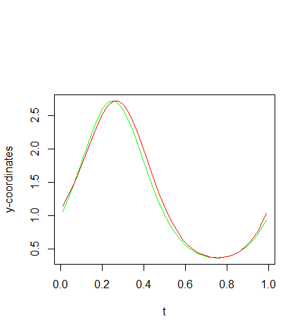
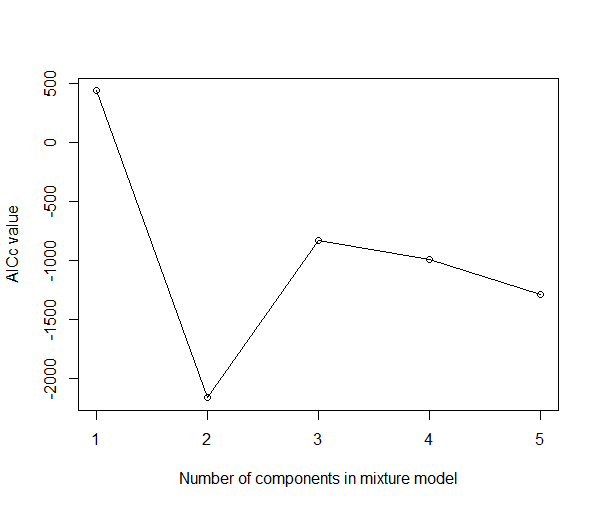
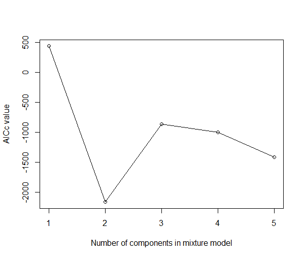
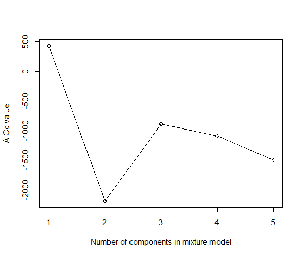
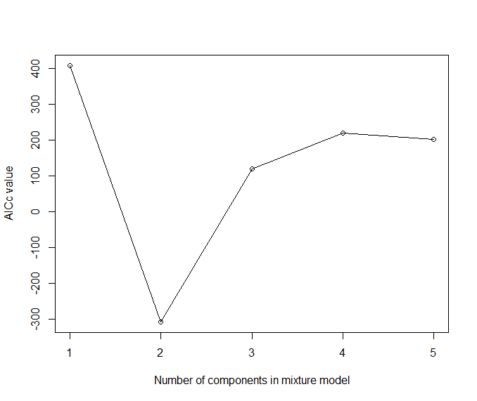
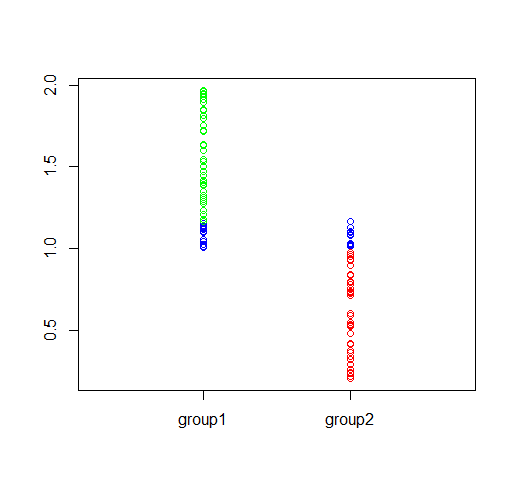
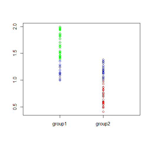
Four methods are applied to the simulated data D𝐷D in Scenario 1 with b1=0.12subscript𝑏10.12b_{1}=0.12, b2=0.8subscript𝑏20.8b_{2}=0.8, Scenario 2 with b1=0.10subscript𝑏10.10b_{1}=0.10, b2=0.8subscript𝑏20.8b_{2}=0.8, Scenario 3 with b1=0.08subscript𝑏10.08b_{1}=0.08, b2=0.8subscript𝑏20.8b_{2}=0.8 and Scenario 4 with b1=0.08subscript𝑏10.08b_{1}=0.08, b2=0.6subscript𝑏20.6b_{2}=0.6. Figure 2 and Figure 3 show the raw data depending on different b2subscript𝑏2b_{2} and b1subscript𝑏1b_{1} respectively. First of all, we apply the AICcsubscriptAIC𝑐\text{AIC}_{c} to choose the number of clusters. The results from Figure A.2 in Appendix 4 show that AICcsubscriptAIC𝑐\text{AIC}_{c} score reaches its minimum at 2 clusters. Table 1 summarizes the comparisons by average ARI and RI. Overall, both measures suggest that the proposed SRC outperform the other three methods in all scenarios because of the use of both functional and scalar data.
Refer to caption
(a) b2=0.8subscript𝑏20.8b_{2}=0.8
Refer to caption
(b) b2=0.6subscript𝑏20.6b_{2}=0.6
Figure 2: Observations of scalar variable in two cases. The ‘blue’ ones stand for those in the range of overlapping.
Refer to caption
Refer to caption
Refer to caption
(a) b1=0.08subscript𝑏10.08b_{1}=0.08
Refer to caption
Refer to caption
Refer to caption
(b) b1=0.10subscript𝑏10.10b_{1}=0.10
Refer to caption
Refer to caption
Refer to caption
(c) b1=0.12subscript𝑏10.12b_{1}=0.12
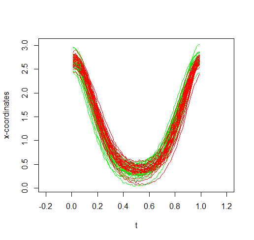
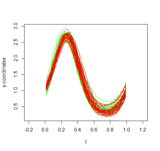
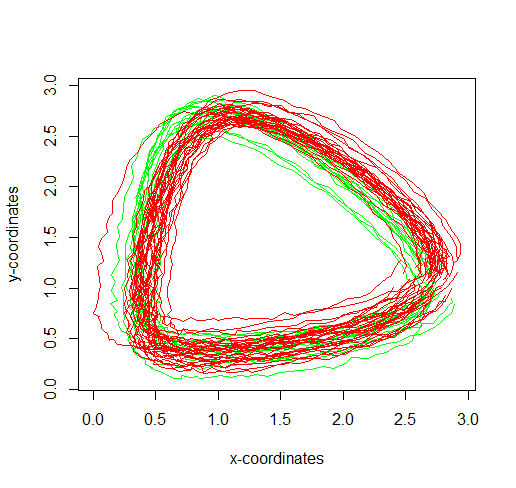
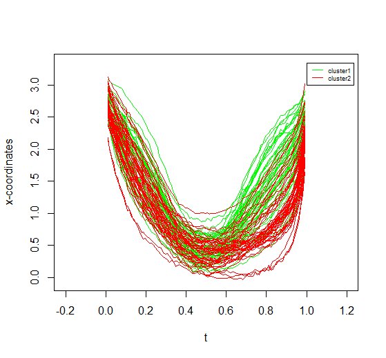
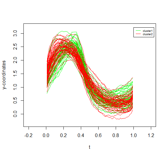
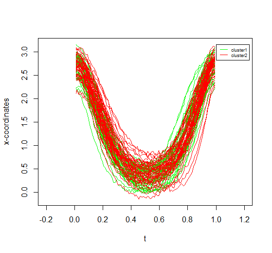
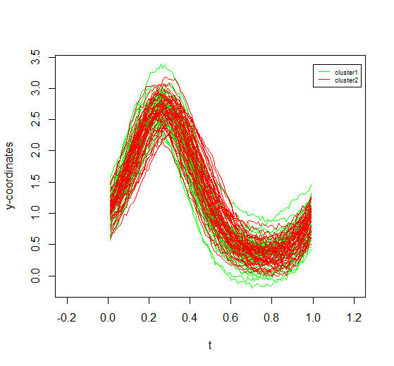
Figure 3: The raw 2D curves in one simulation run in three cases.

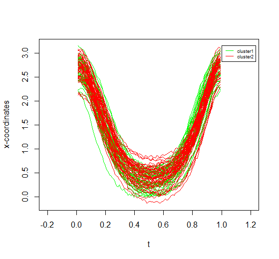
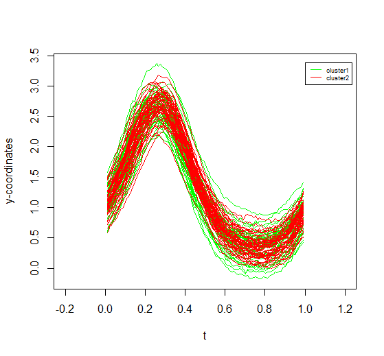
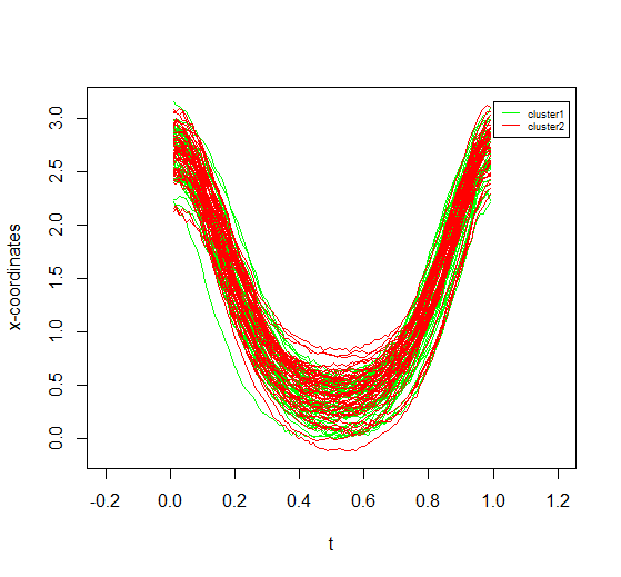
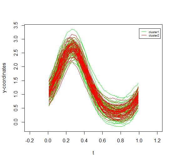
From Table 1, we note that all the four methods perform best in Scenario 1 compared to the other scenarios. In this scenario, both b1subscript𝑏1b_{1} and b2subscript𝑏2b_{2} take the largest values, indicating that overlapping of the functional data (Figure 3 (c)) and scalar data (Figure 2 (a)) are the smallest and both greatly contribute to distinguishing those two clusters. Though the other three methods, SRC-f, k-means-f and k-means-s based on either functional data or scalar data, also have good performance but not as good as SRC.

The first three scenarios share the same value of b2subscript𝑏2b_{2}, indicating that the degree of overlapping in two clusters for scalar data does not change (Figure 2 (a)). It causes the performance of k-means-s remaining the same. The overlapping in two clusters for functional data, however, gets smaller and smaller as the value of b1subscript𝑏1b_{1} decreases from Scenario 1 to Scenario 3. It leads to a sharp decline for the performance of SRC-f and k-means–f, both of which depend on functional data only, as opposed to a mild decrease of the performance of SRC, which is based on both scalar data and functional data.

The scenario 4 has the smallest b1subscript𝑏1b_{1} (Figure 3 (a)) and b2subscript𝑏2b_{2} (Figure 2 (b)) and it is quite difficult to carry out clustering just based on functional data or scalar data only. Consequently, the values of ARI for SRC-f, k-means-f and k-means-s are very small. But SRC still performs well and are much better than the others.

Other combinations with varying overlapping determined by b1subscript𝑏1b_{1} and b2subscript𝑏2b_{2} and with different sample sizes have also been examined. The results presented here are very typical.

Scenario 1 Scenario 2 Scenario 3 Scenario 4
RI ARI RI ARI RI ARI RI ARI
\hlineB4 SRC 0.980.98\mathbf{0.98} 0.960.96\mathbf{0.96} 0.950.95\mathbf{0.95} 0.900.90\mathbf{0.90} 0.910.91\mathbf{0.91} 0.820.82\mathbf{0.82} 0.800.80\mathbf{0.80} 0.610.61\mathbf{0.61}
SRC-f 0.90 0.80 0.75 0.49 0.62 0.25 0.62 0.25
k-means-f 0.91 0.83 0.76 0.53 0.64 0.29 0.64 0.29
k-means-s 0.81 0.62 0.81 0.62 0.81 0.62 0.69 0.37
Table 1: Comparison of average clustering results among four methods.

3.1.3 Recovery of curves and cluster patterns

To understand the underlying process better, it is necessary to use the optimally alignment to estimate the entire curve, so we estimate the aligned individual curves and reconstruct the cluster pattern using equation (9).

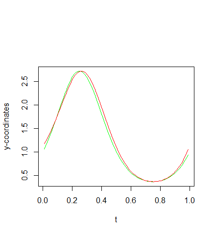
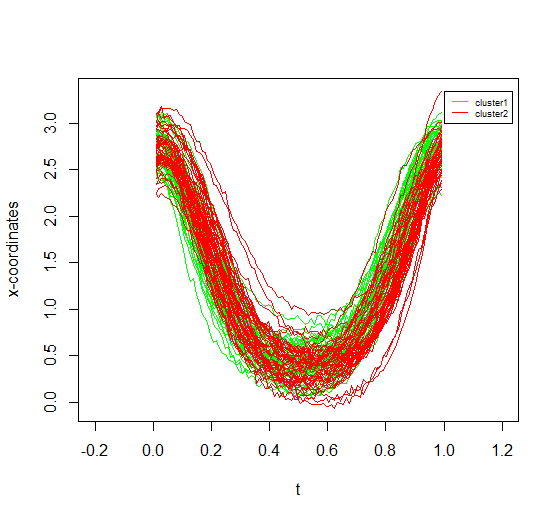
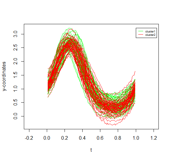
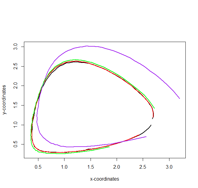
Figure A.3 in Appendix displays one simulation run of N=100𝑁100N=100, with N1=N2=50subscript𝑁1subscript𝑁250N_{1}=N_{2}=50 curves in each group. The top panel presents the original raw curves in the two clusters in two colors in two dimensions (x𝑥x-axis and y𝑦y-axis) for a new scenario with 4σw2=σr2=σ2=0.022,b1=0.15,b2=0.8formulae-sequence4superscriptsubscript𝜎𝑤2superscriptsubscript𝜎𝑟2superscript𝜎2superscript0.022formulae-sequencesubscript𝑏10.15subscript𝑏20.84\sigma_{w}^{2}=\sigma_{r}^{2}=\sigma^{2}=0.02^{2},b_{1}=0.15,b_{2}=0.8. The other panels respectively show the individual aligned curves resulting from SRC, SRC-f and k-means-f, with the value of RI (1, 0.63, 0.79) and the value of ARI (1, 0.26, 0.54) respectively. The SRC properly differentiates the two clusters (red and green) after curve alignment and performs better in recovering the cluster patterns.

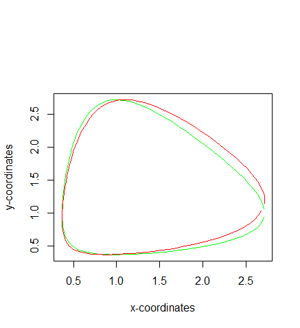
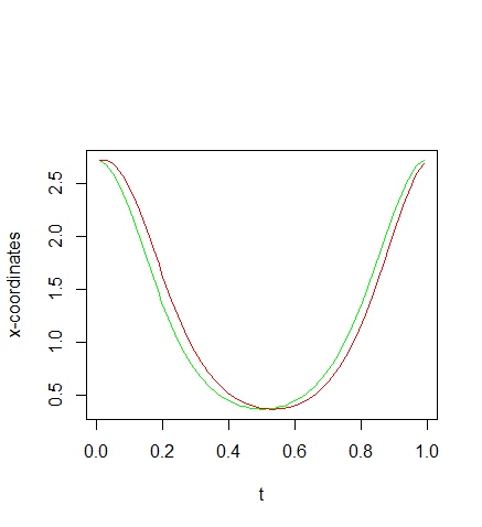
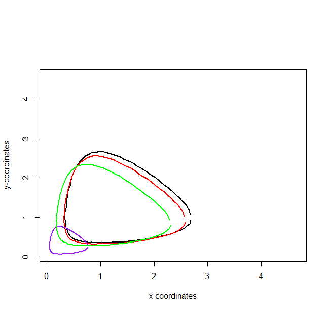
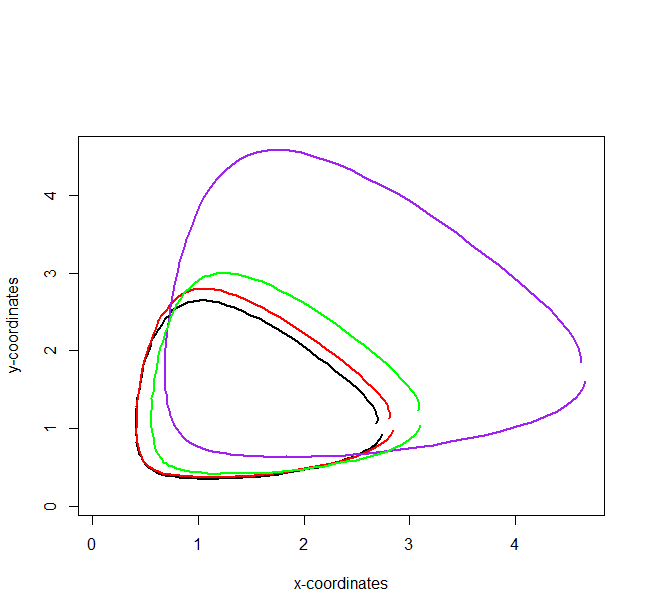
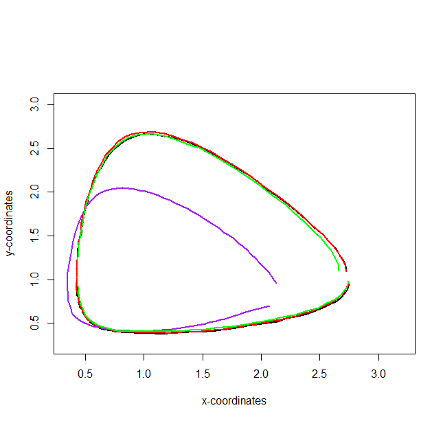
Figure 4 summarizes the result of clustering patterns. It shows the SRC method recovered the true pattens very well. As a measure of estimation error, we use the root average squared error (Gervini and Gasser,, 2004)

rase(𝝁^)=j=1m𝝁^(tj)𝝁(tj)2m,rase^𝝁superscriptsubscript𝑗1𝑚superscriptnorm^𝝁subscript𝑡𝑗𝝁subscript𝑡𝑗2𝑚\textit{rase}(\hat{\mbox{\boldmath${\mu}$}})=\sqrt{\frac{\sum_{j=1}^{m}||\hat{\mbox{\boldmath${\mu}$}}(t_{j})-\mbox{\boldmath${\mu}$}(t_{j})||^{2}}{m}},

where m𝑚m is the number of observation points, 𝝁(t)𝝁𝑡\mbox{\boldmath${\mu}$}(t) and 𝝁^(t)^𝝁𝑡\hat{\mbox{\boldmath${\mu}$}}(t) are the cross-sectional mean of 2D raw curves and of registered curves from the target method respectively. The values of rase are 2.9, 4.6 and 5.4 corresponding to three models SRC, SRC-f and k-means-f.
Refer to caption
(a) Cluster 1
Refer to caption
(b) Cluster 2
Figure 4: Mean functions for 2D curves in each cluster. black lines are true mean curves. red lines, purple lines and green lines stand for mean curves calculated from the results from SRC, SRC-f and k-means-f respectively.

One extreme scenario has been discussed in Appendix 5, providing further evidence of the good performance of the proposed SRC.

3.2 Real data analysis

The application to a real data is to cluster the normal people and the patients with stroke by studying their hyoid bone motion as well as the other scalar variables. Two groups, one for normal people and the other for patients, are included. Figure (1)(a) shows one frame from a X-ray video clip. The position of hyoid bone is tracked in each frame by a semi-automatic programme developed in Kim et al., (2017). The raw data before being preprocessed are shown in Figure (1)(b). There are 15 subjects in each group. The scalar variable we choose is the size of Pyriform Sinus Residue (see its position in Figure A.6). Regarding to those 2D curves, we firstly carry out the preprocessing procedures like multi-dimensional shift, scaling and rotation using the package of GPA. While modeling those curves, we assume the warping function be a smooth nonlinear deformation produced by an increasing spline and the random vector 𝒘kisubscript𝒘𝑘𝑖\bm{w}_{ki} be a Brownian bridge observed at discrete anchor points. B-spline basis functions are utilized for modeling the mean curves. The covariance function for the amplitude variance is the Matern covariance function.

We examine the performance of four methods SRC, SRC-f, k-means-f and k-means-s aforementioned. The values of AICc are shown in Figure A.7. It shows that the two-component mixture model has the smallest value. Table 2 shows the values of RI and ARI by comparing clustering results by the four methods with the clinic outcomes. We can see that the SRC method outperforms the other three. As a matter of fact, both SRC-f and k-means-f with value of RI equivalent to 0.5 fail in this real data example. It is similar to the extreme example in Appendix 5. More numerical results are provided in Appendix 6.

Model RI ARI
SRC 0.710.71\bm{0.71} 0.420.42\bm{0.42}
SRC-f 0.50 0.02
k-means-f 0.50 0.02
k-means-s 0.67 0.33
Table 2: Results of clustering by four methods for the real data

4 Conclusion

We have proposed a methodology for simultaneous registration and clustering, SRC, for multi-dimensional functional data which considers both the curves and scalar variables. This model captures the heterogeneity from the potential time warping for curves and scalar variables corresponding to each subject while carrying out the clustering in the meantime. It can be implemented with EM algorithm. Numerical examples show that it outperforms three other related methods, SRC-f, k-means-f and k-means-s. The results in Section 3.1.2 show that in most cases the inclusion of scalar variables can improve the performance of clustering in functional data analysis.

Generally, the registration for multi-dimensional functional data is much more complicated than one dimensional case. We use the pre-processing package GPA (Gower,, 1975) and a further registration via a simple warping function. The latter is one of the key parts in our model. This approach performs very well in the numerical examples presented in this article. Further research is however needed, for example, how to improve the iterative implementation for the complete registration, similar to the shape geodesic algorithm by the metric-based method proposed by Srivastava et al., 2011a . The inverse of warping function g𝑔g in model (1) can also be replaced with various types of other functions depending on types of data. The success of resolving registration problem often depends on the flexibility of choosing warping function.

Model selection is an interesting but difficult issue for a mixture model, especially for the models with complex forms. Kenneth and David, (2004) suggested AICc should be used unless NPL>40𝑁subscript𝑃𝐿40\frac{N}{P_{L}}>40 for the model with the large value of PLsubscript𝑃𝐿P_{L}. In our model, the number of parameters PLsubscript𝑃𝐿P_{L} is quite close to the number of subject N𝑁N. Thus, we use AICc. It works well for the examples discussed in the article. It is worth a further study under a general functional data analysis framework.

The results we obtained for the real data are encouraging although it is still in early stage. Research for this topic is carrying on. More features extracted from video clips along with other variables, both functional and scalar, are under investigation. Different types of models for data fitting, clustering/classification and prediction are being developed.

References

  • Bouveyron and Jacques, (2011) Bouveyron, C. and Jacques, J. (2011). Model-based clustering of time series in group-specific functional subspaces. Advances in Data Analysis and Classification, 5(4):281–300.
  • Cheng et al., (2016) Cheng, W., Dryden, L. L., and Huang, X. Z. (2016). Bayesian registration of functions and curves. Bayesian Analysis, 11(2):447–475.
  • Chiou and Li, (2007) Chiou, J. M. and Li, P. L. (2007). Functional clustering and identifying substructures of longitudinal data. J. R. Statist. Soc. B, 69(4):679–699.
  • Delaigle and Hall, (2010) Delaigle, A. and Hall, P. (2010). Defining probability density for a distribution of random functions. The Annals of Statistics, 38:1171–1193.
  • Ferraty and Vieu, (2006) Ferraty, F. and Vieu, P. (2006). Nonparametric functional data analysis. Springer Series in Statistics, Springer, New York.
  • Gervini and Gasser, (2004) Gervini, D. and Gasser, T. (2004). Self-modelling warping functions. J.R.Statist.Soc.B, 66(4):959–971.
  • Gower, (1975) Gower, J. C. (1975). Generalized procrustes analysis. Psychometrika, 40(1):33–51.
  • Green and Richardson, (2000) Green, P. J. and Richardson, S. (2000). Spatially corrrelated allocation models for count data.
  • Hartigan and Wong, (1978) Hartigan, J. A. and Wong, M. A. (1978). Algorithm as 1326: A k-means clustering algorithm. Applied Statistics, 28:100–108.
  • Hubert and Arabie, (1985) Hubert, L. and Arabie, P. (1985). Comparing partitions. J. Classif., 2:193–218.
  • Ieva et al., (2013) Ieva, F., Paganoni, A. M., Pigoli, D., and Vitelli, V. (2013). Multivariate functional clustering for the analysis of ecg curves morphology. Journal of the Royal Statistical Society. Series C, 62(3):401–418.
  • James and Sugar, (2003) James, G. M. and Sugar, C. A. (2003). Clustering for sparsely sampled functional data. Journal of the American Statistical Association, 98(462):397–408.
  • Kenneth and David, (2004) Kenneth, P. B. and David, R. A. (2004). Understanding aic and bic in model selection. Sociological Methods Research, 33:261–304.
  • Kim et al., (2017) Kim, W.-S., Zeng, P., Shi, J. Q., Lee, Y., and Paik, N.-J. (2017). Automatic tracking of hyoid bone motion from videofluoroscopic swallowing study with automatic smoothing and segmentation. PLOS ONE, page (to appear).
  • Liu and Yang, (2009) Liu, X. and Yang, M. C. K. (2009). Simultaneous curve registration and clustering for functional data. Computational Statistics and Data Analysis, 53:1361–1376.
  • Lloyd, (1982) Lloyd, S. P. (1982). Least squares quantization in pcm. IEEE Transactions on Information Theory, 28(2):129–137.
  • MacQueen, (1967) MacQueen, J. B. (1967). Some methods for classification and analysis of multivariate observations. Proceedings of 5th Berkeley Symposium on Mathematical Statistics and Probability. University of California Press., pages 281–297.
  • Marron et al., (2015) Marron, J., Ramsay, J. O., Sangalli, L. M., and Srivastava, A. (2015). Functional data analysis of amplitude and phase variation. Statistical Science, 30(4):468–484.
  • Raket, (2016) Raket, L. L. (2016). pavpop version 0.10. Available at http://github.com/larslau/pavpop/.
  • Raket et al., (2016) Raket, L. L., Grimme, B., Schoner, G., Igel, C., and Markussen, B. (2016). Separating timing, movement conditions and individual differences in the analysis of human movement. PLoS Comput Biol, 12(9).
  • Ramsay and Silverman, (2005) Ramsay, J. O. and Silverman, B. W. (2005). Functional Data Analysis. Springer-Verlag New York, USA.
  • Rand, (1971) Rand, W. M. (1971). Objective criteria for the evaluation of clustering methods. J. Am. Stat. Assoc., 66:846–850.
  • Sam et al., (2011) Sam, A., Chamroukhi, F., Govaert, G., and Aknin, P. (2011). Model-based clustering and segmentation of time series with changes in regime. Advances in Data Analysis and Classification, 5(4):301–322.
  • Sangalli et al., (2009) Sangalli, L. M., Secchi, P., Vantini, S., and Veneziani, A. (2009). A case study in exploratory functional data analysis: geometrical features of the internal carotid artery. J.Amer.Statist.Assoc., 104:37–48.
  • Sangalli et al., (2010) Sangalli, L. M., Secchi, P., Vantini, S., and Vitelli, V. (2010). k-mean alignment for curve clustering. Computational Statistics & Data Analysis, 54(5):1219–1233.
  • Shi and Choi, (2011) Shi, J. Q. and Choi, T. (2011). Gaussian Process Regression Analysis for Functional Data. CRC Press Taylor & Francis Group.
  • Shi et al., (2005) Shi, J. Q., Murray-Smith, R., and Titterington, D. M. (2005). Hierarchical gaussian process mixtures for regression. Statistics and Computing, 15:31–41.
  • Shi and Wang, (2008) Shi, J. Q. and Wang, B. (2008). Curve prediction and clustering with mixtures of gaussian process functional regression models. Stat Comput, 18(3):267–283.
  • Shi et al., (2012) Shi, J. Q., Wang, B., Will, E. J., and West, R. M. (2012). Mixed-effect gaussian process functional regression models with application to dose-response curve prediction. Statist. Med., 31:3165–3177.
  • (30) Srivastava, A., Klassen, E., Joshi, S. H., and Jermyn, I. H. (2011a). Shape analysis of elastic curves in euclidean spaces. IEEE Trans. Pattern.Anal.Mach.Intell, 33(7):1415–1428.
  • (31) Srivastava, A., Wu, W., Kurtek, S., Klassen, E., and Marron, J. S. (2011b). Registration of functional data using the fisher-rao metric. Preprint. Available at arXiv:1103.3817v2.
  • Sugiura and Nariaki, (1978) Sugiura and Nariaki (1978). Further analysis of the data by akaike’s information criterion and the finite corrections. Communications in Statistics, Theory and Methods, A7:13–26.
  • Tang and Müller, (1998) Tang, R. and Müller, H. G. (1998). Pairwise curve synchronization for functional data. Biometricka, 95(4):875–889.
  • Tarpey and Kinateder, (2003) Tarpey, T. and Kinateder, K. J. (2003). Clustering functional data. Journal of Classification, 20(1):93–114.
  • Tokushige et al., (2007) Tokushige, S., Yadohisa, H., and Inada, K. (2007). Crisp and fuzzy k-means clustering algorithms for multivariate functional data. Computational Statistics, 22:1–16.

Appendices

Appendix 1 Derivation of Mkisubscript𝑀𝑘𝑖M_{ki}

Using Bayes’ theorem, the posterior distribution with respect to 𝐳𝐳\mathbf{z} has the form

p(𝒛|𝒙,𝜽,𝜷)i=1Nk=1Kπkizkip(𝒙i|𝜽ki)zki.proportional-to𝑝conditional𝒛𝒙𝜽𝜷superscriptsubscriptproduct𝑖1𝑁superscriptsubscriptproduct𝑘1𝐾superscriptsubscript𝜋𝑘𝑖subscript𝑧𝑘𝑖𝑝superscriptconditionalsubscript𝒙𝑖subscript𝜽𝑘𝑖subscript𝑧𝑘𝑖p(\mbox{\boldmath${z}$}|\mbox{\boldmath${x}$},\mbox{\boldmath${\theta}$},\mbox{\boldmath${\beta}$})\propto\prod_{i=1}^{N}\prod_{k=1}^{K}\pi_{ki}^{z_{ki}}p(\mbox{\boldmath${x}$}_{i}|\mbox{\boldmath${\theta}$}_{ki})^{z_{ki}}.

By factorizing it over i𝑖i, it is clear that the {𝒛i,i=1,,N}formulae-sequencesubscript𝒛𝑖𝑖1𝑁\{\mbox{\boldmath${z}$}_{i},i=1,\dots,N\} are independent under the posterior distribution. Hence,

E(zki|𝒙,𝜽,𝜷)=E(zki|𝒙i,𝜽,𝜷)=p(zki=1|𝒙i,𝜽,𝜷)=p(zki=1|𝜷)p(𝒙i|zki=1,𝜽)p(𝒙i|𝜽,𝜷)=πkip(𝒙i|𝜽ki)p(𝒙i|𝜽,𝜷).𝐸conditionalsubscript𝑧𝑘𝑖𝒙𝜽𝜷𝐸conditionalsubscript𝑧𝑘𝑖subscript𝒙𝑖𝜽𝜷𝑝subscript𝑧𝑘𝑖conditional1subscript𝒙𝑖𝜽𝜷𝑝subscript𝑧𝑘𝑖conditional1𝜷𝑝conditionalsubscript𝒙𝑖subscript𝑧𝑘𝑖1𝜽𝑝conditionalsubscript𝒙𝑖𝜽𝜷subscript𝜋𝑘𝑖𝑝conditionalsubscript𝒙𝑖subscript𝜽𝑘𝑖𝑝conditionalsubscript𝒙𝑖𝜽𝜷\begin{split}E(z_{ki}|\mbox{\boldmath${x}$},\mbox{\boldmath${\theta}$},\mbox{\boldmath${\beta}$})&=E(z_{ki}|\mbox{\boldmath${x}$}_{i},\mbox{\boldmath${\theta}$},\mbox{\boldmath${\beta}$})\\ &=p(z_{ki}=1|\mbox{\boldmath${x}$}_{i},\mbox{\boldmath${\theta}$},\mbox{\boldmath${\beta}$})\\ &=\frac{p(z_{ki}=1|\mbox{\boldmath${\beta}$})p(\mbox{\boldmath${x}$}_{i}|z_{ki}=1,\mbox{\boldmath${\theta}$})}{p(\mbox{\boldmath${x}$}_{i}|\mbox{\boldmath${\theta}$},\mbox{\boldmath${\beta}$})}\\ &=\frac{\pi_{ki}p(\mbox{\boldmath${x}$}_{i}|\mbox{\boldmath${\theta}$}_{ki})}{p(\mbox{\boldmath${x}$}_{i}|\mbox{\boldmath${\theta}$},\mbox{\boldmath${\beta}$})}.\end{split} (A.1)

We know that

p(𝒙i|𝜽,𝜷)=𝒛ip(𝒛i|𝜷)p(𝒙i|𝒛i,𝜽,𝜷)=zkik=1K(p(zki=1|𝜷)p(𝒙i|zki=1,𝜽))zki=j=1Kπjip(𝒙i|𝜽ji).𝑝conditionalsubscript𝒙𝑖𝜽𝜷subscriptsubscript𝒛𝑖𝑝conditionalsubscript𝒛𝑖𝜷𝑝conditionalsubscript𝒙𝑖subscript𝒛𝑖𝜽𝜷subscriptsubscript𝑧𝑘𝑖superscriptsubscriptproduct𝑘1𝐾superscript𝑝subscript𝑧𝑘𝑖conditional1𝜷𝑝conditionalsubscript𝒙𝑖subscript𝑧𝑘𝑖1𝜽subscript𝑧𝑘𝑖superscriptsubscript𝑗1𝐾subscript𝜋𝑗𝑖𝑝conditionalsubscript𝒙𝑖subscript𝜽𝑗𝑖\begin{split}p(\mbox{\boldmath${x}$}_{i}|\mbox{\boldmath${\theta}$},\mbox{\boldmath${\beta}$})&=\sum_{\mbox{\boldmath${z}$}_{i}}p(\mbox{\boldmath${z}$}_{i}|\mbox{\boldmath${\beta}$})p(\mbox{\boldmath${x}$}_{i}|\mbox{\boldmath${z}$}_{i},\mbox{\boldmath${\theta}$},\mbox{\boldmath${\beta}$})\\ &=\sum_{z_{ki}}\prod_{k=1}^{K}\big{(}p(z_{ki}=1|\mbox{\boldmath${\beta}$})p(\mbox{\boldmath${x}$}_{i}|z_{ki}=1,\mbox{\boldmath${\theta}$})\big{)}^{z_{ki}}\\ &=\sum_{j=1}^{K}\pi_{ji}p(\mbox{\boldmath${x}$}_{i}|\mbox{\boldmath${\theta}$}_{ji}).\end{split} (A.2)

Thus,

E(zki|𝒙,𝜽,𝜷)=πkip(𝒙i|𝜽ki)j=1Kπjip(𝒙i|𝜽ji).𝐸conditionalsubscript𝑧𝑘𝑖𝒙𝜽𝜷subscript𝜋𝑘𝑖𝑝conditionalsubscript𝒙𝑖subscript𝜽𝑘𝑖superscriptsubscript𝑗1𝐾subscript𝜋𝑗𝑖𝑝conditionalsubscript𝒙𝑖subscript𝜽𝑗𝑖E(z_{ki}|\mbox{\boldmath${x}$},\mbox{\boldmath${\theta}$},\mbox{\boldmath${\beta}$})=\frac{\pi_{ki}p(\mbox{\boldmath${x}$}_{i}|\mbox{\boldmath${\theta}$}_{ki})}{\sum_{j=1}^{K}\pi_{ji}p(\mbox{\boldmath${x}$}_{i}|\mbox{\boldmath${\theta}$}_{ji})}.

Appendix 2 Derivation of the linearized model

At the linearized level, we do the first-order Taylor approximation of model (3) in Section 2.2 in the random warp 𝒘kisubscript𝒘𝑘𝑖\mbox{\boldmath${w}$}_{ki}. We reconsider gki(t)subscript𝑔𝑘𝑖𝑡g_{ki}(t) as a function with respect to 𝒘ksubscript𝒘𝑘\mbox{\boldmath${w}$}_{k} + 𝒘kisubscript𝒘𝑘𝑖\mbox{\boldmath${w}$}_{ki}. Thus, the linearization can be carried out around the estimate of 𝒘ksubscript𝒘𝑘\mbox{\boldmath${w}$}_{k} plus 𝒘ki0subscriptsuperscript𝒘0𝑘𝑖\mbox{\boldmath${w}$}^{0}_{ki} obtained from the previous step. This results in a linear mixed-effects model as follows:

𝒙ai|zki=1𝒙ai|zki=1,𝒘ki=𝒘ki0+𝒘ki(𝒙ai|zki=1)|𝒘ki=𝒘ki0(𝒘ki𝒘ki0)evaluated-atsubscript𝒙𝑎𝑖subscript𝑧𝑘𝑖1evaluated-atsubscript𝒙𝑎𝑖subscript𝑧𝑘𝑖1subscript𝒘𝑘𝑖subscriptsuperscript𝒘0𝑘𝑖evaluated-atsubscriptsubscript𝒘𝑘𝑖evaluated-atsubscript𝒙𝑎𝑖subscript𝑧𝑘𝑖1subscript𝒘𝑘𝑖subscriptsuperscript𝒘0𝑘𝑖subscript𝒘𝑘𝑖subscriptsuperscript𝒘0𝑘𝑖\mbox{\boldmath${x}$}_{ai}|_{z_{ki=1}}\approx\mbox{\boldmath${x}$}_{ai}|_{z_{ki=1},\mbox{\boldmath${w}$}_{ki}=\mbox{\boldmath${w}$}^{0}_{ki}}+\nabla_{\mbox{\boldmath${w}$}_{ki}}({\mbox{\boldmath${x}$}_{ai}|_{z_{ki=1}}})|_{\mbox{\boldmath${w}$}_{ki}=\mbox{\boldmath${w}$}^{0}_{ki}}(\mbox{\boldmath${w}$}_{ki}-\mbox{\boldmath${w}$}^{0}_{ki})

where

𝒙ai|zki=1,𝒘ki=𝒘ki0evaluated-atsubscript𝒙𝑎𝑖subscript𝑧𝑘𝑖1subscript𝒘𝑘𝑖subscriptsuperscript𝒘0𝑘𝑖\displaystyle\mbox{\boldmath${x}$}_{ai}|_{z_{ki=1},\mbox{\boldmath${w}$}_{ki}=\mbox{\boldmath${w}$}^{0}_{ki}} =𝝉𝒂𝒌(gki)|𝒘ki=𝒘ki0+𝒓aki+ϵabsentevaluated-atsubscript𝝉𝒂𝒌subscript𝑔𝑘𝑖subscript𝒘𝑘𝑖subscriptsuperscript𝒘0𝑘𝑖subscript𝒓𝑎𝑘𝑖bold-italic-ϵ\displaystyle=\mbox{\boldmath${\tau_{ak}}$}(g_{ki})|_{\mbox{\boldmath${w}$}_{ki}=\mbox{\boldmath${w}$}^{0}_{ki}}+\mbox{\boldmath${r}$}_{aki}+\mbox{\boldmath${\epsilon}$}
=𝚿ki|gki=gki0𝒅ak+𝒓aki+ϵabsentevaluated-atsubscript𝚿𝑘𝑖subscript𝑔𝑘𝑖superscriptsubscript𝑔𝑘𝑖0subscript𝒅𝑎𝑘subscript𝒓𝑎𝑘𝑖bold-italic-ϵ\displaystyle=\mbox{\boldmath${\Psi}$}_{ki}|_{g_{ki}=g_{ki}^{0}}\mbox{\boldmath${d}$}_{ak}+\mbox{\boldmath${r}$}_{aki}+\mbox{\boldmath${\epsilon}$}

and according to the chain rule,

𝒘ki(𝒙ai|zki=1)|𝒘ki=𝒘ki0evaluated-atsubscriptsubscript𝒘𝑘𝑖evaluated-atsubscript𝒙𝑎𝑖subscript𝑧𝑘𝑖1subscript𝒘𝑘𝑖subscriptsuperscript𝒘0𝑘𝑖\displaystyle\nabla_{\mbox{\boldmath${w}$}_{ki}}({\mbox{\boldmath${x}$}_{ai}|_{z_{ki=1}}})|_{\mbox{\boldmath${w}$}_{ki}=\mbox{\boldmath${w}$}^{0}_{ki}} ={𝒙ai|zki=1,t=tjgki(𝒘ki(gki(tj)))|𝒘ki=𝒘ki0}jabsentsubscriptevaluated-atevaluated-atsubscript𝒙𝑎𝑖subscript𝑧𝑘𝑖1𝑡subscript𝑡𝑗subscript𝑔𝑘𝑖superscriptsubscriptsubscript𝒘𝑘𝑖subscript𝑔𝑘𝑖subscript𝑡𝑗subscript𝒘𝑘𝑖subscriptsuperscript𝒘0𝑘𝑖𝑗\displaystyle=\Bigg{\{}\frac{\partial{\mbox{\boldmath${x}$}_{ai}|_{z_{ki=1},t=t_{j}}}}{\partial{g_{ki}}}\bigg{(}\nabla_{\mbox{\boldmath${w}$}_{ki}}\big{(}g_{ki}(t_{j})\big{)}\bigg{)}^{\intercal}\Big{|}_{\mbox{\boldmath${w}$}_{ki}=\mbox{\boldmath${w}$}^{0}_{ki}}\Bigg{\}}_{j}
={(τak(gki(tj)))gki|gki=gki0(𝒘ki(gki(tj)))|𝒘ki=𝒘ki0}jni×nw.absentsubscriptevaluated-atevaluated-atsubscript𝜏𝑎𝑘subscript𝑔𝑘𝑖subscript𝑡𝑗subscript𝑔𝑘𝑖subscript𝑔𝑘𝑖superscriptsubscript𝑔𝑘𝑖0superscriptsubscriptsubscript𝒘𝑘𝑖subscript𝑔𝑘𝑖subscript𝑡𝑗subscript𝒘𝑘𝑖superscriptsubscript𝒘𝑘𝑖0𝑗superscriptsubscript𝑛𝑖subscript𝑛𝑤\displaystyle=\bigg{\{}\frac{\partial\Big{(}\tau_{ak}\big{(}g_{ki}(t_{j})\big{)}\Big{)}}{\partial{g_{ki}}}\Big{|}_{g_{ki}=g_{ki}^{0}}\Big{(}\nabla_{\mbox{\boldmath${w}$}_{ki}}\big{(}g_{ki}(t_{j})\big{)}\Big{)}^{\intercal}\Big{|}_{\mbox{\boldmath${w}$}_{ki}=\mbox{\boldmath${w}$}_{ki}^{0}}\bigg{\}}_{j}\in\mathds{R}^{n_{i}\times n_{w}}.

In practical, we use finite difference for calculating the derivative of gki(t)subscript𝑔𝑘𝑖𝑡g_{ki}(t) with respect to 𝒘kisubscript𝒘𝑘𝑖\mbox{\boldmath${w}$}_{ki}.

Appendix 3 Implementation of functional k𝑘k-means

We just use d=||||2d=||\cdot||^{2} for the purpose of simplicity and convenience. The iterative procedures are as follows:

  1. 1.

    Choose the initial values for the zkisubscript𝑧𝑘𝑖z_{ki}. We can use any clustering method for scalar variables {𝜷i}subscript𝜷𝑖\{\mbox{\boldmath${\beta}$}_{i}\} corresponding to the functional variables {𝒙i}subscript𝒙𝑖\{\mbox{\boldmath${x}$}_{i}\}.

  2. 2.

    Fix zkisubscript𝑧𝑘𝑖z_{ki} and minimize F𝐹F with respect to the 𝝉ak(gki)subscript𝝉𝑎𝑘subscript𝑔𝑘𝑖\mbox{\boldmath${\tau}$}_{ak}(g_{ki}). In this phase, minimizing F𝐹F is equivalent to maximizing

    k=1Ki=1Nzki(a=12(logp(𝒙ai|𝜽aki)))superscriptsubscript𝑘1𝐾superscriptsubscript𝑖1𝑁subscript𝑧𝑘𝑖superscriptsubscript𝑎12log𝑝conditionalsubscript𝒙𝑎𝑖subscript𝜽𝑎𝑘𝑖\sum_{k=1}^{K}\sum_{i=1}^{N}z_{ki}\bigg{(}\sum_{a=1}^{2}\big{(}\text{log}p(\mbox{\boldmath${x}$}_{ai}|\mbox{\boldmath${\theta}$}_{aki})\big{)}\bigg{)}

    with the assumption that the covariance matrix of 𝒙aisubscript𝒙𝑎𝑖\mbox{\boldmath${x}$}_{ai} are the same over all the subjects. The detailed estimation of {𝜽aki}subscript𝜽𝑎𝑘𝑖\{\mbox{\boldmath${\theta}$}_{aki}\} have been mentioned before and the 𝝉ak(gki)subscript𝝉𝑎𝑘subscript𝑔𝑘𝑖\mbox{\boldmath${\tau}$}_{ak}(g_{ki}) can be obtained straightforwardly.

  3. 3.

    Fix 𝝉ak(gki)subscript𝝉𝑎𝑘subscript𝑔𝑘𝑖\mbox{\boldmath${\tau}$}_{ak}(g_{ki}) and minimize F𝐹F with respect to zkisubscript𝑧𝑘𝑖z_{ki}. Since the term F𝐹F in (10) involving different i𝑖i are independent, we can optimize F𝐹F for each i𝑖i separately by choosing zkisubscript𝑧𝑘𝑖z_{ki} as follows

    zki={1,ifk=argminj(𝒙i𝝉j(gji))2;0,otherwise.subscript𝑧𝑘𝑖cases1if𝑘subscript𝑗superscriptnormsubscript𝒙𝑖subscript𝝉𝑗subscript𝑔𝑗𝑖2missing-subexpression0otherwisemissing-subexpressionz_{ki}=\left\{\begin{array}[]{ll}1,\hskip 5.69054pt\text{if}\hskip 5.69054ptk=\arg\!\min_{j}||\big{(}\mbox{\boldmath${x}$}_{i}-\mbox{\boldmath${\tau}$}_{j}(g_{ji})\big{)}||^{2};\\ 0,\hskip 5.69054pt\text{otherwise}.\end{array}\right.
  4. 4.

    Repeat Step 2 and Step 3 until convergence.

Appendix 4 Extra numerical results in simulation study

Figures A.1 to A.3 provide extra numerical results for the simulated examples discussed in Section 3.1.

An extra example is given below.

Appendix 5 A simulation example in an extreme scenario

It is not uncommon that sometimes the functional variables provide little information so that it fails to implement the clustering just based on those curves. However, the addition of scalar variables can make the clustering possible. We simulate a run of N=100𝑁100N=100 (sample size), with 4σw2=σr2=σ2=0.022,b1=0.05,b2=0.8formulae-sequence4superscriptsubscript𝜎𝑤2superscriptsubscript𝜎𝑟2superscript𝜎2superscript0.022formulae-sequencesubscript𝑏10.05subscript𝑏20.84\sigma_{w}^{2}=\sigma_{r}^{2}=\sigma^{2}=0.02^{2},b_{1}=0.05,b_{2}=0.8, and N1=N2=50subscript𝑁1subscript𝑁250N_{1}=N_{2}=50 curves in each group. Figure A.4 displays the individual aligned curves resulting from three methods, from which no discernible clusters are visiable. The RI and ARI for SRC, SRC-f and k-means-f are, however, markedly different with the values of (0.82,0.50,0.50)0.820.500.50(0.82,0.50,0.50) and (0.64,0,0)0.6400(0.64,0,0) respectively. Figure A.5 summarizes the mean functions of two clusters by three methods. Their values of rase are 1.1, 18.3 and 4.3 respectively. Those results show that the use of SRC leads to meaningful findings but the other twos are equivalent to random guess.

Appendix 6 Extra numerical results in real data analysis

Figures A.6 to A.9 provide extra numerical results for the real data example discussed in Section 3.2.

Figure A.9 shows the clustering results by SRC along with the registering effect, which are quite close to the true data shown in Figure A.8.
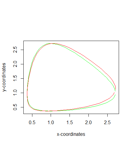
Refer to caption
Refer to caption
Refer to caption
(a) b1=0.08subscript𝑏10.08b_{1}=0.08
Refer to caption
Refer to caption
Refer to caption
(b) b1=0.10subscript𝑏10.10b_{1}=0.10
Refer to caption
Refer to caption
Refer to caption
(c) b1=0.12subscript𝑏10.12b_{1}=0.12
Figure A.1: True mean curves 𝝁1(t)subscript𝝁1𝑡\bm{\mu}_{1}(t) (indicated by green lines) and 𝝁2(t)subscript𝝁2𝑡\bm{\mu}_{2}(t) (indicated by red lines) of group 1 and group 2 with b1=0.08,0.10,0.12subscript𝑏10.080.100.12b_{1}=0.08,0.10,0.12.
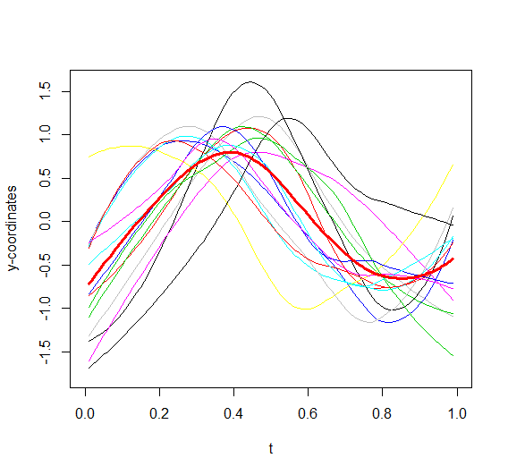
Refer to caption
(a) Scenario 1
Refer to caption
(b) Scenario 2
Refer to caption
(c) Scenario 3
Refer to caption
(d) Scenario 4
Figure A.2: The value of AICc calculated from one replication in each scenario for the method SRC.
Refer to caption
(a) Original 𝒙1(t)subscript𝒙1𝑡\mbox{\boldmath${x}$}_{1}(t)
Refer to caption
(b) Original 𝒙2(t)subscript𝒙2𝑡\mbox{\boldmath${x}$}_{2}(t)
Refer to caption
(c) SRC, aligned 𝒙1(t)subscript𝒙1𝑡\mbox{\boldmath${x}$}_{1}(t)
Refer to caption
(d) SRC, aligned 𝒙2(t)subscript𝒙2𝑡\mbox{\boldmath${x}$}_{2}(t)
Refer to caption
(e) SRC-f, aligned 𝒙1(t)subscript𝒙1𝑡\mbox{\boldmath${x}$}_{1}(t)
Refer to caption
(f) SRC-f, aligned 𝒙2(t)subscript𝒙2𝑡\mbox{\boldmath${x}$}_{2}(t)
Refer to caption
(g) k-means-f, aligned 𝒙1(t)subscript𝒙1𝑡\mbox{\boldmath${x}$}_{1}(t)
Refer to caption
(h) k-means-f, aligned 𝒙2(t)subscript𝒙2𝑡\mbox{\boldmath${x}$}_{2}(t)
Figure A.3: (a) and (b) are simulated 2D curves of two groups (green and red). (c)-(h) are aligned individual cruves by SRC, SRC-f and k-means-f.
Refer to caption
(a) Original 𝒙1(t)subscript𝒙1𝑡\mbox{\boldmath${x}$}_{1}(t)
Refer to caption
(b) Original 𝒙2(t)subscript𝒙2𝑡\mbox{\boldmath${x}$}_{2}(t)
Refer to caption
(c) SRC, aligned 𝒙1(t)subscript𝒙1𝑡\mbox{\boldmath${x}$}_{1}(t)
Refer to caption
(d) SRC, aligned 𝒙2(t)subscript𝒙2𝑡\mbox{\boldmath${x}$}_{2}(t)
Refer to caption
(e) SRC-f, aligned 𝒙1(t)subscript𝒙1𝑡\mbox{\boldmath${x}$}_{1}(t)
Refer to caption
(f) SRC-f, aligned 𝒙2(t)subscript𝒙2𝑡\mbox{\boldmath${x}$}_{2}(t)
Refer to caption
(g) k-means-f, aligned 𝒙1(t)subscript𝒙1𝑡\mbox{\boldmath${x}$}_{1}(t)
Refer to caption
(h) k-means-f, aligned 𝒙2(t)subscript𝒙2𝑡\mbox{\boldmath${x}$}_{2}(t)
Figure A.4: (a) and (b) are simulated 2D curves of two groups (green and red). (c)-(h) are aligned individual cruves by SRC, SRC-f and k-means-f.
Refer to caption
(a) Cluster 1
Refer to caption
(b) Cluster 2
Figure A.5: Mean functions for 2D curves from two clusters. The black lines are true mean functions. The red lines, purple lines and green lines are respectively corresponding to results obtained from the model SRC, SRC-f and k-means-f.
Refer to caption
Figure A.6: Highlight of Pyriform Sinus Residue, covered by the red circle
Refer to caption
Figure A.7: The values of AICc for SRC𝑆𝑅𝐶SRC
Refer to caption
Refer to caption
Refer to caption
(a) Curves from 15 normal people
Refer to caption
Refer to caption
Refer to caption
(b) Curves from 15 abnormal people
Figure A.8: Curves of hyoid bone motion for two true groups, where the bold curves in green (upper panel) and in red (lower panel) are the average mean curve for each group
Refer to caption
Refer to caption
Refer to caption
(a) Cluster 1 with 16 people
Refer to caption
Refer to caption
Refer to caption
(b) Cluster 2 with 14 people
Figure A.9: Curves of hyoid bone motion for two groups clustered by SRC, where the bold curves in green (upper panel) and in red (lower panel) are the average mean curve for each group