Electric Dipole Moment Results from lattice QCD

Abstract

We utilize the gradient flow to define and calculate electric dipole moments induced by the strong QCD $\theta$-term and the dimension-6 Weinberg operator. The gradient flow is a promising tool to simplify the renormalization pattern of local operators. The results of the nucleon electric dipole moments are calculated on PACS-CS gauge fields (available from the ILDG) using $N_{f}=2+1$, of discrete size $32^{3}\times 64$ and spacing $a\simeq 0.09$ fm. These gauge fields use a renormalization-group improved gauge action and a non-perturbatively $O(a)$ improved clover quark action at $\beta=1.90$, with $c_{SW}=1.715$. The calculation is performed at pion masses of $m_{\pi}\simeq 411,701$ MeV.

1 Introduction

The study of the electric dipole moment of the neutron and proton (nEDM & pEDM) provides us a tool for understanding how different sources of CP violation manifest in hadronic systems. Experimentally, the total nEDM has been bounded by $|d_{n}|<3.0\times 10^{-13}$ e fm Olive:2016xmw . A weaker bound of $|d_{p}|<2.0\times 10^{-12}$ e fm Graner:2016ses has been achieved indirectly from the limit of the Hg EDM, in this way overcoming the difficulties of observing an EDM of a charged system.

The Standard Model (SM) contains the “$\theta$-term” which can induce an EDM in the neutron and proton. At the same time, Beyond the Standard Model (BSM) physics can also provide contributions to EDMs. At hadronic energies these can be parametrized by effective higher-dimensional operators that violate CP.

Due to recent advancements in computational power and theoretical developments, lattice QCD is fast approaching the precision needed to calculate the EDM of the neutron and proton Alexandrou:2015spa ; Guo:2015tla . The key feature when providing this ab-initio calculation from lattice QCD, is that the individual contributions from the $\theta$-term and all the BSM operators can be calculated individually. These calculations, combined with future experimental results, can provide unique constraints for the different types of BSM CP violations responsible for a non-vanishing EDM.

In this work, we analyze the nEDM and pEDM induced by the $\theta$ and Weinberg terms individually. We use the gradient flow to define the $\theta$-term and the Weinberg operator on the lattice. For the $\theta$-term, the use of gradient flow circumvents the problems associated with renormalization. For the Weinberg operator it provides a powerful method to connect the divergent-free definition of the corresponding correlation functions at non-vanishing flow time with the physical matrix element.

2 Theory

The QCD Lagrangian in Euclidean space without strong CP violation, has the form

$$\mathcal{L}_{QCD}=\frac{1}{4}G_{\mu\nu}^{a}G_{\mu\nu}^{a}+\sum_{q=u,d,s}\overline{\psi}_{q}\left(\gamma_{\mu}D_{\mu}+m_{q}\right)\psi_{q}\,,$$ (1)

where $G_{\mu\nu}^{a}$ denotes the gluonic field strength, $\psi_{u,d,s}$ denote the up, down, and strange quarks, $\gamma_{\mu}D_{\mu}$ the gauge-covariant derivative, and $m_{q}$ the fermion quark masses . We consider two CP-violating terms in this contribution. The first is the “$\theta$-term” proportional to the topological charge density $q(x)$

$$-i\theta q(x)\equiv-i\theta\frac{1}{32\pi^{2}}\epsilon_{\mu\nu\rho\sigma}\mathrm{Tr}\left[G_{\mu\nu}(x)G_{\rho\sigma}(x)\right],$$

and the second is the Weinberg operator Weinberg:1989dx

$$-i\frac{\alpha_{\widetilde{G}}}{\Lambda^{2}}\mathcal{O}_{W}(x)\equiv-i\frac{\alpha_{\widetilde{G}}}{\Lambda^{2}}\,\frac{1}{3}f^{ABC}\widetilde{G}^{A}_{\mu\nu}(x)G^{B}_{\mu\rho}(x)G^{C}_{\nu\rho}(x).$$

$\theta$ and $\alpha_{\widetilde{G}}$ are the coupling coefficients of the topological charge density and Weinberg operator respectively. The Weinberg operator is an effective operator of dimension 6 and therefore suppressed by two powers of the unknown high-energy matching scale $\Lambda$, where the Weinberg operator is induced.

3 Lattice Parameters

We performed calculations on the publicly available PACS-CS gauge fields Aoki:2010wm available through the ILDG BECKETT20111208 . They provide $N_{f}=2+1$ dynamical-QCD gauge fields, generated utilizing a non-perturbatively $O(a)$-improved Wilson fermion action ($c_{SW}=1.715$) along with an Iwasaki gauge action. The size of the utilized gauge fields in this paper are $32^{3}\times 64$ discrete space-time lattices, with a lattice spacing of $a\simeq 0.09$ fm ($\beta=1.90$) with $L=2.91$ fm.

The current state of the calculation has measurements of the EDM for the neutron and proton at $m_{\pi}=411,701$ MeV (giving $m_{\pi}L=5.65,10.32$ respectively). For all the plots shown in this paper, results for $m_{\pi}=411$ MeV and $m_{\pi}=$701 MeV are plotted in, respectively, blue and red unless otherwise indicated.

A Gaussian gauge-invariant smearing Gusken:1989qx is applied to the source and sink propagators used in the construction of the two- and three- point correlation functions. The smearing fraction $\alpha=0.7$ was selected when applying the $64$ iterations of the smearing algorithm to both the source and sink. This provides a root-mean-square (rms) radius of $r_{rms}=0.431$ fm which is $15\%$ of the spatial extent of the lattice $L$.

For the vector form factors, we use the renormalization of $Z_{V}=0.7354$ taken from Aoki:2010wm .

4 Topological and Weinberg Susceptibilities

We define the topological susceptibility and an analogous Weinberg susceptibility using the gradient flow Luscher:2011bx ; Bruno:2014ova ; Chowdhury:2013mea with gauge fields defined at non-vanishing flow time $t_{f}$. The topological susceptibility defined in this way is finite and free from renormalization ambiguities Luscher:2010iy ; Borsanyi:2012zs . The Weinberg susceptibility is also finite at finite flow time, but contrary to the topological susceptibility, needs to be connected to the physical observable at vanishing flow time.

4.1 Susceptibility results

Expressed in terms of the flow time, the susceptibilities read

$$\chi_{Q}(t_{f})=\frac{1}{V}\int d^{4}xd^{4}y\braket{q(x,t_{f})q(y,t_{f})}=\frac{1}{V}<Q(t_{f})^{2}>$$ (2)

$$\chi_{W}(t_{f})=\frac{1}{V}\int d^{4}xd^{4}y\braket{\mathcal{O}_{W}(x,t_{f})\mathcal{O}_{W}(y,t_{f})}=\frac{1}{V}<\mathcal{O}_{W}(t_{f})^{2}>$$ (3)

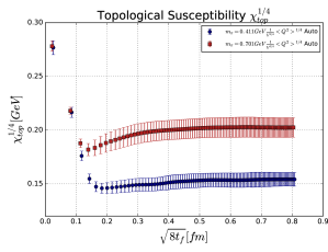
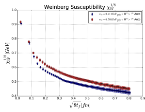
Figure 1: Topological (left) and Weinberg (right) susceptibilities in GeV, plotted against the flow-time radius $\sqrt{8t_{f}}$. Blue and red points are the $m_{\pi}=411,701$ MeV results respectively. Errors were estimated using the autocorrelation analysis technique described in Wolff:2003sm .

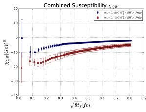
Figure 2: Cross correlation $\braket{Q\mathcal{O}_{W}}$ in GeV⁶ against the flow-time radius $\sqrt{8t_{f}}$. Blue and red points are the $m_{\pi}=411,701$ MeV results respectively. Errors were estimated using an autocorrelation analysis technique described in Wolff:2003sm .

For the topological susceptibility results in the left of fig.1, at small flow-time radius (ftr) $\sqrt{8t_{f}}$ we observe the expected short-distance singularities, while as we approach ftr of the order of the lattice spacing $\sqrt{8t_{f}}\approx 0.1$ fm, we see the divergences already being suppressed, but discretisation effects causing a “dip” in the flow time dependence. Once the ftr is of the order of $4-5$ times the lattice spacing, $\sqrt{8t_{f}}\approx 0.4$ fm, as expected no more flow time dependence is observed for this quantity. The result can simply be read off from any of $\sqrt{8t_{f}}>0.4$ fm, as the results are constant and nearly identical in this range. Any residual flow-time dependence is just a lattice artifact and will vanish in the continuum limit.

The Weinberg susceptibility in the right plot of fig.1 also shows an indication of possible divergences at small $\sqrt{8t_{f}}$, but unlike the topological susceptibility, we observe a non-trivial flow-time dependence over the whole range of $\sqrt{8t_{f}}$. The analysis of the flow-time dependence for the Weinberg susceptibility is ongoing.

A potentially interesting quantity to analyze, to understand the flow-time dependence of the Weinberg operator, is the “cross correlation” between the topological charge $Q$ and the integrated Weinberg operator $\mathcal{O}_{W}$ shown in fig.2. On general grounds the Weinberg operator mixes under renormalization with the topological charge density Bhattacharya:2015rsa and such correlator can provide a useful tool to disentangle contributions to the flow-time dependence of the Weinberg operator itself.

5 Nucleon Observables in CP-breaking theory

In this section, we show how to calculate nucleon observables in a CP-violating vacuum from lattice QCD. Along with this, we show the preliminary results demonstrating this procedure for both the $\theta$ and Weinberg CP-violating contributions to the nucleon observables. The method for the $\theta$-term has been discussed in detail in Shindler:2015aqa .

To study nucleon observables in a CP-violating vacuum we use a perturbative approach treating every CP-violating operator as insertion in the nucleon correlation functions evaluated in the usual QCD CP-conserving vacuum Shintani:2005xg ; Shindler:2015aqa .

5.1 Nucleon Mixing Angle

To understand how the nucleon reacts to a theory that includes CP-violation, we can calculate the nucleon CP-violating mixing angle, $\alpha_{N}$, which tells us how much the nucleon spinor is modified when placed in the CP-violating vacuum Shintani:2005xg ; Shindler:2015aqa :

$$u^{\cancel{CP}}_{N}(\vec{p},s)=e^{i\alpha_{N}\gamma_{5}}u_{N}(\vec{p},s).$$ (4)

The leading contribution of a generic CP-violating local operator $\mathcal{O}$ evaluated at flow time $t_{f}$, to the mixing angle $\alpha_{N}^{(1)}$, can be estimated computing the ratio between

$$G^{(\mathcal{O})}_{2}(\Gamma;\vec{0},t,t_{f})=\sum_{\vec{x}}\mathrm{Tr}\left\{\Gamma\gamma_{5}\braket{N(\vec{x},t)\overline{N}\,(0)\mathcal{O}(t_{f})}\right\}\,,$$ (5)

and the standard nucleon two-point correlation function

$$\frac{G^{(\mathcal{O})}_{2}(\Gamma_{4};\vec{0},t,t_{f})}{G_{2}(\Gamma_{4};\vec{0},t)}\xrightarrow{t\gg 0}\alpha^{(1)}_{N}(t_{f}).$$ (6)

where $N(\vec{x},t)$ is an interpolating operator with the quantum numbers of a nucleon (proton and neutron in $N_{f}=2+1$), $\Gamma$ is used in the trace to project out specific spin combinations, and a Fourier transform from position to momentum space is used to analyze a nucleon of momentum $\vec{p}$. In our case, the CP-violating operator $\mathcal{O}$ is the topological charge and the integrated Weinberg operator. The flow time dependence needs to be analyzed in addition to the ground state saturation through a large source-sink separation $t\gg 0$.

5.2 CP-odd Form Factor $F_{3}$ and the Electric Dipole Moment

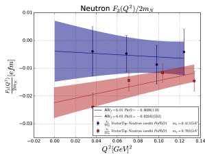
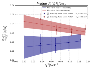
Figure 3: CP-odd vector form factor $F_{3}/2m_{N}$ in units of $\theta$ for the neutron (left) and proton (right), induced via the $\theta$-term CP-violating vacuum, plotted against transfer momentum $Q^{2}$. Blue and red points are the $m_{\pi}=411,701$ MeV results respectively. The linear fit to $Q^{2}\rightarrow 0$ is used to extract the value for the neutron and proton EDM $d_{n/p}$.

The CP-odd form factor for the nucleon $F_{3}(Q^{2})$, which is related to to the nucleon EDM via $d_{n/p}=F_{3}(0)/2m_{N}$, is only present in a theory that breaks CP-symmetry. Thus, to access this form factor from lattice QCD, we need to look at observables corresponding to form factors, in a CP-violating vacuum. In addition to standard two- and three- point correlation functions a modified three-point correlation of the form

$$G^{(\mathcal{O})}_{3}(\Gamma;\vec{p}^{\,\prime},t;\vec{q},\tau,t_{f})=\sum_{\vec{x},\vec{y}}e^{-i\vec{p}^{\,\prime}\cdot\vec{x}}e^{i\vec{q}\cdot\vec{y}}\mathrm{Tr}\left\{\Gamma\braket{N(\vec{x},t)\mathcal{J}_{\mu}(\vec{y},\tau)\overline{N}(0)\mathcal{O}(t_{f})}\right\},$$ (7)

is required to gain access to the CP-violating form factor $F_{3}(Q^{2})$ arising from a (flowed) CP-violating term $\mathcal{O}=Q\text{ or }\mathcal{O}_{W}$. After the matrix elements have been extracted from the three-point correlation functions (using fits in the region $t\gg\tau\gg 0$), the CP-odd form factor $F_{3}(Q^{2})$ can be disentangled from the CP-even form factors $F_{1,2}(Q^{2})$ by solving a system of equations. Since $F_{3}(0)$ cannot be extracted directly from $Q^{2}=0$, an extrapolation to $Q^{2}\rightarrow 0$ is required. We adopt a linear extrapolation in $Q^{2}$ following $\chi$PT results Ottnad:2009jw ; deVries:2010ah ; Mereghetti:2010kp .

In fig. 3 we show the $Q^{2}$ dependence of the CP-odd form factors induced by the $\theta$-term. The data show a signal for the heavy pion mass $m_{\pi}=701$ MeV while for the light pion mass $m_{\pi}=411$ MeV the results are consistent with a vanishing EDM within our statistical uncertainties. This results is not surprising because the $\theta$-EDM vanishes in the chiral limit in the continuum theory. The results from the proton and the neutron EDM differ in sign as well as the slope in $Q^{2}$. This is consistent with what is expected from $\chi$PT Ottnad:2009jw ; deVries:2010ah ; Mereghetti:2010kp .

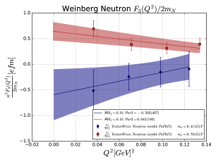
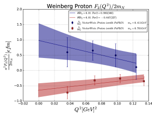
Figure 4: CP-odd vector form factor $F_{3}/2m_{N}$ in units of $\alpha_{W}/\Lambda^{2}$ for the neutron (left) and proton (right), induced via the Weinberg operator CP-violating vacuum, plotted against transfer momentum $Q^{2}$. Blue and red points are the $m_{\pi}=411,701$ MeV results respectively. The linear fit to $Q^{2}\rightarrow 0$ is used to extract the value for the neutron and proton EDM $d_{n/p}$.

In fig. 4 we show the same results for the CP-odd form factor induced by the Weinberg operator. Here $\chi$PT is less of a guide for the $Q^{2}$ and mass extrapolation because pion loops only enter at higher order deVries:2010ah . As a first attempt we still perform a simple linear extrapolation in $Q^{2}$. The data indicate that the EDM induced by the Weinberg operator changes sign when lowering the pion mass. As for the $\theta$-EDM the proton and neutron EDM have opposite sign as well as the slope in $Q^{2}$.

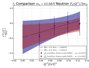
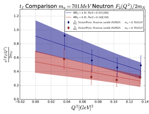
Figure 5: Flow time dependence from $t_{f}/a^{2}=4.01$ (blue) to $t_{f}/a^{2}=8.01$ (red) of the CP-odd vector form factor $F_{3}/2m_{N}$ in units of $\alpha_{W}/\Lambda^{2}$, induced via the Weinberg CP-violating vacuum, plotted against transfer momentum $Q^{2}$. Left and right plots show the $m_{\pi}=411,701$ MeV results respectively. The linear fit to $Q^{2}\rightarrow 0$ is used to extract the value for the neutron and proton EDM $d_{n/p}$.

An important aspect of the calculation of the EDM is the evaluation of the CP-odd operators at non-vanishing flow time. Excluding a region at small ftr, we expect that the $\theta$-EDM is independent on the flow time as it happens for the topological susceptibility and mixing angle (cfr. secs. 4.1, 5.1). We have verified that for the EDM in the range $4\leq t_{f}/a^{2}\leq 8$ the result is independent on the flow time. For the Weinberg EDM we would expect a non-trivial flow-time dependence stemming from the renormalization properties of the Weinberg operator (cfr. secs. 4.1, 5.1). The numerical data suggest that for the EDM induced by the Weinberg operator the flow-time dependence is of the same order of statistical accuracy of our calculation and is a little stronger for the heavier pion mass. This behavior can be observed in fig 5 where we show the flow-time dependence of the CP-odd form factors at 2 different flow times, $t_{f}/a^{2}=4.01$ and $8.01$.

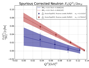
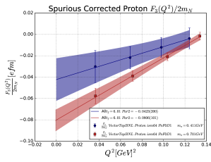
Figure 6: Corrections suggested by Abramczyk:2017oxr for the CP-odd vector form factor $F_{3}/2m_{N}$ in units of $\theta$ for the neutron (left) and proton (right), induced via the $\theta$-term CP-violating vacuum, plotted against transfer momentum $Q^{2}$. Blue and red points are the $m_{\pi}=411,701$ MeV results respectively. The linear fit to $Q^{2}\rightarrow 0$ is used to extract the value for the neutron and proton EDM $d_{n/p}$.

For the lighter pion mass in the left plot, there is no evidence of flow time dependence, besides the slight increase in the uncertainty. Whereas for the heavier pion mass result on the right, we see a $1\sigma$ discrepancy between the two extremes of flow time.

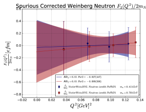
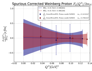
Figure 7: Corrections suggested by Abramczyk:2017oxr CP-odd vector form factor $F_{3}/2m_{N}$ in units of $\alpha_{W}/\Lambda^{2}$ for the neutron (left) and proton (right), induced via the Weinberg operator CP-violating vacuum, plotted against transfer momentum $Q^{2}$. Blue and red points are the $m_{\pi}=411,701$ MeV results respectively. The linear fit to $Q^{2}\rightarrow 0$ is used to extract the value for the neutron and proton EDM $d_{n/p}$.

We have also analyzed the numerical data following ref. Abramczyk:2017oxr . The results are shown in fig. 7. We observe that the corrections suggested in Abramczyk:2017oxr flip the sign of the $\theta$-EDM (and the slope in $Q^{2}$) and make the Weinberg EDM vanish for all pion masses and $Q^{2}$. We are currently incresing our statitics and running an additional pion mass to improve our analysis.

5.3 Conclusion

In this proceeding, we have obtained preliminary results for the $\theta$ and Weinberg EDM with $N_{f}=2+1$ dynamical gauge configurations at $2$ pion masses. We have defined the CP-odd local operators using the gradient flow for the gauge fields. We have treated the CP-sources in a perturbative manner allowing us to use existing QCD gauge configurations. For the $\theta$-EDM we clearly see a signal at the heavier pion mass while the lightest pion mass is still consistent with zero. Both the sign of the EDMs and the slopes in $Q^{2}$ of the CP-odd form factors are consistent with $\chi$PT. For the Weinberg EDM we see a clear signal at both pion masses, but the observed pion-mass dependence is not was is expected from $\chi$PT. The signal is washed out after applying the corrections of ref. Abramczyk:2017oxr and we see no signal at both pion masses.

It is interesting to notice that the flow-time dependence of the $\theta$-EDM is absent in the large range $4\leq t_{f}/a^{2}\leq 8$. We also observe no flow-time dependence for the Weinberg EDM indicating, most likely, that the variation of the Weinberg operator with the flow time due to its renormalization properties is below our statistical accuracy. To improve our determination we are currently increasing our statistics and using a third pion mass in our calculation.

References

- (1) C. Patrignani et al. (Particle Data Group), Chin. Phys. C40, 100001 (2016)
- (2) B. Graner, Y. Chen, E.G. Lindahl, B.R. Heckel, Phys. Rev. Lett. 116, 161601 (2016), [Erratum: Phys. Rev. Lett.119,no.11,119901(2017)], 1601.04339
- (3) C. Alexandrou, A. Athenodorou, M. Constantinou, K. Hadjiyiannakou, K. Jansen, G. Koutsou, K. Ottnad, M. Petschlies, Phys. Rev. D93, 074503 (2016), 1510.05823
- (4) Guo, F. -K. and Horsley, R. and Meißner, U. -G. and Nakamura, Y. and Perlt, H. and Rakow, P. E. L. and Schierholz, G. and Schiller, A. and Zanotti, J. M., Phys. Rev. Lett. 115, 062001 (2015), 1502.02295
- (5) S. Weinberg, Phys. Rev. Lett. 63, 2333 (1989)
- (6) S. Aoki et al. (PACS-CS), JHEP 08, 101 (2010), 1006.1164
- (7) M.G. Beckett, P. Coddington, B. JoÃ, C.M. Maynard, D. Pleiter, O. Tatebe, T. Yoshie, Computer Physics Communications 182, 1208 (2011)
- (8) S. Gusken, Nucl. Phys. Proc. Suppl. 17, 361 (1990)
- (9) Lüscher, Martin and Weisz, Peter, JHEP 02, 051 (2011), 1101.0963
- (10) M. Bruno, S. Schaefer, R. Sommer (ALPHA), JHEP 08, 150 (2014), 1406.5363
- (11) A. Chowdhury, A. Harindranath, J. Maiti, P. Majumdar, JHEP 02, 045 (2014), 1311.6599
- (12) Lüscher, Martin, JHEP 08, 071 (2010), [Erratum: JHEP03,092(2014)], 1006.4518
- (13) S. Borsanyi et al., JHEP 09, 010 (2012), 1203.4469
- (14) U. Wolff (ALPHA), Comput. Phys. Commun. 156, 143 (2004), [Erratum: Comput. Phys. Commun.176,383(2007)], hep-lat/0306017
- (15) T. Bhattacharya, V. Cirigliano, R. Gupta, E. Mereghetti, B. Yoon, Phys. Rev. D92, 114026 (2015), 1502.07325
- (16) A. Shindler, T. Luu, J. de Vries, Phys. Rev. D92, 094518 (2015), 1507.02343
- (17) E. Shintani, S. Aoki, N. Ishizuka, K. Kanaya, Y. Kikukawa, Y. Kuramashi, M. Okawa, Y. Tanigchi, A. Ukawa, T. Yoshie, Phys. Rev. D72, 014504 (2005), hep-lat/0505022
- (18) Ottnad, K. and Kubis, B. and Meißner, U. -G. and Guo, F. -K., Phys. Lett. B687, 42 (2010), 0911.3981
- (19) J. de Vries, R.G.E. Timmermans, E. Mereghetti, U. van Kolck, Phys. Lett. B695, 268 (2011), 1006.2304
- (20) E. Mereghetti, J. de Vries, W.H. Hockings, C.M. Maekawa, U. van Kolck, Phys. Lett. B696, 97 (2011), 1010.4078
- (21) M. Abramczyk, S. Aoki, T. Blum, T. Izubuchi, H. Ohki, S. Syritsyn, Phys. Rev. D96, 014501 (2017), 1701.07792