High Level Magnetic Activity Nature of an Eclipsing Binary KIC 12418816

Abstract

We present comprehensive spectroscopic and photometric analysis of the detached eclipsing binary KIC 12418816, which is composed of two very similar and young main sequence stars of spectral type K0 on a circular orbit. Combining spectroscopic and photometric modelling, we find masses and radii of the components as 0.88$\pm$0.06 $M_{\odot}$ and 0.84$\pm$0.05 $M_{\odot}$, and 0.85$\pm$0.02 $R_{\odot}$, and 0.84$\pm$0.02 $R_{\odot}$ for the primary and the secondary, respectively. Both components exhibit narrow emission features superposed on the cores of the Ca ii H&K lines, while $H_{\alpha}$ and $H_{\beta}$ photospheric absoprtion is more completely infilled by broader emission. Very high precision $Kepler$ photometry reveals remarkable sinusoidal light variation at out-of-eclipse phases, indicating strong spot activity, presumably on the surface of the secondary component. Spots on the secondary component appear to migrate towards decreasing orbital phases with a migration period of 0.72$\pm$0.05 year. Besides the sinusoidal variation, we detect 81 flares, and find that both components possess flare activity. Our analysis shows that 25 flares among 81 come exhibit very high energies with lower frequency, while the rest of them are very frequent with lower energies.

1 Introduction

Sinusoidal variations at out-of-eclipses in the light curves of YY Gem were observed by Kron (1952) for the first time in the literature. This unexpected phenomenon, called as BY Dra syndrome, was explained by Kunkel (1975) as a fact that was caused by heterogeneous temperature distribution, known today as the stellar spot activity on the surface of the star. This discovery demonstrated that UV Ceti type stars also exhibit spot activity. UV Ceti stars are cool dwarf stars on the main sequence possessing flare activity, which is observed as sudden and rapid increase of the stellar flux. The flare activity was discovered during the solar observations by R. C. Carrington and R. Hodgson on September 1, 1859 (Carrington, 1859; Hodgson, 1859). In the literature lots of studies, such as Kowalski et al. (2013), have been carried out since the first flare observation, the general view of the flare activity has been revealed. Nevertheless, it has not been yet understood some details of the flare and its process. In general, stellar flare activity observed on the dMe stars is modelled on the basis of the solar flare event, known as the standard solar flare model (Gershberg, 2005). Both stellar spot and flare activities are important in respect to the stellar evolution, because remarkable mass loss is occurred as a results of these activities (Benz & Güdel, 2010). The red dwarf population rate is about 65% in our Galaxy, while seventy-five percent of them possess flare activity (Rodono, 1986). This means that the population rate of UV Ceti type stars in our Galaxy is about 48.75%. However, it is well known for several decades that the general population rate of UV Ceti type stars is incredibly high in the young stellar clusters, such as the open clusters and the associations (Mirzoian, 1990; Pigatto, 1990). In addition, their population rate decreases as the cluster age increases. Considering the mass loss caused by stellar flare activity, this situation can be explained by the Skumanich law (Skumanich, 1972; Pettersen, 1991; Stauffer, 1991; Marcy & Chen, 1992). Although several studies and projects on the magnetic activity occurring on the stars have been accomplished so far, authors have been faced with some unexplained phenomena. One of them is the active longitude migration. For instance, Berdyugina & Usoskin (2003) found two stable active longitudes separated by 180° from each other on the surface of sun. According to them, these longitudes are exhibiting semi-rigid behaviour. On the other hand, these longitudes migrate regularly in time and they are not persistent active structures (Lopez Arroyo, 1961; Stanek, 1972; Bogart, 1982). The difference between the regular activity oscillations of these longitudes, which is so called the flip-flop, is very important in terms of the north-south asymmetry exhibited by the magnetic topology of the star. Furthermore, calculating angular velocities of these longitudes enlightens the latitudinal rotational velocities of spots and spot groups.

Besides the stellar spot activity, another unexplained phenomenon is also observed in case of the stellar flares. For instance, it is not absolutely known yet why there are differences between the flare energy limits for the stars from different spectral types. In the first place, the highest flare energy detected on the Sun increased up to $10^{30}$-$10^{31}$ erg, which is generally obtained from the most powerful solar flares, known as two-ribbon flares (Gershberg, 2005; Benz, 2008). The highest level of flare energy obtained in case of the Sun is the general value detected for the flares observed in RS CVn binaries (Haisch et al., 1991). However, flare energy range is a bit larger in case of red dwarfs. Detected minimum flare energy is about $10^{28}$ erg, while the observed maximum energy is about $10^{34}$ erg for dMe stars (Haisch et al., 1991; Gershberg, 2005). Apart from all these stars, the highest energy emitting in a flare event is found from the flares of the stars in young clusters such as the Pleiades cluster and Orion association. The flare energies obtained from these stars can reach $10^{36}$ erg (Gershberg & Shakhovskaia, 1983). Considering the standard solar flare model, if there is a difference between the flare energy level, similar difference is expected for the other effects of the flare event. In fact, observations demonstrated this expectancy, indicating differences between mass loss rates among the stars exhibiting the flare activity (Gershberg, 2005). According to the recent studies, the mass loss rate of UV Ceti type stars is about $10^{-10}$ $M_{\odot}$ per year due to flare like events, while the solar mass loss rate is about $2\times 10^{-14}$ $M_{\odot}$ per year (Gershberg, 2005). The difference between the mass loss ratios is also seen between the flare energy levels of the solar and stellar cases.

In spite of all these differences, flare events occurring on stars from different types are generally explained by the standard solar flare model, in which the main energy source is assumed as magnetic reconnection process (Gershberg, 2005; Hudson & Khan, 1996). However, to understand the whole view of the flare events, parameters, which cause these differences and similarities (among singularity, binarity, mass, age, etc.), should be identified. At that point, eclipsing binaries with a flaring component are very critical, because physical parameters of a star can be easily determined with light curve modelling. In these analyses, the main problem is the initial parameters, especially mass ratio of components and surface temperature of the primary component. In addition, to reach the real view about flare events, number of samples must be increased.

KIC 12418816 was listed in the USNO-A2.0 Catalogue by Monet (1998) to the first time in the literature. In this catalogue, B and R band magnitudes of the system were listed as 13$\aas@@fstack{m}$9 and 12$\aas@@fstack{m}$6, respectively. The brightnesses in the infrared filters $J$, $H$ and $K$ were given as 10$\aas@@fstack{m}$872, 10$\aas@@fstack{m}$400 and 10$\aas@@fstack{m}$271, respectively (Zacharias et al., 2004). The system was classified as an eclipsing Algol with a period of 1$\aas@@fstack{d}$521925 (Watson, 2006), and with no third light contribution. Coughlin et al. (2011) tried to determine the parameters of the system for the first time in the literature, and they found that the system possesses a light curve with amplitude of 0$\aas@@fstack{m}$581 and an orbital inclination of 87$\aas@@fstack{\circ}$12. They also found representative effective temperature of the system as 4583 K, while the individual temperatures were found as 4603 K and 4563 K for the primary and the secondary component, respectively. In the same study, the mass and radius are given as 0.78 $M_{\odot}$ and 0.81 $R_{\odot}$ for the primary component, and 0.77 $M_{\odot}$ and 0.80 $R_{\odot}$ for the secondary component. Moreover, Slawson et al. (2011) gave log $g$ and $E(B-V)$ value of the system as 4.491 and 0$\aas@@fstack{m}$029, respectively. Both Pinsonneault et al. (2012) and Huber et al. (2014) confirmed previously given log$g$ value and found $[Fe/H]=-1.51$, while they indicated a bit different temperature values compared to the previous studies. More recently, Armstrong et al. (2014) computed the temperature as 4909 K for the primary component and 4796 K for the secondary component, which are based on spectral energy distribution fitting. Morton et al. (2016) recently found an effective temperature of 4998 K with $[Fe/H]=-0.08$, and they estimated the age of the system as log(age)=9.53 Gyr in the distance of 175 pc.

In this study, we figure out the nature of KIC 12418816 via medium resolution spectroscopy and very high precision space photometry from $Kepler$ spacecraft. In the next section, we summarize source of observational data and reduction processes. Section 3 comprises spectroscopic and photometric modelling of the system, including analysis of spot activity and flares. In the final section, we summarize and discuss our findings in the scope of physical properties and magnetic activity nature of the components.

2 Observations and data reductions

2.1 $Kepler$ photometry

We use detrended and normalized short cadence (58.89 seconds) and long cadence (29.4 minutes) $Kepler$ photometry of KIC 12418816 available at $Kepler$ eclipsing binary catalogue (Slawson et al., 2011; Prša et al., 2011). The catalog includes 42325 data points obtained in short cadence photometry, and 57521 data points in long cadence photometry. However, twelfth and thirteenth quarters are missing in the long cadence data set, thus we extracted data of missing quarters from Mikulski Archive for Space Telescopes (MAST) database. We considered simple aperture photometry (SAP) fluxes for these quarters and followed the procedure described by Slawson et al. (2011) to detrend SAP fluxes. The final long cadence data set includes all 17 Quarters of Kepler mission, with 65192 data points in total, and provides almost continuous $\sim$4 years of photometry. Slawson et al. (2011) estimated one percent of contamination due to the other sources close to the KIC 12418816.

2.2 Optical spectroscopy

We carried out optical spectroscopic observation of the system with 1.5-m Russian–Turkish telescope equipped with Turkish Faint Object Spectrograph Camera (TFOSC) at Tubitak National Observatory. The instrumental set-up provided medium resolution échelle spectra with a resolution of R = $\lambda/\Delta\lambda$ $\sim$2500 around 6500 Å, covering wavelengths between 3900 Å and 9100 Å in 11 échelle orders. All spectra were recorded with a back illuminated 2048 $\times$ 2048 pixels CCD camera with a pixel size of 15 $\times$ 15 $\mu m^{2}$.

We recorded eleven spectra of our target star between 2014 and 2016 observing seasons. Signal-to-noise ratio (SNR) of observed spectra were between 50 and 100 depending on atmospheric conditions and exposure time. In addition to target star observations, we obtained high SNR optical spectra of 54 Psc (HD 3651, K0V), HD 190404 (K1V) and $\tau$  Cet (HD 10700, G8.5V) and used these spectra as spectroscopic comparison and radial velocity template.

We followed typical échelle spectra reduction steps for reducing observations. We first removed instrumental noise from all observed frames by using average of nightly obtained bias frames. Then we obtained average flat-field image from bias corrected halogen lamp frames and normalized the average flat-field image to the unity. We divided all science and Fe-Ar calibration lamp frames by the normalized flat-field frame and applied scattered light correction and cosmic ray removal to all flat-field corrected frames, thus we obtained reduced calibration lamp and science frames. We extracted spectra from reduced science frames and applied wavelength calibration to them. Finally, we normalized all science spectra to the unity by using cubic spline function. We applied all reduction steps in IRAF environment.

3 Analysis

3.1 Light elements and $O-C$ diagram

We start analysis with determination of mid-eclipse times in long cadence data set. We fit third or fourth order polynomial to each eclipse to determine mid-eclipse time. Order of polynomial depends on the shape and asymmetry of the corresponding eclipse. Then we use determined eclipse times to construct an $O-C$ diagram via initial light elements given in $Kepler$ eclipsing binary catalog (Equation 1), and obtain improved light elements by applying a linear fit to the $O-C$ data.

$$T_{0}{\rm(BJD)}=2,454,954.742983+1\aas@@fstack{d}5218703\ \times\ E.$$ (1)

Since each eclipse includes only a few data points, polynomial fits to the eclipses leads to lower precision, hence a scatter with an amplitude of 0.005 day in $O-C$ diagram. Nevertheless, we continue with the improved light elements for further spectroscopic orbit and light curve modelling. After we achieve the best light curve model for the eclipsing binary, we divide the long cadence data into subsets, where each subset covers only a single orbital cycle, and re-calculate each eclipse time in a single cycle of each subset by keeping all light curve model parameters fixed, but only adjusting ephemeris time. By this way, we are able to determine eclipse times and their statistical errors reasonably and more precisely. For primary eclipses, this process was pretty straightforward, while for the secondary eclipses we needed to change the role of components (thus role of eclipses) in the light curve model and shifted each light curve by 0.5 in phase. We repeat this process iteratively until we achieve self consistent light elements (Equation 2). These light elements are adopted for further analysis.

$$T_{0}{\rm(BJD)}=2,454,954.74366(3)+1\aas@@fstack{d}52187051(5)\ \times\ E.$$ (2)

The residuals were derived according to the linear fit obtained from the final eclipse times leads to $O-C~{}II$ diagram shown in Figure 1. There is a wave like variation in a form of an irregular sinusoidal wave with an amplitude of 0.001 day. According to the discussions in Balaji et al. (2015) and Tran et al. (2013), the variation is possibly due to the strong chromospheric activity of both components (see Section 3.5).

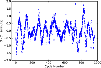
Figure 1: $O-C$ diagram of the eclipse times.

3.2 Radial velocities and spectroscopic orbit

We use 54 Psc as radial velocity template, and cross-correlate it with each of eleven spectra of KIC 12418816 in order to determine radial velocities of the components. We follow cross-correlation procedure described by Tonry & Davis (1979) via $fxcor$ task under IRAF environment. We use absorption lines between 5000 Å and 6500 Å, except broad lines (e.g. Na I D lines) and strongly blended lines, to calculate cross-correlation function. We are able to detect strong and clear cross-correlation signals from both components. In Figure 2, we plot cross-correlation functions for two spectra obtained at orbital quadratures.

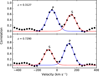
Figure 2: Cross-correlation functions of two spectra obtained at orbital quadratures. The letter $\phi$ denotes corresponding orbital phase. P and S indicate the primary component and the secondary component, respectively.

Table 1: Brief information on observed spectra, measured radial velocities and their corresponding standard errors ($\sigma$) in km s^-1.

HJD	Orbital	Exposure	Primary		Secondary
(24 00000+)	Phase	time (s)	Vr	$\sigma$	Vr	$\sigma$
56844.4944	0.7290	3600	96.7	5.2	-118.1	8.0
56845.3827	0.3127	3600	-111.7	5.1	91.0	8.8
56845.4254	0.3407	3600	-101.6	6.0	84.3	8.7
56889.2664	0.1481	2400	-103.5	7.4	80.3	11.0
56890.3491	0.8595	3600	70.2	5.6	-100.1	9.7
56890.5051	0.9620	2400	18.0	6.3	-41.9	7.3
57592.3044	0.1045	1200	-81.4	7.3	69.3	10.7
57601.3201	0.0287	3600	-22.0	4.0	—	—
57601.4964	0.1445	3600	-97.5	6.9	75.1	9.3
57616.4126	0.9457	3600	20.0	7.2	-52.8	11.4
57617.4558	0.6312	3600	69.7	5.7	-90.5	10.0

We tabulate measured radial velocities in Table 1, together with brief information on observed spectra. Preliminary inspection of long cadence light curve indicate no considerable eccentricity for the orbit, hence we determine spectroscopic orbit of the system under circular orbit assumption. Application of Levenberg-Marquardt algorithm (Levenberg, 1944; Marquardt, 1963), and Markov chain Monte Carlo simulations via $Python$ package $emcee$ (Foreman-Mackey et al., 2013) to the measured radial velocities and their errors, which is done via a simple script written in $Python$ language, leads to the spectroscopic orbit parameters tabulated in Table 2. We plot phase-folded radial velocities and theoretical spectroscopic orbit in Figure 3, together with the residuals from the best-fitting model.

Table 2: Spectroscopic orbital elements of KIC 12418816. $M{{}_{1}}$ and $M{{}_{2}}$ denote the masses of the primary and the secondary component, respectively, while $M$ shows the total mass of the system.

Parameter	Value
$P_{\rm orb}$ (day)	1.52187051 (fixed)
$T_{\rm 0}$ (HJD2454+)	954.74366 (fixed)
$\gamma$ (km s-1)	$-10.3\pm 1.3$
$K_{1}$ (km s-1)	108.5$\pm$2.3
$K_{2}$ (km s-1)	112.9$\pm$3.9
$e$	0 (fixed)
$a\sin i$ ($R_{\odot}$)	6.66$\pm$0.14
$M\sin^{3}i$ ($M_{\odot}$)	1.710$\pm$0.079
Mass ratio ($q=M{{}_{2}}/M{{}_{1}}$)	0.96$\pm$0.04
rms1 (km s-1)	4.1
rms2 (km s-1)	4.6

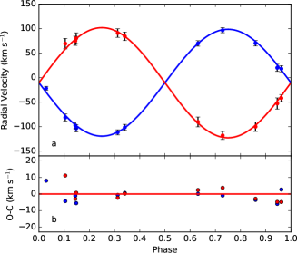
Figure 3: a) Observed radial velocities of the primary and the secondary (blue and red filled circles, respectively), and their corresponding theoretical representations (blue and red curves). b) Residuals from theoretical solution.

3.3 Spectral type and features

Before proceeding with the spectral classification, we notice exceptional behaviour of Balmer lines $H_{\alpha}$ and $H_{\beta}$, which are not in absorption, but filled with emission and embedded into the continuum in our medium resolution spectra. There are strong emission features in Ca ii H&K lines, where we can clearly detect emission from both components. In Figure 4, we show these spectral lines.

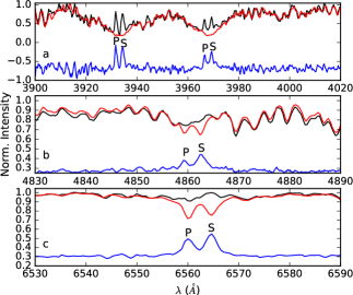
Figure 4: Ca ii H&K ($a$), $H_{\beta}$ ($b$) and $H_{\alpha}$ ($c$) regions. Emission in $H_{\alpha}$ and $H_{\beta}$ is clearer in residuals from model spectrum. Components are marked with P and S, denoting the primary and the secondary component, respectively. Black line shows the observed spectrum, red line is the model for the composite spectrum (see the text), and blue line is the difference between the observation and the model, which is shifted upwards by 0.3 for the sake of simplicity.

We use high SNR spectra of 54 Psc (K0V, Gray et al., 2003), HD 190404 (K1V, Frasca et al., 2009) and $\tau$  Cet (G8.5V, Gray et al., 2006) as comparison templates to estimate the spectral type of the components. Spectral types of these stars were reliably determined via high resolution spectroscopic observations in the given references. Among eleven spectra of KIC 12418816, we select the spectrum recorded on the night of HJD 24 56845, where we can clearly separate spectral lines of both components. Then, we calculate composite spectrum for each binary combination of template stars, (54 Psc+HD 190404, HD 190404+$\tau$  Cet, HD 190404+HD 190404, etc.) and compare each calculated composite spectrum with the selected spectrum of KIC 12418816. For a given binary combination, we first apply proper radial velocity shift to the spectrum of each template star to match their spectral lines to the lines of corresponding component along the wavelength. Then, we calculate resulting composite spectrum by considering the luminosity ratio of the components that we find from light curve modelling. We iterate this process until we achieve agreement between spectral types, and luminosity ratio found from light curve modelling. Among all possible binary configurations of the template stars mentioned above, 54 Psc+54 Psc configuration with a luminosity ratio ($L_{1}/L_{2}$) of 1.095 (see Section 3.4) provides fairly good representation of the observed spectrum, and indicates K0V spectral type for both components of KIC 12418816 with solar metallicity. K0V spectral type corresponds to 5250 K of effective temperature (Gray, 2005). Considering S/N of observed spectra and resolution of TFOSC, we estimate the uncertainty in effective temperature as 200 K. In Figure 5, we show different portions of selected KIC 12418816 spectrum, and calculated composite spectrum from the combination of 54 Psc + 54 Psc.

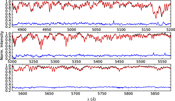
Figure 5: Different portions of selected KIC 12418816 spectrum. Meaning of the colours are the same as in Figure 4. Composite spectrum is for 54 Psc + 54 Psc configuration. Residuals between the selected and composite spectra are shifted upwards by 0.3 for the sake of simplicity.

Estimated temperature of the primary component, $T_{1}$, differs more than 250 K from the temperature estimated by Armstrong et al. (2014) (4909 K) and Morton et al. (2016) (4998 K). Armstrong et al. (2014) estimated the temperature via spectral energy distribution of the star, which is based on photometric measurements in different bands. Morton et al. (2016) used 3D linear interpolation in mass-[Fe/H]-age parameter space for a given stellar model grid. Since these approaches are not as precise as spectroscopic methods in terms of temperature determination, it is not surprising to find considerably different temperature in case of KIC 12418816. Our temperature estimation is based on fitting of observed spectra in a wide optical wavelength range, which provides more precise and reliable atmospheric parameters, compared to the above-mentioned methods.

3.4 Light curve modelling

We focus on long cadence photometry to obtain radiative and physical properties of KIC 12418816. Before modelling, we create phase-binned average light curve of the binary by using light the elements given in Equation 2 and 65192 long cadence data point. Phase binning step is 0.002 and the average light curve includes 500 data points. Figure 6 panel $a$ and $b$ show different time ranges from long cadence photometry, where considerable differences in the shape of light maxima, and flares are observed.

We model the phased and binned light curve with 2015 version of the Wilson-Devinney code (Wilson & Devinney, 1971; Wilson & Van Hamme, 2014). The phase-binned average light curve clearly points to detached configuration, while phases of eclipses (1.0 and 1.5 for the primary and the secondary eclipses, respectively) indicate circular orbit for the binary (Figure 6 panel $c$, black filled circles). The most critical two parameters of light curve modelling, i.e. mass ratio ($q=M_{2}/M_{1}$) and effective temperature of the primary component ($T_{1}$) have already been determined in previous sections, thus modelling process is pretty straightforward and only requires adjustment in phase shift, orbital inclination ($i$), effective temperature of the secondary component ($T_{2}$), dimensionless potentials of the components ($\Omega_{1}$ and $\Omega_{2}$) and luminosity of the primary component ($L_{1}$). Albedo ($A_{1}$ and $A_{2}$) and gravity darkening coefficients ($g_{1}$ and $g_{2}$) are set to their typical values for convective stars, and square root limb darkening law (Klinglesmith & Sobieski, 1970) for $Kepler$ passband was adopted, where the limb darkening coefficients ($x_{1}$, $x_{2}$, $y_{1}$, $y_{2}$) and bolometric limb darkening coefficients ($x_{1bol}$, $x_{2bol}$, $y_{1bol}$, $y_{2bol}$) are taken from tables of van Hamme (1993). Considering circular orbit, we assume synchronized rotation for the components, thus fixed rotation parameter of components ($F_{1}$ and $F_{2}$) to the unity. We tabulate parameters of best-fitting light curve model in Table 3, and plot the model in Figure 6 panel $c$ with red curve.

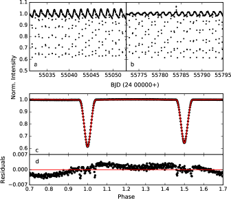
Figure 6: Panel $a$ and $b$ show different parts of long cadence data. Phase binned average light curve is in panel $c$ (black filled circles) together with the best-fitting light curve model (red curve). Residuals from the model is shown in panel $d$.

Table 3: Parameters of best-fitting light curve model for KIC 12418816. $\langle r_{1}\rangle$ and $\langle r_{2}\rangle$ denote mean fractional radii of the primary and the secondary component, respectively. Internal errors of the adjusted parameters are given in parentheses for the last digits. Asterisk symbols in the table denote fixed value for the corresponding parameter. Note that we adopt the uncertainty of $T_{1}$ for $T_{2}$ as well, since the internal error of $T_{2}$ is unrealistically small ($\sim$2 K).

Parameter	Value
$q$	0.96*
$T_{1}(K)$	5250*
$g_{1}$, $g_{2}$	0.32*, 0.32*
$A_{1}$, $A_{2}$	0.5*, 0.5*
$F_{1}$ = $F_{2}$	1.0*
phase shift	$-$0.00003 (2)
$i~{}(^{\circ})$	86.53 (1)
$T_{2}(K)$	5162 (200)
$\Omega_{1}$	8.805 (31)
$\Omega_{2}$	8.606 (32)
$L_{1}$/($L_{1}$+$L_{2})$	0.525 (4)
$x{{}_{1}bol},x{{}_{2}bol}$	0.646*, 0.645*
$y{{}_{1}bol},y{{}_{2}bol}$	0.177*, 0.172*
$x{{}_{1}},x{{}_{2}}$	0.744*, 0.747*
$y{{}_{1}},y{{}_{2}}$	0.176*, 0.162*
$\langle r_{1}\rangle,\langle r_{2}\rangle$	0.1277 (5), 0.1266 (5)
Model rms	6.7 $\times$ 10-3

Combined spectroscopic orbit and light curve modelling results yield physical parameters of the system listed in Table 4, indicating that the system is composed of two stars very similar to each other in terms of physical parameters and evolutionary status. We plot the components on $Log~{}T_{eff}-Log~{}L/L_{\odot}$ plane in Figure 7.

Table 4: Absolute physical properties of KIC 12418816. Error of each parameter is given in paranthesis for the last digits.

Parameter	Primary	Secondary
Spectral Type	K0V	K0V
[Fe/H]	0.0
Mass ($M_{\odot}$)	0.88(6)	0.84(5)
Radius ($R_{\odot}$)	0.85(2)	0.84(2)
Log $L/L_{\odot}$	$-$0.303(68)	$-$0.340(69)
log $g$ (cgs)	4.521(15)	4.511(9)
$M_{bol}$ (mag)	5.51(17)	5.60(17)

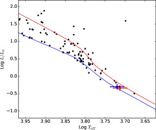
Figure 7: Components of KIC 12418816 (blue and red filled circles for the primary and the secondary component, respectively) in $Log~{}T_{eff}-Log~{}L/L_{\odot}$ plane. Blue and red lines denote ZAMS and TAMS, respectively (Pols et al., 1998). Black filled circles show positions of the components of detached eclipsing binaries, taken from Ibanoǧlu et al. (2006).

3.5 Stellar cool spot activity

The available data indicate that the system exhibits also sinusoidal variations at out-of-eclipses in light curves. The sinusoidal variation is so distinctive that it is easily noticed in whole light curve, in spite of occasional flares and much deeper eclipses. Considering the surface temperatures of the components of the system, it is possible that the sinusoidal variation must be caused by the rotational modulation due to the cool stellar spots. Short cadence data plotted in Figure 8 clearly shows that the shape and amplitude of the sinusoidal variation are absolutely changed from one cycle to the next one. This situation indicates that the active regions on the components are rapidly evolving and also migrating on the surfaces of the components.

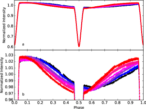
Figure 8: a) The light curves obtained from the available short cadence data are plotted versus phase. b) The same light curve is plotted by expanding the intensity axis to show the sinusoidal variations clearly.

Before examining out-of-eclipse variations, we first removed the best-fitting eclipsing binary model from the long cadence data. In practice, we follow the method described in Section 3.1, which was used to determine precise eclipse times. In the method, we obtain residuals from the theoretical model, after fitting the ephemeris time. This procedure eliminates any shift in the ephemeris time, which could arise from any physical reason, such as third body or spot activity, thus provides residuals precisely. After obtaining the residuals from whole long cadence data, we then removed all visually-determined large flares from the residuals. We use the final residuals for further analysis in this section. Finally, we fit third or fourth degree polynomial to the data points around the deepest light minimum in an orbital cycle to determine the corresponding time of that minimum. As in mentioned in Section 3.1 order of polynomial is chosen according to the shape and asymmetry of the light curve for a given cycle. After determining the minima times, we calculate orbital phase of each minimum using the light elements given in Equation 2.

In Figure 9 panel $a$, we plot the calculated phases of minima (hereafter $\theta_{min}$) versus Barycentric Julian Date. $\theta_{min}$ values are clearly migrating toward the decreasing values time by time, and this migration repeats itself more than six times between orbital phases 0.0 and 1.0, through the 4 years of long cadence data. In panel $a$, as the time progresses, $\theta_{min}$ values approach to $\theta_{min}=0.0$ and then jump to $\theta_{min}=1.0$. In order to see migration without interruption, one needs to add a proper integer to the $\theta_{min}$ values occurred before each jump, so that all $\theta_{min}$ values appear on a trend without any discontinuity. By this way, we obtain adjusted $\theta_{min}$ values (thus adjusted migration movement). We plot the adjusted $\theta_{min}$ values versus Barycentric Julian Day in Figure 9 panel $b$. Here, we note that a jump of 0.5 in phase is observed for the $\theta_{min}$ approximately around BJD 24 55760. This behaviour is generally observed in the switching of the deeper minimum in the light curve by 0.5 in phase, which is commonly called as Flip-Flop in the literature (Berdyugina & Järvinen, 2005).

Using the least-squares method, we derived the best linear fit (Equation 3) for adjusted phases of the times of minima, where $\theta_{min}$ is an adjusted phase for the minimum time, while $\tau$ is the Barycentric Julian Date, taking $\tau_{0}$ as 24 54954.633527 that corresponds to the time of the first minimum found from the residuals. The numbers in brackets in Equation 3 denote the statistical error for the coefficients and the constant, for their last digits.

$$\theta_{min}=-0.003772(6)\times[\tau-\tau_{0}]+6.782(5)$$ (3)

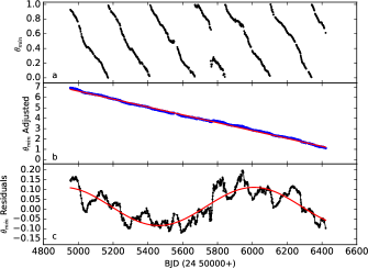
Figure 9: a) The phases of minima times of the sinusoidal variations ($\theta_{min}$) are plotted versus the Barycentric Julian Date. b) Similar to $a$ but for adjusted phases. Red line shows linear fit to the adjusted phases. c) $\theta_{min}$ residuals derived according to the linear fit given in Equation 3. The red curve represents a sine wave obtained as the best fit for the residuals.

With careful inspection of the Figure 9 panel $b$, slight deviation of the adjusted $\theta_{min}$ values around the linear fit can be noticed. We plot the residuals from the linear fit in Figure 9 panel $c$, which reveals a clear variation following two sine waves, one with a large amplitude and small frequency shown by a line in the figure, and another one with has small amplitude and high frequency.

3.6 Flare activity and the OPEA model

Apart from the rotational modulation of light curves caused by spot activity, both the long cadence and the short cadence data of KIC 12418816 demonstrate that the system exhibits flare activity with high frequency. In this respect, first of all, using the residual data parts without any instant brightness increase were modelled by the Fourier Transform for each cycle. Then, the fit models derived from these Fourier Transforms were taken as the quiescent levels. Following the process described by Dal & Evren (2010a, 2011b), the start and end points were determined for each flare. Finally, all flare parameters were computed with respect to the quiescent levels.

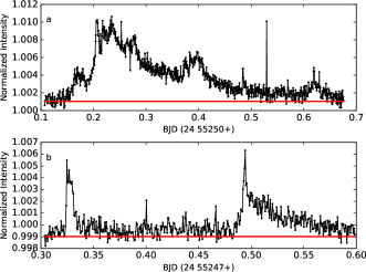
Figure 10: The flare light curve samples chosen from different parts of the short cadence data. In the figures, the filled circles represent the observations, while the red lines represent the light level assumed as the quiescent state of the star.

We detect 81 flares in total, where 73 of them are from the short cadence data, and 8 of them are from the long cadence data. We show two sample flares in Figure 10, which are detected from the short cadence data. For each flare, we first define beginning and end of the flare, and then compute the flare rise time ($\tau_{r}$), the decay time ($\tau_{d}$), amplitude of the flare maxima, and the flare equivalent duration ($P$). $P$ is defined as,

$$P=\int(\dfrac{I_{flare}-I_{0}}{I_{0}})dt$$ (4)

where $P$, $I_{0}$ and $I_{flare}$ are the flare-equivalent duration, the intensity of the star in the quiescent state and the intensity observed at the moment of the flare, respectively (Gershberg, 1972). We note that we do not compute the flare energies to be used in the following analyses, due to the reasons described in detail by Dal & Evren (2010a, 2011b). We tabulate computed parameters of 81 flares in Table 5.

Table 5: All the calculated parameters of flares detected from the short cadence observational data of KIC 12418816. The flares are separated into two groups, as Group 1 and Group 2.

Group1
Flare Time	$P$	$\tau_{r}$	$\tau_{r}$	Amplitude
BJD (24 00000+)	(s)	(s)	(s)	(Intensity)
55209.95848	182.4619	1765.4980	10592.5540	0.063
55246.31868	3.6229	411.9550	1176.9410	0.006
55247.32470	4.9478	353.1170	1588.8960	0.007
55248.05894	0.3060	58.9250	58.8380	0.000
55249.52404	0.3441	117.7630	176.5150	0.003
55249.88912	31.4420	176.5150	3060.1150	0.055
55250.23445	123.1273	6944.2270	30366.0580	0.010
55257.07293	1.7541	58.8380	117.6770	0.029
55257.35491	4.5288	294.1920	1353.5420	0.006
55257.67981	0.9500	58.8380	529.6320	0.002
55258.50397	4.5736	176.6020	1588.8960	0.009
55263.59266	3.2521	176.5150	1294.7040	0.006
55269.47012	0.2125	58.8380	58.9250	0.003
55269.49396	0.4468	117.6770	235.3540	0.005
55271.04285	1.1811	176.5150	411.9550	0.005
55273.88248	0.2896	176.5150	117.7630	0.003
55274.62083	105.0486	529.8050	23010.1340	0.008
55275.00771	1.5188	117.6770	706.2340	0.003
55279.04444	249.9872	5296.4930	14123.9810	0.071
55348.58201	103.8675	3531.0820	14124.1540	0.028
55377.57815	125.6882	1765.4980	15889.5650	0.023
55664.72893	171.9245	1765.4980	8827.4880	0.059
55705.41346	223.9744	3531.0820	28248.3070	0.022
55783.86009	258.5934	5296.4930	14123.8940	0.060
55837.19165	444.8300	7061.7310	14123.4620	0.124
Group2
Flare Time	$P$	$\tau_{r}$	$\tau_{r}$	Amplitude
BJD (24 00000+)	(s)	(s)	(s)	(Intensity)
55247.49429	10.6828	706.1470	5355.2450	0.007
55247.92544	2.2056	470.7940	1118.1020	0.005
55248.01808	1.1038	353.0300	706.2340	0.002
55248.17814	5.3484	1824.3360	5002.1280	0.001
55248.27418	1.7568	353.1170	882.7490	0.004
55248.36749	6.5505	1824.2500	3060.2020	0.002
55248.52824	2.9749	294.2780	1647.7340	0.004
55248.87425	2.0699	294.2780	1824.2500	0.000
55249.75562	5.5426	353.1170	3707.5100	0.001
55250.61928	7.6038	2883.6000	4884.4510	0.003
55251.01569	3.9503	1353.5420	2353.9680	0.001
55251.05179	4.4005	764.9860	1706.6590	0.005
55251.22344	20.1882	5590.5980	10592.8130	0.003
55251.35012	5.1587	353.1170	5473.0080	0.003
55252.20017	15.8413	1824.3360	11181.2830	0.006
55253.16395	6.1278	470.7940	3472.0700	0.003
55254.07802	0.2145	58.8380	294.1920	0.000
55254.10050	0.1640	58.8380	235.3540	0.000
55254.28032	4.7232	470.7940	3472.0700	0.002
55254.36069	1.0356	411.9550	588.4700	0.002
55257.11652	1.3689	411.9550	647.3090	0.003
55257.15194	1.0095	529.6320	353.1170	0.003
55257.86848	4.4334	529.6320	3295.5550	0.004
55257.91820	0.9397	294.2780	764.9860	0.002
55258.48217	1.1849	353.1170	588.4700	0.004
55258.66267	4.6701	1177.0270	2059.6900	0.003
55258.80094	14.3333	1471.2190	7473.8590	0.003
55258.92490	1.8988	588.4700	1412.3810	0.002
55260.24220	1.9206	235.3540	1647.8210	0.002
55260.45744	3.3707	294.2780	2412.8060	0.003
55261.83195	2.0364	235.3540	1530.0580	0.002
55261.92799	3.4647	1530.0580	2707.0850	0.002
55263.44009	1.6343	411.9550	1118.1020	0.002
55263.60901	0.7591	117.6770	470.8800	0.003
55264.36642	2.1965	353.1170	1059.2640	0.004
55264.59460	2.2930	353.0300	1059.3500	0.002
55265.29071	2.5882	294.1920	1294.7040	0.004
55265.31387	0.6201	176.5150	470.7940	0.002
55266.82598	6.7981	1118.1890	2471.6450	0.005
55267.17744	0.3133	176.5150	176.5150	0.003
55267.18425	0.9339	411.9550	529.6320	0.003
55267.35113	3.2132	235.4400	1471.2190	0.005
55267.69169	11.2563	353.1170	6473.4340	0.005
55268.44706	1.6236	411.9550	706.2340	0.003
55268.54106	10.1567	4531.4210	3177.8780	0.003
55270.06679	2.6880	176.5150	1235.8660	0.006
55270.26091	3.2616	117.6770	2059.6900	0.003
55270.29906	0.3316	58.8380	294.2780	0.002
55270.76018	1.1611	58.8380	941.5870	0.004
55270.80309	2.8562	470.7940	1942.0990	0.003
55272.16331	5.2687	823.9100	2883.6860	0.003
55272.20894	3.8012	1059.2640	2471.6450	0.002
55273.01268	2.6030	294.1920	1294.7040	0.004
55273.49832	7.3640	823.8240	11946.5280	0.006
55273.77350	26.7146	6885.3890	8709.8110	0.003
55274.54590	7.4994	2883.6000	4060.6270	0.002

Examining the relationships between the flare parameters, it was seen that the distribution of flare equivalent durations on the logarithmic scale versus flare total durations are varying in a rule. The distribution of flare equivalent durations on the logarithmic scale cannot be higher than a specific value for the star, and it is no matter how long the flare total duration is. Using the SPSS V17.0 (Green et al., 1996) and GrahpPad Prism V5.02 (Motulsky, 2007) programs, Dal & Evren (2010a, 2011b) demonstrated that the best function is the One Phase Exponential Association (hereafter $OPEA$) for the distributions of flare equivalent durations on the logarithmic scale versus flare total durations. The $OPEA$ function (Motulsky, 2007; Spanier & Oldham, 1987) has a Plateau term, and this makes it a special function in the analyses. The $OPEA$ function is defined by Equation 5,

$$y=y_{0}+(Plateau-y_{0})\times(1-e^{-k\times x})$$ (5)

where the parameter $y$ is the flare equivalent duration on a logarithmic scale, the parameter $x$ is the flare total duration as a variable parameter, according to the definition of Dal & Evren (2010a). In addition, the parameter $y_{0}$ is the flare-equivalent duration on a logarithmic scale for the least total duration, which means that the parameter $y_{0}$ is the least equivalent duration occurring in a flare for a star. Logically, the parameter $y_{0}$ does not depend on only flare mechanism occurring on the star, but also depends on the sensitivity of the optical system used for the observations. In this case, the optical system is the optical systems of the $Kepler$ Satellite. The parameter Plateau value is the upper limit for the flare equivalent duration on a logarithmic scale. Dal & Evren (2011b) defined Plateau value as a saturation level for a star in the observing band.

After we derive the $OPEA$ model for all 81 flares, we notice that the correlation coefficient squared ($R^{2}$) is very low, while the probability value ($p-value$) is very high. It means that the model does not perfectly fit the distributions. In fact, it seems that there are two arms in the distribution of flare equivalent durations on the logarithmic scale ($log~{}P$) versus flare total time ($\tau_{t}$) toward the higher equivalent durations. Particularly, this dissociation gets much clearer for the flares, whose total flare time is longer than 1700 s. The flares with total flare times smaller than 1700 s seems that they mazily locate together in the distribution of flare equivalent durations on the logarithmic scale. In this point, we derived two independent models for the flares with total flare times larger than 1700 s. Then, following these independent model trends we split also the flares with total flare times smaller than 1700 s into two groups. Hence, 25 flares were grouped as Group 1, while the rest of them were grouped as Group 2.

The independent samples t-test (hereafter t-test) (Dawson & Trapp, 2004; Wall & Jenkins, 2003) was used in the SPSS V17.0 and GraphPad Prism V5.02 software in order to test whether these two groups are really independent from each other. The main average of the equivalent durations in the logarithmic scale for the flares in the plateau level of Group 1 was calculated and found to be 2.253$\pm$0.064 s with standard deviation of 0.203 s, and it was found to be 1.020$\pm$0.065 s with standard deviation of 0.222 s for the flares in the plateau level of Group 2. This analyses also confirmed that the separation between two groups is statistically acceptable.

Finally, using the least-squares method, we derive the $OPEA$ model for each group, together with the confidence intervals of 95%. Similarly, we split flares with the total times shorter than 1700 s into two groups, and derive $OPEA$ model of each group with the confidence intervals of 95%. In the upper panel of Figure 11, we show distributions of flares in $\tau_{t}$ - $log~{}P$ plane, together with the confidence intervals of 95%, while the flares with total flare times smaller than 1700 s are plotted in the bottom panel, zooming the axes. We list parameters of both models in Table 6, which are found by using the least-squares method. The span value listed in the table is difference between $Plateau$ and $y_{0}$ values. The half-life value is equal to $ln2/K$, where $K$ is a constant depending on a special $x$ value, where the model reaches to the Plateau value (Dawson & Trapp, 2004). In other words, the $n\times half-life$ parameter is the half of the minimum flare total time, which is enough to the maximum flare energy occurring in the flare mechanism.

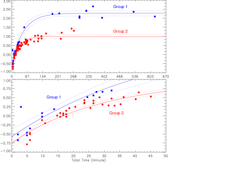
Figure 11: Using the least-squares method, the OPEA models derived from the detected 81 flares. In the upper panel, the filled circles represent the observations, while the continuous lines and dashed lines show the models, and the confidence intervals of 95%, respectively. The part of the figure, where the flares with low energy, are located is re-plotted to show the detail in this part.

Table 6: The parameters obtained from the OPEA models, using the least-squares method.

Parameter	Group1	Group2
$Y_{0}$	$-$0.5732$\pm$0.1013	$-$0.7440$\pm$0.0955
$Plateau$	2.2692$\pm$0.0704	0.9975$\pm$0.0470
$K$	0.00034$\pm$0.00004	0.00056$\pm$0.00006
$\tau$	2926.2	1786.3
Half-time	2028.3	1238.2
Span	2.8425$\pm$0.1175	1.7415$\pm$0.0897
95% Confidence Intervals
$Y_{0}$	$-$0.78324 to -0.36321	$-$0.93572 to -0.55232
$Plateau$	2.1233 to 2.4151	0.90322 to 1.0917
$K$	0.00025 to 0.00043	0.00044 to 0.00068
$\tau$	2316.9 to 3970.3	1462.2 to 2295.0
Half-time	1605.9 to 2752.0	1013.5 to 1590.8
Span	2.5987 to 3.0862	1.5614 to 1.9216
Goodness of Fit
$R^{2}$	0.9682	0.9013
$p-value$ (D’Agostino & Pearson)	0.001	0.008
$p-value$ (Shapiro-Wilk)	0.009	0.009
$p-value$ (Kolmogorov-Smirnov)	0.001	0.001

We test the $OPEA$ models derived for both groups, by using three different methods, the D’Agostino-Pearson normality test, the Shapiro-Wilk normality test and the Kolmogorov-Smirnov test (D’Agostino & Stephens, 1986) to check whether there are any other functions to model the distributions on $\tau_{t}$ - $log~{}P$ plane. In these tests, the probability value ($p-value$) was found to be smaller than 0.001, meaning that there is no other proper function to model the distribution (Motulsky, 2007; Spanier & Oldham, 1987). Considering the correlation coefficient squared ($R^{2}$) values in the Talbe 6, we conclude that the separation of the flares into two groups is statistically real.

In the literature, the distribution of flare cumulative frequency ($\nu(P)$) called as "the flare energy spectrum", which is a frequency serial computed for different flare energy limits for a star, has been derived several decades ago to identify the character of the flare energy (Gershberg, 1972, 2005). The distribution of $\nu(P)$ has been derived by using Equation 6 (Gershberg, 1972).

$$\nu(P)=\int_{P_{min}}^{P_{max}}\nu(P)dP$$ (6)

However, the flare frequencies in the cumulative distribution have been computed for different limits of the flare equivalent durations instead of the flare energy, because of the luminosity term ($L$) in the energy equation of $E=P\times L$. The distribution of flare cumulative frequency is shown in Figure 12 uppermost panel. We searched the best function to fit the distribution of flare cumulative frequency via least-squares method, and find that the most suitable function is an exponential function, which provides correlation coefficient $R^{2}$ higher than 0.90. We test the possibility of any other function, which might provide a better representation, with the methods applied to the OPEA model, and find $p-values$ smaller than 0.001, indicating no alternative function to the exponential function. Figure 12 middle panel shows residuals from the best-fitting exponential functions to the distributions.

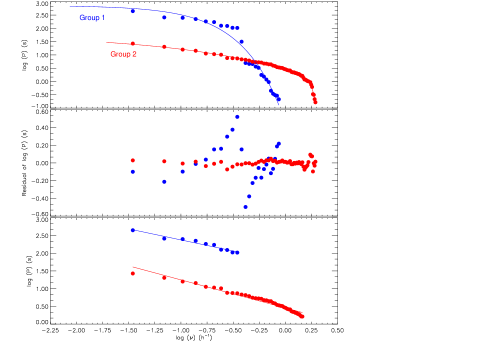
Figure 12: In the upper panel, the flare equivalent duration, $log~{}P$, distribution are plotted versus the flare cumulative frequency on the logarithmic scale for two groups of flares. The filled circles represent computed flare cumulative frequencies, while the lines show the exponential fits. In the middle panel, residuals from the exponential fits are shown. Colours have the same meaning as in the upper panel. In the bottom panel, linear parts of the distributions are plotted. In this panel, linear fits given by Equations 7 and  8 are derived by using the least-squares method.

$$log(P)=-0.6234(\pm 0.0493)\times 1.7510(\pm 0.4238)$$ (7)

$$log(P)=-0.7931(\pm 0.0260)\times 0.4526(\pm 0.0117)$$ (8)

The most important parameter is the slope of the linear fit derived for the linear part of the flare equivalent duration distribution plotted versus the flare cumulative frequency on the logarithmic scale (Gershberg, 2005). In order to find the slopes for two groups, following Gershberg (2005), the distribution were modelled by Equations 7 and 8. In a result, the slope of linear fit of Group 1 flares was found to be -0.6234$\pm$0.0493, while it was found to be -0.7931$\pm$0.0260 in the case of Group 2.

In order to find out where the flares occur on the active component, we derive the orbital phase distribution for all flares. In this respect, using the orbital period and ephemeris time given in Equation 2, we calculate the phase of each flare by considering the time at the moment of the flare. Figure 13 shows the phase distribution of 81 flares, where the flare total number is computed for every 0.05 orbital phase step.

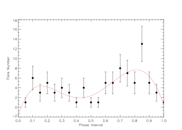
Figure 13: The distribution of flare total number in phase range of 0.05 is plotted with the simple Poisson error for each count versus phase for 81 flares.

Among detected 81 flares, 25 of them belongs to the Group 1, while the remaining 56 flares belong to the Group 2. Ishida et al. (1991) described two frequencies for the stellar flare activity. These frequencies are defined as in Equation 9 and Equation 10,

$$N_{1}=\Sigma n_{f}/\Sigma\tau_{t}$$ (9)

$$N_{2}=\Sigma P/\Sigma\tau_{t}$$ (10)

where $\Sigma n_{f}$ is the total flare number detected in the observations, and $\Sigma\tau_{t}$ is the total observing duration, while $\Sigma P$ is the total equivalent duration obtained from all the flares. We compute both $N_{1}$ and $N_{2}$ flare frequencies for all flares. We carry out the same computation separately for both groups. Table 7 tabulates the computation results.

Table 7: Flare frequencies computed for all flares and grouped flares.

Parameters	All	Group 1	Group 2
Total Time (h)	693.91496	693.91496	693.91496
Flare Number	81	25	56
Total Equivalient Duration (s)	2305.08277	2048.87285	256.20992
$N_{1}$ ($h^{-1}$)	0.11673	0.03603	0.08070
$N_{2}$	0.00092	0.00082	0.00010

4 Discussion and results

Spectroscopic and photometric analysis of KIC 12418816 revealed that the system is a detached binary on a circular orbit. Combined spectroscopic orbit and light curve model parameters lead to the 0.88$\pm$0.06 $M_{\odot}$of mass, 0.85$\pm$0.02 $R_{\odot}$of radius and 4.521$\pm$0.015 of log $g$ for the primary component, while the same parameters are 0.84$\pm$0.05 $M_{\odot}$, 0.84$\pm$0.02 $R_{\odot}$and 4.511$\pm$0.009 for the secondary component. Calculated composite spectrum of the system via 54 Psc + 54 Psc configuration provides very good agreement with the observed composite spectrum of the system. Moreover, we observe strong emission from both components in the core of Ca ii H&K lines, while $H_{\beta}$ and $H_{\alpha}$ lines of both components are in form of filled emission, and almost embedded into the continuum level. These emission features clearly indicate strong chromosperic activity of both components. We also observe the traces of the activity of the components both in the $O-C$ diagram as irregular sinusoidal wave pattern, and in the light curves as frequent flares and light variation at out-of-eclipse. All These findings indicate that the system is composed of two almost twin and very active K0 main sequence stars with a detached configuration, which makes the system unique among its analogues.

The age of the system is given as log(age)=9.53 Gyr by Morton et al. (2016). Plotting the components on $Log~{}T_{eff}-Log~{}L/L_{\odot}$ plane, we find that the components are located close to the Zero Age Main Sequence (ZAMS) rather than the Terminal Age Main Sequence (TAMS), thus indicating that both components must be relatively younger than the age reported in Morton et al. (2016).

The light variation at out-of-eclipse phases indicates an unstable sinusoidal variation with a variable amplitude from one cycle to the next, while $\theta_{min}$ values migrates towards the decreasing phases. Considering the properties of the components, rotational modulation of cool spots is the most possible explanation for the out-of-eclipse variations. However, it is hard to decide which component is actually spotted since both components exhibit emission features in Ca ii H&K, $H_{\beta}$ and $H_{\alpha}$ lines. Assuming that both components possess cool spots on their surface, one would expect a complicated light curve pattern at out-of-eclipse phases, due to the interfering rotational modulations from both components. Furthermore, $\theta_{min}$ values would have a scattered distribution versus time. In the case of KIC 12418816, we observe rather regular patterns at out-of-eclipse phases, which resembles typical light curve of a spotted single star. We observe the similar regularity in the distribution of $\theta_{min}$ values (Figure 9), which smoothly follows a linear trend. These suggest that only one of the component is spotted. Inspecting the strength of emission (Figure 4), one can see that the emission strength of the secondary component in Ca ii H&K, $H_{\beta}$ and $H_{\alpha}$ lines seems generally stronger compared to the primary component, thus the secondary component is possibly the spotted component. In this case, the primary component still exhibits chromospheric activity, but without rotational modulation of spots. We note that both components have flare activity, no matter whether they have spots on their surface. There are several stars exhibiting flare activity without any rotational modulation in their light curves, as in the case of the primary component of KIC 12418816. AD Leo and EQ Peg are such stars, which are well-known UV Ceti type variables (Dal & Evren, 2011b, a).

We investigated migration behaviour of the spotted areas by tracing $\theta_{min}$ values, and find that $\theta_{min}$ values migrates towards decreasing phases as the time progress. Migration between 0.99 and 0.00 phases repeats itself $\sim$6.5 times through the 4 years of $Kepler$ photometry and obviously indicate longitudinal migration of active region on the surface of the active (secondary) component. Applying linear fit to the adjusted $\theta_{min}$ values, we find the migration period of the active region as 0.72$\pm$0.05 year. This period is similar to the solar analogue stars. Using the orbital period and the migration period of KIC 12418816, one can find mean rotation period of the spotted component, as described by Hall & Busby (1990), and estimate the surface share via the difference between the mean rotation period and the orbital period. We find the mean rotation period as $1.51\pm 0.21$ day, which leads to the surface share $\Delta\Omega=0.02\pm 0.87$ rad day^-1. Since the statistical uncertainty is very large compared to the shear value, we refrain further discussion on the surface shear.

Another remarkable spot activity property of KIC 12418816 comes from the $\theta_{min}$ shift versus time. The residual of $\theta_{min}$ shift obtained after the linear correction exhibits a systematic sinusoidal variation, in which there is also a quasi-periodic wave like second variation with smaller amplitude. The systematic sinusoidal variation with larger amplitude should be caused by globally swinging position of spotted area due to differential rotation on the stellar surface. However, the quasi-periodic wave like second variation with smaller amplitude should be affected by local spots which rapidly evolve on the stellar surface. Figure 8 panel $b$ provides clear evidence of such a rapid spot evolution, and migration.

Apart from the spot activity, the most notable variation is flare activity at out-of-eclipses. After determining flare parameters of 81 detected flares, we modelled the distribution of flare equivalent durations on the logarithmic scale versus the flare total time with the OPEA model (Equation 5). The initial attempts did not give any statistically acceptable model for the distribution due to large scattering. The similar phenomenon is seen in the flare study of Kamil & Dal (2017). Considering both $R^{2}$ and the $p-values$ derived for the model, they modelled the flare equivalent duration data with two different OPEA models. Following the way they defined, we modelled the flare equivalent duration data with two different OPEA models in this study. We found plateau value as 2.2692$\pm$0.0704 s from the model of Group 1 flares, while it was computed as 0.9975$\pm$0.0470 s from the model of Group 2. The plateau value of first group is 2 times larger than that found from Group 2.

The main average of the equivalent durations in the logarithmic scale for the plateau flares of Group 1 was found to be 2.253$\pm$0.064 s with standard deviation of 0.203 s, and it was found to be 1.020$\pm$0.065 s with standard deviation of 0.222 s for Group 2. The results confirm that these two groups are statistically different from each other.

In this point, one may claim that the separation is caused due to the flare morphology (Moffett, 1974; Dal & Evren, 2010b; Hawley et al., 2014a; Davenport et al., 2014a). For example, one can claim that slow flares are aggregated in Group 2, while the fast flares are aggregated in Group 1. In fact, according to Dal & Evren (2010b); Hawley et al. (2014a); Davenport et al. (2014a), a slow flare has lower energy than a fast flare with same duration. Therefore, this situation can explain the 2 times difference between these two groups. To test whether there is any morphological affect, the light variations of all flares were morphologically checked, and we see that both groups have both flare morphologies.

However, according to Dal & Evren (2010a, 2011b), the plateau value is defined as a saturation level of white-light flares for a star, and also a star can have just one plateau values depending on its $B-V$ color index. Thus, if the plateau values are markedly different for two group flares, it means that these flare groups come from two different stars, whose $B-V$ color indexes are different from each other. Dal (2012) showed that the plateau values systematically vary depending on the $B-V$ colours. In this case, the flares compiled as Group 1 and Group 2 in this study must come from two different sources. The magnetic activity sensitive lines of both two components exhibit strong emission. These two results confirm each other, i.e. according to spectral data, both components have high level magnetic activity, therefore both of them must exhibit flare activity.

In the literature, there is no relation between flare saturation level and existence of stellar cool spot activity. For instance, in the case of KOI-256, one of the interesting binary system observed by $Kepler$ Satellite, the plateau value was found to be 2.3121$\pm$0.0964 s (Yoldaş & Dal, 2017). In the case of FL Lyr, it was found to be 1.232$\pm$0.069 s (Yoldaş & Dal, 2016). The flares compiled as Group 1 in this study behave as the same as flares detected from KOI-256, while Group 2 flares behave as the same as flares detected from FL Lyr. Yoldaş & Dal (2016, 2017) revealed that both KOI-256 and FL Lyr have high level spot activity on their surfaces. Comparing these samples, one expects that both components of KIC 12418816 could exhibit spot activity depending on their plateau values. However, our findings above indicate that just one of the component possesses spotted areas on its surface. A similar case has been described by Kamil & Dal (2017) for KIC 2557430. In the case of KIC 2557430, although there are two sources exhibiting flares with different plateau levels, only one of them exhibits stellar spot activity.

The mostly discussed model and parameter in the literature are the cumulative flare frequency distribution and the slope of its linear fit (Gershberg, 1972; Lacy et al., 1976; Walker, 1981; Gershberg & Shakhovskaia, 1983; Pettersen et al., 1984; Mavridis & Avgoloupis, 1986; Gershberg, 2005; Hawley et al., 2014b; Davenport et al., 2014b). In this study, the cumulative flare frequency distributions were derived for the flares in both groups. Modelling the distributions by Equations 7 and 8, the linear fits were derived. The slope of linear fit of Group 1 flares was computed as -0.6234$\pm$0.0493, while it was computed as $-$0.7931$\pm$0.0260 for Group 2 flares.

Besides the plateau value, there is one more indicator for the flare activity level of stars. (Ishida et al., 1991) described $N_{1}$ flare frequencies. $N_{1}$ flare frequency given by Equation 9 is the flare number per hour, while $N_{2}$ flare frequency given by Equation 10 is the flare total equivalent duration emitting per hour. We find $N_{1}$ as 0.03603 $h^{-1}$ for flares of Group 1 and 0.08070 $h^{-1}$ for Group 2. It means that the Group 2 flares are more frequent than Group 1 flares. However, as it is seen from $N_{2}$ flare frequencies listed in Table 7, the flares of Group 1 are more powerful than those of Group 2. In a result, Group 1 flares are rare but powerful, while Group 2 flare are less powerful compared to the Group 1 flares but more frequent.

In general, an unexpected result comes from the orbital phase distribution of flares. Unlike what is known and discussed in the literature (Hawley et al., 2014b), the flare number seems to be rising around the phases of 0.15 and 0.85 (Figure 13). It means that one can observe the flares more frequently just before and just after the primary eclipse of the whole light curve. This is very impressive because it indicates some clue about magnetic interaction between the components. Owing to the orbital properties of the system, The components are close enough to each other to get an interaction easily when a flare occurs on surface of a component. The situation makes the system an interesting binary to study for the readers working on magnetic natures of binaries in different evolutionary stages.

References

- Armstrong et al. (2014) Armstrong D. J., Gómez Maqueo Chew Y., Faedi F., Pollacco D., 2014, MNRAS, 437, 3473
- Balaji et al. (2015) Balaji B., Croll B., Levine A. M., Rappaport S., 2015, MNRAS, 448, 429
- Benz (2008) Benz A. O., 2008, Living Reviews in Solar Physics , 5, 1
- Benz & Güdel (2010) Benz A. O., Güdel M., 2010, ARA&A, 48, 241
- Berdyugina & Järvinen (2005) Berdyugina S. V., Järvinen S. P., 2005, Astronomische Nachrichten , 326, 283
- Berdyugina & Usoskin (2003) Berdyugina S. V., Usoskin I. G., 2003, A&A, 405, 1121
- Bogart (1982) Bogart R. S., 1982, Sol. Phys., 76, 155
- Carrington (1859) Carrington R. C., 1859, MNRAS, 20, 13
- Coughlin et al. (2011) Coughlin J. L., López-Morales M., Harrison T. E., Ule N., Hoffman D. I., 2011, AJ, 141, 78
- D’Agostino & Stephens (1986) D’Agostino R. B., Stephens M. A., 1986, Goodness-of-fit techniques
- Dal (2012) Dal H. A., 2012, PASJ, 64, 82
- Dal & Evren (2010a) Dal H. A., Evren S., 2010a, AJ, 140, 483
- Dal & Evren (2010b) Dal H. A., Evren S., 2010b, AJ, 140, 483
- Dal & Evren (2011a) Dal H. A., Evren S., 2011a, PASJ, 63, 427
- Dal & Evren (2011b) Dal H. A., Evren S., 2011b, AJ, 141, 33
- Davenport et al. (2014a) Davenport J. R. A., et al., 2014a, ApJ, 797, 122
- Davenport et al. (2014b) Davenport J. R. A., et al., 2014b, ApJ, 797, 122
- Dawson & Trapp (2004) Dawson B., Trapp R., 2004, Basic & Clinical Biostatistics 4/E (EBOOK). LANGE Basic Science, McGraw-Hill Education, https://books.google.com.tr/books?id=p6hu-qU2zpsC
- Foreman-Mackey et al. (2013) Foreman-Mackey D., Hogg D. W., Lang D., Goodman J., 2013, PASP, 125, 306
- Frasca et al. (2009) Frasca A., Covino E., Spezzi L., Alcalá J. M., Marilli E., Fżrész G., Gandolfi D., 2009, A&A, 508, 1313
- Gershberg (1972) Gershberg R. E., 1972, Ap&SS, 19, 75
- Gershberg (2005) Gershberg R. E., 2005, Solar-Type Activity in Main-Sequence Stars, 10.1007/3-540-28243-2.
- Gershberg & Shakhovskaia (1983) Gershberg R. E., Shakhovskaia N. I., 1983, Ap&SS, 95, 235
- Gray (2005) Gray D. F., 2005, The Observation and Analysis of Stellar Photospheres
- Gray et al. (2003) Gray R. O., Corbally C. J., Garrison R. F., McFadden M. T., Robinson P. E., 2003, AJ, 126, 2048
- Gray et al. (2006) Gray R. O., Corbally C. J., Garrison R. F., McFadden M. T., Bubar E. J., McGahee C. E., O’Donoghue A. A., Knox E. R., 2006, AJ, 132, 161
- Green et al. (1996) Green S. B., Salkind N. J., Jones T. M., 1996, Using SPSS for Windows; Analyzing and Understanding Data, 1st edn. Prentice Hall PTR, Upper Saddle River, NJ, USA
- Haisch et al. (1991) Haisch B., Strong K. T., Rodono M., 1991, ARA&A, 29, 275
- Hall & Busby (1990) Hall D. S., Busby M. R., 1990, in NATO Advanced Science Institutes (ASI) Series C. p. 377
- Hawley et al. (2014a) Hawley S. L., Davenport J. R. A., Kowalski A. F., Wisniewski J. P., Hebb L., Deitrick R., Hilton E. J., 2014a, ApJ, 797, 121
- Hawley et al. (2014b) Hawley S. L., Davenport J. R. A., Kowalski A. F., Wisniewski J. P., Hebb L., Deitrick R., Hilton E. J., 2014b, ApJ, 797, 121
- Hodgson (1859) Hodgson R., 1859, MNRAS, 20, 15
- Huber et al. (2014) Huber D., et al., 2014, ApJS, 211, 2
- Hudson & Khan (1996) Hudson H. S., Khan J. I., 1996, in Bentley R. D., Mariska J. T., eds, Astronomical Society of the Pacific Conference Series Vol. 111, Astronomical Society of the Pacific Conference Series. pp 135–144
- Ibanoǧlu et al. (2006) Ibanoǧlu C., Soydugan F., Soydugan E., Dervişoǧlu A., 2006, MNRAS, 373, 435
- Ishida et al. (1991) Ishida K., Ichimura K., Shimizu Y., Mahasenaputra 1991, Ap&SS, 182, 227
- Kamil & Dal (2017) Kamil C., Dal H. A., 2017, Publ. Astron. Soc. Australia, 34, e029
- Klinglesmith & Sobieski (1970) Klinglesmith D. A., Sobieski S., 1970, AJ, 75, 175
- Kowalski et al. (2013) Kowalski A. F., Hawley S. L., Wisniewski J. P., Osten R. A., Hilton E. J., Holtzman J. A., Schmidt S. J., Davenport J. R. A., 2013, ApJS, 207, 15
- Kron (1952) Kron G. E., 1952, ApJ, 115, 301
- Kunkel (1975) Kunkel W. E., 1975, in Sherwood V. E., Plaut L., eds, IAU Symposium Vol. 67, Variable Stars and Stellar Evolution. pp 15–46
- Lacy et al. (1976) Lacy C. H., Moffett T. J., Evans D. S., 1976, ApJS, 30, 85
- Levenberg (1944) Levenberg K., 1944, Quaterly Journal on Applied Mathematics, pp 164–168
- Lopez Arroyo (1961) Lopez Arroyo M., 1961, The Observatory, 81, 205
- Marcy & Chen (1992) Marcy G. W., Chen G. H., 1992, ApJ, 390, 550
- Marquardt (1963) Marquardt D. W., 1963, Journal of the Society for Industrial and Applied Mathematics, 11, 431
- Mavridis & Avgoloupis (1986) Mavridis L. N., Avgoloupis S., 1986, A&A, 154, 171
- Mirzoian (1990) Mirzoian L. V., 1990, in Mirzoian L. V., Pettersen B. R., Tsvetkov M. K., eds, IAU Symposium Vol. 137, Flare Stars in Star Clusters, Associations and the Solar Vicinity. pp 1–12
- Moffett (1974) Moffett T. J., 1974, ApJS, 29, 1
- Monet (1998) Monet D. G., 1998, in American Astronomical Society Meeting Abstracts. p. 1427
- Morton et al. (2016) Morton T. D., Bryson S. T., Coughlin J. L., Rowe J. F., Ravichandran G., Petigura E. A., Haas M. R., Batalha N. M., 2016, ApJ, 822, 86
- Motulsky (2007) Motulsky H., 2007, GraphPad Software, 31, 39
- Pettersen (1991) Pettersen B. R., 1991, Mem. Soc. Astron. Italiana, 62, 217
- Pettersen et al. (1984) Pettersen B. R., Coleman L. A., Evans D. S., 1984, ApJS, 54, 375
- Pigatto (1990) Pigatto L., 1990, in Mirzoian L. V., Pettersen B. R., Tsvetkov M. K., eds, IAU Symposium Vol. 137, Flare Stars in Star Clusters, Associations and the Solar Vicinity. pp 117–120
- Pinsonneault et al. (2012) Pinsonneault M. H., An D., Molenda-Żakowicz J., Chaplin W. J., Metcalfe T. S., Bruntt H., 2012, ApJS, 199, 30
- Pols et al. (1998) Pols O. R., Schröder K.-P., Hurley J. R., Tout C. A., Eggleton P. P., 1998, MNRAS, 298, 525
- Prša et al. (2011) Prša A., et al., 2011, AJ, 141, 83
- Rodono (1986) Rodono M., 1986, NASA Special Publication, 492
- Skumanich (1972) Skumanich A., 1972, ApJ, 171, 565
- Slawson et al. (2011) Slawson R. W., et al., 2011, AJ, 142, 160
- Spanier & Oldham (1987) Spanier J., Oldham K. B., 1987, An Atlas of Functions. Taylor & Francis/Hemisphere, Bristol, PA, USA
- Stanek (1972) Stanek W., 1972, Sol. Phys., 27, 89
- Stauffer (1991) Stauffer J. R., 1991, in Catalano S., Stauffer J. R., eds, NATO Advanced Science Institutes (ASI) Series C Vol. 340, NATO Advanced Science Institutes (ASI) Series C. p. 117
- Tonry & Davis (1979) Tonry J., Davis M., 1979, AJ, 84, 1511
- Tran et al. (2013) Tran K., Levine A., Rappaport S., Borkovits T., Csizmadia S., Kalomeni B., 2013, ApJ, 774, 81
- Walker (1981) Walker A. R., 1981, MNRAS, 195, 1029
- Wall & Jenkins (2003) Wall J. V., Jenkins C. R., 2003, Practical Statistics for Astronomers
- Watson (2006) Watson C. L., 2006, Society for Astronomical Sciences Annual Symposium, 25, 47
- Wilson & Devinney (1971) Wilson R. E., Devinney E. J., 1971, ApJ, 166, 605
- Wilson & Van Hamme (2014) Wilson R. E., Van Hamme W., 2014, ApJ, 780, 151
- Yoldaş & Dal (2016) Yoldaş E., Dal H. A., 2016, Publ. Astron. Soc. Australia, 33, e016
- Yoldaş & Dal (2017) Yoldaş E., Dal H. A., 2017, Publ. Astron. Soc. Australia, in press
- Zacharias et al. (2004) Zacharias N., Monet D. G., Levine S. E., Urban S. E., Gaume R., Wycoff G. L., 2004, in American Astronomical Society Meeting Abstracts. p. 1418
- van Hamme (1993) van Hamme W., 1993, AJ, 106, 2096