Solution of n-⁴He elastic scattering problem using Faddeev-Yakubovsky equations

Abstract

The first ever numerical solution of five-body Faddeev-Yakubovsky equations is presented in this work. Modern realistic Nucleon-Nucleon Hamiltonians have been tested when describing low energy elastic neutron scattering on ⁴He nucleus. Obtained results have been compared with those available in the literature and based on solution of the Schrödinger equation.

Solution of nuclear bound state problem by ab-initio methods have reached new heights during the last decade Pieper et al. (2002); Hagen et al. (2010); Barrett et al. (2013); Tsukiyama et al. (2011); Somà et al. (2013). Accurate description of the nuclei composed of several nucleons has been made possible. However bound-state properties, such as binding energies, nuclear densities and radii, provide only a rather restricted set of data with which to test our understanding of the nuclear force. It is the nuclear scattering experiment, where cross sections can be measured as a function of energy, reaction channel, angular distributions, and polarization phenomena, provides the richest set of data on nuclear interaction and dynamics.

However description of a few-nucleon scattering problem in its full complexity turns to be quite problematic. The main difficulty is related with the fact that unlike bound-state wave function, which asymptotically approaches zero for large values of any two-particle separation, the scattering wave function is not-compact. When solving a scattering problem in configuration space proper treatment of boundary conditions is required, which in a Lippmann-Schwinger equation formulation of the scattering problem are ill defined. In early 60’s Faddeev formulated the t-matrix approach to the three-body problem Faddeev (1961), providing a proper way to formulate boundary conditions for continuum problems dominated by the short-ranged interactions. Just a few years later Faddeev’s revolutionary work has been generalized to any number of particles by Yakubovsky Yakubovsky (1967). Regardless these revolutionary mathematical developments progress in solution of Faddeev-Yakubovsky equations (FYe) is slow and for long years was limited to A=3 and A=4 cases Glöckle et al. (1996); Viviani et al. (2017). The main difficulty is related to the complexity of these equations. Indeed in Faddeev-Yakubovsky (FY) approach a few-particle Schrödinger equation is transformed into a set of differential equations for so called FY components, which are introduced with a purpose to uncouple asymptotes of the binary scattering channels. The number of these components (channels) increases like a factorial of a particle number, resulting into very poor scaling of FY formalism with a particle number.

One should mention that FY equations is not an unique way to solve scattering problem in configuration space. Diverse scattering problems may be solved accurately also based on the Schrödinger equation, if the Faddeev decomposition (or its equivalent) is used in order to enforce the proper boundary conditions Viviani et al. (1998). Furthermore, due to poor scaling of FYe’s with a particle number, approaches based on Schrödinger equation, like Navrátil et al. (2010), have much brighter prospects than FY approach in describing systems containing more than five particles. However once addressing scattering problem with a Schrödinger equation one should be cautious about the possibility to end up with the spurious solutions. Therefore if computationally accessible, due to their mathematically rigorous nature FYe formalism remains a reference in solving few-particle scattering problem.

In this study the first solution of FYe in configuration space is presented for a five-body system. Modern realistic Nucleon-Nucleon interactions will be employed to describe neutron elastic scattering on ⁴He nucleus. Results will be compared with those available in the literature and obtained using methods based on solving Schrödinger equation.

Calculations have been performed for three significantly different realistic nucleon-nucleon interaction models. The considered potentials describe very accurately NN scattering data and include the tail parts determined by the pion-exchange between the nucleons. Nevertheless these models differ significantly in the procedure adapted to parameterize their short range parts. The AV18 model is a local NN potential Wiringa et al. (1995); INOY04 model contains strongly non-local core within R=2 fm range for S and P waves Doleschall (2004); whereas I-N3LO potential Entem and Machleidt (2003) is non-local in momentum space and is based on the $\chi$EFT approach, being derived up to next-to-next-to-next-to-leading order in chiral perturbation theory. All the results presented in what follows have been obtained considering equal masses for neutrons and protons ($m_{n}=m_{p}=m$) with ${\frac{\hbar^{2}}{m}}=41.471$ MeV fm².

I Formalism

II 5-body FY equations

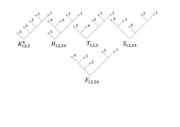
Figure 1: (Color online) 5-particle Jacobi coordinate sets used to describe FY components, denoted in this work as $K,T,H,S,F$.

In the late sixties Yakubovsky demonstrated a scheme how to generalize 3-body Faddeev equations to N-body system of particles governed by short-ranged interactions Yakubovsky (1967). A detailed derivation of 5-body FY equations has been performed in ref. Sasakawa (1977). Derivations of N-body FY equations starts by decomposing systems total wave function into binary partitions, similar to 3-body Faddeev components:

$$\phi_{ij}=G_{0}V_{ij}\Psi.$$ (1)

For a five body system one may construct 10 different binary components by permuting particle indexes $(ij)$. In that follows I will denote by letters $(ijklm)$ combination of particle indexes $(12345)$. It is easy to verify that the total systems wave function is recovered by simply adding binary components:

$$\Psi(x,y,z,w)=\sum\limits_{i<j}^{5}\phi_{ij}(x,y,z,w).$$ (2)

The binary components $\phi_{ij}(x,y,z,w)$ are further split into four-body type components by following a pattern of breaking five body $(ijklm)$ partition into clusters and their subclusters. One has two types of four-body components, which are similar to ones appearing in four-body FY equations:

$$\left\{\begin{array}[]{c}\psi_{ij}^{ijk}=G_{ij}V_{ij}(\phi_{jk}+\phi_{ki}),\\ \psi_{ij}^{ij,kl}=G_{ij}V_{ij}\phi_{kl}.\end{array}\right.$$ (3)

Here 5-body Green’s $G_{ij}$ includes single interaction term $V_{ij}$, i.e. $G_{ij}=(E-H_{0}-V_{ij})^{-1}$. For a 5-body system there exist 30 different 4-body components of type $\psi_{ij}^{ijk}$ as well as 30 components of type $\psi_{ij}^{ij,kl}$. Using Yakubovsky’s scheme one may easily decompose the binary components into the 4-body ones:

$$\phi_{ij}=\psi_{ij}^{ijk}+\psi_{ij}^{ijl}+\psi_{ij}^{ijm}+\psi_{ij}^{ij,kl}+\psi_{ij}^{ij,km}+\psi_{ij}^{ij,lm}.$$ (4)

Finally, the four-body components are decomposed into a sum of 5-body FY components:

$$\left\{\begin{array}[]{cc}\psi_{ij}^{ijk}=K_{ij,k}^{l}+K_{ij,k}^{m}+\mathcal{T}_{ij,k}&\text{(30 amplitudes)},\\ \psi_{ij}^{ij,kl}=H_{ij,kl}+\mathcal{S}_{ij,kl}+\mathcal{F}_{ij,kl}&\text{(30 amplitudes)}.\end{array}\right.$$ (5)

Faddeev-Yakubovsky equations involve five different types of 5-body FY components (see Fig.1), denoted in this work by $K_{ij,k}^{l},T_{ij,k,}H_{ij,kl},S_{ij,kl}$ and $\mathcal{F}_{ij,kl}$. In total, there exist 60 components of type-K and 30 components for each of the types $H,S,T$ and $\mathcal{F}$. 5-body FY equations constitutes a set of 180 coupled equations, each of which might be associated with a particular FY component. One has 5 non-trivial equations, each highlighting one particular component of different type. By separating terms associated with a highlighted component in the right hand side of the relations – these equations can be summarized as follows:

$$(E-\widehat{H}_{0}-V_{12})K_{12,3}^{4} = V_{12}(K_{13,2}^{4}+K_{23,1}^{4}+K_{13,4}^{5}+K_{23,4}^{5}+K_{13,4}^{2}+K_{23,4}^{1}$$

$$+\mathcal{T}_{13,4}+\mathcal{T}_{23,4}$$

$$+H_{13,24}+H_{23,14}+\mathcal{S}_{13,24}+\mathcal{S}_{23,14}+\mathcal{F}_{13,24}+\mathcal{F}_{23,14}),$$

$$(E-\widehat{H}_{0}-V_{12})H_{12,34} = V_{12}(H_{34,12}$$

$$+K_{34,1}^{2}+K_{34,2}^{1}+K_{34,1}^{5}+K_{34,2}^{5}$$

$$+\mathcal{T}_{34,1}+\mathcal{T}_{34,2}),$$

$$(E-\widehat{H}_{0}-V_{12})\mathcal{T}_{12,3} = V_{12}(\mathcal{T}_{13,2}+\mathcal{T}_{23,1}$$

$$+H_{13,45}+H_{23,45}$$

$$+\mathcal{S}_{13,45}+\mathcal{S}_{23,45}$$

$$+\mathcal{F}_{13,45}+\mathcal{F}_{23,45}),$$

$$(E-\widehat{H}_{0}-V_{12})\mathcal{S}_{12,34} = V_{12}(\mathcal{F}_{34,12}+\mathcal{S}_{34,15}+\mathcal{S}_{34,25}$$

$$+\mathcal{F}_{34,15}+\mathcal{F}_{34,25}$$

$$+H_{34,15}+H_{34,25}),$$

$$(E-\widehat{H}_{0}-V_{12})\mathcal{F}_{12,34} = V_{12}(\mathcal{S}_{34,12}$$

$$+K_{34,5}^{1}+K_{34,5}^{2}$$

$$+\mathcal{T}_{34,5}).$$

Other equations follow from this set by simply permuting particle indexes in the ordered way. For a system of five identical particles one can reduce the problem to solving only one set of the five equations, since there remains only five independent FY components ($K_{ij,k}^{l},T_{ij,k,}H_{ij,kl},S_{ij,kl}$ and $\mathcal{F}_{ij,kl}$). Other components may be obtained from a selected set of components ($K,H,S,T,\mathcal{F}$) by using particle-permutation symmetry relations.

III Coordinates

Each FY component $F=(K,T,H,S,\mathcal{F})$ is a function in twelve-dimensional configuration space, determined by the four 3D vectors ($\vec{x},\vec{y},\vec{z},\vec{w}$). It is convenient to express the FYCs in their proper set of Jacobi coordinates, see Fig. 1. Jacobi coordinate connecting two clusters $\left(s\right)$ and $\left(t\right)$ are expressed using a general formulae:

$$(\overrightarrow{x},\overrightarrow{y},\overrightarrow{z},\overrightarrow{w})=\sqrt{\frac{2m_{s}m_{t}}{m(m_{s}+m_{t})}}\left(\overrightarrow{r}_{s}-\overrightarrow{r}_{t}\right),$$ (7)

where $m_{s}$ and $m_{t}$ are the masses of the clusters, while $\overrightarrow{r}_{s}$ and $\overrightarrow{r}_{t}$ are respective positions of their center-of-masses. A mass factor $m$ of free choice is introduced into the former expression in order to retain the proper units of the distances. When studying systems of identical particles it is convenient to identify this mass with the mass of a single particle (in this study mass of a nucleon). In terms of Jacobi coordinates center-of-mass free Hamiltonian is expressed:

$$H_{0}=-\frac{\hbar^{2}}{m}\left(\Delta_{x}+\Delta_{y}+\Delta_{z}+\Delta_{w}\right).$$ (8)

When studying low energy processes partial wave expansion turns to be a very efficient tool to express angular dependence of the systems wave function. Without exception in this work partial wave expansion is used to describe spatial dependence of FY components as well as their dependence on spin and isospin quantum numbers:

$$F^{JM}(\overrightarrow{x},\overrightarrow{y},\overrightarrow{z},\overrightarrow{w})=\sum\frac{f_{\alpha}(x,y,z,w)}{xyzw}\left|\left\{\left\{l_{x}l_{y}\right\}_{l_{xy}}\left\{l_{z}l_{w}\right\}_{l_{zw}}\right\}_{L}\left\{S\right\}\right\rangle_{JM}\left\{T\right\}_{TT_{z}},$$ (9)

here $\alpha\equiv(l_{x},l_{y},l_{z},l_{w},l_{xy},l_{zw},L,\left\{S\right\},\left\{T\right\})$ is an index representing set of intermediate quantum numbers, coupled to total angular momentum $J$ and total isospin $T$ with its projection $T_{z}$ (for a n-⁴He scattering considered in this work, total isospin and its projection are fixed to T=1/2 and T_z=1/2^-. In the last expression $\left\{S\right\}$ and $\left\{T\right\}$ represent respectively partial-wave basis dependence on spin and isospin, which is provided by:

$$\left\{S\right\}=\left|\left\{\left\{s_{1}s_{2}\right\}_{s_{x}}\left\{s_{3}s_{4}\right\}_{s_{y}}\right\}_{s_{xy}}s_{5}\right\rangle_{SS_{Z}},$$ (10)

here $s_{1}$ to $s_{5}$ are spins of individual nucleons, whereas $s_{x},s_{y},s_{xy},S$ represent quantum numbers of intermediate couplings. An equivalent expression is used to develop isospin dependence $\left\{T\right\}$ of FY components. The reduced components $f_{\alpha}(x,y,z,w)$ represent dependence on radial parts of the coordinates. This dependence is expressed using Lagrange-Laguerre basis functions.

The last set of equations (9-10) define the principal partial-wave basis set employed in this work. However, in parallel, two additional equivalent partial wave coupling schemes have been used. One exposing coupling of angular momenta $\left\{l_{y}l_{z}\right\}_{l_{yz}}$, required in order to perform some permutation operations in yz-space, another explicitly exposing two-particle angular momentum $\left\{l_{x}(s_{1},s_{2})_{s_{x}}\right\}_{j_{x}}$ used to evaluate matrix elements of NN-interaction between particles 1 and 2.

IV Operators

In order to solve FY equations it is useful to define a set of operators, which allow to couple different FY components. First, I introduce a group of operators which couple FY components of different type, but which share the same particle ordering:

$$K_{12,3}^{4} = \left(P^{KH}\right)_{yz}^{1}H_{12,34};\quad H_{12,34}=\left(P^{HK}\right)_{yz}^{1}K_{12,3}^{4},$$

$$K_{12,3}^{4} = \left(P^{KT}\right)_{zw}^{1}\mathcal{T}_{12,3};\quad\mathcal{T}_{12,3}=\left(P^{TK}\right)_{zw}^{1}K_{12,3}^{4},\quad$$

$$H_{12,34} = \left(P^{HS}\right)_{zw}^{1}\mathcal{S}_{12,34};\quad\mathcal{S}_{12,34}=\left(P^{SH}\right)_{zw}^{1}H_{12,34},$$

$$H_{12,34} = \left(P^{HF}\right)_{zw}^{1}\mathcal{F}_{12,34};\quad\mathcal{F}_{12,34}=\left(P^{FH}\right)_{zw}^{1}H_{12,34},$$ (11)

$$\mathcal{S}_{12,34} = \left(P^{SF}\right)_{zw}^{1}\mathcal{F}_{12,34};\quad\mathcal{F}_{12,34}=\left(P^{FS}\right)_{zw}^{1}\mathcal{S}_{12,34},$$

$$\mathcal{T}_{12,3} = \left(\underline{P}^{TS}\right)_{yz}^{0}\mathcal{S}_{12,45};\quad\mathcal{S}_{12,34}=\left(\underline{P}^{ST}\right)_{yz}^{0}\mathcal{T}_{12,5},$$

$$\mathcal{S}_{34,12} = \left(\underline{P}^{SF}\right)_{xy}^{0}\mathcal{F}_{12,34};\quad\mathcal{F}_{34,12}=\left(\underline{P}^{FS}\right)_{xy}^{0}\mathcal{S}_{12,34}.$$

Operators presented on each line represent inverse to each other, i.e. as example $\left(\left(P^{HK}\right)_{yz}^{1}\right)^{-1}=\left(P^{HK}\right)_{yz}^{1}$. Expressions of these operators splits in to tensor product of operators acting in coordinate, spin and isospin spaces. When matrix elements of these operators are properly ordered inverse operator is directly obtained from the original operator by simply permuting its matrix elements and thus does not require separate evaluation or storage.

Second group of operators is used to change the particle ordering:

$$K_{12,3}^{4} = \left(P^{+}\right)_{xy}^{1}K_{23,1}^{4};\quad K_{12,3}^{4}=\left(P^{-}\right)_{xy}^{1}K_{31,2}^{4},$$

$$\mathcal{T}_{12,3} = \left(P^{+}\right)_{xy}^{1}\mathcal{T}_{23,1};\quad\mathcal{T}_{12,3}=\left(P^{-}\right)_{xy}^{1}\mathcal{T}_{31,2},$$ (12)

$$K_{12,3}^{4} = \left(\varepsilon P^{34}\right)_{yz}^{1}K_{12,4}^{3},$$

$$K_{12,3}^{5} = \left(\varepsilon P^{45}\right)_{zw}^{1}K_{12,3}^{5},$$

$$H_{12,34} = \left(P^{H}\right)_{xy}^{0}H_{34,12},$$

$$\left(\widetilde{P}^{3}\right)_{xy}^{1} = \left(P^{+}\right)_{xy}^{1}+\left(P^{-}\right)_{xy}^{1},$$

$$\left(\widetilde{P}^{4}\right)_{yz}^{1} = \left(\varepsilon P^{34}\right)_{yz}^{1};\ \quad\left(\widetilde{P}^{5}\right)_{zw}^{1}=\left(\varepsilon P^{45}\right)_{zw}^{1}.$$

In these expressions operators have been denoted using the general notation $\left(P^{A}\right)_{xy}^{n}$, where integer $n$ indicates number of angular integrations involved in coupling partial amplitudes; $xy$- denotes that this operator transforms radial dependencies of the amplitude in coordinates $x$ and $y$. Expressions for these operators are quite trivial, equivalent to ones used in solving 3-body or 4-body FY equations. Nevertheless their expressions become quite voluminous and will be published elsewhere. When applied successively, this set of operators is sufficient to couple any two FY components and thus solve 5-body FY equations as formulated in eq.(II). Using these definitions 5-body FY equations read:

$$K_{12,3}^{4} = G_{12}V_{12}\left(\widetilde{P}^{3}\right)_{xy}^{1}\left(K_{12,3}^{4}+\left(P^{KH}\right)_{yz}^{1}\left[H_{12,34}+\left(P^{HS}\right)_{zw}^{1}\mathcal{S}_{12,34}+\left(P^{HF}\right)_{zw}^{1}\mathcal{F}_{12,34}\right]\right.,$$ (13)

$$\left.+\left(\widetilde{P}^{4}\right)_{yz}^{1}\left[K_{12,3}^{4}+\left(\widetilde{P}^{5}\right)_{zw}^{1}K_{12,3}^{4}+\left(P^{KT}\right)_{zw}^{1}\mathcal{T}_{12,3}\right]\right),$$

$$H_{12,34} = G_{12}V_{12}\left(\underline{P}^{H}\right)_{xy}^{0}\left(H_{12,34}+2\left(P^{HK}\right)_{yz}^{1}\left[K_{12,3}^{4}+\left(\widetilde{P}^{5}\right)_{zw}^{1}K_{12,3}^{4}+\left(P^{KT}\right)_{zw}^{1}\mathcal{T}_{12,3}\right]\right),$$

$$\mathcal{T}_{12,3} = G_{12}V_{12}\left(\widetilde{P}^{3}\right)_{xy}^{1}\left(\mathcal{T}_{12,3}+\left(\underline{P}^{TS}\right)_{yz}^{0}\left[\mathcal{S}_{12,34}+\left(P^{SF}\right)_{zw}^{1}\mathcal{F}_{12,34}+\left(P^{SH}\right)_{zw}^{1}H_{12,34}\right]\right),$$

$$\mathcal{S}_{12,34} = G_{12}V_{12}\left(\left(\underline{P}^{ST}\right)_{yz}^{0}\left(\widetilde{P}^{3}\right)_{xy}^{1}\left(\underline{P}^{TS}\right)_{yz}^{0}\left(\underline{P}^{SF}\right)_{xy}^{0}\left[\mathcal{F}_{12,34}+\left(P^{FH}\right)_{zw}^{1}H_{12,34}+\left(P^{FS}\right)_{zw}^{1}\mathcal{S}_{12,34}\right]\right.,$$

$$+\left.\left(\underline{P}^{SF}\right)_{xy}^{0}\mathcal{F}_{12,34}\right),$$

$$\mathcal{F}_{12,34} = G_{12}V_{12}\left(\underline{P}^{FS}\right)_{xy}^{0}\left[\mathcal{F}_{12,34}+\left(\underline{P}^{ST}\right)_{yz}^{0}\left(\mathcal{T}_{12,3}+2\left(P^{TK}\right)_{zw}^{1}K_{12,3}^{4}\right)\right].$$

Since in this work a system of five formally identical particles is considered, the last set of equations is written for the components, where particles are ordered in a natural succession (12345).

The last set of equations is sufficient to solve 5-body problem and obtain to this problem related physical observables – binding energies or phaseshifts. However in order to estimate expectations values of the physical operators one may require to reproduce total systems wave function, which may be expressed in terms of FY components:

$$\Psi(x,y,z,w) = \sum\limits_{i<j}^{5}\phi_{ij}(x,y,z,w)$$

$$\phi_{12} = \psi_{12}^{123}+\psi_{12}^{124}+\psi_{12}^{125}+\psi_{12}^{12,34}+\psi_{12}^{12,35}+\psi_{12}^{12,45}$$

$$= \left[1+P^{34}+P^{45}P^{34}\right]\left(\psi_{12}^{123}+\psi_{12}^{12,34}\right),$$

now we denote:

$$\widetilde{X} = X+R_{X},$$

$$X \equiv (K,H,\mathcal{T},\mathcal{S},\mathcal{F}\mathbb{)},$$ (15)

and where the term $R_{X}$ represents a sum of components appearing on the right-hand side of the FY equation (II) relevant to component X. For example:

$$X = K_{12,3}^{4},$$

$$R_{x} = K_{13,2}^{4}+K_{23,1}^{4}+K_{13,4}^{5}+K_{23,4}^{5}+K_{13,4}^{2}+K_{23,4}^{1}+$$ (17)

$$+\mathcal{T}_{13,4}+\mathcal{T}_{23,4}$$

$$+H_{13,24}+H_{23,14}+\mathcal{S}_{13,24}+\mathcal{S}_{23,14}+\mathcal{F}_{13,24}+\mathcal{F}_{23,14},$$

then

$$\begin{array}[]{c}\widetilde{\psi}_{12}^{123}=\widetilde{K}_{12,3}^{4}+\widetilde{K}_{12,3}^{5}+\widetilde{\mathcal{T}}_{12,3}=\left(1+P^{45}\right)\widetilde{K}_{12,3}^{5}+\widetilde{\mathcal{T}}_{12,3},\\ \widetilde{\psi}_{12}^{12,34}=\widetilde{H}_{12,34}+\widetilde{\mathcal{S}}_{12,34}+\widetilde{\mathcal{F}}_{12,34}.\end{array}$$ (18)

Finally

$$\Psi=\left[1+\left(1+P^{45}\right)P^{34}\right]\left(\widetilde{\psi}_{12}^{123}+\widetilde{\psi}_{12}^{12,34}\right).$$ (19)

IV.1 Boundary conditions

Solution of the differential equations is not complete, unless proper boundary conditions are formulated and imposed. The reduced components are regular functions both when related to the solution of bound state or scattering problems,

$$f_{\alpha}(0,y,z,w)=f_{\alpha}(x,0,z,w)=f_{\alpha}(x,y,0,w)=f_{\alpha}(x,y,z,0).$$ (20)

It is the boundary condition for the asymptotic region (at large radial distances) turns to be more complicated when a scattering problem is considered. For a bound state problem FY components are compact and thus square-integrable basis functions might be readily used to describe behavior of the reduced components. For the scattering problems, which does not involve systems decomposition into more than two clusters (a case considered in this work), reduced components still remain compact in $x,y,z$ directions. On the other hand asymptotic parts of elastic incoming (outgoing) wave of the scattered clusters are expressed in $w$-radial dependence of the reduced FY components. In order to fulfill this feat but at the same time to be able to use square-integrable basis functions in solving scattering problem the reduced components are split in two terms

$$f_{\alpha,a}(x,y,z,w)=\widetilde{f}^{sh}_{\alpha,a}(x,y,z,w)+\widetilde{f}^{ass}_{\alpha,a}(x,y,z,w).$$ (21)

In the last expression index $a$ indicates an incoming channel number, for which solution is searched. The term $\widetilde{f}^{sh}_{\alpha,a}(x,y,z,w)$ is intended to describe only interior part of the component $f_{\alpha,a}(x,y,z,w)$ based on expansion employing compact basis functions. The term $\widetilde{f}^{ass}_{\alpha,a}(x,y,z,w)$ complements the expression in order to describe properly asymptotic part of the reduced FY components. This term takes a form

$$\widetilde{f}^{ass}_{\alpha,a}(x,y,z,w)=\sum_{b}\sum_{\beta\subset b}\delta_{\beta,\alpha}\widetilde{\phi}_{\beta}(x,y,z)\left(\delta_{a,b}\hat{j}_{l^{\alpha}_{w}}(q_{b}w)+\sqrt{\frac{q_{a}}{q_{b}}}K_{b,a}\hat{n}_{l^{\alpha}_{w}}(q_{b}w)\eta_{l^{\alpha}_{w}}^{reg}(w)\right).$$ (22)

In the last expression the first sum runs over all open channels $b$, whereas the second sum runs over all the partial-wave amplitudes $\beta\subset b$, contributing in expanding asymptotes of this channel. The term $K_{b,a}$ represent the K-matrix elements, describing scattering process, to be determined. The $\hat{j}_{l^{\alpha}_{w}}(q_{b}w)$ and $\hat{n}_{l^{\alpha}_{w}}(q_{b}w)$ represent respectively Riccati-Bessel and Riccati-Neumann functions. Additionally a function $\eta_{l}^{reg}(w)$ is introduced in order to regularize diverging behavior of Riccati-Neumann function at the origin. This regularization function is chosen in a form popularized by the numerical calculations of the Pisa group Viviani et al. (1998); Barletta et al. (2009); Kievsky et al. (2010a)

$$\eta_{l}^{reg}(w)=\left[1-exp(w/w_{0})\right]^{2l+k},$$ (23)

in this parametrization, the power $k$ parameter must be chosen to be $k\geq 1$, whereas values $k=1$ and $k=2$ turns to be optimal. The range parameter $w_{0}$ draws the matching region between dominance of $\widetilde{f}^{sh}_{\alpha,a}$ and $\widetilde{f}^{ass}_{\alpha,a}$ terms and is chosen in the interval $w_{0}=(1,2)$ fm. The selected regularization function satisfies natural conditions

$$\left\{\begin{array}[]{c}\left.\eta_{l}^{reg}(w)\hat{n}_{l}(q_{b}w)\right|_{w\rightarrow 0}=0,\\ \left.\eta_{l}^{reg}(w)\hat{n}_{l}(q_{b}w))\right|_{w\rightarrow\infty}=\hat{n}_{l}(q_{b}w).\end{array}\right.$$ (24)

Calculated K-matrix elements to high order turn to be independent of the two parameters encoded in $\eta_{l}^{reg}(w)$. This feat constitutes one of the tests for the reliability of the calculations.

Finally, functions $\widetilde{\phi}_{\beta}(x,y,z)$ represent bound state-like solutions of the reduced 5-body problem to 4-body case. For a case considered in this work it represents solution of bound state problem for ${}^{4}He$ nucleus. These functions are obtained by reducing 5-body problem to 4-body one, which requires simply eliminating w-dependence in eq.(IV) – it is by equating Laplacian operator ($\Delta_{w}$) as well as all the permutation operators containing w-dependence to zero.

IV.2 Lagrange-mesh method

The functions $f_{\alpha,a}(x,y,z,w)$, representing radial dependence of the FY components, are expanded using basis functions defined by Lagrange-Laguerre mesh method Baye (2015):

$$f_{\alpha,a}(x,y,z,w)=\sum_{i_{x}=1}^{N_{x,l_{x})}}\sum_{i_{y}=1}^{N_{y,l_{y}}}\sum_{i_{y}=1}^{N_{z,l_{z}}}\sum_{i_{y}=1}^{N_{w,l_{w}}}C_{i_{x},i_{y},i_{z},i_{w}}^{\alpha,a}\mathcal{F}^{l_{x}}_{i_{x}}\left(x/h_{x,l_{x}}\right)\mathcal{F}^{l_{y}}_{i_{y}}\left(y/h_{y,l_{y}}\right)\mathcal{F}^{l_{z}}_{i_{z}}\left(z/h_{z,l_{z}}\right)\mathcal{F}^{l_{w}}_{i_{w}}\left(w/h_{w,l_{w}}\right),$$ (25)

with the $C_{i_{x},i_{y},i_{z},i_{w}}^{\alpha,a}$ representing expansion coefficients to be determined. For low energy physics low angular momenta components turn to dominant, moreover their radial shapes often have more complicated structure than their high-momenta counterparts. Therefore in this work number of basis functions is chosen as a function of the partial angular momentum they represent. This number is gradually reduced when increasing partial angular momentum number, in a manner similar to the cases of Hypherspherical Harmonics or Harmonic oscillator basis with a fixed grand angular momentum number. The coefficients $h_{x,l_{x}}$ are scaling parameters for the basis functions defined as

$$\mathcal{F}^{l_{x}}_{i}(x)=(-1)^{i}c_{i,l_{x}}\sqrt{\frac{x}{x_{i}(l_{x})}}\frac{L^{2l_{x}+1}_{N_{x}(l_{x})}(x)}{x-x_{i}(l_{x})}e^{-x/2},$$ (26)

In this expression $L^{\alpha}_{N}(x)$ denotes a $N^{th}$ degree generalized Laguerre polynomial, with $x_{i}(l_{x})$ representing zeroes of this polynomial. The coefficients $c_{i,l_{x}}$ are fixed by imposing basis functions to be orthonormal, namely:

$$\int_{0}^{\infty}\mathcal{F}^{l_{x}}_{i}(x)\mathcal{F}^{l_{x}}_{i^{\prime}}(x)dx=\delta_{ii^{\prime}}.$$ (27)

Set of differential equations (IV) is transformed into a linear algebra problem by first projecting their angular dependence on partial wave basis, defined by eqs. (9-10), and then projecting radial parts on Lagrange-Laguerre mesh basis, defined in eq. (25). In this way set of linear equations is obtained to determine unknown expansion coefficients $C_{i_{x},i_{y},i_{z},i_{w}}^{\alpha,a}$. This set of equations may be summarized as follows:

$$\left(\hat{H}^{FY}-E\right)C_{i_{x},i_{y},i_{z},i_{w}}^{\alpha,a}=b^{(a)}.$$ (28)

Here $(H^{FY}-E)$ represents the kernel of FY equations acting on the part of wave function’s component defined by the term $\widetilde{f}^{sh}_{\alpha,a}(x,y,z,w)$ and represented by a set of linear coefficients $C_{i_{x},i_{y},i_{z},i_{w}}^{\alpha,a}$. Inhomogeneous term $b^{(a)}$ is constructed by acting with the FYe kernel on the part of wave function’s component defined by the $\widetilde{f}^{ass}_{\alpha,a}(x,y,z,w)$ term.

One may refer to Baye (2015); Lazauskas (2003) for a more detailed description of the numerical methods used in this work.

IV.3 Kohn variational principal

Projection of the FYe on Lagrange-mesh functions, given by eq.(28), provides only as many linear equations as there exist unknown coefficients $C_{i_{x},i_{y},i_{z},i_{w}}^{\alpha,a}$. However there exist additional unknowns due to the presence of the K-matrix elements ($K_{a,b}$) encoded in parametrization of asymptotic parts of FY amplitudes $\widetilde{f}^{ass}_{\alpha,a}(x,y,z,w)$, see eq.(22). In order to balance the linear algebra problem the recourse to Kohn variational principle is made.

Information on the scattering matrix is encoded in the asymptote of the systems wave function but at the same time in the separate FY components. Therefore there are two independent ways how to apply Kohn variational principle. The first one represents the conventional form of Kohn variational principle, relying on the Wronskian relation combining total wave function and incoming wave:

$$K_{a,b}=\sqrt{\frac{1}{q_{a}q_{b}}}\left(<\psi_{in,b}|(\hat{H}_{0}^{\theta}-E)|\Psi^{a}>-<\Psi^{a}|(\hat{H}_{0}^{\theta}-E)|\psi_{in,b}>\right).$$ (29)

In this expression wave function $\psi_{in,b}$ represents a free wave of the channel $b$, defined by FY partial amplitudes:

$$f^{in}_{\alpha,a}(x,y,z,w)=\sum_{b}\sum_{\beta\subset b}\delta_{\beta,\alpha}\widetilde{\phi}_{\beta}(x,y,z)\delta_{a,b}\hat{j}_{l^{\alpha}_{w}}(q_{b}w).$$ (30)

The next approach is to replace the total systems wave function by the set of the Faddeev-Yakubovsky components containing non-zero $\widetilde{f}^{ass}_{\alpha,a}(x,y,z,w)$ term and encompassing required K-matrix element:

$$K_{a,b}=\sqrt{\frac{1}{q_{a}q_{b}}}\left(<\psi_{in,b}|(\hat{H}_{0}-E)|\Phi^{a}>-<\Phi^{a}|(\hat{H}_{0}-E)|\psi_{in,b}>\right).$$ (31)

In principle, the first relation is mathematically more accurate, up to second order terms in wave functions perturbation Barletta et al. (2009); Kievsky et al. (2010a). However evaluation of this expression requires one to produce the total systems wave function, which involves calculation of supplemental multidimensional integrals. In this work these integrals are performed based on Lagrange-mesh approximation used to expand FY components, which involves relatively small number of quadrature points. This approximation weights heavily on the accuracy of the final results. In practice the second relation (requiring much smaller numerical effort to evaluate) turns to be of the similar accuracy as the first one. Comparison of the K-matrix elements extracted using two different methods constitutes a critical test for the accuracy of the calculation and will be discussed in the next section.

V Results

Solution of the 5-body FY equations turns to be extraordinary numerical task, which challenge our technical capacities. A careful choice of the parameter space should be made in order to optimize solution. The key input is related with a choice of the Lagrange-mesh basis. One of the criteria used to judge on the proper basis choice is ability to reproduce ground state binding energies of ⁴He and ³H nuclei, employing the same set of meshes as will be used in n-⁴He scattering calculations. Table 1 resumes the binding energies of ⁴He, obtained for the parameter space to be employed in n-⁴He scattering calculations. The partial wave expansion was constructed by limiting partial angular momenta to those satisfying $max(l_{x},l_{y},l_{z})\leq 4$ and $l_{w}\leq 3$ conditions. As might be seen in the table for binding energy convergence this is a reasonable choice. When comparing different interaction models INOY04 results turns to be closest to fully converged (large basis) result, whereas AV18 has the largest deviation – but still of only 150 keV. This is a natural consequence from the fact that between three selected realistic Hamiltonians INOY04 is the softest interaction and thus have the fastest convergence both with respect to PW expansion as well as number of Lagrange-mesh functions used to describe the radial dependence of FY amplitudes. On contrary, between three considered interaction models, the AV18 posses the hardest core as well as the strongest tensor interaction term in ${}^{3}SD_{2}$ wave resulting in relatively slow convergence.

	INOY04	I-N3LO	AV18
here	-29.09	-25.24	-24.08
large	-29.10	-25.39	-24.15
ref. Lazauskas and Carbonell (2004); Navrátil (2007); Deltuva and Fonseca (2007); Kievsky et al. (2010b)	-29.11	-25.38(1)	-24.23(1)

Table 1: Binding energies of ⁴He ground state calculated with basis limitations used in this work (here), taking the same PW limitation but considerably much larger size of Lagrange-mesh basis (large), allowing for radial basis convergence. These results are compared with the literature values of fully converged calculations.

Though FY equations are formulated for short ranged potentials, in this work the repulsive Coulomb interaction, present between the protons within ⁴He core, is still included. Indeed, as Coulomb interaction does not intervene in the asymptotic region of the open scattering channel such a procedure does not impair validity of FY approach.

	$\delta(deg.)$
Ecm (MeV)	$J^{\pi}=\frac{1}{2}^{+}$		$J^{\pi}=\frac{3}{2}^{-}$
	Kohn	FY	Kohn	FY
0.5	-22.0	-21.3	9.10	9.34
1.0	-30.8	-30.0	38.1	38.9
1.5	-37.5	-36.6	77.0	77.4
2.0	-43.5	-43.1	96.9	96.5
3.0	-49.2	-48.7	107.1	105.5
5.0	-61.6	-62.1	109.3	111.8
7.5	-71.2	-74.1	102.1	102.0

Table 2: Calculation of the n-⁴He scattering phaseshifts at different energies for $J^{\pi}=\frac{1}{2}^{+}$ and $\frac{3}{2}^{-}$ states and using I-N3LO potential. Phaseshifts have been calculated employing Kohn variational principle (Kohn) employing eq. (29) and from the asymptote of Faddeev-Yakubovsky components (FY) via eq. (29).

In Table 2 calculated phaseshifts extracted by using two different techniques, namely Kohn variational principle eq.(29) and from the asymptote of Faddeev-Yakubovsky components eq.(31), are presented. These calculations have been performed for the Hamiltonian based on I-N3LO NN-iteraction. One may see quite good agreement between the two methods, difference does not exceed 2%. As explained in a previous section, due to approximations used in evaluating integrals involved for Kohn variational principle, the values extracted from the asymptote of FY components turns to be more reliable.

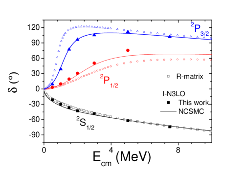
Figure 2: Low energy n-⁴He scattering phaseshifts calculated for the Hamiltonian based on I-N3LO nucleon-nucleon interaction. Results of this work (full symbols) are compared to ones obtained by NCSMC method Navrátil et al. (2016) (full lines). Theoretical calculations are also compared with the phaseshifts obtained from the R-matrix analysis of the experimental data Csótó and Hale (1997) (open symbols).

In Figure 2 $J^{\pi}=\frac{1}{2}^{\pm}$ and $J^{\pi}=\frac{3}{2}^{-}$ angular momenta phaseshifts calculated for I-N3LO Hamiltonian are compared with the results obtained using NCSMC technique Navrátil et al. (2016) as well as with phaseshifts extracted from experimental data performing R-matrix analysis Csótó and Hale (1997). Keeping in mind that both theoretical calculations – of this work as well as ones obtained using NCSMC technique Navrátil et al. (2016) – have comparable numerical accuracy of 1-2^∘ one may signal full agreement between two completely different approaches to solve elastic scattering problem. In that relates to comparison with the experimental data one may also signal nice agreement for the S-wave scattering, dominated by strong Pauli repulsion between projectile neutron and ones present within ⁴He target. On contrary description of resonant P-waves is not satisfactory, revealing insufficient splitting between $J^{\pi}=\frac{1}{2}^{-}$ and $J^{\pi}=\frac{3}{2}^{-}$ waves.

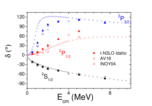
Figure 3: Comparison of low energy n-⁴He scattering phaseshifts calculated for different realistic NN interaction Hamiltonians: I-N3LO (full triangles), AV18 (crosses) and INOY04 (open squares). Theoretical calculations are also compared with the phaseshifts obtained from the R-matrix analysis of the experimental data Csótó and Hale (1997) (small open symbols).

In Figure 3 aforementioned I-N3LO Hamiltonian results are compared with those obtained for INOY04 and AV18 Hamiltonians. All the models describe well S-wave phaseshifts, indicating that description of these waves are model independent. On contrary different model predictions deviate in describing resonant scattering in P-waves. Both INOY04 and AV18 models lack attraction in $J^{\pi}=\frac{3}{2}^{-}$ wave, predicting much flatter resonant structure than provided by R-matrix analysis of the experimental data Csótó and Hale (1997) or even when compared to I-N3LO results. As a consequence splitting between two P-waves for AV18 model is smaller than for I-N3LO, which indicates necessity of weaker effective spin-orbit interaction for AV18 model than for I-N3LO. For INOY04 interaction simple splitting of P-waves is not enough to account for the experimental data, for this model P-wave needs to be much more attractive in overall. Worths noting that very similar observations has been made when studying neutron scattering on ³H nucleus Lazauskas and Carbonell (2004); Viviani et al. (2013, 2011): INOY04 model lacks strongly attraction in P-waves, AV18 also provides flatter than required resonant structures of ⁴H nucleus, whereas I-N3LO model provides the best description of the experimental data. This feature indicates on possible correlation between P-wave states of ⁵He and ⁴H (or its isospin symmetry partner ⁴Li nucleus).

It is well accepted that proper description of the nuclear systems requires presence of three-nucleon force. Modern models of three-nucleon forces provide an extra-binding for symmetric nuclei, like ground state of ⁴He, but also are able to invoke more attraction for P-wave states. It is demonstrated in Viviani et al. (2013) for n-³H scattering and in Navrátil et al. (2016) for n-⁴He case, that implementation of local 3NF force, developed up to N2LO terms in Navrátil (2007), in conjunction with I-N3LO interaction improves significantly description of P-wave resonant states. Very similar effects are observed when implementing phenomenological IL2 or IL7 three-nucleon forces Pieper et al. (2001); S.C. (2008) in conjunction with AV18 NN-interaction Viviani et al. (2013); Nollett et al. (2007). In this context case of INOY04 interaction turns to be quite nontrivial. On one hand this model provides proper binding energies of trinucleon(s), however it slightly overbinds ⁴He ground state by about 800 keV Lazauskas and Carbonell (2004). More importantly this model systematically underestimates mean square radii of the light nuclei Forssén et al. (2009) resulting large saturation densities of the symmetric nuclear matter Baldo and Maieron (2005). Finally, this model is unable to provide sufficiently attraction for P-wave structures. Therefore it should be highly nontrivial to correct all these defects by a simple model of 3NF. INOY04 would require 3NF, which is strongly repulsive at the origin in order to correct nuclear radii as well as saturation properties of the nuclear matter. On the other hand it would need some attraction in periphery with little effect on symmetric nuclei, whereas providing strong attraction for P-wave structures.

VI Conclusion

In the present paper the first solution of five-body Faddeev-Yakubovsky equations is presented, when describing neutron elastic scattering on ⁴He. The developed numerical method uses no uncontrolled approximations, is numerically very efficient and includes very large number of partial waves. These developments allows description of five-nucleon systems considering realistic nuclear Hamiltonians.

Three realistic nucleon-nucleon Hamiltonians have been tested, namely INOY04, I-N3LO and AV18. All of the considered models provide accurate description of low energy n-⁴He scattering in S-wave, dominated by strong Pauli repulsion. On contrary model predictions deviate from the phaseshifts derived from the experimental data for resonant P-wave scattering. Very similar effects have been observed when studying n-³H and p-³H scattering in Lazauskas and Carbonell (2004); Viviani et al. (2013, 2011), which indicates on the possible existence of strong correlations between four and five nucleon sector.

Acknowledgment. This work was granted access to the HPC resources of TGCC/IDRIS under the allocation 2016-x2016056006 made by GENCI (Grand Equipement National de Calcul Intensif).

References

- Pieper et al. (2002) S. Pieper, K. Varga, and R. Wiringa, PHYSICAL REVIEW C 66 (2002), ISSN 0556-2813.
- Hagen et al. (2010) G. Hagen, T. Papenbrock, D. J. Dean, and M. Hjorth-Jensen, PHYSICAL REVIEW C 82 (2010), ISSN 0556-2813.
- Barrett et al. (2013) B. R. Barrett, P. Navrátil, and J. P. Vary, Progress in Particle and Nuclear Physics 69, 131 (2013), ISSN 0146-6410, URL http://www.sciencedirect.com/science/article/pii/S0146641012001184.
- Tsukiyama et al. (2011) K. Tsukiyama, S. K. Bogner, and A. Schwenk, Phys. Rev. Lett. 106, 222502 (2011), URL https://link.aps.org/doi/10.1103/PhysRevLett.106.222502.
- Somà et al. (2013) V. Somà, C. Barbieri, and T. Duguet, Phys. Rev. C 87, 011303 (2013), URL https://link.aps.org/doi/10.1103/PhysRevC.87.011303.
- Faddeev (1961) L. D. Faddeev, Sov. Phys. JETP 12, 1014 (1961).
- Yakubovsky (1967) O. A. Yakubovsky, Sov. J. Nucl. Phys. 5, 937 (1967).
- Glöckle et al. (1996) W. Glöckle, H. Witala, D. Hüber, H. Kamada, and J. Golak, Physics Reports 274, 107 (1996), ISSN 0370-1573, URL http://www.sciencedirect.com/science/article/pii/0370157395000852.
- Viviani et al. (2017) M. Viviani, A. Deltuva, R. Lazauskas, A. C. Fonseca, A. Kievsky, and L. E. Marcucci, Phys. Rev. C 95, 034003 (2017), URL https://link.aps.org/doi/10.1103/PhysRevC.95.034003.
- Viviani et al. (1998) M. Viviani, S. Rosati, and A. Kievsky, Phys. Rev. Lett. 81, 1580 (1998).
- Navrátil et al. (2010) P. Navrátil, R. Roth, and S. Quaglioni, Phys. Rev. C 82, 034609 (2010), URL http://link.aps.org/doi/10.1103/PhysRevC.82.034609.
- Wiringa et al. (1995) R. B. Wiringa, V. G. J. Stoks, and R. Schiavilla, Phys. Rev. C 51, 38 (1995), URL https://link.aps.org/doi/10.1103/PhysRevC.51.38.
- Doleschall (2004) P. Doleschall, Phys. Rev. C 69, 054001 (2004), URL https://link.aps.org/doi/10.1103/PhysRevC.69.054001.
- Entem and Machleidt (2003) D. R. Entem and R. Machleidt, Phys. Rev. C 68, 041001 (2003), URL https://link.aps.org/doi/10.1103/PhysRevC.68.041001.
- Sasakawa (1977) T. Sasakawa, Progress of Theoretical Physics Supplement - PROG THEOR PHYS SUPPL 61, 149 (1977).
- Barletta et al. (2009) P. Barletta, C. Romero-Redondo, A. Kievsky, M. Viviani, and E. Garrido, Phys. Rev. Lett. 103, 090402 (2009), URL http://link.aps.org/doi/10.1103/PhysRevLett.103.090402.
- Kievsky et al. (2010a) A. Kievsky, M. Viviani, P. Barletta, C. Romero-Redondo, and E. Garrido, Phys. Rev. C 81, 034002 (2010a), URL http://link.aps.org/doi/10.1103/PhysRevC.81.034002.
- Baye (2015) D. Baye, Physics Reports 565, 1 (2015).
- Lazauskas (2003) R. Lazauskas, Ph.D. thesis, Université Joseph Fourier, Grenoble (2003), URL https://hal.archives-ouvertes.fr/tel-00004178.
- Lazauskas and Carbonell (2004) R. Lazauskas and J. Carbonell, Phys. Rev. C 70, 044002 (2004).
- Navrátil (2007) P. Navrátil, Few-Body Systems 41, 117 (2007), ISSN 1432-5411, URL https://doi.org/10.1007/s00601-007-0193-3.
- Deltuva and Fonseca (2007) A. Deltuva and A. C. Fonseca, Phys. Rev. C 75, 014005 (2007), URL https://link.aps.org/doi/10.1103/PhysRevC.75.014005.
- Kievsky et al. (2010b) A. Kievsky, M. Viviani, L. Girlanda, and L. E. Marcucci, Phys. Rev. C 81, 044003 (2010b), URL https://link.aps.org/doi/10.1103/PhysRevC.81.044003.
- Navrátil et al. (2016) P. Navrátil, S. Quaglioni, G. Hupin, C. Romero-Redondo, and A. Calci, Physica Scripta 91, 053002 (2016), URL http://stacks.iop.org/1402-4896/91/i=5/a=053002.
- Csótó and Hale (1997) A. Csótó and G. M. Hale, Phys. Rev. C 55, 536 (1997), URL https://link.aps.org/doi/10.1103/PhysRevC.55.536.
- Viviani et al. (2013) M. Viviani, L. Girlanda, A. Kievsky, and L. E. Marcucci, Phys. Rev. Lett. 111, 172302 (2013), URL https://link.aps.org/doi/10.1103/PhysRevLett.111.172302.
- Viviani et al. (2011) M. Viviani, A. Deltuva, R. Lazauskas, J. Carbonell, A. C. Fonseca, A. Kievsky, L. Marcucci, and S. Rosati, Phys. Rev. C 84, 054010 (2011), URL https://link.aps.org/doi/10.1103/PhysRevC.84.054010.
- Pieper et al. (2001) S. C. Pieper, V. R. Pandharipande, R. B. Wiringa, and J. Carlson, Phys. Rev. C 64, 014001 (2001), URL https://link.aps.org/doi/10.1103/PhysRevC.64.014001.
- S.C. (2008) P. S.C., AIP Conf. Proc. 1011, 143 (2008).
- Nollett et al. (2007) K. M. Nollett, S. C. Pieper, R. B. Wiringa, J. Carlson, and G. M. Hale, Phys. Rev. Lett. 99, 022502 (2007), URL https://link.aps.org/doi/10.1103/PhysRevLett.99.022502.
- Forssén et al. (2009) C. Forssén, E. Caurier, and P. Navrátil, Phys. Rev. C 79, 021303 (2009), URL https://link.aps.org/doi/10.1103/PhysRevC.79.021303.
- Baldo and Maieron (2005) M. Baldo and C. Maieron, Phys. Rev. C 72, 034005 (2005), URL https://link.aps.org/doi/10.1103/PhysRevC.72.034005.